OPEN-SOURCE SCRIPT
Ehlers Even Better Sinewave (EBSW)
# EBSW: Ehlers Even Better Sinewave
## Overview and Purpose
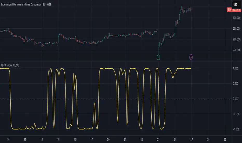
The Ehlers Even Better Sinewave (EBSW) indicator, developed by John Ehlers, is an advanced cycle analysis tool. This implementation is based on a common interpretation that uses a cascade of filters: first, a High-Pass Filter (HPF) to detrend price data, followed by a Super Smoother Filter (SSF) to isolate the dominant cycle. The resulting filtered wave is then normalized using an Automatic Gain Control (AGC) mechanism, producing a bounded oscillator that fluctuates between approximately +1 and -1. It aims to provide a clear and responsive measure of market cycles.
## Core Concepts
* **Detrending (High-Pass Filter):** A 1-pole High-Pass Filter removes the longer-term trend component from the price data, allowing the indicator to focus on cyclical movements.
* **Cycle Smoothing (Super Smoother Filter):** Ehlers' Super Smoother Filter is applied to the detrended data to further refine the cycle component, offering effective smoothing with relatively low lag.
* **Wave Generation:** The output of the SSF is averaged over a short period (typically 3 bars) to create the primary "wave".
* **Automatic Gain Control (AGC):** The wave's amplitude is normalized by dividing it by the square root of its recent power (average of squared values). This keeps the oscillator bounded and responsive to changes in volatility.
* **Normalized Oscillator:** The final output is a single sinewave-like oscillator.
## Common Settings and Parameters
| Parameter | Default | Function | When to Adjust |
| ----------- | ------- | --------------------------------------------------------------------------------------------- | ----------------------------------------------------------------------------------------------------------------------------------------------- |
| Source | close | Price data used for calculation. | Typically `close`, but `hlc3` or `ohlc4` can be used for a more comprehensive price representation. |
| HP Length | 40 | Lookback period for the 1-pole High-Pass Filter used for detrending. | Shorter periods make the filter more responsive to shorter cycles; longer periods focus on longer-term cycles. Adjust based on observed cycle characteristics. |
| SSF Length | 10 | Lookback period for the Super Smoother Filter used for smoothing the detrended cycle component. | Shorter periods result in a more responsive (but potentially noisier) wave; longer periods provide more smoothing. |
**Pro Tip:** The `HP Length` and `SSF Length` parameters should be tuned based on the typical cycle lengths observed in the market and the desired responsiveness of the indicator.
## Calculation and Mathematical Foundation
**Simplified explanation:**
1. Remove the trend from the price data using a 1-pole High-Pass Filter.
2. Smooth the detrended data using a Super Smoother Filter to get a clean cycle component.
3. Average the output of the Super Smoother Filter over the last 3 bars to create a "Wave".
4. Calculate the average "Power" of the Super Smoother Filter output over the last 3 bars.
5. Normalize the "Wave" by dividing it by the square root of the "Power" to get the final EBSW value.
**Technical formula (conceptual):**
1. **High-Pass Filter (HPF - 1-pole):**
`angle_hp = 2 * PI / hpLength`
`alpha1_hp = (1 - sin(angle_hp)) / cos(angle_hp)`
`HP = (0.5 * (1 + alpha1_hp) * (src - src[1])) + alpha1_hp * HP[1]`
2. **Super Smoother Filter (SSF):**
`angle_ssf = sqrt(2) * PI / ssfLength`
`alpha2_ssf = exp(-angle_ssf)`
`beta_ssf = 2 * alpha2_ssf * cos(angle_ssf)`
`c2 = beta_ssf`
`c3 = -alpha2_ssf^2`
`c1 = 1 - c2 - c3`
`Filt = c1 * (HP + HP[1])/2 + c2*Filt[1] + c3*Filt[2]`
3. **Wave Generation:**
`WaveVal = (Filt + Filt[1] + Filt[2]) / 3`
4. **Power & Automatic Gain Control (AGC):**
`Pwr = (Filt^2 + Filt[1]^2 + Filt[2]^2) / 3`
`EBSW_SineWave = WaveVal / sqrt(Pwr)` (with check for Pwr == 0)
> 🔍 **Technical Note:** The combination of HPF and SSF creates a form of band-pass filter. The AGC mechanism ensures the output remains scaled, typically between -1 and +1, making it behave like a normalized oscillator.
## Interpretation Details
* **Cycle Identification:** The EBSW wave shows the current phase and strength of the dominant market cycle as filtered by the indicator. Peaks suggest cycle tops, and troughs suggest cycle bottoms.
* **Trend Reversals/Momentum Shifts:** When the EBSW wave crosses the zero line, it can indicate a potential shift in the short-term cyclical momentum.
* Crossing up through zero: Potential start of a bullish cyclical phase.
* Crossing down through zero: Potential start of a bearish cyclical phase.
* **Overbought/Oversold Levels:** While normalized, traders often establish subjective or statistically derived overbought/oversold levels (e.g., +0.85 and -0.85, or other values like +0.7, +0.9).
* Reaching above the overbought level and turning down may signal a potential cyclical peak.
* Falling below the oversold level and turning up may signal a potential cyclical trough.
## Limitations and Considerations
* **Parameter Sensitivity:** The indicator's performance depends on tuning `hpLength` and `ssfLength` to prevailing market conditions.
* **Non-Stationary Markets:** In strongly trending markets with weak cyclical components, or in very choppy non-cyclical conditions, the EBSW may produce less reliable signals.
* **Lag:** All filtering introduces some lag. The Super Smoother Filter is designed to minimize this for its degree of smoothing, but lag is still present.
* **Whipsaws:** Rapid oscillations around the zero line can occur in volatile or directionless markets.
* **Requires Confirmation:** Signals from EBSW are often best confirmed with other forms of technical analysis (e.g., price action, volume, other non-correlated indicators).
## References
* Ehlers, J. F. (2002). *Rocket Science for Traders: Digital Signal Processing Applications*. John Wiley & Sons.
* Ehlers, J. F. (2013). *Cycle Analytics for Traders: Advanced Technical Trading Concepts*. John Wiley & Sons.
## Overview and Purpose
The Ehlers Even Better Sinewave (EBSW) indicator, developed by John Ehlers, is an advanced cycle analysis tool. This implementation is based on a common interpretation that uses a cascade of filters: first, a High-Pass Filter (HPF) to detrend price data, followed by a Super Smoother Filter (SSF) to isolate the dominant cycle. The resulting filtered wave is then normalized using an Automatic Gain Control (AGC) mechanism, producing a bounded oscillator that fluctuates between approximately +1 and -1. It aims to provide a clear and responsive measure of market cycles.
## Core Concepts
* **Detrending (High-Pass Filter):** A 1-pole High-Pass Filter removes the longer-term trend component from the price data, allowing the indicator to focus on cyclical movements.
* **Cycle Smoothing (Super Smoother Filter):** Ehlers' Super Smoother Filter is applied to the detrended data to further refine the cycle component, offering effective smoothing with relatively low lag.
* **Wave Generation:** The output of the SSF is averaged over a short period (typically 3 bars) to create the primary "wave".
* **Automatic Gain Control (AGC):** The wave's amplitude is normalized by dividing it by the square root of its recent power (average of squared values). This keeps the oscillator bounded and responsive to changes in volatility.
* **Normalized Oscillator:** The final output is a single sinewave-like oscillator.
## Common Settings and Parameters
| Parameter | Default | Function | When to Adjust |
| ----------- | ------- | --------------------------------------------------------------------------------------------- | ----------------------------------------------------------------------------------------------------------------------------------------------- |
| Source | close | Price data used for calculation. | Typically `close`, but `hlc3` or `ohlc4` can be used for a more comprehensive price representation. |
| HP Length | 40 | Lookback period for the 1-pole High-Pass Filter used for detrending. | Shorter periods make the filter more responsive to shorter cycles; longer periods focus on longer-term cycles. Adjust based on observed cycle characteristics. |
| SSF Length | 10 | Lookback period for the Super Smoother Filter used for smoothing the detrended cycle component. | Shorter periods result in a more responsive (but potentially noisier) wave; longer periods provide more smoothing. |
**Pro Tip:** The `HP Length` and `SSF Length` parameters should be tuned based on the typical cycle lengths observed in the market and the desired responsiveness of the indicator.
## Calculation and Mathematical Foundation
**Simplified explanation:**
1. Remove the trend from the price data using a 1-pole High-Pass Filter.
2. Smooth the detrended data using a Super Smoother Filter to get a clean cycle component.
3. Average the output of the Super Smoother Filter over the last 3 bars to create a "Wave".
4. Calculate the average "Power" of the Super Smoother Filter output over the last 3 bars.
5. Normalize the "Wave" by dividing it by the square root of the "Power" to get the final EBSW value.
**Technical formula (conceptual):**
1. **High-Pass Filter (HPF - 1-pole):**
`angle_hp = 2 * PI / hpLength`
`alpha1_hp = (1 - sin(angle_hp)) / cos(angle_hp)`
`HP = (0.5 * (1 + alpha1_hp) * (src - src[1])) + alpha1_hp * HP[1]`
2. **Super Smoother Filter (SSF):**
`angle_ssf = sqrt(2) * PI / ssfLength`
`alpha2_ssf = exp(-angle_ssf)`
`beta_ssf = 2 * alpha2_ssf * cos(angle_ssf)`
`c2 = beta_ssf`
`c3 = -alpha2_ssf^2`
`c1 = 1 - c2 - c3`
`Filt = c1 * (HP + HP[1])/2 + c2*Filt[1] + c3*Filt[2]`
3. **Wave Generation:**
`WaveVal = (Filt + Filt[1] + Filt[2]) / 3`
4. **Power & Automatic Gain Control (AGC):**
`Pwr = (Filt^2 + Filt[1]^2 + Filt[2]^2) / 3`
`EBSW_SineWave = WaveVal / sqrt(Pwr)` (with check for Pwr == 0)
> 🔍 **Technical Note:** The combination of HPF and SSF creates a form of band-pass filter. The AGC mechanism ensures the output remains scaled, typically between -1 and +1, making it behave like a normalized oscillator.
## Interpretation Details
* **Cycle Identification:** The EBSW wave shows the current phase and strength of the dominant market cycle as filtered by the indicator. Peaks suggest cycle tops, and troughs suggest cycle bottoms.
* **Trend Reversals/Momentum Shifts:** When the EBSW wave crosses the zero line, it can indicate a potential shift in the short-term cyclical momentum.
* Crossing up through zero: Potential start of a bullish cyclical phase.
* Crossing down through zero: Potential start of a bearish cyclical phase.
* **Overbought/Oversold Levels:** While normalized, traders often establish subjective or statistically derived overbought/oversold levels (e.g., +0.85 and -0.85, or other values like +0.7, +0.9).
* Reaching above the overbought level and turning down may signal a potential cyclical peak.
* Falling below the oversold level and turning up may signal a potential cyclical trough.
## Limitations and Considerations
* **Parameter Sensitivity:** The indicator's performance depends on tuning `hpLength` and `ssfLength` to prevailing market conditions.
* **Non-Stationary Markets:** In strongly trending markets with weak cyclical components, or in very choppy non-cyclical conditions, the EBSW may produce less reliable signals.
* **Lag:** All filtering introduces some lag. The Super Smoother Filter is designed to minimize this for its degree of smoothing, but lag is still present.
* **Whipsaws:** Rapid oscillations around the zero line can occur in volatile or directionless markets.
* **Requires Confirmation:** Signals from EBSW are often best confirmed with other forms of technical analysis (e.g., price action, volume, other non-correlated indicators).
## References
* Ehlers, J. F. (2002). *Rocket Science for Traders: Digital Signal Processing Applications*. John Wiley & Sons.
* Ehlers, J. F. (2013). *Cycle Analytics for Traders: Advanced Technical Trading Concepts*. John Wiley & Sons.
Skrip sumber terbuka
Dalam semangat TradingView sebenar, pencipta skrip ini telah menjadikannya sumber terbuka, jadi pedagang boleh menilai dan mengesahkan kefungsiannya. Terima kasih kepada penulis! Walaupuan anda boleh menggunakan secara percuma, ingat bahawa penerbitan semula kod ini tertakluk kepada Peraturan Dalaman.
github.com/mihakralj/pinescript
A collection of mathematically rigorous technical indicators for Pine Script 6, featuring defensible math, optimized implementations, proper state initialization, and O(1) constant time efficiency where possible.
A collection of mathematically rigorous technical indicators for Pine Script 6, featuring defensible math, optimized implementations, proper state initialization, and O(1) constant time efficiency where possible.
Penafian
Maklumat dan penerbitan adalah tidak bertujuan, dan tidak membentuk, nasihat atau cadangan kewangan, pelaburan, dagangan atau jenis lain yang diberikan atau disahkan oleh TradingView. Baca lebih dalam Terma Penggunaan.