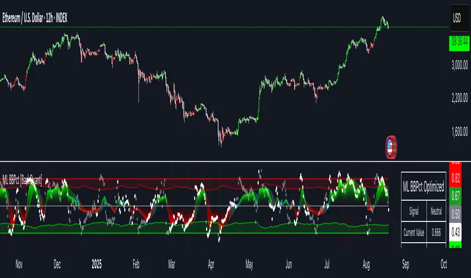
Machine Learning BBPct [BackQuant]Machine Learning BBPct
What this is (in one line)
A Bollinger Band %B oscillator enhanced with a simplified K-Nearest Neighbors (KNN) pattern matcher. The model compares today’s context (volatility, momentum, volume, and position inside the bands) to similar situations in recent history and blends that historical consensus back into the raw %B to reduce noise and improve context awareness. It is informational and diagnostic—designed to describe market state, not to sell a trading system.
Background: %B in plain terms
Bollinger %B measures where price sits inside its dynamic envelope: 0 at the lower band, 1 at the upper band, ~ 0.5 near the basis (the moving average). Readings toward 1 indicate pressure near the envelope’s upper edge (often strength or stretch), while readings toward 0 indicate pressure near the lower edge (often weakness or stretch). Because bands adapt to volatility, %B is naturally comparable across regimes.
Why add (simplified) KNN?
Classic %B is reactive and can be whippy in fast regimes. The simplified KNN layer builds a “nearest-neighbor memory” of recent market states and asks: “When the market looked like this before, where did %B tend to be next bar?” It then blends that estimate with the current %B. Key ideas:
• Feature vector . Each bar is summarized by up to five normalized features:
– %B itself (normalized)
– Band width (volatility proxy)
– Price momentum (ROC)
– Volume momentum (ROC of volume)
– Price position within the bands
• Distance metric . Euclidean distance ranks the most similar recent bars.
• Prediction . Average the neighbors’ prior %B (lagged to avoid lookahead), inverse-weighted by distance.
• Blend . Linearly combine raw %B and KNN-predicted %B with a configurable weight; optional filtering then adapts to confidence.
This remains “simplified” KNN: no training/validation split, no KD-trees, no scaling beyond windowed min-max, and no probabilistic calibration.
How the script is organized (by input groups)
1) BBPct Settings
• Price Source – Which price to evaluate (%B is computed from this).
• Calculation Period – Lookback for SMA basis and standard deviation.
• Multiplier – Standard deviation width (e.g., 2.0).
• Apply Smoothing / Type / Length – Optional smoothing of the %B stream before ML (EMA, RMA, DEMA, TEMA, LINREG, HMA, etc.). Turning this off gives you the raw %B.
2) Thresholds
• Overbought/Oversold – Default 0.8 / 0.2 (inside ).
• Extreme OB/OS – Stricter zones (e.g., 0.95 / 0.05) to flag stretch conditions.
3) KNN Machine Learning
• Enable KNN – Switch between pure %B and hybrid.
• K (neighbors) – How many historical analogs to blend (default 8).
• Historical Period – Size of the search window for neighbors.
• ML Weight – Blend between raw %B and KNN estimate.
• Number of Features – Use 2–5 features; higher counts add context but raise the risk of overfitting in short windows.
4) Filtering
• Method – None, Adaptive, Kalman-style (first-order),
or Hull smoothing.
• Strength – How aggressively to smooth. “Adaptive” uses model confidence to modulate its alpha: higher confidence → stronger reliance on the ML estimate.
5) Performance Tracking
• Win-rate Period – Simple running score of past signal outcomes based on target/stop/time-out logic (informational, not a robust backtest).
• Early Entry Lookback – Horizon for forecasting a potential threshold cross.
• Profit Target / Stop Loss – Used only by the internal win-rate heuristic.
6) Self-Optimization
• Enable Self-Optimization – Lightweight, rolling comparison of a few canned settings (K = 8/14/21 via simple rules on %B extremes).
• Optimization Window & Stability Threshold – Governs how quickly preferred K changes and how sensitive the overfitting alarm is.
• Adaptive Thresholds – Adjust the OB/OS lines with volatility regime (ATR ratio), widening in calm markets and tightening in turbulent ones (bounded 0.7–0.9 and 0.1–0.3).
7) UI Settings
• Show Table / Zones / ML Prediction / Early Signals – Toggle informational overlays.
• Signal Line Width, Candle Painting, Colors – Visual preferences.
Step-by-step logic
A) Compute %B
Basis = SMA(source, len); dev = stdev(source, len) × multiplier; Upper/Lower = Basis ± dev.
%B = (price − Lower) / (Upper − Lower). Optional smoothing yields standardBB .
B) Build the feature vector
All features are min-max normalized over the KNN window so distances are in comparable units. Features include normalized %B, normalized band width, normalized price ROC, normalized volume ROC, and normalized position within bands. You can limit to the first N features (2–5).
C) Find nearest neighbors
For each bar inside the lookback window, compute the Euclidean distance between current features and that bar’s features. Sort by distance, keep the top K .
D) Predict and blend
Use inverse-distance weights (with a strong cap for near-zero distances) to average neighbors’ prior %B (lagged by one bar). This becomes the KNN estimate. Blend it with raw %B via the ML weight. A variance of neighbor %B around the prediction becomes an uncertainty proxy ; combined with a stability score (how long parameters remain unchanged), it forms mlConfidence ∈ . The Adaptive filter optionally transforms that confidence into a smoothing coefficient.
E) Adaptive thresholds
Volatility regime (ATR(14) divided by its 50-bar SMA) nudges OB/OS thresholds wider or narrower within fixed bounds. The aim: comparable extremeness across regimes.
F) Early entry heuristic
A tiny two-step slope/acceleration probe extrapolates finalBB forward a few bars. If it is on track to cross OB/OS soon (and slope/acceleration agree), it flags an EARLY_BUY/SELL candidate with an internal confidence score. This is explicitly a heuristic—use as an attention cue, not a signal by itself.
G) Informational win-rate
The script keeps a rolling array of trade outcomes derived from signal transitions + rudimentary exits (target/stop/time). The percentage shown is a rough diagnostic , not a validated backtest.
Outputs and visual language
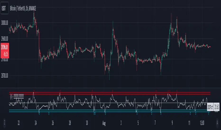
• ML Bollinger %B (finalBB) – The main line after KNN blending and optional filtering.
• Gradient fill – Greenish tones above 0.5, reddish below, with intensity following distance from the midline.
• Adaptive zones – Overbought/oversold and extreme bands; shaded backgrounds appear at extremes.
• ML Prediction (dots) – The KNN estimate plotted as faint circles; becomes bright white when confidence > 0.7.
• Early arrows – Optional small triangles for approaching OB/OS.
• Candle painting – Light green above the midline, light red below (optional).
• Info panel – Current value, signal classification, ML confidence, optimized K, stability, volatility regime, adaptive thresholds, overfitting flag, early-entry status, and total signals processed.
Signal classification (informational)
The indicator does not fire trade commands; it labels state:
• STRONG_BUY / STRONG_SELL – finalBB beyond extreme OS/OB thresholds.
• BUY / SELL – finalBB beyond adaptive OS/OB.
• EARLY_BUY / EARLY_SELL – forecast suggests a near-term cross with decent internal confidence.
• NEUTRAL – between adaptive bands.
Alerts (what you can automate)
• Entering adaptive OB/OS and extreme OB/OS.
• Midline cross (0.5).
• Overfitting detected (frequent parameter flipping).
• Early signals when early confidence > 0.7.
These are purely descriptive triggers around the indicator’s state.
Practical interpretation
• Mean-reversion context – In range markets, adaptive OS/OB with ML smoothing can reduce whipsaws relative to raw %B.
• Trend context – In persistent trends, the KNN blend can keep finalBB nearer the mid/upper region during healthy pullbacks if history supports similar contexts.
• Regime awareness – Watch the volatility regime and adaptive thresholds. If thresholds compress (high vol), “OB/OS” comes sooner; if thresholds widen (calm), it takes more stretch to flag.
• Confidence as a weight – High mlConfidence implies neighbors agree; you may rely more on the ML curve. Low confidence argues for de-emphasizing ML and leaning on raw %B or other tools.
• Stability score – Rising stability indicates consistent parameter selection and fewer flips; dropping stability hints at a shifting backdrop.
Methodological notes
• Normalization uses rolling min-max over the KNN window. This is simple and scale-agnostic but sensitive to outliers; the distance metric will reflect that.
• Distance is unweighted Euclidean. If you raise featureCount, you increase dimensionality; consider keeping K larger and lookback ample to avoid sparse-neighbor artifacts.
• Lag handling intentionally uses neighbors’ previous %B for prediction to avoid lookahead bias.
• Self-optimization is deliberately modest: it only compares a few canned K/threshold choices using simple “did an extreme anticipate movement?” scoring, then enforces a stability regime and an overfitting guard. It is not a grid search or GA.
• Kalman option is a first-order recursive filter (fixed gain), not a full state-space estimator.
• Hull option derives a dynamic length from 1/strength; it is a convenience smoothing alternative.
Limitations and cautions
• Non-stationarity – Nearest neighbors from the recent window may not represent the future under structural breaks (policy shifts, liquidity shocks).
• Curse of dimensionality – Adding features without sufficient lookback can make genuine neighbors rare.
• Overfitting risk – The script includes a crude overfitting detector (frequent parameter flips) and will fall back to defaults when triggered, but this is only a guardrail.
• Win-rate display – The internal score is illustrative; it does not constitute a tradable backtest.
• Latency vs. smoothness – Smoothing and ML blending reduce noise but add lag; tune to your timeframe and objectives.
Tuning guide
• Short-term scalping – Lower len (10–14), slightly lower multiplier (1.8–2.0), small K (5–8), featureCount 3–4, Adaptive filter ON, moderate strength.
• Swing trading – len (20–30), multiplier ~2.0, K (8–14), featureCount 4–5, Adaptive thresholds ON, filter modest.
• Strong trends – Consider higher adaptive_upper/lower bounds (or let volatility regime do it), keep ML weight moderate so raw %B still reflects surges.
• Chop – Higher ML weight and stronger Adaptive filtering; accept lag in exchange for fewer false extremes.
How to use it responsibly
Treat this as a state descriptor and context filter. Pair it with your execution signals (structure breaks, volume footprints, higher-timeframe bias) and risk management. If mlConfidence is low or stability is falling, lean less on the ML line and more on raw %B or external confirmation.
Summary
Machine Learning BBPct augments a familiar oscillator with a transparent, simplified KNN memory of recent conditions. By blending neighbors’ behavior into %B and adapting thresholds to volatility regime—while exposing confidence, stability, and a plain early-entry heuristic—it provides an informational, probability-minded view of stretch and reversion that you can interpret alongside your own process.
Penunjuk Pine Script®