PatternTransitionTablesPatternTransitionTables Library
🌸 Part of GoemonYae Trading System (GYTS) 🌸
🌸 --------- 1. INTRODUCTION --------- 🌸
💮 Overview
This library provides precomputed state transition tables to enable ultra-efficient, O(1) computation of Ordinal Patterns. It is designed specifically to support high-performance indicators calculating Permutation Entropy and related complexity measures.
💮 The Problem & Solution
Calculating Permutation Entropy, as introduced by Bandt and Pompe (2002), typically requires computing ordinal patterns within a sliding window at every time step. The standard successive-pattern method (Equations 2+3 in the paper) requires ≤ 4d-1 operations per update.
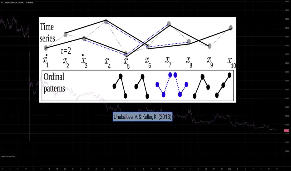
Unakafova and Keller (2013) demonstrated that successive ordinal patterns "overlap" significantly. By knowing the current pattern index and the relative rank (position l) of just the single new data point, the next pattern index can be determined via a precomputed look-up table. Computing l still requires d comparisons, but the table lookup itself is O(1), eliminating the need for d multiplications and d additions. This reduces total operations from ≤ 4d-1 to ≤ 2d per update (Table 4). This library contains these precomputed tables for orders d = 2 through d = 5.
🌸 --------- 2. THEORETICAL BACKGROUND --------- 🌸
💮 Permutation Entropy
Bandt, C., & Pompe, B. (2002). Permutation entropy: A natural complexity measure for time series.
doi.org
This concept quantifies the complexity of a system by comparing the order of neighbouring values rather than their magnitudes. It is robust against noise and non-linear distortions, making it ideal for financial time series analysis.
💮 Efficient Computation
Unakafova, V. A., & Keller, K. (2013). Efficiently Measuring Complexity on the Basis of Real-World Data.
doi.org
This library implements the transition function φ_d(n, l) described in Equation 5 of the paper. It maps a current pattern index (n) and the position of the new value (l) to the successor pattern, reducing the complexity of updates to constant time O(1).
🌸 --------- 3. LIBRARY FUNCTIONALITY --------- 🌸
💮 Data Structure
The library stores transition matrices as flattened 1D integer arrays. These tables are mathematically rigorous representations of the factorial number system used to enumerate permutations.
💮 Core Function: get_successor()
This is the primary interface for the library for direct pattern updates.
• Input: The current pattern index and the rank position of the incoming price data.
• Process: Routes the request to the specific transition table for the chosen order (d=2 to d=5).
• Output: The integer index of the next ordinal pattern.
💮 Table Access: get_table()
This function returns the entire flattened transition table for a specified dimension. This enables local caching of the table (e.g. in an indicator's init() method), avoiding the overhead of repeated library calls during the calculation loop.
💮 Supported Orders & Terminology
The parameter d is the order of ordinal patterns (following Bandt & Pompe 2002). Each pattern of order d contains (d+1) data points, yielding (d+1)! unique patterns:
• d=2: 3 points → 6 unique patterns, 3 successor positions
• d=3: 4 points → 24 unique patterns, 4 successor positions
• d=4: 5 points → 120 unique patterns, 5 successor positions
• d=5: 6 points → 720 unique patterns, 6 successor positions
Note: d=6 is not implemented. The resulting code size (approx. 191k tokens) exceeds the Pine Script limit of 100k tokens (as of 2025-12).
Chaostheory
Fractal Fade Pro IndicatorA revolutionary contrarian trading indicator that applies chaos theory, fractal mathematics, and market entropy to generate high-probability reverse signals. This indicator fades traditional technical signals, providing BUY signals when conventional indicators say SELL, and SELL signals when they say BUY.
Full Description:
Most traders follow the herd. QFCI does the opposite. It identifies when conventional technical analysis is about to fail by detecting mathematical patterns of exhaustion in market structure.
How It Works (Technical Overview):
The indicator combines three sophisticated mathematical approaches:
Fractal Dimension Analysis: Measures the "roughness" of price movements using fractal mathematics
Market Entropy Calculation: Quantifies the randomness and disorder in price returns using information theory
Phase Space Reconstruction: Analyzes price evolution in multi-dimensional state space from chaos theory
Signal Generation Process:
Step 1: Market Regime Detection
Chaotic Regime: High fractal complexity + rising entropy (avoid trading)
Trending Regime: Low fractal complexity + high phase space distance (fade breakouts)
Mean-Reverting Regime: Very low fractal complexity (fade extremes)
Step 2: Reverse Signal Logic
When traditional indicators would give:
BUY signal (breakout, oversold bounce, volatility spike) → QFCI shows SELL
SELL signal (breakdown, overbought rejection, volatility crash) → QFCI shows BUY
Step 3: Smart Signal Filtering
No consecutive same-direction signals
Adjustable minimum bars between signals
Multiple confirmation layers required
Unique Features:
1. Mathematical Innovation:
Original fractal dimension algorithm (not standard indicators)
Market entropy calculation from information theory
Phase space reconstruction from chaos theory
Multi-regime adaptive logic
2. Trading Psychology Advantage:
Contrarian by design - profits from market overreactions
Fades retail trader mistakes - enters when others are exiting
Reduces overtrading - strict signal frequency controls
3. Clean Visual Interface:
Only BUY/SELL labels - no chart clutter
Clear directional arrows - immediate signal recognition
Built-in alerts - never miss a trade
Recommended Settings:
Default (Balanced Approach):
Fractal Depth: 20
Entropy Period: 200
Min Bars Between Signals: 100
Aggressive Trading:
Fractal Depth: 10-15
Entropy Period: 100-150
Min Bars Between Signals: 50-75
Conservative Trading:
Fractal Depth: 30-40
Entropy Period: 300-400
Min Bars Between Signals: 150-200
Optimal Timeframes:
Primary: Daily, Weekly (best performance)
Secondary: 4-Hour, 12-Hour
Can work on: 1-Hour (with adjusted parameters)
How to Use:
For Beginners:
Apply indicator to chart
Use default settings
Wait for BUY/SELL labels
Enter on next candle open
Use 2:1 risk/reward ratio
Always use stop losses
For Advanced Traders:
Adjust parameters for your trading style
Combine with support/resistance levels
Use volume confirmation
Scale in/out of positions
Track performance by regime
Risk Management Guidelines:
Position Sizing:
Conservative: 1-2% risk per trade
Moderate: 2-3% risk per trade
Aggressive: 3-5% risk per trade (not recommended)
Stop Loss Placement:
BUY signals: Below recent swing low or -2x ATR
SELL signals: Above recent swing high or +2x ATR
Take Profit Targets:
Primary: 2x risk (minimum)
Secondary: Previous support/resistance
Tertiary: Trailing stops after 1.5x risk
IMPORTANT RISK DISCLOSURE
This indicator is for educational and informational purposes only. It is not financial advice. Past performance does not guarantee future results. Trading involves substantial risk of loss and is not suitable for every investor. The risk of loss in trading can be substantial. You should therefore carefully consider whether such trading is suitable for you in light of your financial condition.

Bifurcation Early WarningBifurcation Early Warning (BEW) — Chaos Theory Regime Detection
OVERVIEW
The Bifurcation Early Warning indicator applies principles from chaos theory and complex systems research to detect when markets are approaching critical transition points — moments where the current regime is likely to break down and shift to a new state.
Unlike momentum or trend indicators that tell you what is happening, BEW tells you when something is about to change. It provides early warning of regime shifts before they occur, giving traders time to prepare for increased volatility or trend reversals.
THE SCIENCE BEHIND IT
In complex systems (weather, ecosystems, financial markets), major transitions don't happen randomly. Research has identified three universal warning signals that precede critical transitions:
1. Critical Slowing Down
As a system approaches a tipping point, it becomes "sluggish" — small perturbations take longer to decay. In markets, this manifests as rising autocorrelation in returns.
2. Variance Amplification
Short-term volatility begins expanding relative to longer-term baselines as the system destabilizes.
3. Flickering
The system oscillates between two potential states before committing to one — visible as increased crossing of mean levels.
BEW combines all three signals into a single composite score.
COMPONENTS
AR(1) Coefficient — Critical Slowing Down (Blue)
Measures lag-1 autocorrelation of returns over a rolling window.
• Rising toward 1.0: Market becoming "sticky," slow to mean-revert — transition approaching
• Low values (<0.3): Normal mean-reverting behavior, stable regime
Variance Ratio (Purple)
Compares short-term variance to long-term variance.
• Above 1.5: Short-term volatility expanding — energy building before a move
• Near 1.0: Volatility stable, no unusual pressure
Flicker Count (Yellow/Teal)
Counts state changes (crossings of the dynamic mean) within the lookback period.
• High count: Market oscillating between states — indecision before commitment
• Low count: Price firmly in one regime
INTERPRETING THE BEW SCORE
0–50 (STABLE): Normal market conditions. Existing strategies should perform as expected.
50–70 (WARNING): Elevated instability detected. Consider reducing exposure or tightening risk parameters.
70–85 (DANGER): High probability of regime change. Avoid initiating new positions; widen stops on existing ones.
85+ (CRITICAL): Bifurcation likely imminent or in progress. Expect large, potentially unpredictable moves.
HOW TO USE
As a Regime Filter
• BEW < 50: Normal trading conditions — apply your standard strategies
• BEW > 60: Elevated caution — reduce position sizes, avoid mean-reversion plays
• BEW > 80: High alert — consider staying flat or hedging existing positions
As a Preparation Signal
BEW tells you when to pay attention, not which direction. When readings elevate:
• Watch for confirmation from volume, order flow, or other directional indicators
• Prepare for breakout scenarios in either direction
• Adjust take-profit and stop-loss distances for larger moves
For Volatility Adjustment
High BEW periods correlate with larger candles. Use this to:
• Widen stops during elevated readings
• Adjust position sizing inversely to BEW score
• Set more ambitious profit targets when entering during high-BEW breakouts
Divergence Analysis
• Price making new highs/lows while BEW stays low: Trend likely to continue smoothly
• Price consolidating while BEW rises: Breakout incoming — direction uncertain but move will be significant
SETTINGS GUIDE
Core Settings
• Lookback Period: General reference period (default: 50)
• Source: Price source for calculations (default: close)
Critical Slowing Down (AR1)
• AR(1) Calculation Period: Bars used for autocorrelation (default: 100). Higher = smoother, slower.
• AR(1) Warning Threshold: Level at which AR(1) is considered elevated (default: 0.85)
Variance Growth
• Variance Short Period: Fast variance window (default: 20)
• Variance Long Period: Slow variance window (default: 100)
• Variance Ratio Threshold: Level for maximum score contribution (default: 1.5)
Regime Flickering
• Flicker Detection Period: Window for counting state changes (default: 20)
• Flicker Bandwidth: ATR multiplier for state detection — lower = more sensitive (default: 0.5)
• Flicker Count Threshold: Number of crossings for maximum score (default: 4)
TIMEFRAME RECOMMENDATIONS
• 5m–15m: Use shorter periods (AR: 30–50, Var: 10/50). Expect more noise.
• 1H: Balanced performance with default or slightly extended settings (AR: 100, Var: 20/100).
• 4H–Daily: Extend periods further (AR: 100–150, Var: 30/150). Cleaner signals, less frequent.
ALERTS
Three alert conditions are included:
• BEW Warning: Score crosses above 50
• BEW Danger: Score crosses above 70
• BEW Critical: Score crosses above 85
LIMITATIONS
• No directional bias: BEW detects instability, not direction. Combine with trend or momentum indicators.
• Not a timing tool: Elevated readings may persist for several bars before the actual move.
• Parameter sensitive: Optimal settings vary by asset and timeframe. Backtest before live use.
• Leading indicator trade-off: Early warning means some false positives are inevitable.
CREDITS
Inspired by research on early warning signals in complex systems:
• Dakos et al. (2012) — "Methods for detecting early warnings of critical transitions"
DISCLAIMER
This indicator is for educational and informational purposes only. It does not constitute financial advice. Past performance is not indicative of future results. Always conduct your own analysis and risk management. Use at your own risk.

Lyapunov Hodrick-Prescott Oscillator w/ DSL [Loxx]Lyapunov Hodrick-Prescott Oscillator w/ DSL is a Hodrick-Prescott Channel Filter that is modified using the Lyapunov stability algorithm to turn the filter into an oscillator. Signals are created using Discontinued Signal Lines.
What is the Lyapunov Stability?
As soon as scientists realized that the evolution of physical systems can be described in terms of mathematical equations, the stability of the various dynamical regimes was recognized as a matter of primary importance. The interest for this question was not only motivated by general curiosity, but also by the need to know, in the XIX century, to what extent the behavior of suitable mechanical devices remains unchanged, once their configuration has been perturbed. As a result, illustrious scientists such as Lagrange, Poisson, Maxwell and others deeply thought about ways of quantifying the stability both in general and specific contexts. The first exact definition of stability was given by the Russian mathematician Aleksandr Lyapunov who addressed the problem in his PhD Thesis in 1892, where he introduced two methods, the first of which is based on the linearization of the equations of motion and has originated what has later been termed Lyapunov exponents (LE). (Lyapunov 1992)
The interest in it suddenly skyrocketed during the Cold War period when the so-called "Second Method of Lyapunov" (see below) was found to be applicable to the stability of aerospace guidance systems which typically contain strong nonlinearities not treatable by other methods. A large number of publications appeared then and since in the control and systems literature. More recently the concept of the Lyapunov exponent (related to Lyapunov's First Method of discussing stability) has received wide interest in connection with chaos theory . Lyapunov stability methods have also been applied to finding equilibrium solutions in traffic assignment problems.
In practice, Lyapunov exponents can be computed by exploiting the natural tendency of an n-dimensional volume to align along the n most expanding subspace. From the expansion rate of an n-dimensional volume, one obtains the sum of the n largest Lyapunov exponents. Altogether, the procedure requires evolving n linearly independent perturbations and one is faced with the problem that all vectors tend to align along the same direction. However, as shown in the late '70s, this numerical instability can be counterbalanced by orthonormalizing the vectors with the help of the Gram-Schmidt procedure (Benettin et al. 1980, Shimada and Nagashima 1979) (or, equivalently with a QR decomposition). As a result, the LE λi, naturally ordered from the largest to the most negative one, can be computed: they are altogether referred to as the Lyapunov spectrum.
The Lyapunov exponent "λ" , is useful for distinguishing among the various types of orbits. It works for discrete as well as continuous systems.
λ < 0
The orbit attracts to a stable fixed point or stable periodic orbit. Negative Lyapunov exponents are characteristic of dissipative or non-conservative systems (the damped harmonic oscillator for instance). Such systems exhibit asymptotic stability; the more negative the exponent, the greater the stability. Superstable fixed points and superstable periodic points have a Lyapunov exponent of λ = −∞. This is something akin to a critically damped oscillator in that the system heads towards its equilibrium point as quickly as possible.
λ = 0
The orbit is a neutral fixed point (or an eventually fixed point). A Lyapunov exponent of zero indicates that the system is in some sort of steady state mode. A physical system with this exponent is conservative. Such systems exhibit Lyapunov stability. Take the case of two identical simple harmonic oscillators with different amplitudes. Because the frequency is independent of the amplitude, a phase portrait of the two oscillators would be a pair of concentric circles. The orbits in this situation would maintain a constant separation, like two flecks of dust fixed in place on a rotating record.
λ > 0
The orbit is unstable and chaotic. Nearby points, no matter how close, will diverge to any arbitrary separation. All neighborhoods in the phase space will eventually be visited. These points are said to be unstable. For a discrete system, the orbits will look like snow on a television set. This does not preclude any organization as a pattern may emerge. Thus the snow may be a bit lumpy. For a continuous system, the phase space would be a tangled sea of wavy lines like a pot of spaghetti. A physical example can be found in Brownian motion. Although the system is deterministic, there is no order to the orbit that ensues.
For our purposes here, we transform the HP by applying Lyapunov Stability as follows:
output = math.log(math.abs(HP / HP ))
You can read more about Lyapunov Stability here: Measuring Chaos
What is. the Hodrick-Prescott Filter?
The Hodrick-Prescott (HP) filter refers to a data-smoothing technique. The HP filter is commonly applied during analysis to remove short-term fluctuations associated with the business cycle. Removal of these short-term fluctuations reveals long-term trends.
The Hodrick-Prescott (HP) filter is a tool commonly used in macroeconomics. It is named after economists Robert Hodrick and Edward Prescott who first popularized this filter in economics in the 1990s. Hodrick was an economist who specialized in international finance. Prescott won the Nobel Memorial Prize, sharing it with another economist for their research in macroeconomics.
This filter determines the long-term trend of a time series by discounting the importance of short-term price fluctuations. In practice, the filter is used to smooth and detrend the Conference Board's Help Wanted Index (HWI) so it can be benchmarked against the Bureau of Labor Statistic's (BLS) JOLTS, an economic data series that may more accurately measure job vacancies in the U.S.
The HP filter is one of the most widely used tools in macroeconomic analysis. It tends to have favorable results if the noise is distributed normally, and when the analysis being conducted is historical.
What are DSL Discontinued Signal Line?
A lot of indicators are using signal lines in order to determine the trend (or some desired state of the indicator) easier. The idea of the signal line is easy : comparing the value to it's smoothed (slightly lagging) state, the idea of current momentum/state is made.
Discontinued signal line is inheriting that simple signal line idea and it is extending it : instead of having one signal line, more lines depending on the current value of the indicator.
"Signal" line is calculated the following way :
When a certain level is crossed into the desired direction, the EMA of that value is calculated for the desired signal line
When that level is crossed into the opposite direction, the previous "signal" line value is simply "inherited" and it becomes a kind of a level
This way it becomes a combination of signal lines and levels that are trying to combine both the good from both methods.
In simple terms, DSL uses the concept of a signal line and betters it by inheriting the previous signal line's value & makes it a level.
Included:
Bar coloring
Alerts
Signals
Loxx's Expanded Source Types

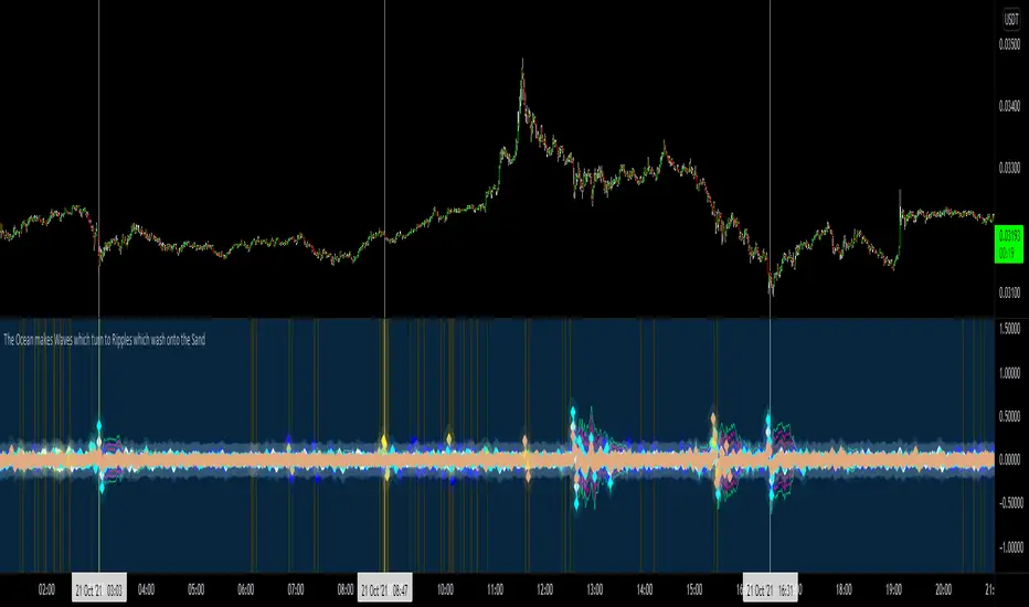
OWRS VolatilililityBit of a fun indicator taking into the asset names and natural processes and also the fact that the crypto markets are (definitely) not run by weird occultists and naturalists. Looks for disturbances in price of these four key assets. Read into it what you will. Sometimes the clues are just in the names.
Things you will learn from this script:
1. Using security function to compare multiple assets in one indicator.
2. Using indexing to reference historic data.
3. Setting chart outputs such as color based on interrogation of a boolean.
4. To only go back 3-4 iterations of any repeatable sequence as chaos kicks in after 3.55 (Feigenbaum)
1. By extension only the last 3 or 4 candles are of any use in indicator creation.
2. I am almost definitely a pagan.
3. You were expecting this numbered list to go 1,2,3,4,5,6,7. na mate. Chaos.
Combo Backtest 123 Reversal & Fractal Chaos Oscillator This is combo strategies for get a cumulative signal.
First strategy
This System was created from the Book "How I Tripled My Money In The
Futures Market" by Ulf Jensen, Page 183. This is reverse type of strategies.
The strategy buys at market, if close price is higher than the previous close
during 2 days and the meaning of 9-days Stochastic Slow Oscillator is lower than 50.
The strategy sells at market, if close price is lower than the previous close price
during 2 days and the meaning of 9-days Stochastic Fast Oscillator is higher than 50.
Second strategy
The value of Fractal Chaos Oscillator is calculated as the difference between
the most subtle movements of the market. In general, its value moves between
-1.000 and 1.000. The higher the value of the Fractal Chaos Oscillator, the
more one can say that it follows a certain trend – an increase in prices trend,
or a decrease in prices trend.
Being an indicator expressed in a numeric value, traders say that this is an
indicator that puts a value on the trendiness of the markets. When the FCO reaches
a high value, they initiate the “buy” operation, contrarily when the FCO reaches a
low value, they signal the “sell” action. This is an excellent indicator to use in
intra-day trading.
WARNING:
- For purpose educate only
- This script to change bars colors.
