BTR Auto Buy/Sell Trend System
BTR Auto Buy/Sell Trend System — Your New Profit Machine!
Discover the only TradingView system you need to spot powerful trend reversals with precision, confidence, and automation.
Designed for Stocks, Crypto & Commodities, this strategy consistently delivers 60%–80% accuracy in trending markets.
This is not just a script…
👉 It’s your complete plug-and-play trading system.
💡 Why Traders Love This System
✔ Early Trend Identification
Catch major reversals before the crowd.
✔ Non-Repainting Confirmed Signals
All entries are triggered only on candle close, so what you see is what you trade.
✔ Smart ATR + Momentum Engine
Filters bad trades automatically, giving you only high-quality signals.
✔ Works on All Timeframes
From 5-minute scalping to daily swing trading.
✔ Full Auto-Trading Ready
Pre-built JSON alerts for API Algo Trading.
No coding. No setup headache. Just copy → paste → trade.
⚡ How You Make Money With This Strategy
Step 1: Wait for Trend Flip
🔵 BUY when the system flips from bearish → bullish
🔴 SELL when it flips from bullish → bearish
Step 2: Enter on Confirmed Signal
Trade only on the bar after signal closes.
Step 3: Ride the Trend
Let the strategy take the move.
It avoids sideways markets and shines in strong trends.
Step 4: Auto Alerts (Optional)
Turn on Dhan alerts and let the system execute trades automatically.
📈 What You Can Expect (Typical Performance)
✔ 60–80% success rate in trending markets
✔ Works in Stocks, Crypto, Commodities
✔ High accuracy in 15m, 30m, 1H, 4H charts
✔ Avoids most fake breakouts & sideways noise
This system is built for consistency, simplicity, and scalable automation.
⭐ Perfect For:
Beginner traders
Algo traders
Swing traders
Scalpers
Systematic
API users
Anyone who wants clean, high-probability trend signals
⚠ Disclaimer
Trading involves risk. Past results do not guarantee future returns.
Use proper risk management for best results.
Kitaran

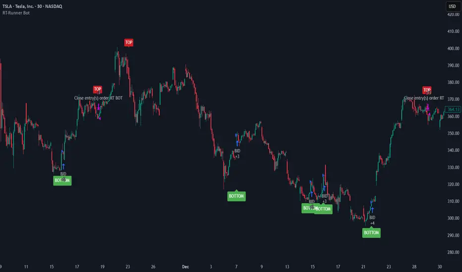
RT-Runner BotRunner Bot is a trend following tool designed to highlight when price shifts from normal back and forth rotation into stronger directional moves. It is built to help traders focus on higher quality trend legs, stay patient during chop, and avoid forcing trades when conditions are not aligned.
Blurring The Lines - Indicator vs Bot
Rainbow Trends set out to combine some of the ideas behind automated trading bots with the flexibility of trading indicators. After years of development, Runner Bot was built as an "indicator bot" that can be applied across multiple assets and multiple timeframes from the same interface.
How It Works
This tool aims to identify points where large market players - the "whales" - may be more likely to reverse the trend. It generates BOTTOM signals when its conditions suggest a potential market bottom has formed, and TOP signals when it detects that a potential top has been reached.
These signals are plotted directly on the chart so traders can visually review where Runner Bot has flagged prior tops and bottoms and compare them with their own levels, structure, and risk management.
How It Changes With Timeframe
Runner Bot identifies trend reversals based on the selected timeframe. The same logic can be applied across intraday, swing, and macro views, but its behavior will naturally change:
For macro level reversals, many traders focus on higher timeframes such as H4 to H12.
If you are scalping, you can switch to much lower timeframes, but keep in mind that bottoms detected on shorter intervals are less reliable at predicting a true long term bottom.
Choosing the timeframe intentionally is important: higher timeframes tend to highlight larger structural tops and bottoms, while lower timeframes are more sensitive to short term noise.
Tuning The Bot
Runner Bot was built to be relatively turnkey, but it does allow users to tune it for specific timeframes and assets.
To adjust the sensitivity of the TOP/BOTTOM prints, adjust the first two values in the settings column:
Decreasing these values (negative adjustments) will generally increase the number of TOP/BOTTOM signals the bot will fire.
Increasing these values will do the opposite and make TOP/BOTTOM signals less common.
This lets traders decide whether they want Runner Bot to be more selective (fewer, higher conviction style signals) or more frequent (more signals for active traders).
The trader also has the option to toggle the signals On/Off as desired. Some traders prefer to only plot TOPs and not BOTTOMs, or only BOTTOMs and not TOPs, depending on their strategy.
Limitations Of The Tool
Under the hood, Runner Bot uses internal algorithms working together to analyze price action. It can be applied across multiple timeframes, but like any tool, it has its sweet spots:
On higher ranges like 12H to 1D, you will mostly see TOP signals, which can be useful for monitoring extended moves.
On ultra low timeframes under 15 minutes, market noise can increase and short term bottoms are less reliable as long term turning points.
Fine tuning your settings to match your strategy, asset, and timeframe is recommended rather than relying on one configuration for every situation.
Preferred Settings
Over time, a few configurations have become common starting points:
H4 - A core timeframe to start catching both Tops and Bottoms across TradFi, Crypto, and Commodities.
H2/H4 Combo - Monitoring Bottoms on H2 and taking profits on H4 has been a popular combination among Rainbow Theory traders. H2 can provide earlier entries, while H4 offers a more conservative, lagging exit.
1D/H24 - Helpful for macro Tops in both TradFi and Crypto when combined with other higher timeframe context.
These are not rules, but practical examples of how some traders choose to deploy Runner Bot.
Automating Alerts
Runner Bot can also be connected to standard TradingView alerts so TOP and BOTTOM signals do not need to be watched manually on every bar.
A typical alert setup:
Symbol - Set to the asset you are charting.
Condition - Set to Runner Bot (this will use the settings you currently have on the chart).
Condition detail - Use the alert() function calls only so the tool can send alerts when TOP or BOTTOM signals fire.
Interval - Same as chart (this locks alerts to the timeframe you set them up on).
Once alerts are configured, TradingView can notify you according to your alert preferences whenever Runner Bot detects a new TOP or BOTTOM based on your current settings.
Important Note
Runner Bot is intended to provide additional context around tops, bottoms, and broader trend behavior. It is not a standalone signal generator and should always be used together with your own analysis, testing, and risk management. Historical Runner Bot signals and past market reversals do not guarantee future results.
🐋 Tight lines and happy trading!
4H Confirmation + 1H SFP BOS Retest4H Confirmation + 1H Entry (SFP + BOS + Retest)Run it on 1H
Uses 4H EMAs for higher-timeframe direction (confirmation)
Uses 1H SFP + BOS + retest + RSI for entries
This gives you more trades, still guided by the 4H trend

yangwen1.0This script is an initial concept of mine. I attempted to use the 5-minute chart as ticks for catching bottoms and picking tops, but it's unable to avoid whipsaws. I've tested many methods to evade whipsaws, but they ultimately result in poor entry points, causing me to miss the bottoms and tops of price swings. I sincerely hope someone with better approaches can discuss this with me. Thank you.

STRATEGY 1 │ Red Dragon │ Model 1 │ Pro │ [Titans_Invest]The Red Dragon Model 1 is a fully automated trading strategy designed to operate BTC/USDT.P on the 4-hour chart with precision, stability, and consistency. It was built to deliver reliable behavior even during strong market movements, maintaining operational discipline and avoiding abrupt variations that could interfere with the trader’s decision-making.
Its core is based on a professionally engineered logical structure that combines trend filters, confirmation criteria, and balanced risk management. Every component was designed to work in an integrated way, eliminating noise, avoiding unnecessary trades, and protecting capital in critical moments. There are no secret mechanisms or hidden logic: everything is built to be objective, clean, and efficient.
Even though it is based on professional quantitative engineering, Red Dragon Model 1 remains extremely simple to operate. All logic is clearly displayed and fully accessible within TradingView itself, making it easy to understand for both beginners and experienced traders. The structure is organized so that any user can quickly view entry conditions, exit criteria, additional filters, adjustable parameters, and the full mechanics behind the strategy’s behavior.
In addition, the architecture was built to minimize unnecessary complexity. Parameters are straightforward, intuitive, and operate in a balanced way without requiring deep adjustments or advanced knowledge. Traders have full freedom to analyze the strategy, understand the logic, and make personal adaptations if desired—always with total transparency inside TradingView.
The strategy was also designed to deliver consistent operational behavior over the long term. Its confirmation criteria reduce impulsive trades; its filters isolate noise; and its overall logic prioritizes high-quality entries in structured market movements. The goal is to provide a stable, clear, and repeatable flow—essential characteristics for any medium-term quantitative approach.
Combining clarity, professional structure, and ease of use, Red Dragon Model 1 offers a solid foundation both for users who want a ready-to-use automated strategy and for those looking to study quantitative models in greater depth.
This entire project was built with extreme dedication, backed by more than 14,000 hours of hands-on experience in Pine Script, continuously refining patterns, techniques, and structures until reaching its current level of maturity. Every line of code reflects this long process of improvement, resulting in a strategy that unites professional engineering, transparency, accessibility, and reliable execution.
🔶 MAIN FEATURES
• Fully automated and robust: Operates without manual intervention, ideal for traders seeking consistency and stability. It delivers reliable performance even in volatile markets thanks to the solid quantitative engineering behind the system.
• Multiple layers of confirmation: Combines 10 key technical indicators with 15 adaptive filters to avoid false signals. It only triggers entries when all trend, market strength, and contextual criteria align.
• Configurable and adaptable filters: Each of the 15 filters can be enabled, disabled, or adjusted by the user, allowing the creation of personalized statistical models for different assets and timeframes. This flexibility gives full freedom to optimize the strategy according to individual preferences.
• Clear and accessible logic: All entry and exit conditions are explicitly shown within the TradingView parameters. The strategy has no hidden components—any user can quickly analyze and understand each part of the system.
• Integrated exclusive tools: Includes complete backtest tables (desktop and mobile versions) with annualized statistics, along with real-time entry conditions displayed directly on the chart. These tools help monitor the strategy across devices and track performance and risk metrics.
• No repaint: All signals are static and do not change after being plotted. This ensures the trader can trust every entry shown without worrying about indicators rewriting past values.
🔷 ENTRY CONDITIONS & RISK MANAGEMENT
Red Dragon Model 1 triggers buy (long) or sell (short) signals only when all configured conditions are satisfied. For example:
• Volume:
• The system only trades when current volume exceeds the volume moving average multiplied by a user-defined factor, indicating meaningful market participation.
• RSI:
• Confirms bullish bias when RSI crosses above its moving average, and bearish bias when crossing below.
• ADX:
• Enters long when +DI is above –DI with ADX above a defined threshold, indicating directional strength to the upside (and the opposite conditions for shorts).
• Other indicators (MACD, SAR, Ichimoku, Support/Resistance, etc.)
Each one must confirm the expected direction before a final signal is allowed.
When all bullish criteria are met simultaneously, the system enters Long; when all criteria indicate a bearish environment, the system enters Short.
In addition, the strategy uses fixed Take Profit and Stop Loss targets for risk control:
Currently: TP around 1.5% and SL around 2.0% per trade, ensuring consistent and transparent risk management on every position.
⚙️ INDICATORS
__________________________________________________________
1) 🔊 Volume: Avoids trading on flat charts.
2) 🍟 MACD: Tracks momentum through moving averages.
3) 🧲 RSI: Indicates overbought or oversold conditions.
4) 🅰️ ADX: Measures trend strength and potential entry points.
5) 🥊 SAR: Identifies changes in price direction.
6) ☁️ Cloud: Accurately detects changes in market trends.
7) 🌡️ R/F: Improves trend visualization and helps avoid pitfalls.
8) 📐 S/R: Fixed support and resistance levels.
9)╭╯MA: Moving Averages.
10) 🔮 LR: Forecasting using Linear Regression.
__________________________________________________________
🟢 ENTRY CONDITIONS 🔴
__________________________________________________________
IF all conditions are 🟢 = 📈 Long
IF all conditions are 🔴 = 📉 Short
__________________________________________________________
🚨 CURRENT TRIGGER SIGNAL 🚨
__________________________________________________________
🔊 Volume
🟢 LONG = (volume) > (MA_volume) * (Volume Mult)
🔴 SHORT = (volume) > (MA_volume) * (Volume Mult)
🧲 RSI
🟢 LONG = (RSI) > (RSI_MA)
🔴 SHORT = (RSI) < (RSI_MA)
🟢 ALL ENTRY CONDITIONS AVAILABLE 🔴
__________________________________________________________
🔊 Volume
🟢 LONG = (volume) > (MA_volume) * (Volume Mult)
🔴 SHORT = (volume) > (MA_volume) * (Volume Mult)
🔊 Volume
🟢 LONG = (volume) > (MA_volume) * (Volume Mult) and (close) > (open)
🔴 SHORT = (volume) > (MA_volume) * (Volume Mult) and (close) < (open)
🍟 MACD
🟢 LONG = (MACD) > (Signal Smoothing)
🔴 SHORT = (MACD) < (Signal Smoothing)
🧲 RSI
🟢 LONG = (RSI) < (Upper)
🔴 SHORT = (RSI) > (Lower)
🧲 RSI
🟢 LONG = (RSI) > (RSI_MA)
🔴 SHORT = (RSI) < (RSI_MA)
🅰️ ADX
🟢 LONG = (+DI) > (-DI) and (ADX) > (Treshold)
🔴 SHORT = (+DI) < (-DI) and (ADX) > (Treshold)
🥊 SAR
🟢 LONG = (close) > (SAR)
🔴 SHORT = (close) < (SAR)
☁️ Cloud
🟢 LONG = (Cloud A) > (Cloud B)
🔴 SHORT = (Cloud A) < (Cloud B)
☁️ Cloud
🟢 LONG = (Kama) > (Kama )
🔴 SHORT = (Kama) < (Kama )
🌡️ R/F
🟢 LONG = (high) > (UP Range) and (upward) > (0)
🔴 SHORT = (low) < (DOWN Range) and (downward) > (0)
🌡️ R/F
🟢 LONG = (high) > (UP Range)
🔴 SHORT = (low) < (DOWN Range)
📐 S/R
🟢 LONG = (close) > (Resistance)
🔴 SHORT = (close) < (Support)
╭╯MA2️⃣
🟢 LONG = (Cyan Bar MA2️⃣)
🔴 SHORT = (Red Bar MA2️⃣)
╭╯MA2️⃣
🟢 LONG = (close) > (MA2️⃣)
🔴 SHORT = (close) < (MA2️⃣)
╭╯MA2️⃣
🟢 LONG = (Positive MA2️⃣)
🔴 SHORT = (Negative MA2️⃣)
__________________________________________________________
🎯 TP / SL 🛑
__________________________________________________________
🎯 TP: 1.5 %
🛑 SL: 2.0 %
__________________________________________________________
🪄 UNIQUE FEATURES OF THIS STRATEGY
____________________________________
1) 𝄜 Table Backtest for Mobile.
2) 𝄜 Table Backtest for Computer.
3) 𝄜 Table Backtest for Computer & Annual Performance.
4) 𝄜 Live Entry Conditions.
1) 𝄜 Table Backtest for Mobile.
2) 𝄜 Table Backtest for Computer.
3) 𝄜 Table Backtest for Computer & Annual Performance.
4) 𝄜 Live Entry Conditions.
_____________________________
𝄜 BACKTEST / PERFORMANCE 𝄜
_____________________________
• Net Profit: +634.47%, Maximum Drawdown: -18.44%.
🪙 PAIR / TIMEFRAME ⏳
🪙 PAIR: BINANCE:BTCUSDT.P
⏳ TIME: 4 hours (240m)
✅ ON ☑️ OFF
✅ LONG
✅ SHORT
🎯 TP / SL 🛑
🎯 TP: 1.5 (%)
🛑 SL: 2.0 (%)
⚙️ CAPITAL MANAGEMENT
💸 Initial Capital: 10000 $ (TradingView)
💲 Order Size: 10 % (Of Equity)
🚀 Leverage: 10 x (Exchange)
💩 Commission: 0.03 % (Exchange)
📆 BACKTEST
🗓️ Start: Setember 24, 2019
🗓️ End: November 21, 2025
🗓️ Days: 2250
🗓️ Yers: 6.17
🗓️ Bars: 13502
📊 PERFORMANCE
💲 Net Profit: + 63446.89 $
🟢 Net Profit: + 634.47 %
💲 DrawDown Maximum: - 10727.48 $
🔴 DrawDown Maximum: - 18.44 %
🟢 Total Closed Trades: 1042
🟡 Percent Profitable: 63.92 %
🟡 Profit Factor: 1.247
💲 Avg Trade: + 60.89 $
⏱️ Avg # Bars in Trades
🕯️ Avg # Bars: 4
⏳ Avg # Hrs: 15
✔️ Trades Winning: 666
❌ Trades Losing: 376
✔️ Maximum Consecutive Wins: 11
❌ Maximum Consecutive Losses: 7
📺 Live Performance : br.tradingview.com
• Use this strategy on the recommended pair and timeframe above to replicate the tested results.
• Feel free to experiment and explore other settings, assets, and timeframes.

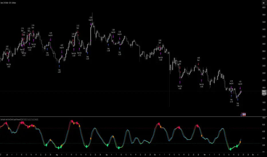
Stochastic Hash Strat [Hash Capital Research]# Stochastic Hash Strategy by Hash Capital Research
## 🎯 What Is This Strategy?
The **Stochastic Slow Strategy** is a momentum-based trading system that identifies oversold and overbought market conditions to capture mean-reversion opportunities. Think of it as a "buy low, sell high" approach with smart mathematical filters that remove emotion from your trading decisions.
Unlike fast-moving indicators that generate excessive noise, this strategy uses **smoothed stochastic oscillators** to identify only the highest-probability setups when momentum truly shifts.
---
## 💡 Why This Strategy Works
Most traders fail because they:
- **Chase prices** after big moves (buying high, selling low)
- **Overtrade** in choppy, directionless markets
- **Exit too early** or hold losses too long
This strategy solves all three problems:
1. **Entry Discipline**: Only trades when the stochastic oscillator crosses in extreme zones (oversold for longs, overbought for shorts)
2. **Cooldown Filter**: Prevents revenge trading by forcing a waiting period after each trade
3. **Fixed Risk/Reward**: Pre-defined stop-loss and take-profit levels ensure consistent risk management
**The Math Behind It**: The stochastic oscillator measures where the current price sits relative to its recent high-low range. When it's below 25, the market is oversold (time to buy). When above 70, it's overbought (time to sell). The crossover with its moving average confirms momentum is shifting.
---
## 📊 Best Markets & Timeframes
### ⭐ OPTIMAL PERFORMANCE:
**Crude Oil (WTI) - 12H Timeframe**
- **Why it works**: Oil markets have predictable volatility patterns and respect technical levels
**AAVE/USD - 4H to 12H Timeframe**
- **Why it works**: DeFi tokens exhibit strong momentum cycles with clear extremes
### ✅ Also Works Well On:
- **BTC/USD** (12H, Daily) - Lower frequency but high win rate
- **ETH/USD** (8H, 12H) - Balanced volatility and liquidity
- **Gold (XAU/USD)** (Daily) - Classic mean-reversion asset
- **EUR/USD** (4H, 8H) - Lower volatility, requires patience
### ❌ Avoid Using On:
- Timeframes below 4H (too much noise)
- Low-liquidity altcoins (wide spreads kill performance)
- Strongly trending markets without pullbacks (Bitcoin in 2021)
- News-driven instruments during major events
---
## 🎛️ Understanding The Settings
### Core Stochastic Parameters
**Stochastic Length (Default: 16)**
- Controls the lookback period for price comparison
- Lower = faster reactions, more signals (10-14 for volatile markets)
- Higher = smoother signals, fewer trades (16-21 for stable markets)
- **Pro tip**: Use 10 for crypto 4H, 16 for commodities 12H
**Overbought Level (Default: 70)**
- Threshold for short entries
- Lower values (65-70) = more trades, earlier entries
- Higher values (75-80) = fewer but higher-conviction trades
- **Sweet spot**: 70 works for most assets
**Oversold Level (Default: 25)**
- Threshold for long entries
- Higher values (25-30) = more trades, earlier entries
- Lower values (15-20) = fewer but stronger bounce setups
- **Sweet spot**: 20-25 depending on market conditions
**Smooth K & Smooth D (Default: 7 & 3)**
- Additional smoothing to filter out whipsaws
- K=7 makes the indicator slower and more reliable
- D=3 is the signal line that confirms the trend
- **Don't change these unless you know what you're doing**
---
### Risk Management
**Stop Loss % (Default: 2.2%)**
- Automatically exits losing trades
- Should be 1.5x to 2x your average market volatility
- Too tight = death by a thousand cuts
- Too wide = uncontrolled losses
- **Calibration**: Check ATR indicator and set SL slightly above it
**Take Profit % (Default: 7%)**
- Automatically exits winning trades
- Should be 2.5x to 3x your stop loss (reward-to-risk ratio)
- This default gives 7% / 2.2% = 3.18:1 R:R
- **The golden rule**: Never have R:R below 2:1
---
### Trade Filters
**Bar Cooldown Filter (Default: ON, 3 bars)**
- **What it does**: Forces you to wait X bars after closing a trade before entering a new one
- **Why it matters**: Prevents emotional revenge trading and overtrading in choppy markets
- **Settings guide**:
- 3 bars = Standard (good for most cases)
- 5-7 bars = Conservative (oil, slow-moving assets)
- 1-2 bars = Aggressive (only for experienced traders)
**Exit on Opposite Extreme (Default: ON)**
- Closes your long when stochastic hits overbought (and vice versa)
- Acts as an early profit-taking mechanism
- **Leave this ON** unless you're testing other exit strategies
**Divergence Filter (Default: OFF)**
- Looks for price/momentum divergences for additional confirmation
- **When to enable**: Trending markets where you want fewer but higher-quality trades
- **Keep OFF for**: Mean-reverting markets (oil, forex, most of the time)
---
## 🚀 Quick Start Guide
### Step 1: Set Up in TradingView
1. Open TradingView and navigate to your chart
2. Click "Pine Editor" at the bottom
3. Copy and paste the strategy code
4. Click "Add to Chart"
5. The strategy will appear in a separate pane below your price chart
### Step 2: Choose Your Market
**If you're trading Crude Oil:**
- Timeframe: 12H
- Keep all default settings
- Watch for signals during London/NY overlap (8am-11am EST)
**If you're trading AAVE or crypto:**
- Timeframe: 4H or 12H
- Consider these adjustments:
- Stochastic Length: 10-14 (faster)
- Oversold: 20 (more aggressive)
- Take Profit: 8-10% (higher targets)
### Step 3: Wait for Your First Signal
**LONG Entry** (Green circle appears):
- Stochastic crosses up below oversold level (25)
- Price likely near recent lows
- System places limit order at take profit and stop loss
**SHORT Entry** (Red circle appears):
- Stochastic crosses down above overbought level (70)
- Price likely near recent highs
- System places limit order at take profit and stop loss
**EXIT** (Orange circle):
- Position closes either at stop, target, or opposite extreme
- Cooldown period begins
### Step 4: Let It Run
The biggest mistake? **Interfering with the system.**
- Don't close trades early because you're scared
- Don't skip signals because you "have a feeling"
- Don't increase position size after a big win
- Don't revenge trade after a loss
**Follow the system or don't use it at all.**
---
### Important Risks:
1. **Drawdown Pain**: You WILL experience losing streaks of 5-7 trades. This is mathematically normal.
2. **Whipsaw Markets**: Choppy, range-bound conditions can trigger multiple small losses.
3. **Gap Risk**: Overnight gaps can cause your actual fill to be worse than the stop loss.
4. **Slippage**: Real execution prices differ from backtested prices (factor in 0.1-0.2% slippage).
---
## 🔧 Optimization Guide
### When to Adjust Settings:
**Market Volatility Increased?**
- Widen stop loss by 0.5-1%
- Increase take profit proportionally
- Consider increasing cooldown to 5-7 bars
**Getting Too Few Signals?**
- Decrease stochastic length to 10-12
- Increase oversold to 30, decrease overbought to 65
- Reduce cooldown to 2 bars
**Getting Too Many Losses?**
- Increase stochastic length to 18-21 (slower, smoother)
- Enable divergence filter
- Increase cooldown to 5+ bars
- Verify you're on the right timeframe
### A/B Testing Method:
1. **Run default settings for 50 trades** on your chosen market
2. Document: Win rate, profit factor, max drawdown, emotional tolerance
3. **Change ONE variable** (e.g., oversold from 25 to 20)
4. Run another 50 trades
5. Compare results
6. Keep the better version
**Never change multiple settings at once** or you won't know what worked.
---
## 📚 Educational Resources
### Key Concepts to Learn:
**Stochastic Oscillator**
- Developed by George Lane in the 1950s
- Measures momentum by comparing closing price to price range
- Formula: %K = (Close - Low) / (High - Low) × 100
- Similar to RSI but more sensitive to price movements
**Mean Reversion vs. Trend Following**
- This is a **mean reversion** strategy (price returns to average)
- Works best in ranging markets with defined support/resistance
- Fails in strong trending markets (2017 Bitcoin, 2020 Tech stocks)
- Complement with trend filters for better results
**Risk:Reward Ratio**
- The cornerstone of profitable trading
- Winning 40% of trades with 3:1 R:R = profitable
- Winning 60% of trades with 1:1 R:R = breakeven (after fees)
- **This strategy aims for 45% win rate with 2.5-3:1 R:R**
### Recommended Reading:
- *"Trading Systems and Methods"* by Perry Kaufman (Chapter on Oscillators)
- *"Mean Reversion Trading Systems"* by Howard Bandy
- *"The New Trading for a Living"* by Dr. Alexander Elder
---
## 🛠️ Troubleshooting
### "I'm not seeing any signals!"
**Check:**
- Is your timeframe 4H or higher?
- Is the stochastic actually reaching extreme levels (check if your asset is stuck in middle range)?
- Is cooldown still active from a previous trade?
- Are you on a low-liquidity pair?
**Solution**: Switch to a more volatile asset or lower the overbought/oversold thresholds.
---
### "The strategy keeps losing money!"
**Check:**
- What's your win rate? (Below 35% is concerning)
- What's your profit factor? (Below 0.8 means serious issues)
- Are you trading during major news events?
- Is the market in a strong trend?
**Solution**:
1. Verify you're using recommended markets/timeframes
2. Increase cooldown period to avoid choppy markets
3. Reduce position size to 5% while you diagnose
4. Consider switching to daily timeframe for less noise
---
### "My stop losses keep getting hit!"
**Check:**
- Is your stop loss tighter than the average ATR?
- Are you trading during high-volatility sessions?
- Is slippage eating into your buffer?
**Solution**:
1. Calculate the 14-period ATR
2. Set stop loss to 1.5x the ATR value
3. Avoid trading right after market open or major news
4. Factor in 0.2% slippage for crypto, 0.1% for oil
---
## 💪 Pro Tips from the Trenches
### Psychological Discipline
**The Three Deadly Sins:**
1. **Skipping signals** - "This one doesn't feel right"
2. **Early exits** - "I'll just take profit here to be safe"
3. **Revenge trading** - "I need to make back that loss NOW"
**The Solution:** Treat your strategy like a business system. Would McDonald's skip making fries because the cashier "doesn't feel like it today"? No. Systems work because of consistency.
---
### Position Management
**Scaling In/Out** (Advanced)
- Enter 50% position at signal
- Add 50% if stochastic reaches 10 (oversold) or 90 (overbought)
- Exit 50% at 1.5x take profit, let the rest run
**This is NOT for beginners.** Master the basic system first.
---
### Market Awareness
**Oil Traders:**
- OPEC meetings = volatility spikes (avoid or widen stops)
- US inventory reports (Wed 10:30am EST) = avoid trading 2 hours before/after
- Summer driving season = different patterns than winter
**Crypto Traders:**
- Monday-Tuesday = typically lower volatility (fewer signals)
- Thursday-Sunday = higher volatility (more signals)
- Avoid trading during exchange maintenance windows
---
## ⚖️ Legal Disclaimer
This trading strategy is provided for **educational purposes only**.
- Past performance does not guarantee future results
- Trading involves substantial risk of loss
- Only trade with capital you can afford to lose
- No one associated with this strategy is a licensed financial advisor
- You are solely responsible for your trading decisions
**By using this strategy, you acknowledge that you understand and accept these risks.**
---
## 🙏 Acknowledgments
Strategy development inspired by:
- George Lane's original Stochastic Oscillator work
- Modern quantitative trading research
- Community feedback from hundreds of backtests
Built with ❤️ for retail traders who want systematic, disciplined approaches to the markets.
---
**Good luck, stay disciplined, and trade the system, not your emotions.**
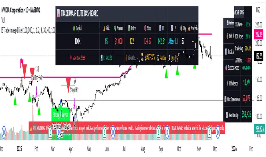
Tradermaap Elite System [Institutional Grade Analysis]Description:
🚀 Institutional Trend Modeling & Automated Risk Engine
Tradermaap Elite is a proprietary quantitative trading system designed for professional scalpers, swing traders, and prop firm challengers. It moves beyond standard indicators by utilizing a Dynamic Mean Reversion Algorithm to identify high-probability structural turning points in the market.
This is NOT just a buy/sell arrow tool. It is a complete Decision Support System that mathematically calculates your risk, entry, and exit zones based on institutional order flow concepts.
🛠️ Key Features
✅ 100% Non-Repainting Engine: Signals are locked on candle close. No disappearing acts. ✅ Institutional Baseline Logic: Uses a proprietary blend of long-term trend filters to avoid false signals in choppy markets. ✅ Auto Risk Guard: Automatically calculates Position Size based on your account balance and defined risk (1% Prop Mode). ✅ Multi-Asset Calibration: Algorithmically tuned for Bitcoin, Gold, Indices (US30/NAS100), and Equities. ✅ Live Dashboard: Tracks real-time Win Rate and Profit Factor directly on your chart. ✅ Dynamic Currency: Switch between USD ($) and INR (₹) in settings.
🧠 How It Works (The Logic)
The system operates on a 3-Stage "Confluence" Mechanism:
Macro Trend Identification: The algorithm scans for the dominant market direction using a Weighted Trend Filter.
Equilibrium Reversion: It identifies when price is "overextended" and waits for it to return to the "Value Zone" (Discount/Premium levels).
Volatility Trigger: A trade is only validated when specific volume and price action conditions are met, filtering out weak moves.
Projected Outcomes:
Protective Stop: Structure-based invalidation levels.
Target 1: Conservative banking zones.
Target 2: Trend-following extensions.
🔒 Access & Licensing
This operates as a Protected Algorithm. It is strictly Invite-Only. To obtain a license key or start a trial, please refer to the link in the signature below.
⚠️ RISK DISCLAIMER: This script is for educational and chart analysis purposes only. It incorporates mathematical modeling to assist in decision-making but does not guarantee profits. Trading is inherently risky. Use responsibly.
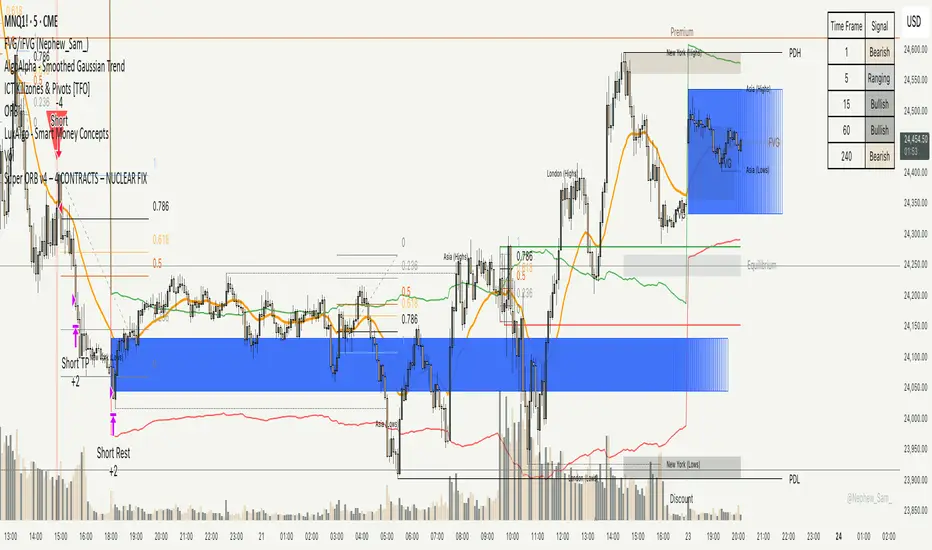
Super ORB v4 – 4 CONTRACTS – NUCLEAR FIXORB hands off printer, this is to gauge how few trades can happen off the ORB while not trading after hours either. Should be in the 5% a month range 4 contracts, no more than 5 trades a month.
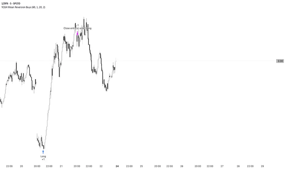
YCGH Mean Reversion StrategyThis strategy applies a classic mean-reversion framework inspired by the concepts popularized by Ernest P. Chan in his quantitative trading books.
It uses Bollinger Bands and RSI to identify statistically stretched conditions where price has moved too far from its average. When price dips below the lower band with weakening momentum, the strategy accumulates small long positions, expecting reversion toward the mean. As price rebounds above the upper band, it exits positions gradually. Position sizing limits help control risk and avoid excessive exposure.
Special thanks to Ernest P. Chan for his influential work in quantitative trading, which motivated the structure and logic behind this model.
BTC Risk Metric DCA Adapter (3Commas Webhook Strategy)Risk Metric DCA Adapter (3Commas Webhook Strategy) - WORK IN PROGRESS
This Pine Script strategy, originally inspired by the Risk Metric Indicator, is fundamentally engineered as an Adapter to interface with external trading bots like 3Commas via Webhooks. It calculates a dynamic market risk score and translates that score into specific dollar-cost averaging (DCA) entry levels and tiered profit-taking exits.
Key Features & Logic
Risk Metric Calculation (Credit to The Trading Parrot):
The strategy incorporates a complex, multi-timeframe Risk Metric calculation based on daily and weekly moving averages (SMA) and standard deviation (StDev). This metric aims to quantify the current market overextension or compression relative to long-term historical data. The resulting score dictates the level of conviction for a new trade.
Tiered DCA Entry Sizing:
The strategy defines three distinct Buy Levels (L1, L2, L3) corresponding to increasingly favorable (lower) Risk Metric scores.
L1 (Base): Risk is moderate, initiating the minimum defined trade amount.
L2 (Scaled): Risk is low, initiating L1 amount + L2 amount.
L3 (Aggressive): Risk is very low, initiating L1 + L2 + L3 amounts.
Tiered Profit-Taking Exits:
The strategy implements a staggered, partial profit-taking approach based on the Risk Metric rising:
Sell L1 & L2: Closes a percentage of the current position when the Risk Metric reaches defined high thresholds, locking in partial profits.
Sell L3 (Full Exit): Closes the remaining position when the Risk Metric reaches the highest defined threshold.
The Adapter Function (Webhook Integration)
This script is unique because it uses the Pine Script strategy() function to trigger Order Fills, which are necessary to access powerful placeholders in the TradingView alert system.
Trigger Type: The alert must be set to trigger on Any order fill.
Dynamic Webhook Data: Instead of using fixed alert() commands, the strategy generates dynamic labels (e.g., BUY_ENTRY_L3_USD_1000 or SELL_L1_PCT_25) using the strategy.entry and strategy.close commands.
Data Transfer: The alert message then uses the placeholder {{strategy.order.comment}} to pass these dynamic labels to the 3Commas bot, allowing the bot to execute the precise action (e.g., start_deal_with_volume_in_quote_currency or close_deal_at_market_percentage).
Full Strategy Webhook payload
{
"secret": "YOUR_3COMMAS_SECRET_KEY",
"max_lag": "300",
"timestamp": "{{timenow}}",
"trigger_price": "{{close}}",
"tv_exchange": "{{exchange}}",
"tv_instrument": "{{ticker}}",
"action": "{{strategy.order.action}}",
"bot_uuid": "YOUR_BOT_UUID",
"strategy_info": {
"market_position": "{{strategy.market_position}}",
"market_position_size": "{{strategy.market_position_size}}",
"prev_market_position": "{{strategy.prev_market_position}}",
"prev_market_position_size": "{{strategy.prev_market_position_size}}"
},
"order": {
"amount": "{{strategy.order.contracts}}",
"currency_type": "base",
"comment": "{{strategy.order.comment}}"
}
}
Disclaimer: This script is an adapter tool and does not guarantee profit. Trading requires manual configuration of risk settings, bot parameters, and adherence to platform-specific setup instructions.

V15.0 Adaptive Chameleon [Pro]
# **V15.0 Adaptive Chameleon – Strategy Description**
**Adaptive Chameleon** is a fully automated TradingView strategy powered by a signal engine based on multi-timeframe trend analysis, adaptive moving averages, and a volatility filter. The goal is to trade in the direction of a strong and confirmed trend, avoid opening trades in weak or manipulative price zones, and establish positions with a clearly defined risk/reward ratio.
---
## **1. General Logic and Philosophy**
The strategy divides tasks between two timeframes:
* **4-Hour Chart → Trend Manager (Boss)**
Determines the direction and strength of the trend.
* **4-Minute Chart → Entry Trigger (Operating Unit)**
Generates the ideal entry signal in the direction of the trend.
Thanks to this structure, the strategy both follows the long-term main direction and finds clear entries with low lag on smaller timeframes.
---
## **2. Trend Detection (4H)**
The strategy uses **KAMA (Kaufman Adaptive Moving Average)** and **ADX** to identify trends on the higher timeframe.
### **KAMA – Adaptive Trend Line**
* The KAMA is much more "smart" than traditional moving averages.
* It accelerates during price movements and decelerates during sideways movements.
* This allows for much clearer detection of trend direction.
### **ADX – Trend Strength Meter**
The strategy only opens trades when **trend strength** is rising (above the ADX average).
This prevents unnecessary trades when the trend is weak.
### **Trend Rules**
* Price above the KAMA → **Uptrend**
* Price below the KAMA → **Downtrend**
* ADX widening → **Trend strong**
The entry trigger is activated when these three conditions are met together.
---
## **3. Entry Engine (45m)**
On the 45-minute timeframe, the system uses the following components:
### **AlphaTrend (MFI + ATR-Based Adaptive Line)**
* Measures market flow direction with MFI (Money Flow Index),
* Measures price level breakouts with ATR (Volatility).
AlphaTrend detects whether the price is likely to reverse upwards or downwards.
### **Entry Signal**
* **Buy signal:** If the AlphaTrend has reversed upwards based on recent bars
* **Sell signal:** If the AlphaTrend has broken downwards
### **Pivot Points (For Stop)**
* The **pivotLow** and **pivotHigh** levels of the last 10 bars are calculated.
* These are used to determine the most logical stop distance.
---
## **4. Protection Shields**
The strategy uses two main filters to protect against the most dangerous conditions in the crypto market:
### **1. Pump/Dump Filter**
* A candlestick length greater than 4% is considered a "pump bar."
* Never open a trade on these bars.
The goal: to avoid sudden manipulation candlesticks.
### **2. RSI Filter**
* Long trades: RSI > 45 (open long on weak momentum)
* Short trades: RSI < 55 (open short on extremely strong momentum)
These filters provide more balanced entries.
---
## **5. Final Entry Conditions**
### **All conditions are required simultaneously for long:**
1. 4H trend up
2. ADX trend strength increasing
3. 45m AlphaTrend issued a "buy" signal
4. RSI > 45
5. No candlestick pump
6. Date range is suitable
### **All conditions apply in the opposite direction for short.**
---
## **6. Exit Mechanism (Stop, TP, Trailing)**
The strategy uses a three-layer structure on the exit side:
### **1. Pivot-Based Stop**
* Stop distance = Entry price − Pivot Low (for long)
* Minimum stop distance = **1% of the price**
Provides both structural and mathematical security.
### **2. Fixed R:R (Default 1:2)**
* TP = Entry + Stop Distance × R:R
The default 2R target is ideal for trend systems.
### **3. Optional Trailing Stop**
* Dynamic trailing stop that follows the price by a certain percentage.
* Allows trend trades to yield greater profits.
---
## **7. Chart Displays**
* Purple line:** 4H WEDGE (main trend line)
* Yellow background:** Pump protection is active (trades will not be opened on that bar)
---
## **8. Practical Effect of the Strategy**
This system has an adaptive structure based on trend variations.
**Strengths:**
* Very high accuracy (76–80% in SOL and ETH tests)
* Low drawdown (approximately 6–7%)
* Safe entries thanks to pump/dump and extreme momentum filters
* Clearly defined stop and target structure
* Low noise thanks to multi-timeframe compatibility
**Weaknesses:**
* Performance may decrease in sideways markets without trends
* Overtrading may occur if the ADX filter is closed
* Very small stops can sometimes cause unnecessary triggers
---
## **9. Conclusion**
**Adaptive Chameleon** is a trend-based and highly stable strategy with well-established risk management, manipulation filtering, and entry into lower timeframes with clear trend direction detection and low-latency signals.
SOL and ETH demonstrated strong and balanced performance in backtests with metrics such as:
* **600+ trades**
* **30–37% profit**
* **76–80% win rate**
* **Low max drawdown**

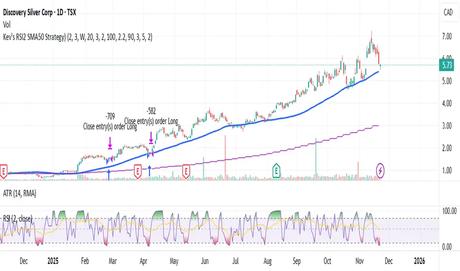
Kev's RSI2 SMA50 Strategy⭐ Kev’s RSI2 SMA50 Strategy — Institutional Edition (TSX Optimized + RR Filter)
A professional swing-trading system based on Larry Connors’ RSI(2) mean-reversion framework, optimized for TSX equities. Designed for Daily timeframe trading with institutional trend alignment, volatility filtering, and strict risk-reward controls.
📌 Overview
This strategy enhances the classic RSI(2) setup with:
• Strong trend confirmation (SMA50 + Weekly SMA50)
• Deep pullback detection (RSI2 < 3)
• Structural swing-based stop-loss
• Fixed 2R profit target (non-repainting)
• Optional Connors RSI (CRSI) confirmation
• Volatility filtering via ATR range
• Mechanical, deterministic, no-discretion rules
Works best on TSX large & mid-caps, ETFs, and liquid equities.
🔍 Core Philosophy
Buy strong stocks on pullbacks → Price must be above SMA50 + Weekly SMA50.
Pullback must be statistically meaningful → RSI(2) < 3.
R:R must justify the trade → Swing-low SL + 2R target with structural room to hit TP.
🧠 Entry Conditions (Non-Repainting)
• RSI(2) < 3 → Identifies extreme short-term oversold dips.
• SMA50 Filter → Ensures uptrend alignment.
• Weekly HTF Filter (Default = 1W) → Confirms broader trend direction.
• ATR Filter → Rejects volatile bars (range < ATR(14) × 2.2).
• Optional:
– SMA50 Slope (positive trend strength)
– Bullish Reversal Candle
– Connors RSI < 20 (deep pullback confirmation)
🎯 Risk Management
All levels are locked at entry and never repaint.
• Swing-Low SL (last 5 bars)
• 2R Profit Target = Entry + (Risk × 2)
• R:R Feasibility Filter → Only enters if recent swing high is above TP.
• Optional RSI Exit → Exit when RSI2 > 90 (enabled by default).
• Optional SMA Exit (disabled by default) → Conservative early exit.
📈 Visuals
The script plots:
• SMA50
• Weekly SMA50
• Swing-Low SL (fixed)
• 2R TP (fixed)
• Optional SMA exit line
All are non-repainting and update only on confirmed bars.
🔔 Alerts
Buy Signal → All entry filters aligned (RSI2, SMA50, HTF, ATR, RR check).
Exit Signal → 2R hit, SL hit, RSI exit, or SMA exit (if enabled).
🧭 Recommended Usage
• Timeframe: Daily
• HTF: Weekly (default)
• Best For: TSX equities, mid/large-cap stocks, ETFs
• Style: Short-term swing trading (1–10 bars)
• Avoid: Low-volume tickers, microcaps, crypto, biotech, news-driven spikes.
🛑 Notes
• All HTF data uses lookahead_off → non-repainting.
• Rules are fully mechanical and deterministic.
• Position sizing uses % equity by default.
• This script is for educational purposes only and not financial advice.
• Always forward-test before using live capital.
VIX Counter-Trend StrategyVIX Panic Index VOO Bottom-Fishing Strategy
📊 Strategy Overview
This strategy utilizes the VIX (Volatility Index) as a market sentiment indicator to help investors rationally enter positions during periods of extreme market panic, using objective technical signals to avoid emotional decision-making. It is designed to capture rebound opportunities in VOO (or other US equity ETFs) following panic-driven selloffs.
🎯 Entry and Exit Conditions
Entry Conditions (both must be met):
VIX reaches or exceeds the set threshold (default 25, adjustable)
VIX death crosses below its moving average (default 5-day MA), confirming panic sentiment is beginning to recede
Exit Conditions (three modes available):
Holding Period Mode: Exit after holding for the set number of days (default 100 days)
VIX Decline Mode: Exit when VIX falls below the set threshold (default 20)
Either Condition Mode: Exit when either condition is met
⚠️ Important Warnings
Not Suitable for Leveraged ETF Bottom-Fishing: VIX reflects market volatility. Using leveraged ETFs (such as TQQQ, SOXL) increases risk due to decay effects and greater volatility, potentially causing larger losses during panic periods.
Bear Market Inaccuracy Risk: This strategy assumes markets will rebound from panic. However, during prolonged bear markets or systemic risks (such as the 2008 financial crisis or 2022 rate hike cycle), VIX may remain elevated for extended periods, triggering multiple buy signals while prices continue declining, rendering the strategy ineffective.
Recommended to Combine with Market Trend Analysis: Works better in bull market conditions. In bear markets, consider raising VIX thresholds or suspending use.
For Reference Only, Not Investment Advice: Historical performance does not guarantee future results. Please use cautiously according to your personal risk tolerance.
VIX 恐慌指數 VOO 抄底策略
📊 策略目的
本策略利用 VIX 恐慌指數作為市場情緒指標,幫助投資人在市場極度恐慌時理性進場抄底,並透過客觀的技術訊號避免情緒化操作。適合用於捕捉 VOO(或其他美股 ETF)在恐慌性下跌後的反彈機會。
🎯 進出場條件
進場條件(同時滿足):
VIX 指數達到設定門檻以上(預設 25,可調整)
VIX 死亡交叉其均線(預設 5 日均線),確認恐慌情緒開始回落
出場條件(三種模式可選):
持有天數模式:持有達到設定天數後出場(預設 100 天)
VIX 回落模式:VIX 降至設定門檻以下時出場(預設 20)
兩者皆可模式:任一條件滿足即出場
⚠️ 重要警語
不適合槓桿型 ETF 抄底:VIX 反映的是市場波動度,使用槓桿 ETF(如 TQQQ、SOXL)會因為衰減效應和更大波動而增加風險,可能在恐慌期間造成更大虧損。
空頭市場失準風險:本策略假設市場會從恐慌中反彈,但在長期空頭或系統性風險(如 2008 金融危機、2022 升息循環)中,VIX 可能長期處於高檔,多次觸發買入訊號卻持續下跌,導致策略失效。
建議搭配大盤趨勢判斷:在多頭格局中使用效果較佳,空頭格局建議提高 VIX 門檻或暫停使用。
僅供參考,非投資建議:歷史績效不代表未來表現,請依個人風險承受度謹慎使用。

Mir Khans QQQThis strategy is built around how I actually trade QQQ intraday: Opening-Range continuation, VWAP trend reads, OI magnets, and a simple but strict risk framework. It’s designed to keep you on the right side of the session theme (trend vs fade), then only take trades when multiple pieces of confluence line up.
The strategy is tuned for QQQ on intraday timeframes, but the logic is generic enough to experiment with other liquid index products. It’s not financial advice—use it as a structured framework for reading OR, VWAP, and trend strength, and then layer your own execution rules and risk management on top.
Macketings 1min ScalpingThis is a hyper-reactive scalping strategy designed for the 1-minute chart. It utilizes a strict four-EMA hierarchy (80/90/340/500) to ensure trades are only taken in the strongest aligned market trend. The strategy is built to be extremely tight on risk and focuses on capturing the immediate, high-momentum swing that follows a confirmed EMA retest or breakout.
Key Mechanics (How it Works):
Strict Trend Alignment: Entry is only permitted when the faster EMA band (80/90) and the price action are correctly aligned with the slow trend (340/500).
Long: EMA 80/90 must be above EMA 340/500, AND EMA 340 must be above EMA 500. (And vice-versa for Short.)
Expanded Retest Entry: The strategy waits for the price to retest or briefly enter the 80/90 band, then immediately enters upon the confirmed momentum breakout from that band.
Dynamic Risk Management (Tight Ride): The strategy is engineered to ride the wave aggressively while protecting capital immediately:
Extremely Tight Initial Stop Loss (0.2% default): Limits initial risk instantly.
Break-Even Security: Once profit hits 0.3%, the Stop Loss is automatically trailed to secure 0.2% profit (a risk-free trade).
Aggressive Exit Logic: Positions are closed not only upon hitting the Take Profit target (2.5%) but also immediately if the 80/90 EMA band crosses the 340 EMA, signaling a critical loss of momentum.
Disclaimer:
This strategy requires high-liquidity instruments and is best used on low timeframes (1-minute) due to its dependency on fast momentum shifts and tight stops. Backtesting and forward testing are crucial before deployment.
Intraday Market Structure Research Tool (Reversal + Breakout)This script is a fully rule-based intraday strategy designed for research and backtesting purposes, not financial advice. It is intended to help traders study market behavior, time-based price patterns, and statistical trade outcomes under realistic trading assumptions.
What the Strategy Does
This strategy operates in two selectable trade modes:
1. Reversal Mode
Identifies statistically large candles relative to recent volatility
Enters counter-direction trades when price shows exhaustion behavior
Designed to study fade-type behavior around session extremes
2. Breakout Mode
Tracks recent swing highs/lows over a user-defined lookback
Executes trades only after confirmed price expansion beyond these levels
Designed to test momentum continuation behavior
Time & Session Filtering
Trades are only taken during user-defined market sessions, including:
New York 1
New York 2
London
Asia
This allows users to analyze performance differences between global trading sessions.
9:30 AM Opening Range Logic
The script captures the 9:30 AM (Eastern) one-minute candle high/low and uses that as an Opening Range:
Breakout trades can be confirmed above or below this range
The range is visualized for clarity
Risk Management & Realism Controls
This script includes realistic execution mechanics:
Fixed stop-loss and take-profit defined by the user (points or ticks)
Built-in slippage modeling
Commission assumptions included
Position sizing designed to keep risk per trade under 5–10% of account equity when used with realistic account sizes
Users are responsible for choosing realistic account sizes and risk values when running backtests.
Statistical Performance Tracking
The strategy records and displays performance data including:
Win rate
Average win and loss
Maximum drawdown per trade series
Expectancy
Trade distribution by:
Time of day
Session
Market classification
This allows users to study market tendencies and structural behavior over large sample sizes.
Visual Tools
The script displays:
Entry and exit markers
Blocked trade labels (when conditions are not met)
Opening range box
Breakout levels
Use Case Disclaimer
This script is designed for:
Backtesting
Market structure research
Statistical study
It is not guaranteed to be profitable, and results depend heavily on user-selected settings, market conditions, and realistic brokerage assumptions.
Premarket Breakout (TP1 → BE → ATR Trail)this is the best ever you will really like i t and it does a lot its a really good scirpt please use it to make trades

Premarket Breakout (TP1 → BE → ATR Trail)the best one you can find a very good indicator and strategy to help with al l trading needs in every way
Jet Stream V1Jet Stream catches the trends. Forgets the noise and allows you to lock into those big moves.
Wed, Nov 19 2025 V3 - Everything but alerts work.
Crude Oil Time + Fix Catalyst StrategyHybrid Workflow: Event-Driven Macro + Market DNA Micro
1. Macro Catalyst Layer (Your Overlays)
Event Mapping: Fed decisions, LBMA fixes, EIA releases, OPEC+ meetings.
Regime Filters: Risk-on/off, volatility regimes, macro bias (hawkish/dovish).
Volatility Scaling: ATR-based position sizing, adaptive overlays for London/NY sessions.
Governance: Max trades/day, cool-down logic, session boundaries.
👉 This layer answers when and why to engage.
2. Micro Execution Layer (Market DNA)
Order Flow Confirmation: Tape reading (Level II, time & sales, bid/ask).
Liquidity Zones: Identify support/resistance pools where buyers/sellers cluster.
Imbalance Detection: Aggressive buyers/sellers overwhelming the other side.
Precision Entry: Only trigger trades when order flow confirms macro catalyst bias.
Risk Discipline: Tight stops beyond liquidity zones, conviction-based scaling.
👉 This layer answers how and where to engage.
3. Unified Playbook
Step Macro Overlay (Your Edge) Market DNA (Jay’s Edge) Result
Event Trigger Fed/LBMA/OPEC+ catalyst flagged — Volatility window opens
Bias Filter Hawkish/dovish regime filter — Directional bias set
Sizing ATR volatility scaling — Position size calibrated
Execution — Tape confirms liquidity imbalance Precision entry
Risk Control Governance rules (cool-down, max trades) Tight stops beyond liquidity zones Disciplined exits
4. Gold & Silver Use Case
Gold (Fed Day):
Overlay flags volatility window → bias hawkish.
Market DNA shows sellers hitting bids at resistance.
Enter short with volatility-scaled size, stop just above liquidity zone.
Silver (LBMA Fix):
Overlay highlights fix window → bias neutral.
Market DNA shows buyers stepping in at support.
Enter long with adaptive size, HUD displays risk metrics.
5. HUD Integration
Macro Dashboard: Catalyst timeline, regime filter status, volatility bands.
Micro Dashboard: Live tape imbalance meter, liquidity zone map, conviction score.
Unified View: Macro tells you when to look, micro tells you when to pull the trigger.
⚡ This hybrid workflow gives you macro awareness + micro precision. Your overlays act as the radar, Jay’s Market DNA acts as the laser scope. Together, they create a disciplined, event-aware, volatility-scaled playbook for gold and silver.
Antonio — do you want me to draft this into a compile-safe Pine Script v6 template that embeds the macro overlay logic, while leaving hooks for Market DNA-style execution (order flow confirmation)? That way you’d have a production-ready skeleton to extend across TradingView, TradeStation, and NinjaTrader.
Antonio — do you want me to draft this into a compile-safe Pine Script v6 template that embeds the macro overlay logic, while leaving hooks for Market DNA-style execution (order flow confirmation)? That way you’d have a production-ready skeleton to extend across TradingView, TradeStation, and NinjaTrader.

CongTrader Strategy V1📈 CongTrader Strategy V1 — Official Overview
CongTrader Strategy V1 is a precision-built algorithm designed for intraday and swing traders who want a structured, rules-driven approach to capturing directional momentum while avoiding low-quality market conditions.
This strategy combines volatility-based logic, trend confirmation filters, and a market-conditioning engine to produce high-probability long and short signals with strictly candle-close confirmed entries (no intrabar repainting).
🔍 Core Philosophy
Modern markets move in bursts of volatility that are often preceded by subtle shifts in momentum and structure.
CongTrader V1 is engineered to:
identify emerging directional pressure early
filter out noise, consolidation, and choppy environments
only execute when multiple conditions align
maintain consistent, disciplined trade management
The result is a strategy that aims to trade quality over quantity, focusing on clear, structured setups rather than impulsive, intrabar signals.
🧠 Key Components (High-Level Explanation)
1️⃣ Directional Signal Engine (Trigger System)
The strategy uses a custom momentum-oscillation model to detect potential turning points and trend continuations.
This engine smooths price action, measures pressure extremes, and generates trigger crossovers that signal potential long or short opportunities.
(The exact formula and coefficients are proprietary and not displayed.)
2️⃣ ATR-Based Risk Management
Each trade is automatically paired with:
a volatility-adaptive stop loss, and
a volatility-adaptive profit target
This allows the strategy to adjust position management dynamically based on current market movement rather than fixed pip or dollar distances.
3️⃣ Trend Confirmation Filter (EMA)
A long-term EMA trend filter prevents counter-trend entries by ensuring:
Long positions trade only above trend
Short positions trade only below trend
This keeps signals aligned with higher-timeframe momentum.
4️⃣ VWAP Institutional Bias Filter
VWAP is used as a dynamic market fair-value reference.
The strategy only trades when price action shows favorable positioning relative to VWAP—helping avoid false moves and mean-reversion traps.
5️⃣ Range & Volatility Filter
A volatility/range filter avoids entering during tight consolidations.
If the market is not moving or lacks range expansion, the strategy waits patiently.
This significantly reduces chop and whipsaw trades.
6️⃣ RTH (Regular Trading Hours) Protection
Optionally limits trades to regular exchange hours for traders who avoid low-liquidity overnight sessions.
⏳ Candle-Close Entry Confirmation (No Repainting)
All entries are strictly confirmed after the bar closes, which means:
No intrabar fakeouts
No signal disappearance
No repainting
Cleaner, more realistic backtesting
This ensures the strategy behaves the same in backtests and in live charts.
🎯 Trade Logic Summary
A trade is only taken when:
✔ A directional trigger signal occurs
✔ Price meets VWAP bias conditions
✔ Price aligns with the long-term trend
✔ Sufficient volatility/range is present
✔ (Optional) Within regular trading hours
✔ The candle has fully confirmed
Every trade is managed automatically with ATR-based stop loss and take profit placement.
📊 Who This Strategy Is For
CongTrader V1 works well for:
Intraday traders (1–15m)
Swing traders (30m–4h)
Momentum and trend-followers
Algorithmic traders looking for disciplined, rules-based entries
Traders who want cleaner signals and less noise
Anyone who wants to avoid low-quality, choppy markets
🔔 Alerts Included
Built-in alerts notify you instantly when conditions for long or short entries are met, making it suitable for:
Manual execution
Automated trading systems
Signal services
🧩 Important Note
This strategy is designed for educational purposes and is not financial advice. Performance may vary depending on market conditions, broker feed, and instrument volatility. Always backtest thoroughly and use risk management.

GOLDM Dow Theory – 1H Trend + 5m Pullback1. Strategy Overview
Instrument: MCX GOLDM
Chart timeframe: 5 minutes
Side: Long-only
Position size: Fixed 3 lots
Core idea:
Trade only in 1H uptrend, enter after a 5m pullback and breakout, with basic volume/volatility filters and ATR-based SL/TP.
2. High-Level Logic Flow (Per Bar)
On every 5-minute bar, the script does this:
Update session/time, volume, and ATR filters
Read 1H trend from higher timeframe
Update 5m pullback state (whether a valid dip happened)
Check if there is a valid breakout back in the direction of the 1H trend
If all filters + conditions align → enter Long (3 lots)
While in a trade:
Manage SL/TP using ATR
Close trade if 1H trend flips down or price closes below 5m EMA
Everything else (plots, alerts) is just for visibility and convenience.
3. Inputs & Configuration
Main inputs:
pullbackLookback – how many 5m bars to look back to detect a pullback
breakoutLookback – how many bars to consider for recent swing high
emaLenTrendFast / emaLenTrendSlow – 1H EMAs (50/200) for trend
emaLenPullback – 5m EMA used for pullback logic (default 20)
tradeSession – default "0900-2315" (you can change)
volLookback, volMult – volume filter
atrLen, atrSmaLen – ATR filter
slATRmult (1.4), tpATRmult (3.0) – ATR multiples → ~1.4 : 3 RR
4. Session / Time Filter
tradeSession = "0900-2315"
inSession = not useSessionFilter or not na(time(timeframe.period, tradeSession))
Only allows entries when the current bar’s time is inside 09:00–23:15.
If useSessionFilter is false, this filter is ignored.
No trade opens outside this window, but existing trades can still exit.
5. Volume & Volatility Filters
Volume Filter
avgVol = ta.sma(volume, volLookback)
highVolume = not useVolumeFilter or (volume > avgVol * volMult)
If enabled, current bar’s volume must be greater than average volume × multiplier.
Purpose: avoid thin, illiquid periods.
ATR Filter
atr5 = ta.atr(atrLen)
atrSma = ta.sma(atr5, atrSmaLen)
goodATR = not useATRFilter or (atr5 > atrSma)
If enabled, current ATR must be above its own moving average.
Purpose: avoid flat / extremely low-volatility periods.
Only if both highVolume and goodATR are true, the system considers entering.
6. Higher Timeframe Trend (1H)
emaFast1h = request.security(syminfo.tickerid, "60", ta.ema(close, emaLenTrendFast), ...)
emaSlow1h = request.security(syminfo.tickerid, "60", ta.ema(close, emaLenTrendSlow), ...)
trendUp = emaFast1h > emaSlow1h
trendDown = emaFast1h < emaSlow1h
On the 1-hour timeframe:
If EMA Fast (50) > EMA Slow (200) → trendUp = true
If EMA Fast (50) < EMA Slow (200) → trendDown = true
This is the core trend filter:
We only look for longs when trendUp is true.
7. 5-Minute Structure Logic (Dow-style)
7.1 Pullback Detection
emaPull = ta.ema(close, emaLenPullback)
pulledBackLong = ta.lowest(close, pullbackLookback) < emaPull
A pullback is defined as:
In the last pullbackLookback bars, price closed below the 5m EMA (emaPull) at least once.
This indicates a dip against the 1H uptrend.
A state flag tracks this:
var bool hadLongPullback = false
hadLongPullback := trendUp and pulledBackLong ? true : (not trendUp ? false : hadLongPullback)
When:
trendUp AND pulledBackLong → hadLongPullback = true.
If the trend stops being up (trendUp = false), flag resets to false.
So the system remembers:
“There has been a proper dip while the 1H uptrend is active.”
7.2 Breakout Confirmation
recentHigh = ta.highest(high, pullbackLookback)
breakoutUp = close > recentHigh
After a pullback, we wait for price to close above the highest high of recent bars (excluding the current one).
This mimics:
“Higher high after a higher low” → breakout in Dow Theory terms.
8. Final Long Entry Logic
The base entry condition:
baseLongEntry =
trendUp and
hadLongPullback and
breakoutUp and
close > emaPull
Translated:
1H trend is up (trendUp).
A valid pullback happened recently (hadLongPullback).
Current candle broke above the recent swing high (breakoutUp).
Price is now back above the 5m EMA (pullback is resolving, not deepening).
Then filters are applied:
longEntryCond =
baseLongEntry and
inSession and
highVolume and
goodATR and
not isLong
So a long entry only occurs if:
Core structure conditions (baseLongEntry) are true
Time is within session
Volume is high enough
ATR is healthy
You are not already in a long
When longEntryCond is true:
if longEntryCond
strategy.entry("Long", strategy.long, comment = "Dow Long: Trend+PB+BO")
hadLongPullback := false
Enters 3 lots long (as per default_qty_type + default_qty_value).
Resets hadLongPullback so we don’t re-use the same pullback.
9. Exit Logic
There are two exit layers:
9.1 Logical Exit (Trend or Structure Change)
exitLongTrendFlip = trendDown
exitLongEMA = ta.crossunder(close, emaPull)
longExitCond = isLong and (exitLongTrendFlip or exitLongEMA)
If in a long:
Exit when trend flips down (1H EMA50 < EMA200), OR
Price crosses below 5m EMA (pullback may be turning into reversal).
Then:
if longExitCond
strategy.close("Long", comment = "Exit Long: Trend flip / EMA break")
This closes the position at market (on bar close).
9.2 ATR-based Stop Loss & Take Profit
if useSLTP and isLong
longStop = strategy.position_avg_price - atr5 * slATRmult
longLimit = strategy.position_avg_price + atr5 * tpATRmult
strategy.exit("Long SLTP", "Long", stop = longStop, limit = longLimit)
SL = entry price – 1.4 × ATR(14, 5m)
TP = entry price + 3.0 × ATR(14, 5m)
This gives roughly 1.4 : 3 RR.
If SL or TP is hit, strategy.exit will close the trade.
So exits can come from:
Hitting Stop Loss
Hitting Take Profit
OR logic-based exit (trend flip / EMA break)
10. Alerts
Two alertconditions:
alertcondition(longEntryCond, title="Long Entry Signal",
message="GOLDM LONG: 1H Uptrend + 5m Pullback Breakout + Filters OK")
alertcondition(longExitCond, title="Long Exit Signal",
message="GOLDM LONG EXIT: Trend flip or EMA break")
You can set TradingView alerts based on:
“Long Entry Signal” → tells you when all entry conditions align.
“Long Exit Signal” → tells you when the logic-based exit triggers.
(ATR SL/TP exits won’t auto-alert unless you separately set price alerts or add extra conditions.)
11. Mental Model Summary (How YOU should think about it)
For every trade, the system is basically doing this:
Is GOLDM in an uptrend on 1H?
→ If no: do nothing
Did we get a clear dip below 5m EMA in that uptrend?
→ If no: wait
Did price then break above recent highs and reclaim EMA20?
→ If yes: this is our Dow-style continuation entry
Is market liquid and moving (volume + ATR)?
→ If yes: go Long with 3 lots
Manage with:
ATR SL & TP
Exit early if 1H trend flips or price falls back below EMA20