Robrechtian Long-Medium Breakout Trend SystemRobrechtian Long–Medium-Term Breakout Trend System
A professional, rule-based trend-following strategy designed to capture large, sustained price movements using pure price action and breakouts.
This system follows long-established trend-following philosophy: no prediction, no volatility targeting, and no profit targets. Only disciplined entries, position additions, and exits driven entirely by trend structure.
Core Principles
Breakout-driven entries: Initial positions are taken only when price breaks above/below the 80-day Donchian channel, confirming a long–medium-term trend shift.
Short-term confirmation: Breakouts must also exceed the 20-day channel, reducing false positives.
Trend-direction filter: A 50-day moving average slope filter ensures alignment with the broader trend.
Explosive bar filter: Entries avoid excessively large, single-candle expansions (>2.5× ATR(20)) to prevent chasing exhaustion spikes.
Pyramiding into strength: Additional units are added only when price makes fresh 20-day breakouts in the direction of the trend. No scaling out. No adding on dips.
Exit only on trend violation: Positions are closed exclusively when price breaks the opposite 80-day channel. This preserves unlimited upside while enforcing disciplined exits.
Pure trend philosophy: No volatility targeting, no smoothing, no discretionary overrides, no optimization for short-term performance.
Intended Use
This system is designed primarily for diversified futures portfolios, where diversification across dozens of globally liquid markets creates robustness and stability. However, it may also be used on individual assets for educational and analytical purposes.
The system embraces the core trend-following logic:
Small losses, big winners, and unlimited upside when trends persist.
⚠️ WARNINGS / DISCLAIMERS
⚠️ Warning 1 — This strategy is not optimized for single stocks
The Robrechtian Trend System is designed for multi-asset futures portfolios, not single equities.
Performance on individual tickers may vary greatly due to lack of diversification.
⚠️ Warning 2 — Trend following includes substantial drawdowns
Deep drawdowns are a normal and expected feature of all long-term trend-following systems.
The strategy does not attempt to smooth returns or manage volatility.
If you seek steady, low-volatility equity curves, this system is not suitable.
⚠️ Warning 3 — No volatility targeting or risk smoothing
This system intentionally avoids volatility-based position sizing.
Trades may experience larger fluctuations than systems using risk parity or vol targeting.
⚠️ Warning 4 — Not financial advice
This script is for educational and research purposes only.
Past performance does not guarantee future results.
Use at your own risk.
⚠️ Warning 5 — TradingView backtests have known limitations
TradingView does not simulate:
futures contract roll logic
slippage
real bid/ask spreads
liquidity conditions
limit-up/limit-down behavior
Results may vary from live market execution.
Educational

Relative Outperformance Strategy (Long Only)Relative Strength used to spot entries. Gives good returns overall.

MACD with EMA FilterThis indicator combines the MACD (Moving Average Convergence Divergence) with an EMA-based trend filter to improve the quality of entry signals.
MACD identifies changes in momentum and potential trend reversals, while the EMA ensures that signals are taken only in the direction of the broader trend.

NIFTY 5m/15m Smart Money CE/PE – High WinRatenice strategy for intraday NIFTY option trading. It works best on 5 minute time frame on NIFTY Index Chart

SSL ST Strategy – Accuracy Enhanced v2.0 (Parser Safe)This strategy is built to identify high-probability trend breakouts using a combination of SSL Channel, Baseline, Hull / EMA signals, and Candle-based confirmations.
The goal is to filter noise, avoid false breakouts, and enter only when the trend is truly shifting.
This strategy identifies high-probability trend breakouts using SSL Channel, Baseline, Hull/EMA, and candle
confirmations.
1. SSL shows trend shift when price breaks high/low levels.
2. Baseline filters direction (price above = buy bias, below = sell bias).
3. Hull/EMA gives early momentum confirmation.
4. Candle breakout ensures real momentum (breaks previous high/low).
5. Optional filters: ATR, reversal logic, continuation entries.
6. Exits occur on SSL flip, baseline cross, or weakness
Disclaimer
This strategy is provided strictly for educational and informational purposes only. It does not guarantee any profit, nor does it protect against losses of any kind. Financial markets are inherently unpredictable, and any market movement can only be assumed or estimated with a probability that is never guaranteed and can often be no better than a 50/50 chance.
By using this strategy, you acknowledge that all trading decisions are made solely at your own risk. I am not liable for any profits, losses, or financial consequences incurred by anyone using or relying on this strategy. Always perform your own research, manage your risk responsibly, and consult with a qualified financial advisor before trading.

SenxseAiSenxseiAI is a fully modular, multi-framework trading system designed for precision, clarity, and ease of use.
This tool blends market structure, dynamic S/R mapping, trend-logic, and session-based liquidity levels into a unified visual workflow. It highlights real-time entry signals with clean rays and labeled flags, while optional session, daily, and weekly highs/lows anchor traders to key liquidity points. A comprehensive theme engine—with multiple color packs and custom overrides—allows the interface to adapt to any chart style or user preference.
The UI is intentionally minimal, using toggle-based controls instead of overwhelming parameter lists, making the script beginner-friendly while maintaining professional depth.

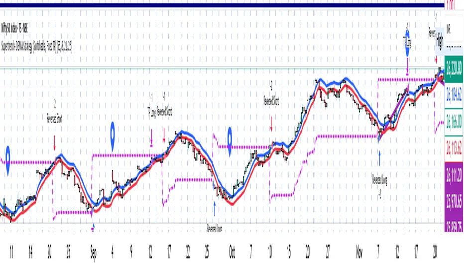
Supertrend + DEMA Strategy ( customised & Switchable, Fixed TP)Supertrend line – a moving line that follows the price and shows whether the market is trending up or down.
If the price goes above this line, it usually means the market is going up.
If the price goes below, it usually means the market is going down.
DEMA (Double Exponential Moving Average) – another line that smooths out price movements to spot trends more clearly.
It calculates an average of prices but reacts faster than a normal moving average.
VWolf – Apex GateOverview
VWolf – Apex Gate is a trend-continuation system that blends a Pivot-weighted Supertrend (PVT ST) with an optional **Normal Supertrend** trigger, all **gated by a 200-EMA directional filter. The strategy’s risk controls are volatility-aware—**stops and targets scale by ATR**, and quantity is computed from a fixed **% risk per trade**. Clear **Backtest / Forwardtest** modes with date windows let you validate on segmented datasets before committing to live use.
Recommended Use
- **Markets:** High-liquidity instruments (indices, large-cap equities, liquid FX and major crypto pairs) where trends and pullbacks are clean.
- **Timeframes:** 15m–1h for active intraday; 4h–1D for swing. Lower timeframes may benefit from stricter EMA gating and slightly wider ATR stops.
- **Workflow:**
1. Start with **Backtest** to set baseline ATR/EMA parameters.
2. Move to **Forwardtest** to confirm generalization.
3. Consider walk-forward or multi-symbol rotation to assess robustness.
Strengths & Precautions
Strengths
- **Dual engine** (PVT ST + Normal ST) improves signal quality; the **EMA gate** screens counter-trend noise.
- **ATR-native** stops/targets standardize risk across regimes/instruments.
- **Capital-proportional sizing** preserves account geometry and smooths drawdowns.
- **Clear test segmentation** supports objective evaluation.
Precautions
- **Whipsaw risk** in tight ranges: widen ATR multipliers, enable the EMA gate, or require co-confirmation.
- **Supertrend-anchored stops** can expand in volatility spikes; ensure **% risk** remains within tolerance.
- **One-position policy** avoids stacking risk but forgoes scaling into strong trends; advanced users may prefer add-on frameworks outside this baseline.
Conclusion
VWolf – Apex Gate seeks to enter shortly after **regime flips**, demanding alignment between a **pivot-aware Supertrend** and (optionally) a **classic Supertrend**, while an **EMA gate** enforces directional discipline. With **ATR-driven** stops/targets and **fixed-fraction** sizing, the system adapts naturally to changing volatility. Use the **Backtest** window to dial ranges and the **Forwardtest** window to prove durability on unseen data. For best results, tailor ATR multipliers and the EMA gate to your instrument’s structure and your personal drawdown tolerance.

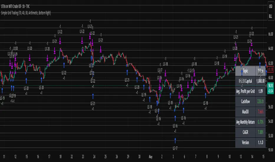
Simple Grid Trading v1.0 [PUCHON]Simple Grid Trading v1.0
Overview
This is a Long-Only Grid Trading Strategy developed in Pine Script v6 for TradingView. It is designed to profit from market volatility by placing a series of Buy Limit orders at predefined price levels. As the price drops, the strategy accumulates positions. As the price rises, it sells these positions at a profit.
Features
Grid Types : Supports both Arithmetic (equal price spacing) and Geometric (equal percentage spacing) grids.
Flexible Order Management : Uses strategy.order for precise control and prevents duplicate orders at the same level.
Performance Dashboard : A real-time table displaying key metrics like Capital, Cashflow, and Drawdown.
Advanced Metrics : Includes Max Drawdown (MaxDD) , Avg Monthly Return , and CAGR calculations.
Customizable : Fully adjustable price range, grid lines, and lot size.
Dashboard Metrics
The dashboard (default: Bottom Right) provides a quick snapshot of the strategy's performance:
Initial Capital : The starting capital defined in the strategy settings.
Lot Size : The fixed quantity of assets purchased per grid level.
Avg. Profit per Grid : The average realized profit for each closed trade.
Cashflow : The total realized net profit (closed trades only).
MaxDD : Maximum Drawdown . The largest percentage drop in equity (realized + unrealized) from a peak.
Avg Monthly Return : The average percentage return generated per month.
CAGR : Compound Annual Growth Rate . The mean annual growth rate of the investment over the specified time period.
Strategy Settings (Inputs)
Grid Settings
Upper Price : The highest price level for the grid.
Lower Price : The lowest price level for the grid.
Number of Grid Lines : The total number of levels (lines) in the grid.
Grid Type :
Arithmetic: Distance between lines is fixed in price terms (e.g., $10, $20, $30).
Geometric: Distance between lines is fixed in percentage terms (e.g., 1%, 2%, 3%).
Lot Size : The fixed amount of the asset to buy at each level.
Dashboard Settings
Show Dashboard : Toggle to hide/show the performance table.
Position : Choose where the dashboard appears on the chart (e.g., Bottom Right, Top Left).
How It Works
Initialization : On the first bar, the script calculates the price levels based on your Upper/Lower price and Grid Type.
Entry Logic :
The strategy places Buy Limit orders at every grid level below the current price.
It checks if a position already exists at a specific level to avoid "stacking" multiple orders on the same line.
Exit Logic :
For every Buy order, a corresponding Sell Limit (Take Profit) order is placed at the next higher grid level.
MaxDD Calculation :
The script continuously tracks the highest equity peak.
It calculates the drawdown on every bar (including intra-bar movements) to ensure accuracy.
Displayed as a percentage (e.g., 5.25%).
Disclaimer
This script is for educational and backtesting purposes only. Grid trading involves significant risk, especially in strong trending markets where the price may move outside your grid range. Always use proper risk management.
Alt Trading: FuturesOne
The FuturesOne Indicator + Strategy will be continuously enhanced to ensure our users receive the most effective and profit-focused trading system at the best possible value. Version 0 (V0) of the FuturesOne Strategy is built on a refined Opening Range Breakout (ORB) framework, augmented with a quantitative regime-detection and filtering layer. This design allows users to tailor their approach: they may opt for consistent daily ORB opportunities or select a mode that applies quantitative filters to surface fewer, but higher-probability, trade setups.

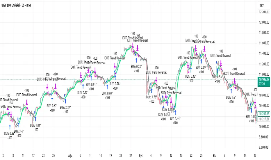
Recursive WMA Angle StrategyDescription: This strategy utilizes a recursive Weighted Moving Average (WMA) calculation to determine the trend direction and strength based on the slope (angle) of the curve. By calculating the angle of the smoothed moving average in degrees, the script filters out noise and aims to enter trades only during strong momentum phases.
How it Works:
Recursive WMA: The script calculates a series of nested WMAs (M1 to M5), creating a very smooth yet responsive curve.
Angle Calculation: It measures the rate of change of this curve over a user-defined lookback period and converts it into an angle (in degrees).
Entry Condition (Long): A long position is opened when the calculated angle exceeds the Min Angle for BUY threshold (default: 0.2), indicating a strong upward trend.
Exit Condition: The position is closed when the angle drops below the Min Angle for SELL threshold (default: -0.2), indicating a sharp trend reversal.
Settings:
MA Settings: Adjust the base lengths for the recursive calculation.
Angle Settings: Fine-tune the sensitivity by changing the Buy/Sell angle thresholds.
Date Filter: Restrict the backtest to a specific date range.
Note: This strategy is designed for Long-Only setups.
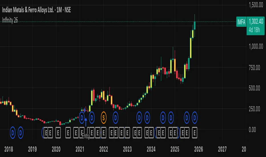
Infinity 26📈 Infinity 26 – Long-Term Investment Signal Indicator
Infinity 26 is a long-term trend-based investment indicator designed to identify high-quality buy and exit points using weekly or monthly candles.
It filters out market noise and focuses only on strong, long-term momentum shifts—making it ideal for wealth creation and slow, steady portfolio growth.
🔹 Key Features
Buy Signals: Automatically highlights strong trend-reversal points where long-term investors can accumulate.
Exit Signals: Shows when the long-term trend weakens, helping protect gains and reduce major drawdowns.
Weekly & Monthly Optimized: Best results when used on 1-week or 1-month timeframe for long-term investing.
Clear Trend Structure: Helps you stay invested during major bull trends and avoid emotional short-term decisions.
Noise-Free: Designed for long-horizon investors—no overtrading, no frequent whipsaws.
🔹 Best For
Long-term investors
Swing-to-position traders
Wealth creation strategies
Portfolio-based investing
🔹 How It Helps You
✔ Avoid wrong entries
✔ Capture major uptrend moves
✔ Reduce risk with timely exits
✔ Build wealth with simple, rule-based signals
CBS Strategy with Trailing Stop _ IK3-Candle High/Low Breakout Strategy – Clean, Powerful, Fully Customizable (Pine Script v6)
A simple yet effective momentum breakout strategy that triggers trades when price closes above the highest high or below the lowest low of the previous 3 completed candles.
Perfect for trending markets (stocks, forex, crypto, indices) on any timeframe.
Key Features:
• Pure price-action breakout logic (no repainting)
• Long & Short entries with visual triangle signals
• Built-in Stop Loss & Take Profit (fixed % or ATR-based)
• Optional Trailing Stop (percentage or ATR multiplier)
• All risk parameters fully adjustable from the settings panel
• Clean on-chart visualization of SL, TP, and active trailing stop levels
• Works on all instruments and timeframes
Default Settings (2:1 Reward/Risk):
• Stop Loss: 1.5%
• Take Profit: 3.0%
• Trailing Stop: 1.0% (optional)
How to Use:
1. Add to chart
2. Adjust risk settings to match your style (fixed % or ATR)
3. Enable/disable trailing stop as needed
4. Backtest and optimize per instrument/timeframe
Fully open-source • No external libraries • Pine Script v6
Great for swing trading, intraday breakouts, or as a base for further enhancements.
Happy trading!

Seawolf Pivot Hunter [Strategy]Overview
Seawolf Pivot Hunter is a practical trading strategy that enhances the classic pivot-box breakout system with a structured risk-management framework. Using ATR-based stop loss and take-profit calculations, position sizing, multi-layer filtering, and daily loss-limit protection, it provides a stable and sustainable trading environment. It preserves the strengths of the original version while adding systems designed to manage real-market risks more effectively.
Core Philosophy
The most important element in trading is not generating profits but controlling losses. Even the best entry signals cannot compensate for a single large loss that wipes out accumulated gains. This strategy precisely calculates the risk exposure for every trade and includes multiple layers of protection to safeguard the account under worst-case scenarios.
Indicator Setup Link
kr.tradingview.com
Example of Optimal Parameter Settings
Asset (Exchange): ETH/USDT (Binance)
Timeframe: 15-minute chart
Pivot Detection Length: 5
Upper Box Width: 2
Lower Box Width: 2
Enable Risk Management: False
Use Trailing Stop: False
Use Volume Filter
-Min Buy Volume % for Long: 50
-Min Sell Volume % for Short: 50
Use Trend Filter (EMA): False
Enable Max Loss Protection
-Max Daily Loss ($): 200
-Max Trades Per Day: 10
Calculated Bars: 50,000
Risk-Management System
Every trade automatically receives a stop-loss level at the moment of entry. The stop is calculated using ATR, adjusting dynamically to market volatility. When volatility increases, the stop widens; in stable conditions, it tightens to reduce unnecessary exits. The default distance is set to twice the ATR.
The standard take-profit level is set to four times the ATR, providing a 1:2 risk-reward structure. With this ratio, even a 50 percent win rate can produce profitability—while the typical trade structure aims for small losses and larger gains to support long-term performance.
A trailing-stop option is also available. Once the trade moves into profit, the stop level automatically trails behind price action, protecting gains while allowing the position to expand when momentum continues.
Position size is calculated automatically based on the selected risk percentage. For example, with a 2 percent risk setting, each stop-loss hit would result in exactly 2 percent of the account balance being lost. This ensures a consistent risk profile regardless of account size.
The daily loss-limit function prevents excessive drawdown by halting new trades once a predefined loss threshold is reached. This helps avoid emotional decision-making after consecutive losses.
A daily trade-limit feature is included as well. The default is 10 trades per day, protecting traders from overtrading and unnecessary fees.
Filtering System
The volume filter analyzes buying and selling pressure within the pivot box. Long trades are allowed only when buy volume exceeds a specified percentage; shorts require sell-volume dominance. The default threshold is 55 percent.
The trend filter uses an EMA to determine market direction. When price is above the 200-EMA, only long signals are permitted; when below, only shorts are allowed. This ensures alignment with the broader trend and reduces counter-trend risk.
Each filter can be toggled independently. More filters generally reduce trade frequency but improve signal quality.
Real-Time Monitoring
A real-time statistics panel displays daily profit/loss, the number of trades taken, the maximum allowed trades, and whether new trades are currently permitted. When daily limits are reached, the panel provides clear visual warnings.
Entry Logic
A trade is validated only after a pivot-box breakout occurs and all active filters—volume, trend, daily loss limit, and daily trade limit—are satisfied. Position size, stop loss, and take-profit levels are then calculated automatically. Entry arrows and labels on the chart help with later review and analysis.
Setup Guide
Risk percentage is the most critical setting. Beginners should start at 1 percent. Anything above 3 percent becomes aggressive.
ATR stop-loss multipliers should reflect asset volatility.
ATR take-profit multipliers determine reward ratio; 4.0 is the standard.
Volume thresholds are typically set between 50–60 percent depending on market conditions.
Daily loss limits are typically 2–5 percent of the account.
Trading Strategy
This strategy performs best in trending environments and works especially well on the 4-hour and daily charts. New users should begin with all filters enabled and trade conservatively. A minimum of one month of paper trading is recommended before committing real capital.
Suitable Users
The strategy is ideal for beginners who lack risk-management experience as well as advanced traders seeking a customizable structure. It is particularly helpful for traders who struggle with emotional decision-making, as pre-defined limits and rules enforce discipline.
Backtesting Guide
Use at least 2–3 years of historical data that includes bullish, bearish, and sideways conditions.
Target metrics:
Sharpe ratio: 1.5 or higher
Maximum drawdown: below 25 percent
Win rate: 40 percent or higher
Total trades: at least 100 for statistical relevance
Optimization Precautions
Avoid over-fitting parameters. Always test values around the “best” setting to verify stability.
Out-of-sample testing is essential for confirming robustness.
Test across multiple assets and timeframes to ensure consistency.
Live Deployment Roadmap
After successful backtesting, follow a gradual rollout:
Paper trading for at least one month
Small-account live testing
Slow scaling as performance stabilizes
Continuous Improvement
Keep a detailed trading journal and evaluate performance each quarter using recent data.
Adapt settings as market conditions evolve.
Conclusion
Seawolf Pivot Hunter aims to provide more than simple trade signals—it is designed to create a stable and sustainable trading system built on disciplined risk management. No strategy is perfect, and long-term success depends on consistency, patience, and strict adherence to rules. Start small, verify results, and scale progressively.
Disclaimer
This strategy is for educational and research purposes only. Past performance does not guarantee future results. All trading decisions are the responsibility of the user.
개요
Seawolf Pivot Hunter는 기본 피봇 박스 브레이크아웃 전략에 전문적인 리스크 관리 시스템을 더한 실전형 트레이딩 전략입니다. ATR 기반의 손절매와 목표가 설정, 포지션 사이징, 다층 필터링 시스템, 일일 손실 제한 기능을 통해 안정적이고 지속 가능한 트레이딩 환경을 제공합니다. 기본 버전의 장점은 유지하면서 실제 시장에서 발생할 수 있는 위험을 체계적으로 관리할 수 있도록 설계되었습니다.
핵심 철학
트레이딩에서 가장 중요한 것은 수익이 아니라 손실 관리입니다. 아무리 훌륭한 진입 조건이 있어도 한 번의 큰 손실로 모든 수익이 사라질 수 있습니다. 이 전략은 각 거래마다 감수할 리스크를 명확히 계산하고, 최악의 상황에서도 계좌를 보호하기 위한 다양한 안전장치를 제공합니다.
지표 적용 링크 공유
kr.tradingview.com
최적 조건값 설정(예시)
"종목(거래소): ETH/USDT(Binance)", "15 분봉 기준"
-Pivot Detection Length: 5
-Upper Box width: 2
-Lower Box width: 2
-Enable Risk Management: False
-Use Trailing Stop: False
-Use Volume Filter
-Min Buy Volume % for Long: 50
-Min Buy Volume % for Long: 50
-Use Trend Filter(EMA): False
-Enable Max Loss Protection
-Max Daily Loss($): 200
-Max Trades Per Day: 10
-Calucated bars: 50000
리스크 관리 시스템
모든 거래는 진입과 동시에 손절매 주문이 자동 설정됩니다. 손절가는 ATR을 기준으로 계산되며, 시장의 변동성에 따라 자동으로 조정됩니다. 변동성이 큰 시장에서는 넓은 손절폭을, 안정적인 시장에서는 좁은 손절폭을 사용해 불필요한 청산을 줄입니다. 기본값은 ATR의 2배입니다.
목표가는 ATR의 4배를 기본값으로 설정하여 손익비 1:2 구조를 유지합니다. 승률이 50퍼센트만 되어도 수익성이 가능하며, 실제로는 손절은 짧고 이익은 길게 가져가는 방식으로 장기 성과를 확보합니다.
트레일링 스톱 기능도 제공됩니다. 포지션이 수익 구간에 들어서면 손절가가 자동으로 함께 움직이며 수익을 보호합니다. 이 기능은 사용자가 켜거나 끌 수 있습니다.
포지션 크기는 리스크 퍼센트 기반으로 자동 계산됩니다. 예를 들어 리스크를 2퍼센트로 설정하면 손절 시 계좌 자산의 2퍼센트만 잃도록 수량이 조절됩니다. 계좌 크기와 무관하게 항상 일정한 비율의 리스크만 감수하게 되는 방식입니다.
일일 손실 제한 기능은 하루에 허용 가능한 최대 손실을 초과하지 않도록 합니다. 지정 금액에 도달하면 당일 거래는 더 이상 실행되지 않습니다. 감정적 거래를 막고 일정한 규율을 유지하도록 돕습니다.
일일 거래 횟수 제한 기능도 제공됩니다. 기본값은 하루 10회로, 과매매와 수수료 증가를 방지합니다.
필터링 시스템
볼륨 필터는 박스 구간 내 매수·매도 압력을 분석해 진입 신호를 검증합니다. 롱은 매수 볼륨이 일정 비율 이상일 때, 숏은 매도 볼륨이 우세할 때만 진입합니다. 기본값은 55퍼센트입니다.
추세 필터는 EMA를 사용하며, 가격이 200EMA 위에 있을 때는 롱 신호만, 아래에서는 숏 신호만 허용합니다. 큰 추세 방향에만 거래하여 역추세 리스크를 줄입니다.
필터는 독립적으로 켜고 끌 수 있으며, 필터가 많을수록 거래 횟수는 줄지만 신호 품질은 향상됩니다.
실시간 모니터링
화면에 실시간 통계 테이블이 표시되며, 일일 손익, 거래 횟수, 최대 허용 횟수, 현재 거래 가능 여부가 즉시 확인됩니다. 손실 제한 또는 거래 제한 도달 시 시각적으로 표시됩니다.
진입 로직
피봇 박스 브레이크아웃 발생 후 볼륨 필터, 추세 필터, 일일 손실·거래 제한을 모두 통과하면 포지션 크기를 계산하고 손절·목표가를 설정한 뒤 진입합니다. 진입 지점에는 화살표와 레이블이 표시되어 분석에 도움을 줍니다.
설정 가이드
리스크 퍼센트는 가장 중요한 설정입니다. 초보자는 1퍼센트를 추천하며 3퍼센트 이상은 위험합니다.
손절 ATR 배수는 자산 특성에 맞게 조절합니다.
목표가 ATR 배수는 손익비를 결정하며 기본값은 4.0입니다.
볼륨 비율은 시장 상황에 따라 50~60퍼센트 내외로 조정합니다.
일일 손실 제한은 계좌의 2~5퍼센트 수준이 적절합니다.
사용 전략
추세가 명확한 시장에서 가장 효과적이며, 4시간봉 또는 일봉을 추천합니다. 초반에는 모든 필터를 켜고 보수적으로 시작하며, 최소 한 달간 페이퍼 트레이딩을 권장합니다.
적합한 사용자
리스크 관리 경험이 부족한 초보자부터, 커스터마이징을 원하는 경험자까지 폭넓게 적합합니다. 감정적 트레이딩을 억제하는 기능이 있어 규율 유지가 어렵던 트레이더에게 특히 유용합니다.
백테스트 가이드
최소 2~3년 데이터로 테스트하며, 상승·하락·횡보 모두 포함해야 합니다.
샤프비율 1.5 이상, 최대 낙폭 25퍼센트 이하를 목표로 합니다.
승률은 40퍼센트 이상이면 충분합니다.
최소 100회 이상 거래가 있어야 통계적으로 의미가 있습니다.
최적화 주의사항
과최적화를 피하고 주변 값도 테스트해야 합니다.
샘플 외 기간 검증은 필수입니다.
여러 자산·여러 시간대에서 테스트하여 일관성을 확인해야 합니다.
실전 적용 로드맵
백테스트 후 바로 실전 투입하지 말고, 한 달 이상의 페이퍼 트레이딩 → 소액 실전 → 점진적 확대 순으로 진행합니다.
지속적 개선
일지를 기록하고 분기마다 최신 데이터로 점검합니다.
시장 변화에 따라 유연하게 조정해야 합니다.
마치며
Seawolf Pivot Hunter는 단순 신호 제공을 넘어, 안전하고 지속 가능한 트레이딩 환경 구축을 목표로 합니다. 어떤 전략도 완벽할 수 없으며, 장기적 성공을 위해서는 규칙 준수와 인내가 가장 중요합니다. 충분한 검증을 거쳐 작은 금액으로 시작하고 점진적으로 확장해나가는 접근을 추천합니다.
면책 조항
이 전략은 교육 및 연구 목적이며, 과거 성과는 미래를 보장하지 않습니다. 모든 투자 결정은 본인의 판단과 책임 하에 이루어져야 합니다.

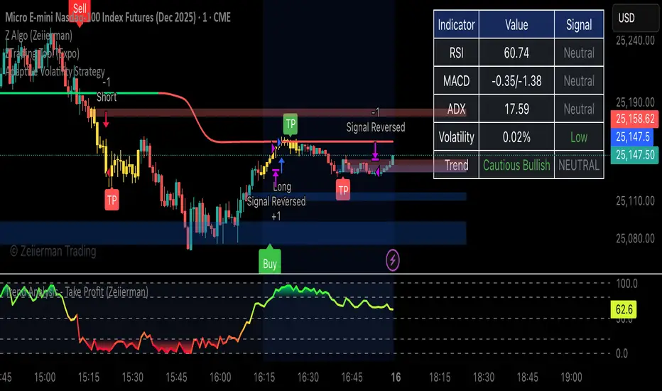
Adaptive Volatility StrategyHere's a professional description for publishing your indicator:
Adaptive Volatility Strategy - Multi-Indicator Confirmation System
A comprehensive trading strategy that combines multiple technical indicators with adaptive volatility filtering to identify high-probability trade setups while managing risk effectively.
Key Features:
Multi-Indicator Confirmation: Combines RSI, MACD, and ADX signals with trend analysis (20/50/200 EMAs) to reduce false signals and improve entry quality
Adaptive Volatility Filter: Intelligent volatility detection using ATR that can filter trades based on either fixed percentage thresholds or multiples of average volatility, helping avoid unstable market conditions
Flexible Session Filtering: Optional time-based trading windows with customizable hours and trading days to align with your preferred market sessions
Smart Signal Generation: Requires minimum signal confirmations before entering trades, with separate tracking for directional and confirmation signals
Comprehensive Risk Management: Configurable take profit and stop loss percentages with automatic position exits on signal reversals
Real-Time Dashboard: Visual display showing current indicator values, signals, volatility levels, and trend direction for quick market assessment
Strategy Logic:
Enters long when bullish signals outnumber bearish signals (minimum 2 signals) with ADX confirmation
Enters short when bearish signals outnumber bullish signals with ADX confirmation
All trades must pass volatility and session filters when enabled
Exits on take profit, stop loss, or signal reversal
Best Used For:
Swing trading on 1H to daily timeframes
Markets with clear trending behavior
Traders who prefer multiple confirmations before entering positions
Note: This is a complete strategy with entry/exit logic. Backtest thoroughly and adjust parameters for your specific instrument and timeframe before live trading.
WDO DayTrade Brasil - by IchilinhaWDO DayTrade Brazil - Advanced Strategy with Risk Control
Overview
A complete day trading strategy developed specifically for trading Mini Dollar (WDO) futures in the Brazilian market (B3). It combines multi-timeframe technical analysis, trend/sideway filters, advanced risk management with ATR, and strict controls on the time and number of daily trades.

WIN DayTrade Brasil - by Ichilinha
A comprehensive day trading strategy developed specifically for trading the Mini Index (WIN) on the Brazilian market (B3). It combines multi-timeframe technical analysis, trend/sideway filters, advanced risk management with ATR, and strict controls on the time and number of daily trades.
Note: Always trade responsibly. Day trading requires technical knowledge, emotional discipline, and proper risk management. Never trade with money you cannot afford to lose.

Morning Straddle Backtest + Range Filter Morning Straddle Backtest
Purpose:
This script tests a Morning Straddle concept where a trader enters both long and short breakout orders based on the overnight range (22:00–06:00 by default).
It is designed for backtesting the effectiveness of volatility breakouts following low-volume overnight sessions.
Setup
Overnight session: 22:00–06:00 (adjustable).
At the end of the overnight session, the script automatically places:
A long stop order above the range high.
A short stop order below the range low.
Both use an ATR-based buffer for cleaner breakouts (default 5%).
When one side triggers, the opposite order is cancelled if OCO mode is active.
Adjustable Parameters
- Session - Defines the overnight hours used for the range.
- ATR Length - Number of bars used for ATR calculation.
- ATR Buffer % - Distance above/below range for entry & stop placement.
- Risk:Reward Ratio - Determines the TP distance relative to SL.
- Stop-Loss - Choose between “Behind Range” or “Mid-Range (50%)” with ATR buffer added.
- OCO - Cancels opposite order once one side triggers.
- Close All EOD - Closes all open trades at the end of day (default 22:00).
- Range Filter – Enables filtering of trades only when the overnight range size falls within a defined threshold.
-Min Range / Max Range – Define acceptable range size boundaries.
-Display Units – Select whether the filter is measured in Price Change, Pips, or Points.
- Stats Panel Settings – Toggle visibility, position (Top/Bottom Left/Right), and background opacity.
Visual
The overnight range (22:00–06:00) is highlighted on the chart with a teal background for clarity.
No lines are drawn for the high and low.
Strategy Notes
Works best on 5m or 15m charts where the overnight range can be clearly defined.
Backtests should be run over multiple months to gauge performance consistency.
Can be adapted for other markets by adjusting session times and ATR settings. For example, S&P initial balance breakout using 14:30-15:30 range time.
Stats Panel Displays
- 20-Day Range Data: Maximum, Average, and Minimum range sizes.
- Today’s Range: With automatic classification — Huge, Normal, or Small.
- Average Winning Range: Average size of the overnight range on profitable days.
- Average Losing Range: Average size of the overnight range on losing days.
- Filter Status: Displays whether the range met the filter criteria — Range OK, Skipped, or Off.

AlgoIndexOS-ES-FuturesAlgoIndexOS — ES Futures Strategy v2.0 (5-Minute RTH)
Scope (read first)
ES on 5-minute only, RTH session. The strategy operates on U.S. Regular Trading Hours (09:30–16:00 ET) using a 5-minute ES chart. It builds an Opening Session Range (OSR) from the RTH open, then runs a breakout engine when internal quality conditions are met. Exits are target-based with an intrabar touch-to-flat safety. Positions are flattened at the RTH session end by default. Alerts can post JSON to your Webhook URL for automation.
What this is
One intraday engine with four curated presets (“Stages”) tuned for distinct segments of the NY session. Stages keep the core logic consistent while applying time-of-day context and conservative governors. Single invite-only listing; not a multi-post suite.
How it trades (high-level)
Range context: Builds and locks the OSR from the opening bell; entries only arm after the range is set.
Quality gating: Trades only when internal trend/volatility/confirmation conditions align (no parameter disclosure).
Breakout execution: Signals at bar close; bracket exits manage take-profit (limit) with an intrabar “TP-touch” safety to avoid phantom fills; optional stop-loss.
Session safety: Positions flat at RTH close by default (time exit).
(No settings or thresholds are disclosed; presets encapsulate research choices.)
Stages (session templates; one engine)
A single Stage selector chooses among four presets optimized for different parts of the RTH session (morning vs mid-day; long/short focus). Internal parameters remain fixed to preserve tested behavior.
Public inputs (kept minimal)
Stage (choose your preset)
TP / SL (points) shown for transparency; effective values are governed by the selected preset to maintain consistency with research.
Optional display overlays (status line/markers) for readability.
Alerts (how to use)
Create an alert on the strategy and choose Strategy → Order fills. Use a webhook if you want automation. The payload includes the exact chart symbol so it works on ES1! or a specific ES contract:
{
"tv_symbol": "{{ticker}}",
"tv_exchange": "{{exchange}}",
"action": "buy|sell|exit",
"price": {{close}},
"time": "{{timenow}}"
}
If your receiver needs a fixed root (e.g., “ES”), map it on your server using tv_symbol for context.
Backtest & assumptions
Backtest assumptions (initial capital, commission, slippage, margin) are user-configurable in TradingView. Results on your chart reflect your settings. This script evaluates ES fills on 5-minute RTH bars; live execution will differ.
Operating notes
Use on ES only, 5-minute timeframe, RTH session.
If you run multiple Stages, use separate charts/tabs and coordinate net exposure in your own tooling if needed.
Publish with a clean chart for clarity.
Disclosures (compliance)
No investment advice. This script is for research/education and tooling only. It does not provide investment, legal, tax, or accounting advice and does not recommend any security, instrument, or strategy. Use at your own risk.
Hypothetical performance (CFTC 4.41). Hypothetical or simulated results have many limitations, and no representation is made that any account will achieve similar outcomes. Past performance is not necessarily indicative of future results.
Futures risk. Trading futures involves substantial risk of loss and is not suitable for all investors. Leverage, gaps, slippage, and connectivity can cause losses exceeding initial investment.
Backtesting limitations. Results depend on data quality, chart resolution, session filters, and user assumptions; live execution will differ.
Intellectual property. © 2025 AlgoIndex. All Rights Reserved. Redistribution, resale, or decompilation prohibited without written consent.

12M SMA Timing (HTF-safe, 100% equity)Buy when S&P500 closes above 12M moving average. Sell when it closes below it. Monthly only.

WIN1! • Crossing EMAs• (By Mesquita, v7)Moving average crossover strategy for intraday movements, especially in the continuous index (WIN1!) on the Brazilian stock exchange B³. The strategy is customizable for time windows, has a filter for trades only above the long-term average, whether only long, only short, or both, with or without stop loss.

KZ One — Scalping Training StrategyKZ One is a scalping strategy developed for M1 and M5 timeframes. It is designed to help traders study and practice short-term market behavior by using structured zones to highlight potential entry and exit areas. The strategy allows customization of Risk (USD) and Take Profit (R multiple) parameters for flexible trade management. Additional tools include ATR-based filters to skip low-volatility conditions and a Pre-Alert Lead (bars) option that notifies users ahead of possible setups. KZ One is intended for educational and analytical purposes, promoting disciplined and consistent trading practice.

💸 DCA Accumulation Strategy (USD‑Based Scaling)Buy when blue arrow appears, if the next arrow is lower than the last increase your position. This will pull your average cost down slowly over time.
