[GYTS] Volatility Toolkit Volatility Toolkit
🌸 Part of GoemonYae Trading System (GYTS) 🌸
🌸 --------- INTRODUCTION --------- 🌸
💮 What is Volatility Toolkit?
Volatility Toolkit is a comprehensive volatility analysis indicator featuring academically-grounded range-based estimators. Unlike simplistic measures like ATR, these estimators extract maximum information from OHLC data — resulting in estimates that are 5-14× more statistically efficient than traditional close-to-close methods.
The indicator provides two configurable estimator slots, weighted aggregation, adaptive threshold detection, and regime identification — all with flexible smoothing options via
GYTS FiltersToolkit integration.
💮 Why Use This Indicator?
Standard volatility measures (like simple standard deviation) are highly inefficient, requiring large amounts of data to produce stable estimates. Academic research has shown that range-based estimators extract far more information from the same price data:
• Statistical Efficiency — Yang-Zhang achieves up to 14× the efficiency of close-to-close variance, meaning you can achieve the same estimation accuracy with far fewer bars
• Drift Independence — Rogers-Satchell and Yang-Zhang correctly isolate variance even in strongly trending markets where simpler estimators become biased
• Gap Handling — Yang-Zhang properly accounts for overnight gaps, critical for equity markets
• Regime Detection — Built-in threshold modes identify when volatility enters elevated or suppressed states
↑ Overview showing Yang-Zhang volatility with dynamic threshold bands and regime background colouring
🌸 --------- HOW IT WORKS --------- 🌸
💮 Core Concept
The toolkit groups volatility estimators by their output scale to ensure valid comparisons and aggregations:
• Log-Return Scale (σ) — Close-to-Close, Parkinson, Garman-Klass, Rogers-Satchell, Yang-Zhang. These are comparable and can be aggregated. Annualisable via √(periods_per_year) scaling.
• Price Unit Scale ($) — ATR. Measures volatility in absolute price terms, directly usable for stop-loss placement.
• Percentage Scale (%) — Chaikin Volatility. Measures the rate of change of the trading range — whether volatility is expanding or contracting.
Only estimators with the same scale can be meaningfully compared or aggregated. The indicator enforces this and warns when mixing incompatible scales.
💮 Range-Based Estimator Overview
Range-based estimators utilise High, Low, Open, and Close prices to extract significantly more information about the underlying diffusion process than close-only methods:
• Parkinson (1980) — Uses High-Low range. ~5× more efficient than close-to-close. Assumes zero drift.
• Garman-Klass (1980) — Incorporates Open and Close. ~7.4× more efficient. Assumes zero drift, no gaps.
• Rogers-Satchell (1991) — Drift-independent. Superior in trending markets where Parkinson/GK become biased.
• Yang-Zhang (2000) — Composite estimator handling both drift and overnight gaps. Up to 14× more efficient.
💮 Theoretical Background
• Parkinson, M. (1980). The Extreme Value Method for Estimating the Variance of the Rate of Return. Journal of Business, 53 (1), 61–65. DOI
• Garman, M.B. & Klass, M.J. (1980). On the Estimation of Security Price Volatilities from Historical Data. Journal of Business, 53 (1), 67–78. DOI
• Rogers, L.C.G. & Satchell, S.E. (1991). Estimating Variance from High, Low and Closing Prices. Annals of Applied Probability, 1 (4), 504–512. DOI
• Yang, D. & Zhang, Q. (2000). Drift-Independent Volatility Estimation Based on High, Low, Open, and Close Prices. Journal of Business, 73 (3), 477–491. DOI
🌸 --------- KEY FEATURES --------- 🌸
💮 Feature Reference
Estimators (8 options across 3 scale groups):
• Close-to-Close — Classical benchmark using closing prices only. Least efficient but useful as baseline. Log-return scale.
• Parkinson — Range-based (High-Low), ~5× more efficient than close-to-close. Assumes zero drift. Log-return scale.
• Garman-Klass — OHLC-optimised, ~7.4× more efficient. Assumes zero drift, no gaps. Log-return scale.
• Rogers-Satchell — Drift-independent, handles trending markets where Parkinson/GK become biased. Log-return scale.
• Yang-Zhang — Gap-aware composite, most comprehensive (up to 14× efficient). Uses internal rolling variance (unsmoothed). Log-return scale.
• Std Dev — Standard deviation of log returns. Log-return scale.
• ATR — Average True Range in absolute price units. Useful for stop-loss placement. Price unit scale.
• Chaikin — Rate of change of range. Measures volatility expansion/contraction, not level. Percentage scale.
Smoothing Filters (10 options via FiltersToolkit):
• SMA / EMA — Classical moving averages
• Super Smoother (2-Pole / 3-Pole) — Ehlers IIR filter with excellent noise reduction
• Ultimate Smoother (2-Pole / 3-Pole) — Near-zero lag in passband
• BiQuad — Second-order IIR with configurable Q factor
• ADXvma — Adaptive smoothing, flat during ranging periods
• MAMA — MESA Adaptive Moving Average (cycle-adaptive)
• A2RMA — Adaptive Autonomous Recursive MA
Threshold Modes:
• Static — Fixed threshold values you define (e.g., 0.025 annualised)
• Dynamic — Adaptive bands: baseline ± (standard deviation × multiplier)
• Percentile — Threshold at Nth percentile of recent history (e.g., 80th percentile for high)
Visual Features:
• Level-based colour gradient — Line colour shifts with percentile rank (warm = high vol, cool = low vol)
• Fill to zero — Gradient fill intensity proportional to volatility level
• Threshold fills — Intensity-scaled fills when thresholds are breached
• Regime background — Chart background indicates HIGH/NORMAL/LOW volatility state
• Legend table — Displays estimator names, parameters, current values with percentile ranks (P##)
💮 Dual Estimator Slots
Compare two volatility estimators side-by-side. Each slot independently configures:
• Estimator type (8 options across three scale groups)
• Lookback period and smoothing filter
• Colour palette and visual style
This enables direct comparison between estimators (e.g., Yang-Zhang vs Rogers-Satchell) or between different parameterisations of the same estimator.
↑ Yang-Zhang (reddish) and Rogers-Satchell (greenish)
💮 Flexible Smoothing via FiltersToolkit
All estimators (except Yang-Zhang, which uses internal rolling variance) support configurable smoothing through 10 filter types. Using Infinite Impulse Response (IIR) filters instead of SMA avoids the "drop-off artefact" where volatility readings crash when old spikes exit the window.
Example: Same estimator (Parkinson) with different smoothing filters
Add two instances of Volatility Toolkit to your chart:
• Instance 1: Parkinson with SMA smoothing (lookback 14)
• Instance 2: Parkinson with Super Smoother 2-Pole (lookback 14)
Notice how SMA creates sharp drops when volatile bars exit the window, while Super Smoother maintains a gradual transition.
↑ Two Parkinson estimators — SMA (red mono-colour, showing drop-off artefacts) vs Super Smoother (turquoise mono colour, with smooth transitions)
↑ Garman-Klass with BiQuad (orangy) and 2-pole SuperSmoother filters (greenish)
💮 Weighted Aggregation
Combine multiple estimators into a single weighted average. The indicator automatically:
• Validates scale compatibility (only same-scale estimators can be aggregated)
• Normalises weights (so 2:1 means 67%:33%)
• Displays clear warnings when scales differ
Example: Robust volatility estimate
Combine Yang-Zhang (handles gaps) with Rogers-Satchell (handles drift) using equal weights:
• E1: Yang-Zhang (14)
• E2: Rogers-Satchell (14)
• Aggregation: Enabled, weights 1:1
The aggregated line (with "fill to zero" enabled) provides a more robust estimate by averaging two complementary methodologies.
↑ Yang-Zhang + Rogers-Satchell with aggregation line (thicker) showing combined estimate (notice how opening gaps are handled differently)
Example: Trend-weighted aggregation
In strongly trending markets, weight Rogers-Satchell more heavily since it's drift-independent:
• Estimator 1: Garman-Klass (faster, higher weight in ranging)
• Estimator 2: Rogers-Satchell (drift-independent, higher weight in trends)
• Aggregation: weights 1:2 (favours RS during trends)
💮 Adaptive Threshold Detection
Three threshold modes for identifying volatility regime shifts. Threshold breaches are visualised with intensity-scaled fills that grow stronger the further volatility exceeds the threshold.
Example: Dynamic thresholds for regime detection
Configure dynamic thresholds to automatically adapt to market conditions:
• High Threshold Mode: Dynamic (baseline + 2× std dev)
• Low Threshold Mode: Dynamic (baseline - 2× std dev)
• Show threshold fills: Enabled
This creates adaptive bands that widen during volatile periods and narrow during calm periods.
Example: Percentile-based thresholds
Use percentile mode for context-aware regime detection:
• High Threshold Mode: Percentile (96th)
• Low Threshold Mode: Percentile (4th)
• Percentile Lookback: 500
This identifies when volatility enters the top/bottom 4% of its recent distribution.
↑ Different threshold settings, where the dynamic and percentile methods show adaptive bands that widen during volatile periods, with fill intensity varying by breach magnitude. Regime detection (see next) is enabled too.
💮 Regime Background Colouring
Optional background colouring indicates the current volatility regime:
• High Volatility — Warm/alert background colour
• Normal — No background (neutral)
• Low Volatility — Cool/calm background colour
Select which source (Estimator 1, Estimator 2, or Aggregation) drives the regime display.
Example: Regime filtering for trade decisions
Use regime background to filter trading signals from other indicators:
• Regime Source: Aggregation
• Background Transparency: 90 (subtle)
When the background shows HIGH volatility (warm), consider tighter stops. When LOW (cool), watch for breakout setups.
↑ Regime background emphasis for breakout strategies. Note the interesting A2RMA smoothing for this case.
🌸 --------- USAGE GUIDE --------- 🌸
💮 Getting Started
1. Add the indicator to your chart
2. Estimator 1 defaults to Yang-Zhang (14) — the most comprehensive estimator for gapped markets
3. Keep "Annualise Volatility" enabled to express values in standard annualised form
4. Observe the legend table for current values and percentile ranks (P##). Hover over the table cells to see a little more info in the tooltip.
💮 Choosing an Estimator
• Trending equities with gaps — Yang-Zhang. Handles both drift and overnight gaps optimally.
• Crypto (24/7 trading) — Rogers-Satchell. Drift-independent without Yang-Zhang's multi-period lag.
• Ranging markets — Garman-Klass or Parkinson. Simpler, no drift adjustment needed.
• Price-based stops — ATR. Output in price units, directly usable for stop distances.
• Regime detection — Combine any estimator with threshold modes enabled.
💮 Interpreting Output
• Value (P##) — The volatility reading with percentile rank. "0.1523 (P75)" means 0.1523 annualised volatility at the 75th percentile of recent history.
• Colour gradient — Warmer colours = higher percentile (elevated volatility), cooler colours = lower percentile.
• Threshold fills — Intensity indicates how far beyond the threshold the current reading is.
• ⚠️ HIGH / 🔻 LOW — Table indicators when thresholds are breached.
🌸 --------- ALERTS --------- 🌸
💮 Direction Change Alerts
• Estimator 1/2 direction change — Triggers when volatility inflects (rising to falling or vice versa)
💮 Cross Alerts
• E1 crossed E2 — Triggers when the two estimator lines cross
💮 Threshold Alerts
• E1/E2/Aggr High Volatility — Triggers when volatility breaches the high threshold
• E1/E2/Aggr Low Volatility — Triggers when volatility falls below the low threshold
💮 Regime Change Alerts
• E1/E2/Aggr Regime Change — Triggers when the volatility regime transitions (High ↔ Normal ↔ Low)
🌸 --------- LIMITATIONS --------- 🌸
• Drift bias in Parkinson/GK — These estimators overestimate variance in trending conditions. Switch to Rogers-Satchell or Yang-Zhang for trending markets.
• Yang-Zhang minimum lookback — Requires at least 2 bars (enforced internally). Cannot produce instantaneous readings like other estimators.
• Flat candles — Single-tick bars produce near-zero variance readings. Use higher timeframes for illiquid assets.
• Discretisation bias — Estimates degrade when ticks-per-bar is very small. Consider higher timeframes for thinly traded instruments.
• Scale mixing — Different scale groups (log-return, price unit, percentage) cannot be meaningfully compared or aggregated. The indicator warns but does not prevent display.
🌸 --------- CREDITS --------- 🌸
💮 Academic Sources
• Parkinson, M. (1980). The Extreme Value Method for Estimating the Variance of the Rate of Return. Journal of Business, 53 (1), 61–65. DOI
• Garman, M.B. & Klass, M.J. (1980). On the Estimation of Security Price Volatilities from Historical Data. Journal of Business, 53 (1), 67–78. DOI
• Rogers, L.C.G. & Satchell, S.E. (1991). Estimating Variance from High, Low and Closing Prices. Annals of Applied Probability, 1 (4), 504–512. DOI
• Yang, D. & Zhang, Q. (2000). Drift-Independent Volatility Estimation Based on High, Low, Open, and Close Prices. Journal of Business, 73 (3), 477–491. DOI
• Wilder, J.W. (1978). New Concepts in Technical Trading Systems . Trend Research.
💮 Libraries Used
• VolatilityToolkit Library — Range-based estimators, smoothing, and aggregation functions
• FiltersToolkit Library — Advanced smoothing filters (Super Smoother, Ultimate Smoother, BiQuad, etc.)
• ColourUtilities Library — Colour palette management and gradient calculations
Goemonyae

[GYTS] VolatilityToolkit LibraryVolatilityToolkit Library
🌸 Part of GoemonYae Trading System (GYTS) 🌸
🌸 --------- INTRODUCTION --------- 🌸
💮 What Does This Library Contain?
VolatilityToolkit provides a comprehensive suite of volatility estimation functions derived from academic research in financial econometrics. Rather than relying on simplistic measures, this library implements range-based estimators that extract maximum information from OHLC data — delivering estimates that are 5–14× more efficient than traditional close-to-close methods.
The library spans the full volatility workflow: estimation, smoothing, and regime detection.
💮 Key Categories
• Range-Based Estimators — Parkinson, Garman-Klass, Rogers-Satchell, Yang-Zhang (academically-grounded variance estimators)
• Classical Measures — Close-to-Close, ATR, Chaikin Volatility (baseline and price-unit measures)
• Smoothing & Post-Processing — Asymmetric EWMA for differential decay rates
• Aggregation & Regime Detection — Multi-horizon blending, MTF aggregation, Volatility Burst Ratio
💮 Originality
To the best of our knowledge, no other TradingView script combines range-based estimators (Parkinson, Garman-Klass, Rogers-Satchell, Yang-Zhang), classical measures, and regime detection tools in a single package. Unlike typical volatility implementations that offer only a single method, this library:
• Implements four academically-grounded range-based estimators with proper mathematical foundations
• Handles drift bias and overnight gaps, issues that plague simpler estimators in trending markets
• Integrates with GYTS FiltersToolkit for advanced smoothing (10 filter types vs. typical SMA-only)
• Provides regime detection tools (Burst Ratio, MTF aggregation) for systematic strategy integration
• Standardises output units for seamless estimator comparison and swapping
🌸 --------- ADDED VALUE --------- 🌸
💮 Academic Rigour
Each estimator implements peer-reviewed methodologies with proper mathematical foundations. The library handles aspects that are easily missed, e.g. drift independence, overnight gap adjustment, and optimal weighting factors. All functions include guards against edge cases (division by zero, negative variance floors, warmup handling).
💮 Statistical Efficiency
Range-based estimators extract more information from the same data. Yang-Zhang achieves up to 14× the efficiency of close-to-close variance, meaning you can achieve the same estimation accuracy with far fewer bars — critical for adapting quickly to changing market conditions.
💮 Flexible Smoothing
All estimators support configurable smoothing via the GYTS FiltersToolkit integration. Choose from 10 filter types to balance responsiveness against noise reduction:
• Ultimate Smoother (2-Pole / 3-Pole) — Near-zero lag; the 3-pole variant is a GYTS design with tunable overshoot
• Super Smoother (2-Pole / 3-Pole) — Excellent noise reduction with minimal lag
• BiQuad — Second-order IIR filter with quality factor control
• ADXvma — Adaptive smoothing based on directional volatility
• MAMA — Cycle-adaptive moving average
• A2RMA — Adaptive autonomous recursive moving average
• SMA / EMA — Classical averages (SMA is default for most estimators)
Using Infinite Impulse Response (IIR) filters (e.g. Super Smoother, Ultimate Smoother) instead of SMA avoids the "drop-off artefact" where volatility readings crash when old spikes exit the window.
💮 Plug-and-Play Integration
Standardised output units (per-bar log-return volatility) make it trivial to swap estimators. The annualize() helper converts to yearly volatility with a single call. All functions work seamlessly with other GYTS components.
🌸 --------- RANGE-BASED ESTIMATORS --------- 🌸
These estimators utilise High, Low, Open, and Close prices to extract significantly more information about the underlying diffusion process than close-only methods.
💮 parkinson()
The Extreme Value Method -- approximately 5× more efficient than close-to-close, requiring about 80% less data for equivalent accuracy. Uses only the High-Low range, making it simple and robust.
• Assumption: Zero drift (random walk). May be biased in strongly trending markets.
• Best for: Quick volatility reads when drift is minimal.
• Parameters: smoothing_length (default 14), filter_type (default SMA), smoothing_factor (default 0.7)
Source: Parkinson, M. (1980). The Extreme Value Method for Estimating the Variance of the Rate of Return. Journal of Business, 53 (1), 61–65. DOI
💮 garman_klass()
Extends Parkinson by incorporating Open and Close prices, achieving approximately 7.4× efficiency over close-to-close. Implements the "practical" analytic estimator (σ̂²₅) which avoids cross-product terms whilst maintaining near-optimal efficiency.
• Assumption: Zero drift, continuous trading (no gaps).
• Best for: Markets with minimal overnight gaps and ranging conditions.
• Parameters: smoothing_length (default 14), filter_type (default SMA), smoothing_factor (default 0.7)
Source: Garman, M.B. & Klass, M.J. (1980). On the Estimation of Security Price Volatilities from Historical Data. Journal of Business, 53 (1), 67–78. DOI
💮 rogers_satchell()
The drift-independent estimator correctly isolates variance even in strongly trending markets where Parkinson and Garman-Klass become significantly biased. Uses the formula: ln(H/C)·ln(H/O) + ln(L/C)·ln(L/O).
• Key advantage: Unbiased regardless of trend direction or magnitude.
• Best for: Trending markets, crypto (24/7 trading with minimal gaps), general-purpose use.
• Parameters: smoothing_length (default 14), filter_type (default SMA), smoothing_factor (default 0.7)
Source: Rogers, L.C.G. & Satchell, S.E. (1991). Estimating Variance from High, Low and Closing Prices. Annals of Applied Probability, 1 (4), 504–512. DOI
💮 yang_zhang()
The minimum-variance composite estimator — both drift-independent AND gap-aware. Combines overnight returns, open-to-close returns, and the Rogers-Satchell component with optimal weighting to minimise estimator variance. Up to 14× more efficient than close-to-close.
• Parameters: lookback (default 14, minimum 2), alpha (default 1.34, optimised for equities).
• Best for: Equity markets with significant overnight gaps, highest-quality volatility estimation.
• Note: Unlike other estimators, Yang-Zhang does not support custom filter types — it uses rolling sample variance internally.
Source: Yang, D. & Zhang, Q. (2000). Drift-Independent Volatility Estimation Based on High, Low, Open, and Close Prices. Journal of Business, 73 (3), 477–491. DOI
🌸 --------- CLASSICAL MEASURES --------- 🌸
💮 close_to_close()
Classical sample variance of logarithmic returns. Provided primarily as a baseline benchmark — it is approximately 5–8× less efficient than range-based estimators, requiring proportionally more data for the same accuracy.
• Parameters: lookback (default 14), filter_type (default SMA), smoothing_factor (default 0.7)
• Use case: Comparison baseline, situations requiring strict methodological consistency with academic literature.
💮 atr()
Average True Range -- measures volatility in price units rather than log-returns. Directly interpretable for stop-loss placement (e.g., "2× ATR trailing stop") and handles gaps naturally via the True Range formula.
• Output: Price units (not comparable across different price levels).
• Parameters: smoothing_length (default 14), filter_type (default SMA), smoothing_factor (default 0.7)
• Best for: Position sizing, trailing stops, any application requiring volatility in currency terms.
Source: Wilder, J.W. (1978). New Concepts in Technical Trading Systems . Trend Research.
💮 chaikin_volatility()
Rate of Change of the smoothed trading range. Unlike level-based measures, Chaikin Volatility shows whether volatility is expanding or contracting relative to recent history.
• Output: Percentage change (oscillates around zero).
• Parameters: length (default 10), roc_length (default 10), filter_type (default EMA), smoothing_factor (default 0.7)
• Interpretation: High values suggest nervous, wide-ranging markets; low values indicate compression.
• Best for: Detecting volatility regime shifts, breakout anticipation.
🌸 --------- SMOOTHING & POST-PROCESSING --------- 🌸
💮 asymmetric_ewma()
Differential smoothing with separate alphas for rising versus falling volatility. Allows volatility to spike quickly (fast reaction to shocks) whilst decaying slowly (stability). Essential for trailing stops that should widen rapidly during turbulence but narrow gradually.
• Parameters: alpha_up (default 0.1), alpha_down (default 0.02).
• Note: Stateful function — call exactly once per bar.
💮 annualize()
Converts per-bar volatility to annualised volatility using the square-root-of-time rule: σ_annual = σ_bar × √(periods_per_year).
• Parameters: vol (series float), periods (default 252 for daily equity bars).
• Common values: 365 (crypto), 52 (weekly), 12 (monthly).
🌸 --------- AGGREGATION & REGIME DETECTION --------- 🌸
💮 weighted_horizon_volatility()
Blends volatility readings across short, medium, and long lookback horizons. Inspired by the Heterogeneous Autoregressive (HAR-RV) model's recognition that market participants operate on different time scales.
• Default horizons: 1-bar (short), 5-bar (medium), 22-bar (long).
• Default weights: 0.5, 0.3, 0.2.
• Note: This is a weighted trailing average, not a forecasting regression. For true HAR-RV forecasting, it would be required to fit regression coefficients.
Inspired by: Corsi, F. (2009). A Simple Approximate Long-Memory Model of Realized Volatility. Journal of Financial Econometrics .
💮 volatility_mtf()
Multi-timeframe aggregation for intraday charts. Combines base volatility with higher-timeframe (Daily, Weekly, Monthly) readings, automatically scaling HTF volatilities down to the current timeframe's magnitude using the square-root-of-time rule.
• Usage: Calculate HTF volatilities via request.security() externally, then pass to this function.
• Behaviour: Returns base volatility unchanged on Daily+ timeframes (MTF aggregation not applicable).
💮 volatility_burst_ratio()
Regime shift detector comparing short-term to long-term volatility.
• Parameters: short_period (default 8), long_period (default 50), filter_type (default Super Smoother 2-Pole), smoothing_factor (default 0.7)
• Interpretation: Ratio > 1.0 indicates expanding volatility; values > 1.5 often precede or accompany explosive breakouts.
• Best for: Filtering entries (e.g., "only enter if volatility is expanding"), dynamic risk adjustment, breakout confirmation.
🌸 --------- PRACTICAL USAGE NOTES --------- 🌸
💮 Choosing an Estimator
• Trending equities with gaps: yang_zhang() — handles both drift and overnight gaps optimally.
• Crypto (24/7 trading): rogers_satchell() — drift-independent without the lag of Yang-Zhang's multi-period window.
• Ranging markets: garman_klass() or parkinson() — simpler, no drift adjustment needed.
• Price-based stops: atr() — output in price units, directly usable for stop distances.
• Regime detection: Combine any estimator with volatility_burst_ratio().
💮 Output Units
All range-based estimators output per-bar volatility in log-return units (standard deviation). To convert to annualised percentage volatility (the convention in options and risk management), use:
vol_annual = annualize(yang_zhang(14), 252) // For daily bars
vol_percent = vol_annual * 100 // Express as percentage
💮 Smoothing Selection
The library integrates with FiltersToolkit for flexible smoothing. General guidance:
• SMA: Classical, statistically valid, but suffers from "drop-off" artefacts when spikes exit the window.
• Super Smoother / Ultimate Smoother / BiQuad: Natural decay, reduced lag — preferred for trading applications.
• MAMA / ADXvma / A2RMA: Adaptive smoothing, sometimes interesting for highly dynamic environments.
💮 Edge Cases and Limitations
• Flat candles: Guards prevent log(0) errors, but single-tick bars produce near-zero variance readings.
• Illiquid assets: Discretisation bias causes underestimation when ticks-per-bar is small. Use higher timeframes for more reliable estimates.
• Yang-Zhang minimum: Requires lookback ≥ 2 (enforced internally). Cannot produce instantaneous readings.
• Drift in Parkinson/GK: These estimators overestimate variance in trending conditions — switch to Rogers-Satchell or Yang-Zhang.
Note: This library is actively maintained. Suggestions for additional estimators or improvements are welcome.

PatternTransitionTablesPatternTransitionTables Library
🌸 Part of GoemonYae Trading System (GYTS) 🌸
🌸 --------- 1. INTRODUCTION --------- 🌸
💮 Overview
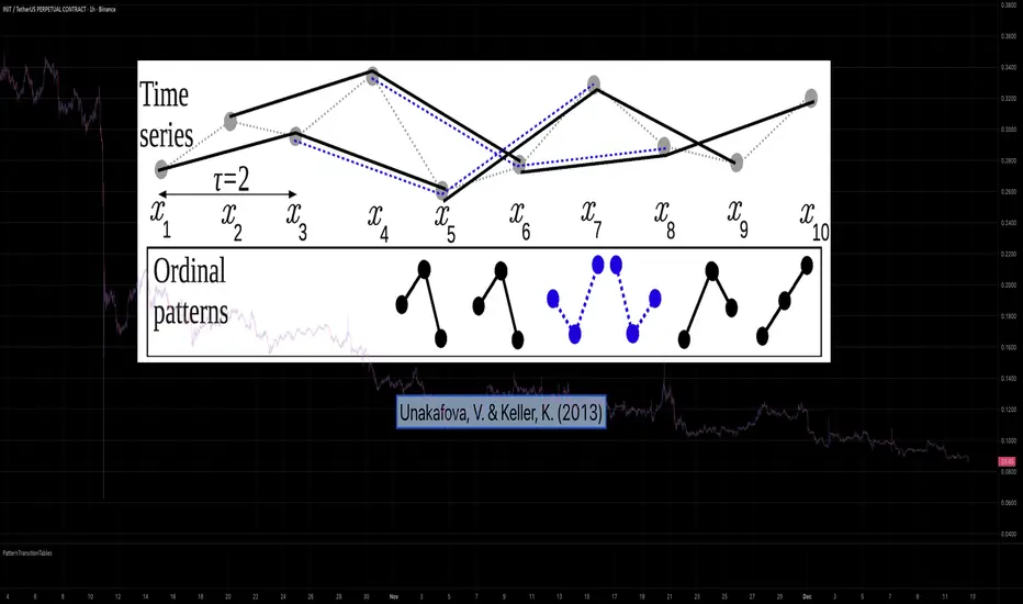
This library provides precomputed state transition tables to enable ultra-efficient, O(1) computation of Ordinal Patterns. It is designed specifically to support high-performance indicators calculating Permutation Entropy and related complexity measures.
💮 The Problem & Solution
Calculating Permutation Entropy, as introduced by Bandt and Pompe (2002), typically requires computing ordinal patterns within a sliding window at every time step. The standard successive-pattern method (Equations 2+3 in the paper) requires ≤ 4d-1 operations per update.
Unakafova and Keller (2013) demonstrated that successive ordinal patterns "overlap" significantly. By knowing the current pattern index and the relative rank (position l) of just the single new data point, the next pattern index can be determined via a precomputed look-up table. Computing l still requires d comparisons, but the table lookup itself is O(1), eliminating the need for d multiplications and d additions. This reduces total operations from ≤ 4d-1 to ≤ 2d per update (Table 4). This library contains these precomputed tables for orders d = 2 through d = 5.
🌸 --------- 2. THEORETICAL BACKGROUND --------- 🌸
💮 Permutation Entropy
Bandt, C., & Pompe, B. (2002). Permutation entropy: A natural complexity measure for time series.
doi.org
This concept quantifies the complexity of a system by comparing the order of neighbouring values rather than their magnitudes. It is robust against noise and non-linear distortions, making it ideal for financial time series analysis.
💮 Efficient Computation
Unakafova, V. A., & Keller, K. (2013). Efficiently Measuring Complexity on the Basis of Real-World Data.
doi.org
This library implements the transition function φ_d(n, l) described in Equation 5 of the paper. It maps a current pattern index (n) and the position of the new value (l) to the successor pattern, reducing the complexity of updates to constant time O(1).
🌸 --------- 3. LIBRARY FUNCTIONALITY --------- 🌸
💮 Data Structure
The library stores transition matrices as flattened 1D integer arrays. These tables are mathematically rigorous representations of the factorial number system used to enumerate permutations.
💮 Core Function: get_successor()
This is the primary interface for the library for direct pattern updates.
• Input: The current pattern index and the rank position of the incoming price data.
• Process: Routes the request to the specific transition table for the chosen order (d=2 to d=5).
• Output: The integer index of the next ordinal pattern.
💮 Table Access: get_table()
This function returns the entire flattened transition table for a specified dimension. This enables local caching of the table (e.g. in an indicator's init() method), avoiding the overhead of repeated library calls during the calculation loop.
💮 Supported Orders & Terminology
The parameter d is the order of ordinal patterns (following Bandt & Pompe 2002). Each pattern of order d contains (d+1) data points, yielding (d+1)! unique patterns:
• d=2: 3 points → 6 unique patterns, 3 successor positions
• d=3: 4 points → 24 unique patterns, 4 successor positions
• d=4: 5 points → 120 unique patterns, 5 successor positions
• d=5: 6 points → 720 unique patterns, 6 successor positions
Note: d=6 is not implemented. The resulting code size (approx. 191k tokens) exceeds the Pine Script limit of 100k tokens (as of 2025-12).
[GYTS-CE] Market Regime Detector🧊 Market Regime Detector (Community Edition)
🌸 Part of GoemonYae Trading System (GYTS) 🌸
🌸 --------- INTRODUCTION --------- 🌸
💮 What is the Market Regime Detector?
The Market Regime Detector is an advanced, consensus-based indicator that identifies the current market state to increase the probability of profitable trades. By distinguishing between trending (bullish or bearish) and cyclic (range-bound) market conditions, this detector helps you select appropriate tactics for different environments. Instead of forcing a single strategy across all market conditions, our detector allows you to adapt your approach based on real-time market behaviour.
💮 The Importance of Market Regimes
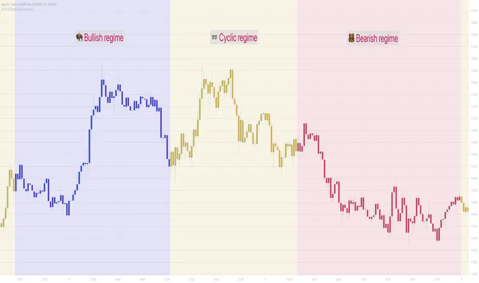
Markets constantly shift between different behavioural states or "regimes":
• Bullish trending markets - characterised by sustained upward price movement
• Bearish trending markets - characterised by sustained downward price movement
• Cyclic markets - characterised by range-bound, oscillating behaviour
Each regime requires fundamentally different trading approaches. Trend-following strategies excel in trending markets but fail in cyclic ones, while mean-reversion strategies shine in cyclic markets but underperform in trending conditions. Detecting these regimes is essential for successful trading, which is why we've developed the Market Regime Detector to accurately identify market states using complementary detection methods.
🌸 --------- KEY FEATURES --------- 🌸
💮 Consensus-Based Detection
Rather than relying on a single method, our detector employs two complementary detection methodologies that analyse different aspects of market behaviour:
• Dominant Cycle Average (DCA) - analyzes price movement relative to its lookback period, a proxy for the dominant cycle
• Volatility Channel - examines price behaviour within adaptive volatility bands
These diverse perspectives are synthesised into a robust consensus that minimises false signals while maintaining responsiveness to genuine regime changes.
💮 Dominant Cycle Framework
The Market Regime Detector uses the concept of dominant cycles to establish a reference framework. You can input the dominant cycle period that best represents the natural rhythm of your market, providing a stable foundation for regime detection across different timeframes.
💮 Intuitive Parameter System
We've distilled complex technical parameters into intuitive controls that traders can easily understand:
• Adaptability - how quickly the detector responds to changing market conditions
• Sensitivity - how readily the detector identifies transitions between regimes
• Consensus requirement - how much agreement is needed among detection methods
This approach makes the detector accessible to traders of all experience levels while preserving the power of the underlying algorithms.
💮 Visual Market Feedback
The detector provides clear visual feedback about the current market regime through:
• Colour-coded chart backgrounds (purple shades for bullish, pink for bearish, yellow for cyclic)
• Colour-coded price bars
• Strength indicators showing the degree of consensus
• Customizable colour schemes to match your preferences or trading system
💮 Integration in the GYTS suite
The Market Regime Detector is compatible with the GYTS Suite , i.e. it passes the regime into the 🎼 Order Orchestrator where you can set how to trade the trending and cyclic regime.
🌸 --------- CONFIGURATION SETTINGS --------- 🌸
💮 Adaptability
Controls how quickly the Market Regime detector adapts to changing market conditions. You can see it as a low-frequency, long-term change parameter:
Very Low: Very slow adaptation, most stable but may miss regime changes
Low: Slower adaptation, more stability but less responsiveness
Normal: Balanced between stability and responsiveness
High: Faster adaptation, more responsive but less stable
Very High: Very fast adaptation, highly responsive but may generate false signals
This setting affects lookback periods and filter parameters across all detection methods.
💮 Sensitivity
Controls how sensitive the detector is to market regime transitions. This acts as a high-frequency, short-term change parameter:
Very Low: Requires substantial evidence to identify a regime change
Low: Less sensitive, reduces false signals but may miss some transitions
Normal: Balanced sensitivity suitable for most markets
High: More sensitive, detects subtle regime changes but may have more noise
Very High: Very sensitive, detects minor fluctuations but may produce frequent changes
This setting affects thresholds for regime detection across all methods.
💮 Dominant Cycle Period
This parameter allows you to specify the market's natural rhythm in bars. This represents a complete market cycle (up and down movement). Finding the right value for your specific market and timeframe might require some experimentation, but it's a crucial parameter that helps the detector accurately identify regime changes. Most of the times the cycle is between 20 and 40 bars.
💮 Consensus Mode
Determines how the signals from both detection methods are combined to produce the final market regime:
• Any Method (OR) : Signals bullish/bearish if either method detects that regime. If methods conflict (one bullish, one bearish), the stronger signal wins. More sensitive, catches more regime changes but may produce more false signals.
• All Methods (AND) : Signals only when both methods agree on the regime. More conservative, reduces false signals but might miss some legitimate regime changes.
• Weighted Decision : Balances both methods with equal weighting. Provides a middle ground between sensitivity and stability.
Each mode also calculates a continuous regime strength value that's used for colour intensity in the 'unconstrained' display mode.
💮 Display Mode
Choose how to display the market regime colours:
• Unconstrained regime: Shows the regime strength as a continuous gradient. This provides more nuanced visualisation where the intensity of the colour indicates the strength of the trend.
• Consensus only: Shows only the final consensus regime with fixed colours based on the detected regime type.
The background and bar colours will change to indicate the current market regime:
• Purple shades: Bullish trending market (darker purple indicates stronger bullish trend)
• Pink shades: Bearish trending market (darker pink indicates stronger bearish trend)
• Yellow: Cyclic (range-bound) market
💮 Custom Colour Options
The Market Regime Detector allows you to customize the colour scheme to match your personal preferences or to coordinate with other indicators:
• Use custom colours: Toggle to enable your own colour choices instead of the default scheme
• Transparency: Adjust the transparency level of all regime colours
• Bullish colours: Define custom colours for strong, medium, weak, and very weak bullish trends
• Bearish colours: Define custom colours for strong, medium, weak, and very weak bearish trends
• Cyclic colour: Define a custom colour for cyclic (range-bound) market conditions
🌸 --------- DETECTION METHODS --------- 🌸
💮 Dominant Cycle Average (DCA)
The Dominant Cycle Average method forms a key part of our detection system:
1. Theoretical Foundation :
The DCA method builds on cycle analysis and the observation that in trending markets, price consistently remains on one side of a moving average calculated using the dominant cycle period. In contrast, during cyclic markets, price oscillates around this average.
2. Calculation Process :
• We calculate a Simple Moving Average (SMA) using the specified lookback period - a proxy for the dominant cycle period
• We then analyse the proportion of time that price spends above or below this SMA over a lookback window. The theory is that the price should cross the SMA each half cycle, assuming that the dominant cycle period is correct and price follows a sinusoid.
• This lookback window is adaptive, scaling with the dominant cycle period (controlled by the Adaptability setting)
• The different values are standardised and normalised to possess more resolving power and to be more robust to noise.
3. Regime Classification :
• When the normalised proportion exceeds a positive threshold (determined by Sensitivity setting), the market is classified as bullish trending
• When it falls below a negative threshold, the market is classified as bearish trending
• When the proportion remains between these thresholds, the market is classified as cyclic
💮 Volatility Channel
The Volatility Channel method complements the DCA method by focusing on price movement relative to adaptive volatility bands:
1. Theoretical Foundation :
This method is based on the observation that trending markets tend to sustain movement outside of normal volatility ranges, while cyclic markets tend to remain contained within these ranges. By creating adaptive bands that adjust to current market volatility, we can detect when price behaviour indicates a trending or cyclic regime.
2. Calculation Process :
• We first calculate a smooth base channel center using a low pass filter, creating a noise-reduced centreline for price
• True Range (TR) is used to measure market volatility, which is then smoothed and scaled by the deviation factor (controlled by Sensitivity)
• Upper and lower bands are created by adding and subtracting this scaled volatility from the centreline
• Price is smoothed using an adaptive A2RMA filter, which has a very flat and stable behaviour, to reduce noise while preserving trend characteristics
• The position of this smoothed price relative to the bands is continuously monitored
3. Regime Classification :
• When smoothed price moves above the upper band, the market is classified as bullish trending
• When smoothed price moves below the lower band, the market is classified as bearish trending
• When price remains between the bands, the market is classified as cyclic
• The magnitude of price's excursion beyond the bands is used to determine trend strength
4. Adaptive Behaviour :
• The smoothing periods and deviation calculations automatically adjust based on the Adaptability setting
• The measured volatility is calculated over a period proportional to the dominant cycle, ensuring the detector works across different timeframes
• Both the center line and the bands adapt dynamically to changing market conditions, making the detector responsive yet stable
This method provides a unique perspective that complements the DCA approach, with the consensus mechanism synthesising insights from both methods.
🌸 --------- USAGE GUIDE --------- 🌸
💮 Starting with Default Settings
The default settings (Normal for Adaptability and Sensitivity, Weighted Decision for Consensus Mode) provide a balanced starting point suitable for most markets and timeframes. Begin by observing how these settings identify regimes in your preferred instruments.
💮 Finding the Optimal Dominant Cycle
The dominant cycle period is a critical parameter. Here are some approaches to finding an appropriate value:
• Start with typical values, usually something around 25 works well
• Visually identify the average distance between significant peaks and troughs
• Experiment with different values and observe which provides the most stable regime identification
• Consider using cycle-finding indicators to help identify the natural rhythm of your market
💮 Adjusting Parameters
• If you notice too many regime changes → Decrease Sensitivity or increase Consensus requirement
• If regime changes seem delayed → Increase Adaptability
• If a trending regime is not detected, the market is automatically assigned to be in a cyclic state
• If you want to see more nuanced regime transitions → Try the "unconstrained" display mode (note that this will not affect the output to other indicators)
💮 Trading Applications
Regime-Specific Strategies:
• Bullish Trending Regime - Use trend-following strategies, trail stops wider, focus on breakouts, consider holding positions longer, and emphasize buying dips
• Bearish Trending Regime - Consider shorts, tighter stops, focus on breakdown points, sell rallies, implement downside protection, and reduce position sizes
• Cyclic Regime - Apply mean-reversion strategies, trade range boundaries, apply oscillators, target definable support/resistance levels, and use profit-taking at extremes
Strategy Switching:
Create a set of rules for each market regime and switch between them based on the detector's signal. This approach can significantly improve performance compared to applying a single strategy across all market conditions.
GYTS Suite Integration:
• In the GYTS 🎼 Order Orchestrator, select the '🔗 STREAM-int 🧊 Market Regime' as the market regime source
• Note that the consensus output (i.e. not the "unconstrained" display) will be used in this stream
• Create different strategies for trending (bullish/bearish) and cyclic regimes. The GYTS 🎼 Order Orchestrator is specifically made for this.
• The output stream is actually very simple, and can possibly be used in indicators and strategies as well. It outputs 1 for bullish, -1 for bearish and 0 for cyclic regime.
🌸 --------- FINAL NOTES --------- 🌸
💮 Development Philosophy
The Market Regime Detector has been developed with several key principles in mind:
1. Robustness - The detection methods have been rigorously tested across diverse markets and timeframes to ensure reliable performance.
2. Adaptability - The detector automatically adjusts to changing market conditions, requiring minimal manual intervention.
3. Complementarity - Each detection method provides a unique perspective, with the collective consensus being more reliable than any individual method.
4. Intuitiveness - Complex technical parameters have been abstracted into easily understood controls.
💮 Ongoing Refinement
The Market Regime Detector is under continuous development. We regularly:
• Fine-tune parameters based on expanded market data
• Research and integrate new detection methodologies
• Optimise computational efficiency for real-time analysis
Your feedback and suggestions are very important in this ongoing refinement process!
[GYTS] Filters ToolkitFilters Toolkit indicator
🌸 Part of GoemonYae Trading System (GYTS) 🌸
🌸 --------- 1. INTRODUCTION --------- 🌸
💮 Overview
The GYTS Filters Toolkit indicator is an advanced, interactive interface built atop the high‐performance, curated functions provided by the FiltersToolkit library . It allows traders to experiment with different combinations of filtering methods -— from smoothing low-pass filters to aggressive detrenders. With this toolkit, you can build custom indicators tailored to your specific trading strategy, whether you're looking for trend following, mean reversion, or cycle identification approaches.
🌸 --------- 2. FILTER METHODS AND TYPES --------- 🌸
💮 Filter categories
The available filters fall into four main categories, each marked with a distinct symbol:
🌗 Low Pass Filters (Smoothers)
These filters attenuate high-frequency components (noise) while allowing low-frequency components (trends) to pass through. Examples include:
Ultimate Smoother
Super Smoother (2-pole and 3-pole variants)
MESA Adaptive Moving Average (MAMA) and Following Adaptive Moving Average (FAMA)
BiQuad Low Pass Filter
ADXvma (Adaptive Directional Volatility Moving Average)
A2RMA (Adaptive Autonomous Recursive Moving Average)
Low pass filters are displayed on the price chart by default, as they follow the overall price movement. If they are combined with a high-pass or bandpass filter, they will be displayed in the subgraph.
🌓 High Pass Filters (Detrenders)
These filters do the opposite of low pass filters - they remove low-frequency components (trends) while allowing high-frequency components to pass through. Examples include:
Butterworth High Pass Filter
BiQuad High Pass Filter
High pass filters are displayed as oscillators in the subgraph below the price chart, as they fluctuate around a zero line.
🌑 Band Pass Filters (Cycle Isolators)
These filters combine aspects of both low and high pass filters, isolating specific frequency ranges while attenuating both higher and lower frequencies. Examples include:
Ehlers Bandpass Filter
Cyber Cycle
Relative Vigor Index (RVI)
BiQuad Bandpass Filter
Band pass filters are also displayed as oscillators in a separate panel.
🔮 Predictive Filter
Voss Predictive Filter: A special filter that attempts to predict future values of band-limited signals (only to be used as post-filter). Keep its prediction horizon short (1–3 bars) for reasonable accuracy.
Note that the the library contains elaborate documentation and source material of each filter.
🌸 --------- 3. INDICATOR FEATURES --------- 🌸
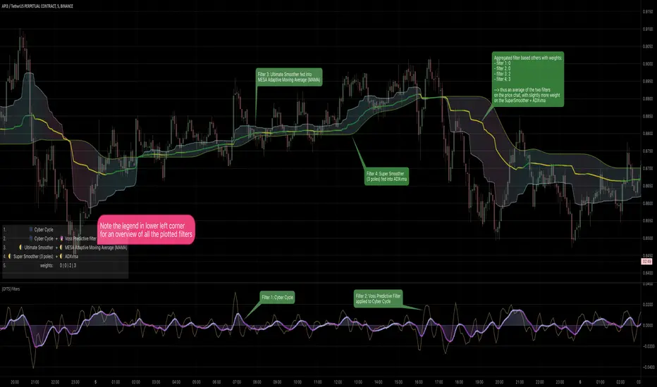
💮 Multi-filter configuration
One of the most powerful aspects of this indicator is the ability to configure multiple filters. compare them and observe their combined effects. There are four primary filters, each with its own parameter settings.
💮 Post-filtering
Process a filter’s output through an additional filter by enabling the post-filter option. This creates a filter chain where the output of one filter becomes the input to another. Some powerful combinations include:
Ultimate Smoother → MAMA: Creates an adaptive smoothing effect that responds well to market changes, good for trend-following strategies
Butterworth → Super Smoother → Butterworth: Produces a well-behaved oscillator with minimal phase distortion, John Ehlers also calls a "roofing filter". Great for identifying overbought/oversold conditions with minimal lag.
A bandpass filter → Voss Prediction filter: Attempts to predict future movements of cyclical components, handy to find peaks and troughs of the market cycle.
💮 Aggregate filters
Arguably the coolest feature: aggregating filters allow you to combine multiple filters with different weights. Important notes about aggregation:
You can only aggregate filters that appear on the same chart (price chart or oscillator panel).
The weights are automatically normalised, so only their relative values matter
Setting a weight to 0 (zero) excludes that filter from the aggregation
Filters don't need to be visibly displayed to be included in aggregation
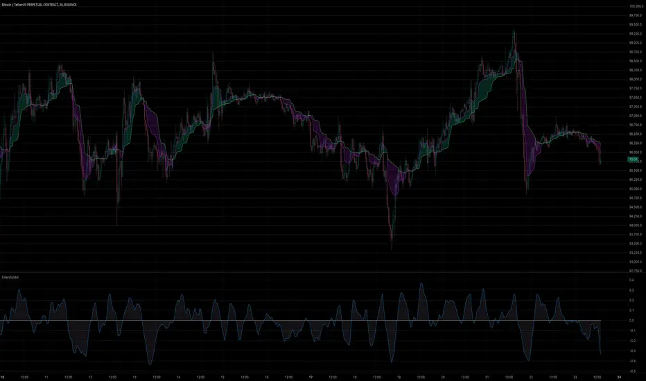
💮 Rich visualisation & alerts
The indicator intelligently determines whether a filter is displayed on the price chart or in the subgraph (as an oscillator) based on its characteristics.
Dynamic colour palettes, adjustable line widths, transparency, and custom fill between any of enabled filters or between oscillators and the zero-line.
A clear legend showing which filters are active and how they're configured
Alerts for direction changes and crossovers of all filters
🌸 --------- 4. ACKNOWLEDGEMENTS --------- 🌸
This toolkit builds on the work of numerous pioneers in technical analysis and digital signal processing:
John Ehlers, whose groundbreaking research forms the foundation of many filters.
Robert Bristow-Johnson for the BiQuad filter formulations.
The TradingView community, especially @The_Peaceful_Lizard, @alexgrover, and others mentioned in the code of the library.
Everyone who has provided feedback, testing and support!
[GYTS] FiltersToolkit LibraryFiltersToolkit Library
🌸 Part of GoemonYae Trading System (GYTS) 🌸
🌸 --------- 1. INTRODUCTION --------- 🌸
💮 What Does This Library Contain?
This library is a curated collection of high-performance digital signal processing (DSP) filters and auxiliary functions designed specifically for financial time series analysis. It includes a shortlist of our favourite and best performing filters — each rigorously tested and selected for their responsiveness, minimal lag and robustness in diverse market conditions. These tools form an integral part of the GoemonYae Trading System (GYTS), chosen for their unique characteristics in handling market data.
The library contains two main categories:
1. Smoothing filters (low-pass filters and moving averages) for e.g. denoising, trend following
2. Detrending tools (high-pass and band-pass filters, known as "oscillators") for e.g. mean reversion
This collection is finely tuned for practical trading applications and is therefore not meant to be exhaustive. However, will continue to expand as we discover and validate new filtering techniques. I welcome collaboration and suggestions for novel approaches.
🌸 ——— 2. ADDED VALUE ——— 🌸
💮 Unified syntax and comprehensive documentation
The FiltersToolkit Library brings together a wide array of valuable filters under a unified, intuitive syntax. Each function is thoroughly documented, with clear explanations and academic sources that underline the mathematical rigour behind the methods. This level of documentation not only facilitates integration into trading strategies but also helps underlying the underlying concepts and rationale.
💮 Optimised performance and readability
The code prioritizes computational efficiency while maintaining readability. Key optimizations include:
- Minimizing redundant calculations in recursive filters
- Smart coefficient caching
- Efficient state management
- Vectorized operations where applicable
💮 Enhanced functionality and flexibility
Some filters in this library introduce extended functionality beyond the original publications. For instance, the MESA Adaptive Moving Average (MAMA) and Ehlers’ Combined Bandpass Filter incorporate multiple variations found in the literature, thereby providing traders with flexible tools that can be fine-tuned to different market conditions.
🌸 ——— 3. THE FILTERS ——— 🌸
💮 Hilbert Transform Function
This function implements the Hilbert Transform as utilised by John Ehlers. It converts a real-valued time series into its analytic signal, enabling the extraction of instantaneous phase and frequency information—an essential step in adaptive filtering.
Source: John Ehlers - "Rocket Science for Traders" (2001), "TASC 2001 V. 19:9", "Cybernetic Analysis for Stocks and Futures" (2004)
💮 Homodyne Discriminator
By leveraging the Hilbert Transform, this function computes the dominant cycle period through a Homodyne Discriminator. It extracts the in-phase and quadrature components of the signal, facilitating a robust estimation of the underlying cycle characteristics.
Source: John Ehlers - "Rocket Science for Traders" (2001), "TASC 2001 V. 19:9", "Cybernetic Analysis for Stocks and Futures" (2004)
💮 MESA Adaptive Moving Average (MAMA)
An advanced dual-stage adaptive moving average, this function outputs both the MAMA and its companion FAMA. It combines adaptive alpha computation with elements from Kaufman’s Adaptive Moving Average (KAMA) to provide a responsive and reliable trend indicator.
Source: John Ehlers - "Rocket Science for Traders" (2001), "TASC 2001 V. 19:9", "Cybernetic Analysis for Stocks and Futures" (2004)
💮 BiQuad Filters
A family of second-order recursive filters offering exceptional control over frequency response:
- High-pass filter for detrending
- Low-pass filter for smooth trend following
- Band-pass filter for cycle isolation
The quality factor (Q) parameter allows fine-tuning of the resonance characteristics, making these filters highly adaptable to different market conditions.
Source: Robert Bristow-Johnson's Audio EQ Cookbook, implemented by @The_Peaceful_Lizard
💮 Relative Vigor Index (RVI)
This filter evaluates the strength of a trend by comparing the closing price to the trading range. Operating similarly to a band-pass filter, the RVI provides insights into market momentum and potential reversals.
Source: John Ehlers – “Cybernetic Analysis for Stocks and Futures” (2004)
💮 Cyber Cycle
The Cyber Cycle filter emphasises market cycles by smoothing out noise and highlighting the dominant cyclical behaviour. It is particularly useful for detecting trend reversals and cyclical patterns in the price data.
Source: John Ehlers – “Cybernetic Analysis for Stocks and Futures” (2004)
💮 Butterworth High Pass Filter
Inspired by the classical Butterworth design, this filter achieves a maximally flat magnitude response in the passband while effectively removing low-frequency trends. Its design minimises phase distortion, which is vital for accurate signal interpretation.
Source: John Ehlers – “Cybernetic Analysis for Stocks and Futures” (2004)
💮 2-Pole SuperSmoother
Employing a two-pole design, the SuperSmoother filter reduces high-frequency noise with minimal lag. It is engineered to preserve trend integrity while offering a smooth output even in noisy market conditions.
Source: John Ehlers – “Cybernetic Analysis for Stocks and Futures” (2004)
💮 3-Pole SuperSmoother
An extension of the 2-pole design, the 3-pole SuperSmoother further attenuates high-frequency noise. Its additional pole delivers enhanced smoothing at the cost of slightly increased lag.
Source: John Ehlers – “Cybernetic Analysis for Stocks and Futures” (2004)
💮 Adaptive Directional Volatility Moving Average (ADXVma)
This adaptive moving average adjusts its smoothing factor based on directional volatility. By combining true range and directional movement measurements, it remains exceptionally flat during ranging markets and responsive during directional moves.
Source: Various implementations across platforms, unified and optimized
💮 Ehlers Combined Bandpass Filter with Automated Gain Control (AGC)
This sophisticated filter merges a highpass pre-processing stage with a bandpass filter. An integrated Automated Gain Control normalises the output to a consistent range, while offering both regular and truncated recursive formulations to manage lag.
Source: John F. Ehlers – “Truncated Indicators” (2020), “Cycle Analytics for Traders” (2013)
💮 Voss Predictive Filter
A forward-looking filter that predicts future values of a band-limited signal in real time. By utilising multiple time-delayed feedback terms, it provides anticipatory coupling and delivers a short-term predictive signal.
Source: John Ehlers - "A Peek Into The Future" (TASC 2019-08)
💮 Adaptive Autonomous Recursive Moving Average (A2RMA)
This filter dynamically adjusts its smoothing through an adaptive mechanism based on an efficiency ratio and a dynamic threshold. A double application of an adaptive moving average ensures both responsiveness and stability in volatile and ranging markets alike. Very flat response when properly tuned.
Source: @alexgrover (2019)
💮 Ultimate Smoother (2-Pole)
The Ultimate Smoother filter is engineered to achieve near-zero lag in its passband by subtracting a high-pass response from an all-pass response. This creates a filter that maintains signal fidelity at low frequencies while effectively filtering higher frequencies at the expense of slight overshooting.
Source: John Ehlers - TASC 2024-04 "The Ultimate Smoother"
Note: This library is actively maintained and enhanced. Suggestions for additional filters or improvements are welcome through the usual channels. The source code contains a list of tested filters that did not make it into the curated collection.
ColourUtilitiesLibrary "ColourUtilities"
Utility functions for colour manipulation
adjust_colour(rgb, desaturation_amount, transparency_amount)
to reduce saturation or increase transparency of an RGB colour
Parameters:
rgb (color)
desaturation_amount (float) : 0 means no desaturation (colours remains as-is), and 1 means full desaturation (colour turns grey). Can also be used inversely with negative numbers
transparency_amount (float) : How much more transparent the default transparency should become. E.g. with a value of 0.5, a transparency of 0 becomes 50 and 40 becomes 70. A value of 1 makes it fully transparent, en -1 fully opaque.
Returns: color with adjusted saturation and transparency
method apply_default_palette(self, palette_name)
Some nice looking colour palettes, consisting of 6 gradient colours, are already defined here and can be quickly applied to the Palette class
Namespace types: Palette
Parameters:
self (Palette)
palette_name (string) : Currently there are 4 6-coloured palettes available: "GYTS flux signal", "GYTS purple", "GYTS flux filter" and "GYTS maroon"
Returns: None, as it populates the Palette class with pre-defined colours
method get_colour(self, colour_no, transparency)
Retrieves colour from the palette and possibly changes transparency if set
Namespace types: Palette
Parameters:
self (Palette)
colour_no (int) : from the palette
transparency (int) : to possibly change the default transparency of the palette
Returns: colour
method get_dynamic_colour(self, x, mid_point, colour_lb, colour_ub, trend_lookback, use_rate)
Retrieves a colour based on strength and direction of the passed series
Namespace types: Palette
Parameters:
self (Palette)
x (float) : the input data series
mid_point (float) : value as a cutoff point where the bullish/bearish colour scenario
colour_lb (float) : value (lower bound) where to apply the bearish colour at full strength
colour_ub (float) : value (upper bound) where to apply the bullish colour at full strength
trend_lookback (int) : how much bars back to check if there was a consistent move into a certain direction, otherwise a the neutral colour from the centre of the palette will be used.
use_rate (bool) : whether to use the rate (proportional difference with previous `x` value) or the input series `x` directly
Returns: colour
Palette
Fields:
transparency (series__integer)
palette (array__color)
