PnL Bubble [%] | Fractalyst1. What's the indicator purpose?
The PnL Bubble indicator transforms your strategy's trade PnL percentages into an interactive bubble chart with professional-grade statistics and performance analytics. It helps traders quickly assess system profitability, understand win/loss distribution patterns, identify outliers, and make data-driven strategy improvements.
How does it work?
Think of this indicator as a visual report card for your trading performance. Here's what it does:
What You See
Colorful Bubbles: Each bubble represents one of your trades
Blue/Cyan bubbles = Winning trades (you made money)
Red bubbles = Losing trades (you lost money)
Bigger bubbles = Bigger wins or losses
Smaller bubbles = Smaller wins or losses
How It Organizes Your Trades:
Like a Photo Album: Instead of showing all your trades at once (which would be messy), it shows them in "pages" of 500 trades each:
Page 1: Your first 500 trades
Page 2: Trades 501-1000
Page 3: Trades 1001-1500, etc.
What the Numbers Tell You:
Average Win: How much money you typically make on winning trades
Average Loss: How much money you typically lose on losing trades
Expected Value (EV): Whether your trading system makes money over time
Positive EV = Your system is profitable long-term
Negative EV = Your system loses money long-term
Payoff Ratio (R): How your average win compares to your average loss
R > 1 = Your wins are bigger than your losses
R < 1 = Your losses are bigger than your wins
Why This Matters:
At a Glance: You can instantly see if you're a profitable trader or not
Pattern Recognition: Spot if you have more big wins than big losses
Performance Tracking: Watch how your trading improves over time
Realistic Expectations: Understand what "average" performance looks like for your system
The Cool Visual Effects:
Animation: The bubbles glow and shimmer to make the chart more engaging
Highlighting: Your biggest wins and losses get extra attention with special effects
Tooltips: hover any bubble to see details about that specific trade.
What are the underlying calculations?
The indicator processes trade PnL data using a dual-matrix architecture for optimal performance:
Dual-Matrix System:
• Display Matrix (display_matrix): Bounded to 500 trades for rendering performance
• Statistics Matrix (stats_matrix): Unbounded storage for complete statistical accuracy
Trade Classification & Aggregation:
// Separate wins, losses, and break-even trades
if val > 0.0
pos_sum += val // Sum winning trades
pos_count += 1 // Count winning trades
else if val < 0.0
neg_sum += val // Sum losing trades
neg_count += 1 // Count losing trades
else
zero_count += 1 // Count break-even trades
Statistical Averages:
avg_win = pos_count > 0 ? pos_sum / pos_count : na
avg_loss = neg_count > 0 ? math.abs(neg_sum) / neg_count : na
Win/Loss Rates:
total_obs = pos_count + neg_count + zero_count
win_rate = pos_count / total_obs
loss_rate = neg_count / total_obs
Expected Value (EV):
ev_value = (avg_win × win_rate) - (avg_loss × loss_rate)
Payoff Ratio (R):
R = avg_win ÷ |avg_loss|
Contribution Analysis:
ev_pos_contrib = avg_win × win_rate // Positive EV contribution
ev_neg_contrib = avg_loss × loss_rate // Negative EV contribution
How to integrate with any trading strategy?
Equity Change Tracking Method:
//@version=6
strategy("Your Strategy with Equity Change Export", overlay=true)
float prev_trade_equity = na
float equity_change_pct = na
if barstate.isconfirmed and na(prev_trade_equity)
prev_trade_equity := strategy.equity
trade_just_closed = strategy.closedtrades != strategy.closedtrades
if trade_just_closed and not na(prev_trade_equity)
current_equity = strategy.equity
equity_change_pct := ((current_equity - prev_trade_equity) / prev_trade_equity) * 100
prev_trade_equity := current_equity
else
equity_change_pct := na
plot(equity_change_pct, "Equity Change %", display=display.data_window)
Integration Steps:
1. Add equity tracking code to your strategy
2. Load both strategy and PnL Bubble indicator on the same chart
3. In bubble indicator settings, select your strategy's equity tracking output as data source
4. Configure visualization preferences (colors, effects, page navigation)
How does the pagination system work?
The indicator uses an intelligent pagination system to handle large trade datasets efficiently:
Page Organization:
• Page 1: Trades 1-500 (most recent)
• Page 2: Trades 501-1000
• Page 3: Trades 1001-1500
• Page N: Trades to
Example: With 1,500 trades total (3 pages available):
• User selects Page 1: Shows trades 1-500
• User selects Page 4: Automatically falls back to Page 3 (trades 1001-1500)
5. Understanding the Visual Elements
Bubble Visualization:
• Color Coding: Cyan/blue gradients for wins, red gradients for losses
• Size Mapping: Bubble size proportional to trade magnitude (larger = bigger P&L)
• Priority Rendering: Largest trades displayed first to ensure visibility
• Gradient Effects: Color intensity increases with trade magnitude within each category
Interactive Tooltips:
Each bubble displays quantitative trade information:
tooltip_text = outcome + " | PnL: " + pnl_str +
" Date: " + date_str + " " + time_str +
" Trade #" + str.tostring(trade_number) + " (Page " + str.tostring(active_page) + ")" +
" Rank: " + str.tostring(rank) + " of " + str.tostring(n_display_rows) +
" Percentile: " + str.tostring(percentile, "#.#") + "%" +
" Magnitude: " + str.tostring(magnitude_pct, "#.#") + "%"
Example Tooltip:
Win | PnL: +2.45%
Date: 2024.03.15 14:30
Trade #1,247 (Page 3)
Rank: 5 of 347
Percentile: 98.6%
Magnitude: 85.2%
Reference Lines & Statistics:
• Average Win Line: Horizontal reference showing typical winning trade size
• Average Loss Line: Horizontal reference showing typical losing trade size
• Zero Line: Threshold separating wins from losses
• Statistical Labels: EV, R-Ratio, and contribution analysis displayed on chart
What do the statistical metrics mean?
Expected Value (EV):
Represents the mathematical expectation per trade in percentage terms
EV = (Average Win × Win Rate) - (Average Loss × Loss Rate)
Interpretation:
• EV > 0: Profitable system with positive mathematical expectation
• EV = 0: Break-even system, profitability depends on execution
• EV < 0: Unprofitable system with negative mathematical expectation
Example: EV = +0.34% means you expect +0.34% profit per trade on average
Payoff Ratio (R):
Quantifies the risk-reward relationship of your trading system
R = Average Win ÷ |Average Loss|
Interpretation:
• R > 1.0: Wins are larger than losses on average (favorable risk-reward)
• R = 1.0: Wins and losses are equal in magnitude
• R < 1.0: Losses are larger than wins on average (unfavorable risk-reward)
Example: R = 1.5 means your average win is 50% larger than your average loss
Contribution Analysis (Σ):
Breaks down the components of expected value
Positive Contribution (Σ+) = Average Win × Win Rate
Negative Contribution (Σ-) = Average Loss × Loss Rate
Purpose:
• Shows how much wins contribute to overall expectancy
• Shows how much losses detract from overall expectancy
• Net EV = Σ+ - Σ- (Expected Value per trade)
Example: Σ+: 1.23% means wins contribute +1.23% to expectancy
Example: Σ-: -0.89% means losses drag expectancy by -0.89%
Win/Loss Rates:
Win Rate = Count(Wins) ÷ Total Trades
Loss Rate = Count(Losses) ÷ Total Trades
Shows the probability of winning vs losing trades
Higher win rates don't guarantee profitability if average losses exceed average wins
7. Demo Mode & Synthetic Data Generation
When using built-in sources (close, open, etc.), the indicator generates realistic demo trades for testing:
if isBuiltInSource(source_data)
// Generate random trade outcomes with realistic distribution
u_sign = prand(float(time), float(bar_index))
if u_sign < 0.5
v_push := -1.0 // Loss trade
else
// Skewed distribution favoring smaller wins (realistic)
u_mag = prand(float(time) + 9876.543, float(bar_index) + 321.0)
k = 8.0 // Skewness factor
t = math.pow(u_mag, k)
v_push := 2.5 + t * 8.0 // Win trade
Demo Characteristics:
• Realistic win/loss distribution mimicking actual trading patterns
• Skewed distribution favoring smaller wins over large wins
• Deterministic randomness for consistent demo results
• Includes jitter effects to prevent visual overlap
8. Performance Limitations & Optimizations
Display Constraints:
points_count = 500 // Maximum 500 dots per page for optimal performance
Pine Script v6 Limits:
• Label Count: Maximum 500 labels per indicator
• Line Count: Maximum 100 lines per indicator
• Box Count: Maximum 50 boxes per indicator
• Matrix Size: Efficient memory management with dual-matrix system
Optimization Strategies:
• Pagination System: Handle unlimited trades through 500-trade pages
• Priority Rendering: Largest trades displayed first for maximum visibility
• Dual-Matrix Architecture: Separate display (bounded) from statistics (unbounded)
• Smart Fallback: Automatic page clamping prevents empty displays
Impact & Workarounds:
• Visual Limitation: Only 500 trades visible per page
• Statistical Accuracy: Complete dataset used for all calculations
• Navigation: Use page input to browse through entire trade history
• Performance: Smooth operation even with thousands of trades
9. Statistical Accuracy Guarantees
Data Integrity:
• Complete Dataset: Statistics matrix stores ALL trades without limit
• Proper Aggregation: Separate tracking of wins, losses, and break-even trades
• Mathematical Precision: Pine Script v6's enhanced floating-point calculations
• Dual-Matrix System: Display limitations don't affect statistical accuracy
Calculation Validation:
// Verified formulas match standard trading mathematics
avg_win = pos_sum / pos_count // Standard average calculation
win_rate = pos_count / total_obs // Standard probability calculation
ev_value = (avg_win * win_rate) - (avg_loss * loss_rate) // Standard EV formula
Accuracy Features:
• Mathematical Correctness: Formulas follow established trading statistics
• Data Preservation: Complete dataset maintained for all calculations
• Precision Handling: Proper rounding and boundary condition management
• Real-Time Updates: Statistics recalculated on every new trade
10. Advanced Technical Features
Real-Time Animation Engine:
// Shimmer effects with sine wave modulation
offset = math.sin(shimmer_t + phase) * amp
// Dynamic transparency with organic flicker
new_transp = math.min(flicker_limit, math.max(-flicker_limit, cur_transp + dir * flicker_step))
• Sine Wave Shimmer: Dynamic glowing effects on bubbles
• Organic Flicker: Random transparency variations for natural feel
• Extreme Value Highlighting: Special visual treatment for outliers
• Smooth Animations: Tick-based updates for fluid motion
Magnitude-Based Priority Rendering:
// Sort trades by magnitude for optimal visual hierarchy
sort_indices_by_magnitude(values_mat)
• Largest First: Most important trades always visible
• Intelligent Sorting: Custom bubble sort algorithm for trade prioritization
• Performance Optimized: Efficient sorting for real-time updates
• Visual Hierarchy: Ensures critical trades never get hidden
Professional Tooltip System:
• Quantitative Data: Pure numerical information without interpretative language
• Contextual Ranking: Shows trade position within page dataset
• Percentile Analysis: Performance ranking as percentage
• Magnitude Scaling: Relative size compared to page maximum
• Professional Format: Clean, data-focused presentation
11. Quick Start Guide
Step 1: Add Indicator
• Search for "PnL Bubble | Fractalyst" in TradingView indicators
• Add to your chart (works on any timeframe)
Step 2: Configure Data Source
• Demo Mode: Leave source as "close" to see synthetic trading data
• Strategy Mode: Select your strategy's PnL% output as data source
Step 3: Customize Visualization
• Colors: Set positive (cyan), negative (red), and neutral colors
• Page Navigation: Use "Trade Page" input to browse trade history
• Visual Effects: Built-in shimmer and animation effects are enabled by default
Step 4: Analyze Performance
• Study bubble patterns for win/loss distribution
• Review statistical metrics: EV, R-Ratio, Win Rate
• Use tooltips for detailed trade analysis
• Navigate pages to explore full trade history
Step 5: Optimize Strategy
• Identify outlier trades (largest bubbles)
• Analyze risk-reward profile through R-Ratio
• Monitor Expected Value for system profitability
• Use contribution analysis to understand win/loss impact
12. Why Choose PnL Bubble Indicator?
Unique Advantages:
• Advanced Pagination: Handle unlimited trades with smart fallback system
• Dual-Matrix Architecture: Perfect balance of performance and accuracy
• Professional Statistics: Institution-grade metrics with complete data integrity
• Real-Time Animation: Dynamic visual effects for engaging analysis
• Quantitative Tooltips: Pure numerical data without subjective interpretations
• Priority Rendering: Intelligent magnitude-based display ensures critical trades are always visible
Technical Excellence:
• Built with Pine Script v6 for maximum performance and modern features
• Optimized algorithms for smooth operation with large datasets
• Complete statistical accuracy despite display optimizations
• Professional-grade calculations matching institutional trading analytics
Practical Benefits:
• Instantly identify system profitability through visual patterns
• Spot outlier trades and risk management issues
• Understand true risk-reward profile of your strategies
• Make data-driven decisions for strategy optimization
• Professional presentation suitable for performance reporting
Disclaimer & Risk Considerations:
Important: Historical performance metrics, including positive Expected Value (EV), do not guarantee future trading success. Statistical measures are derived from finite sample data and subject to inherent limitations:
• Sample Bias: Historical data may not represent future market conditions or regime changes
• Ergodicity Assumption: Markets are non-stationary; past statistical relationships may break down
• Survivorship Bias: Strategies showing positive historical EV may fail during different market cycles
• Parameter Instability: Optimal parameters identified in backtesting often degrade in forward testing
• Transaction Cost Evolution: Slippage, spreads, and commission structures change over time
• Behavioral Factors: Live trading introduces psychological elements absent in backtesting
• Black Swan Events: Extreme market events can invalidate statistical assumptions instantaneously
Quanttrading

Markov Chain [3D] | FractalystWhat exactly is a Markov Chain?
This indicator uses a Markov Chain model to analyze, quantify, and visualize the transitions between market regimes (Bull, Bear, Neutral) on your chart. It dynamically detects these regimes in real-time, calculates transition probabilities, and displays them as animated 3D spheres and arrows, giving traders intuitive insight into current and future market conditions.
How does a Markov Chain work, and how should I read this spheres-and-arrows diagram?
Think of three weather modes: Sunny, Rainy, Cloudy.
Each sphere is one mode. The loop on a sphere means “stay the same next step” (e.g., Sunny again tomorrow).
The arrows leaving a sphere show where things usually go next if they change (e.g., Sunny moving to Cloudy).
Some paths matter more than others. A more prominent loop means the current mode tends to persist. A more prominent outgoing arrow means a change to that destination is the usual next step.
Direction isn’t symmetric: moving Sunny→Cloudy can behave differently than Cloudy→Sunny.
Now relabel the spheres to markets: Bull, Bear, Neutral.
Spheres: market regimes (uptrend, downtrend, range).
Self‑loop: tendency for the current regime to continue on the next bar.
Arrows: the most common next regime if a switch happens.
How to read: Start at the sphere that matches current bar state. If the loop stands out, expect continuation. If one outgoing path stands out, that switch is the typical next step. Opposite directions can differ (Bear→Neutral doesn’t have to match Neutral→Bear).
What states and transitions are shown?
The three market states visualized are:
Bullish (Bull): Upward or strong-market regime.
Bearish (Bear): Downward or weak-market regime.
Neutral: Sideways or range-bound regime.
Bidirectional animated arrows and probability labels show how likely the market is to move from one regime to another (e.g., Bull → Bear or Neutral → Bull).
How does the regime detection system work?
You can use either built-in price returns (based on adaptive Z-score normalization) or supply three custom indicators (such as volume, oscillators, etc.).
Values are statistically normalized (Z-scored) over a configurable lookback period.
The normalized outputs are classified into Bull, Bear, or Neutral zones.
If using three indicators, their regime signals are averaged and smoothed for robustness.
How are transition probabilities calculated?
On every confirmed bar, the algorithm tracks the sequence of detected market states, then builds a rolling window of transitions.
The code maintains a transition count matrix for all regime pairs (e.g., Bull → Bear).
Transition probabilities are extracted for each possible state change using Laplace smoothing for numerical stability, and frequently updated in real-time.
What is unique about the visualization?
3D animated spheres represent each regime and change visually when active.
Animated, bidirectional arrows reveal transition probabilities and allow you to see both dominant and less likely regime flows.
Particles (moving dots) animate along the arrows, enhancing the perception of regime flow direction and speed.
All elements dynamically update with each new price bar, providing a live market map in an intuitive, engaging format.
Can I use custom indicators for regime classification?
Yes! Enable the "Custom Indicators" switch and select any three chart series as inputs. These will be normalized and combined (each with equal weight), broadening the regime classification beyond just price-based movement.
What does the “Lookback Period” control?
Lookback Period (default: 100) sets how much historical data builds the probability matrix. Shorter periods adapt faster to regime changes but may be noisier. Longer periods are more stable but slower to adapt.
How is this different from a Hidden Markov Model (HMM)?
It sets the window for both regime detection and probability calculations. Lower values make the system more reactive, but potentially noisier. Higher values smooth estimates and make the system more robust.
How is this Markov Chain different from a Hidden Markov Model (HMM)?
Markov Chain (as here): All market regimes (Bull, Bear, Neutral) are directly observable on the chart. The transition matrix is built from actual detected regimes, keeping the model simple and interpretable.
Hidden Markov Model: The actual regimes are unobservable ("hidden") and must be inferred from market output or indicator "emissions" using statistical learning algorithms. HMMs are more complex, can capture more subtle structure, but are harder to visualize and require additional machine learning steps for training.
A standard Markov Chain models transitions between observable states using a simple transition matrix, while a Hidden Markov Model assumes the true states are hidden (latent) and must be inferred from observable “emissions” like price or volume data. In practical terms, a Markov Chain is transparent and easier to implement and interpret; an HMM is more expressive but requires statistical inference to estimate hidden states from data.
Markov Chain: states are observable; you directly count or estimate transition probabilities between visible states. This makes it simpler, faster, and easier to validate and tune.
HMM: states are hidden; you only observe emissions generated by those latent states. Learning involves machine learning/statistical algorithms (commonly Baum–Welch/EM for training and Viterbi for decoding) to infer both the transition dynamics and the most likely hidden state sequence from data.
How does the indicator avoid “repainting” or look-ahead bias?
All regime changes and matrix updates happen only on confirmed (closed) bars, so no future data is leaked, ensuring reliable real-time operation.
Are there practical tuning tips?
Tune the Lookback Period for your asset/timeframe: shorter for fast markets, longer for stability.
Use custom indicators if your asset has unique regime drivers.
Watch for rapid changes in transition probabilities as early warning of a possible regime shift.
Who is this indicator for?
Quants and quantitative researchers exploring probabilistic market modeling, especially those interested in regime-switching dynamics and Markov models.
Programmers and system developers who need a probabilistic regime filter for systematic and algorithmic backtesting:
The Markov Chain indicator is ideally suited for programmatic integration via its bias output (1 = Bull, 0 = Neutral, -1 = Bear).
Although the visualization is engaging, the core output is designed for automated, rules-based workflows—not for discretionary/manual trading decisions.
Developers can connect the indicator’s output directly to their Pine Script logic (using input.source()), allowing rapid and robust backtesting of regime-based strategies.
It acts as a plug-and-play regime filter: simply plug the bias output into your entry/exit logic, and you have a scientifically robust, probabilistically-derived signal for filtering, timing, position sizing, or risk regimes.
The MC's output is intentionally "trinary" (1/0/-1), focusing on clear regime states for unambiguous decision-making in code. If you require nuanced, multi-probability or soft-label state vectors, consider expanding the indicator or stacking it with a probability-weighted logic layer in your scripting.
Because it avoids subjectivity, this approach is optimal for systematic quants, algo developers building backtested, repeatable strategies based on probabilistic regime analysis.
What's the mathematical foundation behind this?
The mathematical foundation behind this Markov Chain indicator—and probabilistic regime detection in finance—draws from two principal models: the (standard) Markov Chain and the Hidden Markov Model (HMM).
How to use this indicator programmatically?
The Markov Chain indicator automatically exports a bias value (+1 for Bullish, -1 for Bearish, 0 for Neutral) as a plot visible in the Data Window. This allows you to integrate its regime signal into your own scripts and strategies for backtesting, automation, or live trading.
Step-by-Step Integration with Pine Script (input.source)
Add the Markov Chain indicator to your chart.
This must be done first, since your custom script will "pull" the bias signal from the indicator's plot.
In your strategy, create an input using input.source()
Example:
//@version=5
strategy("MC Bias Strategy Example")
mcBias = input.source(close, "MC Bias Source")
After saving, go to your script’s settings. For the “MC Bias Source” input, select the plot/output of the Markov Chain indicator (typically its bias plot).
Use the bias in your trading logic
Example (long only on Bull, flat otherwise):
if mcBias == 1
strategy.entry("Long", strategy.long)
else
strategy.close("Long")
For more advanced workflows, combine mcBias with additional filters or trailing stops.
How does this work behind-the-scenes?
TradingView’s input.source() lets you use any plot from another indicator as a real-time, “live” data feed in your own script (source).
The selected bias signal is available to your Pine code as a variable, enabling logical decisions based on regime (trend-following, mean-reversion, etc.).
This enables powerful strategy modularity : decouple regime detection from entry/exit logic, allowing fast experimentation without rewriting core signal code.
Integrating 45+ Indicators with Your Markov Chain — How & Why
The Enhanced Custom Indicators Export script exports a massive suite of over 45 technical indicators—ranging from classic momentum (RSI, MACD, Stochastic, etc.) to trend, volume, volatility, and oscillator tools—all pre-calculated, centered/scaled, and available as plots.
// Enhanced Custom Indicators Export - 45 Technical Indicators
// Comprehensive technical analysis suite for advanced market regime detection
//@version=6
indicator('Enhanced Custom Indicators Export | Fractalyst', shorttitle='Enhanced CI Export', overlay=false, scale=scale.right, max_labels_count=500, max_lines_count=500)
// |----- Input Parameters -----| //
momentum_group = "Momentum Indicators"
trend_group = "Trend Indicators"
volume_group = "Volume Indicators"
volatility_group = "Volatility Indicators"
oscillator_group = "Oscillator Indicators"
display_group = "Display Settings"
// Common lengths
length_14 = input.int(14, "Standard Length (14)", minval=1, maxval=100, group=momentum_group)
length_20 = input.int(20, "Medium Length (20)", minval=1, maxval=200, group=trend_group)
length_50 = input.int(50, "Long Length (50)", minval=1, maxval=200, group=trend_group)
// Display options
show_table = input.bool(true, "Show Values Table", group=display_group)
table_size = input.string("Small", "Table Size", options= , group=display_group)
// |----- MOMENTUM INDICATORS (15 indicators) -----| //
// 1. RSI (Relative Strength Index)
rsi_14 = ta.rsi(close, length_14)
rsi_centered = rsi_14 - 50
// 2. Stochastic Oscillator
stoch_k = ta.stoch(close, high, low, length_14)
stoch_d = ta.sma(stoch_k, 3)
stoch_centered = stoch_k - 50
// 3. Williams %R
williams_r = ta.stoch(close, high, low, length_14) - 100
// 4. MACD (Moving Average Convergence Divergence)
= ta.macd(close, 12, 26, 9)
// 5. Momentum (Rate of Change)
momentum = ta.mom(close, length_14)
momentum_pct = (momentum / close ) * 100
// 6. Rate of Change (ROC)
roc = ta.roc(close, length_14)
// 7. Commodity Channel Index (CCI)
cci = ta.cci(close, length_20)
// 8. Money Flow Index (MFI)
mfi = ta.mfi(close, length_14)
mfi_centered = mfi - 50
// 9. Awesome Oscillator (AO)
ao = ta.sma(hl2, 5) - ta.sma(hl2, 34)
// 10. Accelerator Oscillator (AC)
ac = ao - ta.sma(ao, 5)
// 11. Chande Momentum Oscillator (CMO)
cmo = ta.cmo(close, length_14)
// 12. Detrended Price Oscillator (DPO)
dpo = close - ta.sma(close, length_20)
// 13. Price Oscillator (PPO)
ppo = ta.sma(close, 12) - ta.sma(close, 26)
ppo_pct = (ppo / ta.sma(close, 26)) * 100
// 14. TRIX
trix_ema1 = ta.ema(close, length_14)
trix_ema2 = ta.ema(trix_ema1, length_14)
trix_ema3 = ta.ema(trix_ema2, length_14)
trix = ta.roc(trix_ema3, 1) * 10000
// 15. Klinger Oscillator
klinger = ta.ema(volume * (high + low + close) / 3, 34) - ta.ema(volume * (high + low + close) / 3, 55)
// 16. Fisher Transform
fisher_hl2 = 0.5 * (hl2 - ta.lowest(hl2, 10)) / (ta.highest(hl2, 10) - ta.lowest(hl2, 10)) - 0.25
fisher = 0.5 * math.log((1 + fisher_hl2) / (1 - fisher_hl2))
// 17. Stochastic RSI
stoch_rsi = ta.stoch(rsi_14, rsi_14, rsi_14, length_14)
stoch_rsi_centered = stoch_rsi - 50
// 18. Relative Vigor Index (RVI)
rvi_num = ta.swma(close - open)
rvi_den = ta.swma(high - low)
rvi = rvi_den != 0 ? rvi_num / rvi_den : 0
// 19. Balance of Power (BOP)
bop = (close - open) / (high - low)
// |----- TREND INDICATORS (10 indicators) -----| //
// 20. Simple Moving Average Momentum
sma_20 = ta.sma(close, length_20)
sma_momentum = ((close - sma_20) / sma_20) * 100
// 21. Exponential Moving Average Momentum
ema_20 = ta.ema(close, length_20)
ema_momentum = ((close - ema_20) / ema_20) * 100
// 22. Parabolic SAR
sar = ta.sar(0.02, 0.02, 0.2)
sar_trend = close > sar ? 1 : -1
// 23. Linear Regression Slope
lr_slope = ta.linreg(close, length_20, 0) - ta.linreg(close, length_20, 1)
// 24. Moving Average Convergence (MAC)
mac = ta.sma(close, 10) - ta.sma(close, 30)
// 25. Trend Intensity Index (TII)
tii_sum = 0.0
for i = 1 to length_20
tii_sum += close > close ? 1 : 0
tii = (tii_sum / length_20) * 100
// 26. Ichimoku Cloud Components
ichimoku_tenkan = (ta.highest(high, 9) + ta.lowest(low, 9)) / 2
ichimoku_kijun = (ta.highest(high, 26) + ta.lowest(low, 26)) / 2
ichimoku_signal = ichimoku_tenkan > ichimoku_kijun ? 1 : -1
// 27. MESA Adaptive Moving Average (MAMA)
mama_alpha = 2.0 / (length_20 + 1)
mama = ta.ema(close, length_20)
mama_momentum = ((close - mama) / mama) * 100
// 28. Zero Lag Exponential Moving Average (ZLEMA)
zlema_lag = math.round((length_20 - 1) / 2)
zlema_data = close + (close - close )
zlema = ta.ema(zlema_data, length_20)
zlema_momentum = ((close - zlema) / zlema) * 100
// |----- VOLUME INDICATORS (6 indicators) -----| //
// 29. On-Balance Volume (OBV)
obv = ta.obv
// 30. Volume Rate of Change (VROC)
vroc = ta.roc(volume, length_14)
// 31. Price Volume Trend (PVT)
pvt = ta.pvt
// 32. Negative Volume Index (NVI)
nvi = 0.0
nvi := volume < volume ? nvi + ((close - close ) / close ) * nvi : nvi
// 33. Positive Volume Index (PVI)
pvi = 0.0
pvi := volume > volume ? pvi + ((close - close ) / close ) * pvi : pvi
// 34. Volume Oscillator
vol_osc = ta.sma(volume, 5) - ta.sma(volume, 10)
// 35. Ease of Movement (EOM)
eom_distance = high - low
eom_box_height = volume / 1000000
eom = eom_box_height != 0 ? eom_distance / eom_box_height : 0
eom_sma = ta.sma(eom, length_14)
// 36. Force Index
force_index = volume * (close - close )
force_index_sma = ta.sma(force_index, length_14)
// |----- VOLATILITY INDICATORS (10 indicators) -----| //
// 37. Average True Range (ATR)
atr = ta.atr(length_14)
atr_pct = (atr / close) * 100
// 38. Bollinger Bands Position
bb_basis = ta.sma(close, length_20)
bb_dev = 2.0 * ta.stdev(close, length_20)
bb_upper = bb_basis + bb_dev
bb_lower = bb_basis - bb_dev
bb_position = bb_dev != 0 ? (close - bb_basis) / bb_dev : 0
bb_width = bb_dev != 0 ? (bb_upper - bb_lower) / bb_basis * 100 : 0
// 39. Keltner Channels Position
kc_basis = ta.ema(close, length_20)
kc_range = ta.ema(ta.tr, length_20)
kc_upper = kc_basis + (2.0 * kc_range)
kc_lower = kc_basis - (2.0 * kc_range)
kc_position = kc_range != 0 ? (close - kc_basis) / kc_range : 0
// 40. Donchian Channels Position
dc_upper = ta.highest(high, length_20)
dc_lower = ta.lowest(low, length_20)
dc_basis = (dc_upper + dc_lower) / 2
dc_position = (dc_upper - dc_lower) != 0 ? (close - dc_basis) / (dc_upper - dc_lower) : 0
// 41. Standard Deviation
std_dev = ta.stdev(close, length_20)
std_dev_pct = (std_dev / close) * 100
// 42. Relative Volatility Index (RVI)
rvi_up = ta.stdev(close > close ? close : 0, length_14)
rvi_down = ta.stdev(close < close ? close : 0, length_14)
rvi_total = rvi_up + rvi_down
rvi_volatility = rvi_total != 0 ? (rvi_up / rvi_total) * 100 : 50
// 43. Historical Volatility
hv_returns = math.log(close / close )
hv = ta.stdev(hv_returns, length_20) * math.sqrt(252) * 100
// 44. Garman-Klass Volatility
gk_vol = math.log(high/low) * math.log(high/low) - (2*math.log(2)-1) * math.log(close/open) * math.log(close/open)
gk_volatility = math.sqrt(ta.sma(gk_vol, length_20)) * 100
// 45. Parkinson Volatility
park_vol = math.log(high/low) * math.log(high/low)
parkinson = math.sqrt(ta.sma(park_vol, length_20) / (4 * math.log(2))) * 100
// 46. Rogers-Satchell Volatility
rs_vol = math.log(high/close) * math.log(high/open) + math.log(low/close) * math.log(low/open)
rogers_satchell = math.sqrt(ta.sma(rs_vol, length_20)) * 100
// |----- OSCILLATOR INDICATORS (5 indicators) -----| //
// 47. Elder Ray Index
elder_bull = high - ta.ema(close, 13)
elder_bear = low - ta.ema(close, 13)
elder_power = elder_bull + elder_bear
// 48. Schaff Trend Cycle (STC)
stc_macd = ta.ema(close, 23) - ta.ema(close, 50)
stc_k = ta.stoch(stc_macd, stc_macd, stc_macd, 10)
stc_d = ta.ema(stc_k, 3)
stc = ta.stoch(stc_d, stc_d, stc_d, 10)
// 49. Coppock Curve
coppock_roc1 = ta.roc(close, 14)
coppock_roc2 = ta.roc(close, 11)
coppock = ta.wma(coppock_roc1 + coppock_roc2, 10)
// 50. Know Sure Thing (KST)
kst_roc1 = ta.roc(close, 10)
kst_roc2 = ta.roc(close, 15)
kst_roc3 = ta.roc(close, 20)
kst_roc4 = ta.roc(close, 30)
kst = ta.sma(kst_roc1, 10) + 2*ta.sma(kst_roc2, 10) + 3*ta.sma(kst_roc3, 10) + 4*ta.sma(kst_roc4, 15)
// 51. Percentage Price Oscillator (PPO)
ppo_line = ((ta.ema(close, 12) - ta.ema(close, 26)) / ta.ema(close, 26)) * 100
ppo_signal = ta.ema(ppo_line, 9)
ppo_histogram = ppo_line - ppo_signal
// |----- PLOT MAIN INDICATORS -----| //
// Plot key momentum indicators
plot(rsi_centered, title="01_RSI_Centered", color=color.purple, linewidth=1)
plot(stoch_centered, title="02_Stoch_Centered", color=color.blue, linewidth=1)
plot(williams_r, title="03_Williams_R", color=color.red, linewidth=1)
plot(macd_histogram, title="04_MACD_Histogram", color=color.orange, linewidth=1)
plot(cci, title="05_CCI", color=color.green, linewidth=1)
// Plot trend indicators
plot(sma_momentum, title="06_SMA_Momentum", color=color.navy, linewidth=1)
plot(ema_momentum, title="07_EMA_Momentum", color=color.maroon, linewidth=1)
plot(sar_trend, title="08_SAR_Trend", color=color.teal, linewidth=1)
plot(lr_slope, title="09_LR_Slope", color=color.lime, linewidth=1)
plot(mac, title="10_MAC", color=color.fuchsia, linewidth=1)
// Plot volatility indicators
plot(atr_pct, title="11_ATR_Pct", color=color.yellow, linewidth=1)
plot(bb_position, title="12_BB_Position", color=color.aqua, linewidth=1)
plot(kc_position, title="13_KC_Position", color=color.olive, linewidth=1)
plot(std_dev_pct, title="14_StdDev_Pct", color=color.silver, linewidth=1)
plot(bb_width, title="15_BB_Width", color=color.gray, linewidth=1)
// Plot volume indicators
plot(vroc, title="16_VROC", color=color.blue, linewidth=1)
plot(eom_sma, title="17_EOM", color=color.red, linewidth=1)
plot(vol_osc, title="18_Vol_Osc", color=color.green, linewidth=1)
plot(force_index_sma, title="19_Force_Index", color=color.orange, linewidth=1)
plot(obv, title="20_OBV", color=color.purple, linewidth=1)
// Plot additional oscillators
plot(ao, title="21_Awesome_Osc", color=color.navy, linewidth=1)
plot(cmo, title="22_CMO", color=color.maroon, linewidth=1)
plot(dpo, title="23_DPO", color=color.teal, linewidth=1)
plot(trix, title="24_TRIX", color=color.lime, linewidth=1)
plot(fisher, title="25_Fisher", color=color.fuchsia, linewidth=1)
// Plot more momentum indicators
plot(mfi_centered, title="26_MFI_Centered", color=color.yellow, linewidth=1)
plot(ac, title="27_AC", color=color.aqua, linewidth=1)
plot(ppo_pct, title="28_PPO_Pct", color=color.olive, linewidth=1)
plot(stoch_rsi_centered, title="29_StochRSI_Centered", color=color.silver, linewidth=1)
plot(klinger, title="30_Klinger", color=color.gray, linewidth=1)
// Plot trend continuation
plot(tii, title="31_TII", color=color.blue, linewidth=1)
plot(ichimoku_signal, title="32_Ichimoku_Signal", color=color.red, linewidth=1)
plot(mama_momentum, title="33_MAMA_Momentum", color=color.green, linewidth=1)
plot(zlema_momentum, title="34_ZLEMA_Momentum", color=color.orange, linewidth=1)
plot(bop, title="35_BOP", color=color.purple, linewidth=1)
// Plot volume continuation
plot(nvi, title="36_NVI", color=color.navy, linewidth=1)
plot(pvi, title="37_PVI", color=color.maroon, linewidth=1)
plot(momentum_pct, title="38_Momentum_Pct", color=color.teal, linewidth=1)
plot(roc, title="39_ROC", color=color.lime, linewidth=1)
plot(rvi, title="40_RVI", color=color.fuchsia, linewidth=1)
// Plot volatility continuation
plot(dc_position, title="41_DC_Position", color=color.yellow, linewidth=1)
plot(rvi_volatility, title="42_RVI_Volatility", color=color.aqua, linewidth=1)
plot(hv, title="43_Historical_Vol", color=color.olive, linewidth=1)
plot(gk_volatility, title="44_GK_Volatility", color=color.silver, linewidth=1)
plot(parkinson, title="45_Parkinson_Vol", color=color.gray, linewidth=1)
// Plot final oscillators
plot(rogers_satchell, title="46_RS_Volatility", color=color.blue, linewidth=1)
plot(elder_power, title="47_Elder_Power", color=color.red, linewidth=1)
plot(stc, title="48_STC", color=color.green, linewidth=1)
plot(coppock, title="49_Coppock", color=color.orange, linewidth=1)
plot(kst, title="50_KST", color=color.purple, linewidth=1)
// Plot final indicators
plot(ppo_histogram, title="51_PPO_Histogram", color=color.navy, linewidth=1)
plot(pvt, title="52_PVT", color=color.maroon, linewidth=1)
// |----- Reference Lines -----| //
hline(0, "Zero Line", color=color.gray, linestyle=hline.style_dashed, linewidth=1)
hline(50, "Midline", color=color.gray, linestyle=hline.style_dotted, linewidth=1)
hline(-50, "Lower Midline", color=color.gray, linestyle=hline.style_dotted, linewidth=1)
hline(25, "Upper Threshold", color=color.gray, linestyle=hline.style_dotted, linewidth=1)
hline(-25, "Lower Threshold", color=color.gray, linestyle=hline.style_dotted, linewidth=1)
// |----- Enhanced Information Table -----| //
if show_table and barstate.islast
table_position = position.top_right
table_text_size = table_size == "Tiny" ? size.tiny : table_size == "Small" ? size.small : size.normal
var table info_table = table.new(table_position, 3, 18, bgcolor=color.new(color.white, 85), border_width=1, border_color=color.gray)
// Headers
table.cell(info_table, 0, 0, 'Category', text_color=color.black, text_size=table_text_size, bgcolor=color.new(color.blue, 70))
table.cell(info_table, 1, 0, 'Indicator', text_color=color.black, text_size=table_text_size, bgcolor=color.new(color.blue, 70))
table.cell(info_table, 2, 0, 'Value', text_color=color.black, text_size=table_text_size, bgcolor=color.new(color.blue, 70))
// Key Momentum Indicators
table.cell(info_table, 0, 1, 'MOMENTUM', text_color=color.purple, text_size=table_text_size, bgcolor=color.new(color.purple, 90))
table.cell(info_table, 1, 1, 'RSI Centered', text_color=color.purple, text_size=table_text_size)
table.cell(info_table, 2, 1, str.tostring(rsi_centered, '0.00'), text_color=color.purple, text_size=table_text_size)
table.cell(info_table, 0, 2, '', text_color=color.blue, text_size=table_text_size)
table.cell(info_table, 1, 2, 'Stoch Centered', text_color=color.blue, text_size=table_text_size)
table.cell(info_table, 2, 2, str.tostring(stoch_centered, '0.00'), text_color=color.blue, text_size=table_text_size)
table.cell(info_table, 0, 3, '', text_color=color.red, text_size=table_text_size)
table.cell(info_table, 1, 3, 'Williams %R', text_color=color.red, text_size=table_text_size)
table.cell(info_table, 2, 3, str.tostring(williams_r, '0.00'), text_color=color.red, text_size=table_text_size)
table.cell(info_table, 0, 4, '', text_color=color.orange, text_size=table_text_size)
table.cell(info_table, 1, 4, 'MACD Histogram', text_color=color.orange, text_size=table_text_size)
table.cell(info_table, 2, 4, str.tostring(macd_histogram, '0.000'), text_color=color.orange, text_size=table_text_size)
table.cell(info_table, 0, 5, '', text_color=color.green, text_size=table_text_size)
table.cell(info_table, 1, 5, 'CCI', text_color=color.green, text_size=table_text_size)
table.cell(info_table, 2, 5, str.tostring(cci, '0.00'), text_color=color.green, text_size=table_text_size)
// Key Trend Indicators
table.cell(info_table, 0, 6, 'TREND', text_color=color.navy, text_size=table_text_size, bgcolor=color.new(color.navy, 90))
table.cell(info_table, 1, 6, 'SMA Momentum %', text_color=color.navy, text_size=table_text_size)
table.cell(info_table, 2, 6, str.tostring(sma_momentum, '0.00'), text_color=color.navy, text_size=table_text_size)
table.cell(info_table, 0, 7, '', text_color=color.maroon, text_size=table_text_size)
table.cell(info_table, 1, 7, 'EMA Momentum %', text_color=color.maroon, text_size=table_text_size)
table.cell(info_table, 2, 7, str.tostring(ema_momentum, '0.00'), text_color=color.maroon, text_size=table_text_size)
table.cell(info_table, 0, 8, '', text_color=color.teal, text_size=table_text_size)
table.cell(info_table, 1, 8, 'SAR Trend', text_color=color.teal, text_size=table_text_size)
table.cell(info_table, 2, 8, str.tostring(sar_trend, '0'), text_color=color.teal, text_size=table_text_size)
table.cell(info_table, 0, 9, '', text_color=color.lime, text_size=table_text_size)
table.cell(info_table, 1, 9, 'Linear Regression', text_color=color.lime, text_size=table_text_size)
table.cell(info_table, 2, 9, str.tostring(lr_slope, '0.000'), text_color=color.lime, text_size=table_text_size)
// Key Volatility Indicators
table.cell(info_table, 0, 10, 'VOLATILITY', text_color=color.yellow, text_size=table_text_size, bgcolor=color.new(color.yellow, 90))
table.cell(info_table, 1, 10, 'ATR %', text_color=color.yellow, text_size=table_text_size)
table.cell(info_table, 2, 10, str.tostring(atr_pct, '0.00'), text_color=color.yellow, text_size=table_text_size)
table.cell(info_table, 0, 11, '', text_color=color.aqua, text_size=table_text_size)
table.cell(info_table, 1, 11, 'BB Position', text_color=color.aqua, text_size=table_text_size)
table.cell(info_table, 2, 11, str.tostring(bb_position, '0.00'), text_color=color.aqua, text_size=table_text_size)
table.cell(info_table, 0, 12, '', text_color=color.olive, text_size=table_text_size)
table.cell(info_table, 1, 12, 'KC Position', text_color=color.olive, text_size=table_text_size)
table.cell(info_table, 2, 12, str.tostring(kc_position, '0.00'), text_color=color.olive, text_size=table_text_size)
// Key Volume Indicators
table.cell(info_table, 0, 13, 'VOLUME', text_color=color.blue, text_size=table_text_size, bgcolor=color.new(color.blue, 90))
table.cell(info_table, 1, 13, 'Volume ROC', text_color=color.blue, text_size=table_text_size)
table.cell(info_table, 2, 13, str.tostring(vroc, '0.00'), text_color=color.blue, text_size=table_text_size)
table.cell(info_table, 0, 14, '', text_color=color.red, text_size=table_text_size)
table.cell(info_table, 1, 14, 'EOM', text_color=color.red, text_size=table_text_size)
table.cell(info_table, 2, 14, str.tostring(eom_sma, '0.000'), text_color=color.red, text_size=table_text_size)
// Key Oscillators
table.cell(info_table, 0, 15, 'OSCILLATORS', text_color=color.purple, text_size=table_text_size, bgcolor=color.new(color.purple, 90))
table.cell(info_table, 1, 15, 'Awesome Osc', text_color=color.blue, text_size=table_text_size)
table.cell(info_table, 2, 15, str.tostring(ao, '0.000'), text_color=color.blue, text_size=table_text_size)
table.cell(info_table, 0, 16, '', text_color=color.red, text_size=table_text_size)
table.cell(info_table, 1, 16, 'Fisher Transform', text_color=color.red, text_size=table_text_size)
table.cell(info_table, 2, 16, str.tostring(fisher, '0.000'), text_color=color.red, text_size=table_text_size)
// Summary Statistics
table.cell(info_table, 0, 17, 'SUMMARY', text_color=color.black, text_size=table_text_size, bgcolor=color.new(color.gray, 70))
table.cell(info_table, 1, 17, 'Total Indicators: 52', text_color=color.black, text_size=table_text_size)
regime_color = rsi_centered > 10 ? color.green : rsi_centered < -10 ? color.red : color.gray
regime_text = rsi_centered > 10 ? "BULLISH" : rsi_centered < -10 ? "BEARISH" : "NEUTRAL"
table.cell(info_table, 2, 17, regime_text, text_color=regime_color, text_size=table_text_size)
This makes it the perfect “indicator backbone” for quantitative and systematic traders who want to prototype, combine, and test new regime detection models—especially in combination with the Markov Chain indicator.
How to use this script with the Markov Chain for research and backtesting:
Add the Enhanced Indicator Export to your chart.
Every calculated indicator is available as an individual data stream.
Connect the indicator(s) you want as custom input(s) to the Markov Chain’s “Custom Indicators” option.
In the Markov Chain indicator’s settings, turn ON the custom indicator mode.
For each of the three custom indicator inputs, select the exported plot from the Enhanced Export script—the menu lists all 45+ signals by name.
This creates a powerful, modular regime-detection engine where you can mix-and-match momentum, trend, volume, or custom combinations for advanced filtering.
Backtest regime logic directly.
Once you’ve connected your chosen indicators, the Markov Chain script performs regime detection (Bull/Neutral/Bear) based on your selected features—not just price returns.
The regime detection is robust, automatically normalized (using Z-score), and outputs bias (1, -1, 0) for plug-and-play integration.
Export the regime bias for programmatic use.
As described above, use input.source() in your Pine Script strategy or system and link the bias output.
You can now filter signals, control trade direction/size, or design pairs-trading that respect true, indicator-driven market regimes.
With this framework, you’re not limited to static or simplistic regime filters. You can rigorously define, test, and refine what “market regime” means for your strategies—using the technical features that matter most to you.
Optimize your signal generation by backtesting across a universe of meaningful indicator blends.
Enhance risk management with objective, real-time regime boundaries.
Accelerate your research: iterate quickly, swap indicator components, and see results with minimal code changes.
Automate multi-asset or pairs-trading by integrating regime context directly into strategy logic.
Add both scripts to your chart, connect your preferred features, and start investigating your best regime-based trades—entirely within the TradingView ecosystem.
References & Further Reading
Ang, A., & Bekaert, G. (2002). “Regime Switches in Interest Rates.” Journal of Business & Economic Statistics, 20(2), 163–182.
Hamilton, J. D. (1989). “A New Approach to the Economic Analysis of Nonstationary Time Series and the Business Cycle.” Econometrica, 57(2), 357–384.
Markov, A. A. (1906). "Extension of the Limit Theorems of Probability Theory to a Sum of Variables Connected in a Chain." The Notes of the Imperial Academy of Sciences of St. Petersburg.
Guidolin, M., & Timmermann, A. (2007). “Asset Allocation under Multivariate Regime Switching.” Journal of Economic Dynamics and Control, 31(11), 3503–3544.
Murphy, J. J. (1999). Technical Analysis of the Financial Markets. New York Institute of Finance.
Brock, W., Lakonishok, J., & LeBaron, B. (1992). “Simple Technical Trading Rules and the Stochastic Properties of Stock Returns.” Journal of Finance, 47(5), 1731–1764.
Zucchini, W., MacDonald, I. L., & Langrock, R. (2017). Hidden Markov Models for Time Series: An Introduction Using R (2nd ed.). Chapman and Hall/CRC.
On Quantitative Finance and Markov Models:
Lo, A. W., & Hasanhodzic, J. (2009). The Heretics of Finance: Conversations with Leading Practitioners of Technical Analysis. Bloomberg Press.
Patterson, S. (2016). The Man Who Solved the Market: How Jim Simons Launched the Quant Revolution. Penguin Press.
TradingView Pine Script Documentation: www.tradingview.com
TradingView Blog: “Use an Input From Another Indicator With Your Strategy” www.tradingview.com
GeeksforGeeks: “What is the Difference Between Markov Chains and Hidden Markov Models?” www.geeksforgeeks.org
What makes this indicator original and unique?
- On‑chart, real‑time Markov. The chain is drawn directly on your chart. You see the current regime, its tendency to stay (self‑loop), and the usual next step (arrows) as bars confirm.
- Source‑agnostic by design. The engine runs on any series you select via input.source() — price, your own oscillator, a composite score, anything you compute in the script.
- Automatic normalization + regime mapping. Different inputs live on different scales. The script standardizes your chosen source and maps it into clear regimes (e.g., Bull / Bear / Neutral) without you micromanaging thresholds each time.
- Rolling, bar‑by‑bar learning. Transition tendencies are computed from a rolling window of confirmed bars. What you see is exactly what the market did in that window.
- Fast experimentation. Switch the source, adjust the window, and the Markov view updates instantly. It’s a rapid way to test ideas and feel regime persistence/switch behavior.
Integrate your own signals (using input.source())
- In settings, choose the Source . This is powered by input.source() .
- Feed it price, an indicator you compute inside the script, or a custom composite series.
- The script will automatically normalize that series and process it through the Markov engine, mapping it to regimes and updating the on‑chart spheres/arrows in real time.
Credits:
Deep gratitude to @RicardoSantos for both the foundational Markov chain processing engine and inspiring open-source contributions, which made advanced probabilistic market modeling accessible to the TradingView community.
Special thanks to @Alien_Algorithms for the innovative and visually stunning 3D sphere logic that powers the indicator’s animated, regime-based visualization.
Disclaimer
This tool summarizes recent behavior. It is not financial advice and not a guarantee of future results.

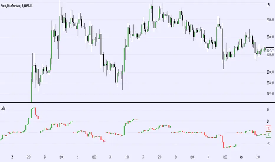
Real Cummulative Delta (New TV Function)Thanks to the new TradingView indicator Up/Down Volume, it is now possible to get accurate information on Agression (market buying vs market selling)
However, as they only provide the value of delta, I've made this indicator to show the cummulative value, in the form of candles.
It is great to detect divergences in the macro and in the micro scale (As in divergences in each candle and divergences in higher or lower tops or bottoms)
Hope you can make good use of it!
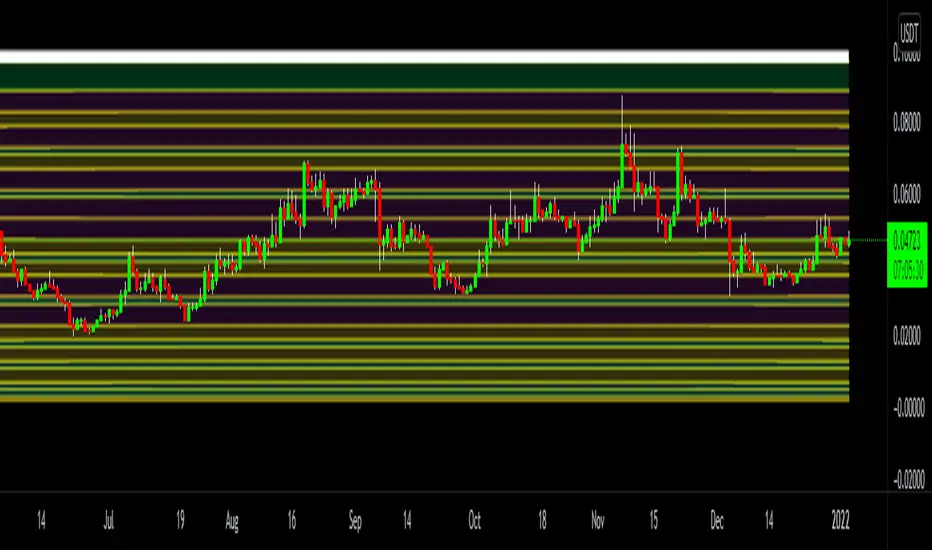
Prime Distance Frame Quant Model for Risk Reward & Pivot PointsIn this script we take all of the prime numbers up to 100 and plot them as olive lines and then consider the distance between two adjacent plots and color code these distances with the fill function. This allows us to find higher and lower prime gaps allowing us to make much more informed decisions on our risk reward for a given trade and the levels where we should consider taking profit.
The Script includes scaling for all assets and is intended to be used for crypto trading.
Terminal : Important U.S Indices Change (%) DataHello.
This script is a simple U.S Indices Data Terminal.
You can also set the period to look back manually in the menu.
In this way, an idea can be obtained about Major U.S Indices.
Features
Value changes on a percentage basis (%)
Recently, due to increasing interest, the NQNACE index has been added.
Index descriptions are printed on the information panel.
Sentiment NYSE ARCA and AMEX indices added.
Indices
SP1! : S&P 500 Futures Index
DJI : Dow Jones Industrial Average Index
NDX : Nasdaq 100 Index
RUT : Russell 2000 Index
NYA : NYSE Composite Index
OSX : PHLX Oil Service Sector Index
HGX : PHLX Housing Sector Index
UTY : PHLX Utility Sector Index
SOX : PHLX Semiconductor Sector Index
SPSIBI : S&P Biotechnology Select Industry Index
XNG : NYSE ARCA Natural Gas Index
SPGSCI : S&P Goldman Sachs Commodity Index
XAU : PHLX Gold and Silver Sector Index
SPSIOP : S&P Oil and Gas Exploration and Production Select Industry Index
GDM : NYSE ARCA Gold Miners Index
DRG : NYSE ARCA Pharmaceutical Index
TOB : NYSE ARCA Tobacco Index
DFI : NYSE ARCA Defense Index
NWX : NYSE ARCA Networking Index
XCI : NYSE ARCA Computer Technology
XOI : AMEX Oil Index
XAL : AMEX Airline Index
NQNACE : Nasdaq Yewno North America Cannabis Economy Index

Terminal : USD Based Stock Markets Change (%)Hello.
This script is a simple USD Based Stock Markets Change (%) Data Terminal.
You can also set the period to look back manually in the menu.
In this way, an idea can be obtained about Countries' Stock Markets.
And you can observe the stock exchanges of relatively positive and negative countries from others.
Features
Value changes on a percentage basis (%)
Stock exchange values are calculated in dollar terms.
Due to the advantage of movement, future data were chosen instead of spot values on the required instruments.
Stock Markets
Usa : S&P 500 Futures
Japan: Nikkei 225 Futures
England: United Kingdom ( FTSE ) 100
Australia: Australia 200
Canada: S&P / TSX Composite
Switzerland: Swiss Market Index
New Zealand: NZX 50 Index
China: SSE Composite (000001)
Denmark: OMX Copenhagen 25 Index
Hong-Kong: Hang Seng Index Futures
India: Nifty 50
Norway: Oslo Bors All Share Index
Russia: MOEX Russia Index
Sweden: OMX Stockholm Index
Singapore: Singapore 30
Turkey: BIST 100
South Africa: South Africa Top 40 Index
Spain: IBEX 35
France: CAC 40
Italy: FTSE MIB Index
Netherlands: Netherlands 25
Germany : DAX
Regards.

General Data TerminalHello.
This script is a simple General Data Terminal.
You can also set the period to look back manually in the menu.
In this way, an idea can be obtained about Global Markets.
Note : TIO = Iron Ore
Regards.

Basic Forex TerminalHello,
This script is a simple Forex terminal.
It serves the same purpose as Heatmaps.
You can also set the period to look back manually in the menu.
Major indicators are taken into account.
In this way, an idea can be obtained about all major and minor currencies.
Best regards.
