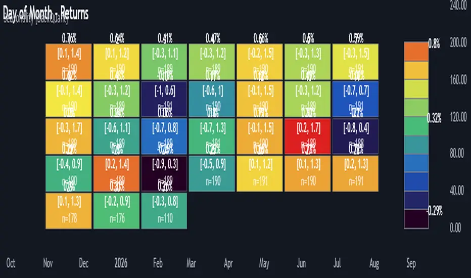
Multi-Mode Seasonality Map [BackQuant]Multi-Mode Seasonality Map
A fast, visual way to expose repeatable calendar patterns in returns, volatility, volume, and range across multiple granularities (Day of Week, Day of Month, Hour of Day, Week of Month). Built for idea generation, regime context, and execution timing.
What is “seasonality” in markets?
Seasonality refers to statistically repeatable patterns tied to the calendar or clock, rather than to price levels. Examples include specific weekdays tending to be stronger, certain hours showing higher realized volatility, or month-end flow boosting volumes. This tool measures those effects directly on your charted symbol.
Why seasonality matters
It’s orthogonal alpha: timing edges independent of price structure that can complement trend, mean reversion, or flow-based setups.
It frames expectations: when a session typically runs hot or cold, you size and pace risk accordingly.
It improves execution: entering during historically favorable windows, avoiding historically noisy windows.
It clarifies context: separating normal “calendar noise” from true anomaly helps avoid overreacting to routine moves.
How traders use seasonality in practice
Timing entries/exits : If Tuesday morning is historically weak for this asset, a mean-reversion buyer may wait for that drift to complete before entering.
Sizing & stops : If 13:00–15:00 shows elevated volatility, widen stops or reduce size to maintain constant risk.
Session playbooks : Build repeatable routines around the hours/days that consistently drive PnL.
Portfolio rotation : Compare seasonal edges across assets to schedule focus and deploy attention where the calendar favors you.
Why Day-of-Week (DOW) can be especially helpful
Flows cluster by weekday (ETF creations/redemptions, options hedging cadence, futures roll patterns, macro data releases), so DOW often encodes a stable micro-structure signal.
Desk behavior and liquidity provision differ by weekday, impacting realized range and slippage.
DOW is simple to operationalize: easy rules like “fade Monday afternoon chop” or “press Thursday trend extension” can be tested and enforced.
What this indicator does
Multi-mode heatmaps : Switch between Day of Week, Day of Month, Hour of Day, Week of Month .
Metric selection : Analyze Returns , Volatility ((high-low)/open), Volume (vs 20-bar average), or Range (vs 20-bar average).
Confidence intervals : Per cell, compute mean, standard deviation, and a z-based CI at your chosen confidence level.
Sample guards : Enforce a minimum sample size so thin data doesn’t mislead.
Readable map : Color palettes, value labels, sample size, and an optional legend for fast interpretation.
Scoreboard : Optional table highlights best/worst DOW and today’s seasonality with CI and a simple “edge” tag.
How it’s calculated (under the hood)
Per bar, compute the chosen metric (return, vol, volume %, or range %) over your lookback window.
Bucket that metric into the active calendar bin (e.g., Tuesday, the 15th, 10:00 hour, or Week-2 of month).
For each bin, accumulate sum , sum of squares , and count , then at render compute mean , std dev , and confidence interval .
Color scale normalizes to the observed min/max of eligible bins (those meeting the minimum sample size).
How to read the heatmap
Color : Greener/warmer typically implies higher mean value for the chosen metric; cooler implies lower.
Value label : The center number is the bin’s mean (e.g., average % return for Tuesdays).
Confidence bracket : Optional “ ” shows the CI for the mean, helping you gauge stability.
n = sample size : More samples = more reliability. Treat small-n bins with skepticism.
Suggested workflows
Pick the lens : Start with Analysis Type = Returns , Heatmap View = Day of Week , lookback ≈ 252 trading days . Note the best/worst weekdays and their CI width.
Sanity-check volatility : Switch to Volatility to see which bins carry the most realized range. Use that to plan stop width and trade pacing.
Check liquidity proxy : Flip to Volume , identify thin vs thick windows. Execute risk in thicker windows to reduce slippage.
Drill to intraday : Use Hour of Day to reveal opening bursts, lunchtime lulls, and closing ramps. Combine with your main strategy to schedule entries.
Calendar nuance : Inspect Week of Month and Day of Month for end-of-month, options-cycle, or data-release effects.
Codify rules : Translate stable edges into rules like “no fresh risk during bottom-quartile hours” or “scale entries during top-quartile hours.”
Parameter guidance
Analysis Period (Days) : 252 for a one-year view. Shorten (100–150) to emphasize the current regime; lengthen (500+) for long-memory effects.
Heatmap View : Start with DOW for robustness, then refine with Hour-of-Day for your execution window.
Confidence Level : 95% is standard; use 90% if you want wider coverage with fewer false “insufficient data” bins.
Min Sample Size : 10–20 helps filter noise. For Hour-of-Day on higher timeframes, consider lowering if your dataset is small.
Color Scheme : Choose a palette with good mid-tone contrast (e.g., Red-Green or Viridis) for quick thresholding.
Interpreting common patterns
Return-positive but low-vol bins : Favorable drift windows for passive adds or tight-stop trend continuation.
Return-flat but high-vol bins : Opportunity for mean reversion or breakout scalping, but manage risk accordingly.
High-volume bins : Better expected execution quality; schedule size here if slippage matters.
Wide CI : Edge is unstable or sample is thin; treat as exploratory until more data accumulates.
Best practices
Revalidate after regime shifts (new macro cycle, liquidity regime change, major exchange microstructure updates).
Use multiple lenses: DOW to find the day, then Hour-of-Day to refine the entry window.
Combine with your core setup signals; treat seasonality as a filter or weight, not a standalone trigger.
Test across assets/timeframes—edges are instrument-specific and may not transfer 1:1.
Limitations & notes
History-dependent: short histories or sparse intraday data reduce reliability.
Not causal: a hot Tuesday doesn’t guarantee future Tuesday strength; treat as probabilistic bias.
Aggregation bias: changing session hours or symbol migrations can distort older samples.
CI is z-approximate: good for fast triage, not a substitute for full hypothesis testing.
Quick setup
Use Returns + Day of Week + 252d to get a clean yearly map of weekday edge.
Flip to Hour of Day on intraday charts to schedule precise entries/exits.
Keep Show Values and Confidence Intervals on while you calibrate; hide later for a clean visual.
The Multi-Mode Seasonality Map helps you convert the calendar from an afterthought into a quantitative edge, surfacing when an asset tends to move, expand, or stay quiet—so you can plan, size, and execute with intent.
Cari dalam skrip untuk "父亲把15万藏被子里被儿子误扔"
X C/P VPDescription
The X C/P VP indicator visualizes intraperiod option flow dynamics for any selected call and put contracts. It plots the volume of both options as overlapping histograms, allowing traders to observe where liquidity and participation are concentrated.
A small dot appears above a bar only when the option’s closing price increases relative to the prior bar, providing an immediate visual cue of upward price pressure within volume spikes.
By combining these two layers—volume intensity and directional confirmation—the indicator makes it easy to spot where the market is actively repricing risk across the call/put structure.
Use Case
Designed for 0DTE and short-dated options, especially index ETFs such as QQQ or SPY.
Helps traders compare call vs. put participation to gauge sentiment skew and intraday balance.
Useful for monitoring volume surges tied to delta hedging, gamma shifts, or option repricing following volatility or directional moves.
Can be applied on 1-minute to 15-minute timeframes to observe how option volume evolves through key market sessions (e.g., open, midday, close).
Dots highlight periods where premium expansion accompanies increased volume—often an early sign of momentum or positioning bias.
Summary
X C/P VP serves as a lightweight, visually intuitive tool to read the rhythm of call and put activity intraday—offering an at-a-glance pulse of which side of the options market is taking control.

USD Session 8FX - LDN & NY (TF-invariant, Live + Table)What changed
Flexible session window
Removed the old fixed NY end-time selector.
Added new inputs so you can pick start time and length:
London: ldnStartSel (default 08:00) and ldnLenSel with options 45/60/90 minutes.
New York: nyStartSel (default 15:30) and nyLenSel with options 45/60/90 minutes.
The session string used by time(refTF, sess, tz) is now built dynamically as "HHMM-HHMM" from start + length (e.g., 1530-1630).
The label shown in the table (winTxt) auto-formats to HH:MM–HH:MM.
New time helpers
addMinutesHHMM() computes the end time from a "HHMM" start plus a minute length.
makeSess() produces the session string "HHMM-HHMM".
prettySess() converts "HHMM-HHMM" → "HH:MM-HH:MM".
(Kept on one line to avoid the “end of line without line continuation” error.)
Stability & UI fixes
Main table now uses table.new(f_pos(tablePos), ...) directly (no undeclared pos variable).
Trade Gate panel uses a properly initialized gatePosEnum before table.new(...) (fixes “Undeclared identifier”).
Minor cleanups; no logic changes.
What did NOT change
Scoring logic: returns → optional ATR normalization → weights → anti-USD vs USD-base averages → final score.
Thresholds: minAbsScore and live intrath alerts are unchanged.
VWAP Gate logic is the same (price vs VWAP consistency depending on USD Strong/Weak).
Freeze/Lock of values at session end is unchanged.
Alerts (session close bias, live threshold cross, and “Entry hint”) are unchanged.
Why this helps (practical impact)
Longer windows (e.g., NY 60/90, LDN 60/90) usually make the score more robust, filtering noise and reducing false signals—at the cost of a slightly slower signal.
You can now A/B test:
London: 45 vs 60 vs 90
New York: 45 vs 60 vs 90
without touching anything else; the indicator adapts automatically.
How to use
Choose Session (London / New York).
Set the start and length for that session.
The background highlight, the winTxt, and the entry/exit logic all follow the dynamic window.
Quick tips to reduce false signals
Try NY 60 or NY 90 and LDN 60 when volatility is choppy.
Keep ATR normalization ON (useATRnorm = true) for more comparable returns.
Consider raising minAbsScore slightly (e.g., from 0.12 → 0.15–0.20) if you still see noise.
Use the VWAP Gate panel: only act when Bias OK and at least one of the Top-3 pairs shows VWAP OK.
If you want, I can add quick presets (buttons) to jump between LDN 45/60/90 and NY 45/60/90, or plot two Scores side by side for direct comparison.

Lateral Market DetectorOverview
The Lateral Market Detector is a TradingView indicator designed to identify and highlight range-bound market conditions (sideways movement) where price oscillates between defined support and resistance levels with minimal overall movement.
How It Works
The indicator analyzes price action using a dynamic range detection algorithm:
Range Calculation: Examines the last N candlesticks (default 50, adjustable 20-200) and calculates the difference between the highest high and lowest low within this period.
Laterality Detection: Compares the calculated range against a configurable tolerance threshold (in pips). If the range is smaller than the tolerance, the market is identified as laterally moving.
Confirmation Logic: Counts consecutive candlesticks that remain within the detected range. The indicator only confirms a lateral condition when the minimum number of consecutive candlesticks has been reached (default 15).
Visual Representation: Once confirmed, displays a colored rectangle (box) spanning from the range's start point to the current bar, with horizontal dashed lines marking the high and low levels.
Dynamic Update: Continuously updates the rectangle as new candlesticks form, adjusting the top and bottom boundaries if price remains within the lateral zone.
Key Features
Multi-Timeframe Optimization
Automatic timeframe adaptation using square root scaling
When enabled, parameters adjust proportionally based on the current timeframe (M1, M5, M15, M30, H1, D1, W1, MN)
Prevents the need for manual parameter adjustments across different timeframes
Formula: Adjusted_Tolerance = Base_Tolerance × √(Timeframe_Multiplier)
Customizable Parameters
Tolerance Pip (M1): Sets the maximum range width to identify laterality
Minimum Candlesticks: Minimum consecutive candles required to confirm a lateral zone
Candlesticks to Analyze: Lookback period for range calculation
Breakout Sensitivity: Controls the threshold for identifying range breakouts
Full Visual Customization
Rectangle color and transparency
High/Low line color and thickness
Automatic status display showing current timeframe, lateral confirmation, and active parameters
Use Cases
Range Trading: Identify optimal entry and exit points at support/resistance
Breakout Trading: Visual confirmation before entering breakout trades
Trend Analysis: Distinguish between trending and consolidating markets
Risk Management: Define clear stop-loss levels based on range boundaries
Technical Specifications
Indicator Type: Overlay
Maximum Boxes: 100 (prevents performance degradation)
Supported Assets: Forex, CFDs, Stocks, Cryptocurrencies
Pine Script Version: v5
Chart Display: Real-time updates on each new candlestick

RightFlow Universal Volume Profile - Any Market Any TimeframeSummary in one paragraph
RightFlow is a right anchored microstructure volume profile for stocks, futures, FX, and liquid crypto on intraday and daily timeframes. It acts only when several conditions align inside a session window and presents the result as a compact right side profile with value area, POC, a bull bear mix by price bin, and a HUD of profile VWAP and pressure shares. It is original because it distributes each bar’s weight into multiple mid price slices, blends bull bear pressure per bin with a CLV based split, and grows the profile to the right so price action stays readable. Add to a clean chart, read the table, and use the visuals. For conservative workflows read on bar close.
Scope and intent
• Markets. Major FX pairs, index futures, large cap equities and ETFs, liquid crypto.
• Timeframes. One minute to daily.
• Default demo used in the publication. SPY on 15 minute.
• Purpose. See where participation concentrates, which side dominated by price level, and how far price sits from VA and POC.
Originality and usefulness
• Unique fusion. Right anchored growth plus per bar slicing and CLV split, with weight modes Raw, Notional, and DeltaProxy.
• Failure mode addressed. False reads from single bar direction and coarse binning.
• Testability. All parts sit in Inputs and the HUD.
• Portable yardstick. Value Area percent and POC are universal across symbols.
• Protected scripts. Not applicable. Method and use are fully disclosed.
Method overview in plain language
Pick a scope Rolling or Today or This Week. Define a window and number of price bins. For each bar, split its range into small slices, assign each slice a weight from the selected mode, and split that weight by CLV or by bar direction. Accumulate totals per bin. Find the bin with the highest total as POC. Expand left and right until the chosen share of total volume is covered to form the value area. Compute profile VWAP for all, buyers, and sellers and show them with pressure shares.
Base measures
Range basis. High minus low and mid price samples across the bar window.
Return basis. Not used. VWAP trio is price weighted by weights.
Components
• RightFlow Bins. Price histogram that grows to the right.
• Bull Bear Split. CLV based 0 to 1 share or pure bar direction.
• Weight Mode. Raw volume, notional volume times close, or DeltaProxy focus.
• Value Area Engine. POC then outward expansion to target share.
• HUD. Profile VWAP, Buy and Sell percent, winner delta, split and weight mode.
• Session windows optional. Scope resets on day or week.
Fusion rule
Color of each bin is the convex blend of bull and bear shares. Value area shading is lighter inside and darker outside.
Signal rule
This is context, not a trade signal. A strong separation between buy and sell percent with price holding inside VA often confirms balance. Price outside VA with skewed pressure often marks initiative moves.
What you will see on the chart
• Right side bins with blended colors.
• A POC line across the profile width.
• Labels for POC, VAH, and VAL.
• A compact HUD table in the top right.
Table fields and quick reading guide
• VWAP. Profile VWAP.
• Buy and Sell. Pressure shares in percent.
• Delta Winner. Winner side and margin in percent.
• Split and Weight. The active modes.
Reading tip. When Session scope is Today or This Week and Buy minus Sell is clearly positive or negative, that side often controls the day’s narrative.
Inputs with guidance
Setup
• Profile scope. Rolling or session reset. Rolling uses window bars.
• Rolling window bars. Typical 100 to 300. Larger is smoother.
Binning
• Price bins. Typical 32 to 128. More bins increase detail.
• Slices per bar. Typical 3 to 7. Raising it smooths distribution.
Weighting
• Weight mode. Raw, Notional, DeltaProxy. Notional emphasizes expensive prints.
• Bull Bear split. CLV or BarDir. CLV is more nuanced.
• Value Area percent. Typical 68 to 75.
View
• Profile width in bars, color split toggle, value area shading, opacities, POC line, VA labels.
Usage recipes
Intraday trend focus
• Scope Today, bins 64, slices 5, Value Area 70.
• Split CLV, Weight Notional.
Intraday mean reversion
• Scope Today, bins 96, Value Area 75.
• Watch fades back to POC after initiative pushes.
Swing continuation
• Scope Rolling 200 bars, bins 48.
• Use Buy Sell skew with price relative to VA.
Realism and responsible publication
No performance claims. Shapes can move while a bar forms and settle on close. Education only.
Honest limitations and failure modes
Thin liquidity and data gaps can distort bin weights. Very quiet regimes reduce contrast. Session time is the chart venue time.
Open source reuse and credits
None.
Legal
Education and research only. Not investment advice. Test on history and simulation before live use.

Weighted Moving Average (WMA)This implementation uses O(1) algorithm that eliminates the need to loop through all period values on each bar. It also generates valid WMA values from the first bar and is not returning NA when number of bars is less than period.
## Overview and Purpose
The Weighted Moving Average (WMA) is a technical indicator that applies progressively increasing weights to more recent price data. Emerging in the early 1950s during the formative years of technical analysis, WMA gained significant adoption among professional traders through the 1970s as computational methods became more accessible. The approach was formalized in Robert Colby's 1988 "Encyclopedia of Technical Market Indicators," establishing it as a staple in technical analysis software. Unlike the Simple Moving Average (SMA) which gives equal weight to all prices, WMA assigns greater importance to recent prices, creating a more responsive indicator that reacts faster to price changes while still providing effective noise filtering.
## Core Concepts
* **Linear weighting:** WMA applies progressively increasing weights to more recent price data, creating a recency bias that improves responsiveness
* **Market application:** Particularly effective for identifying trend changes earlier than SMA while maintaining better noise filtering than faster-responding averages like EMA
* **Timeframe flexibility:** Works effectively across all timeframes, with appropriate period adjustments for different trading horizons
The core innovation of WMA is its linear weighting scheme, which strikes a balance between the equal-weight approach of SMA and the exponential decay of EMA. This creates an intuitive and effective compromise that prioritizes recent data while maintaining a finite lookback period, making it particularly valuable for traders seeking to reduce lag without excessive sensitivity to price fluctuations.
## Common Settings and Parameters
| Parameter | Default | Function | When to Adjust |
|-----------|---------|----------|---------------|
| Length | 14 | Controls the lookback period | Increase for smoother signals in volatile markets, decrease for responsiveness |
| Source | close | Price data used for calculation | Consider using hlc3 for a more balanced price representation |
**Pro Tip:** For most trading applications, using a WMA with period N provides better responsiveness than an SMA with the same period, while generating fewer whipsaws than an EMA with comparable responsiveness.
## Calculation and Mathematical Foundation
**Simplified explanation:**
WMA calculates a weighted average of prices where the most recent price receives the highest weight, and each progressively older price receives one unit less weight. For example, in a 5-period WMA, the most recent price gets a weight of 5, the next most recent a weight of 4, and so on, with the oldest price getting a weight of 1.
**Technical formula:**
```
WMA = (P₁ × w₁ + P₂ × w₂ + ... + Pₙ × wₙ) / (w₁ + w₂ + ... + wₙ)
```
Where:
- Linear weights: most recent value has weight = n, second most recent has weight = n-1, etc.
- The sum of weights for a period n is calculated as: n(n+1)/2
- For example, for a 5-period WMA, the sum of weights is 5(5+1)/2 = 15
**O(1) Optimization - Dual Running Sums:**
The key insight is maintaining two running sums:
1. **Unweighted sum (S)**: Simple sum of all values in the window
2. **Weighted sum (W)**: Sum of all weighted values
The recurrence relation for a full window is:
```
W_new = W_old - S_old + (n × P_new)
```
This works because when all weights decrement by 1 (as the window slides), it's mathematically equivalent to subtracting the entire unweighted sum. The implementation:
- **During warmup**: Accumulates both sums as the window fills, computing denominator each bar
- **After warmup**: Uses cached denominator (constant at n(n+1)/2), updates both sums in constant time
- **Performance**: ~8 operations per bar regardless of period, vs ~100+ for naive O(n) implementation
> 🔍 **Technical Note:** Unlike EMA which theoretically considers all historical data (with diminishing influence), WMA has a finite memory, completely dropping prices that fall outside its lookback window. This creates a cleaner break from outdated market conditions. The O(1) optimization achieves 12-25x speedup over naive implementations while maintaining exact mathematical equivalence.
## Interpretation Details
WMA can be used in various trading strategies:
* **Trend identification:** The direction of WMA indicates the prevailing trend with greater responsiveness than SMA
* **Signal generation:** Crossovers between price and WMA generate trade signals earlier than with SMA
* **Support/resistance levels:** WMA can act as dynamic support during uptrends and resistance during downtrends
* **Moving average crossovers:** When a shorter-period WMA crosses above a longer-period WMA, it signals a potential uptrend (and vice versa)
* **Trend strength assessment:** Distance between price and WMA can indicate trend strength
## Limitations and Considerations
* **Market conditions:** Still suboptimal in highly volatile or sideways markets where enhanced responsiveness may generate false signals
* **Lag factor:** While less than SMA, still introduces some lag in signal generation
* **Abrupt window exit:** The oldest price suddenly drops out of calculation when leaving the window, potentially causing small jumps
* **Step changes:** Linear weighting creates discrete steps in influence rather than a smooth decay
* **Complementary tools:** Best used with volume indicators and momentum oscillators for confirmation
## References
* Colby, Robert W. "The Encyclopedia of Technical Market Indicators." McGraw-Hill, 2002
* Murphy, John J. "Technical Analysis of the Financial Markets." New York Institute of Finance, 1999
* Kaufman, Perry J. "Trading Systems and Methods." Wiley, 2013
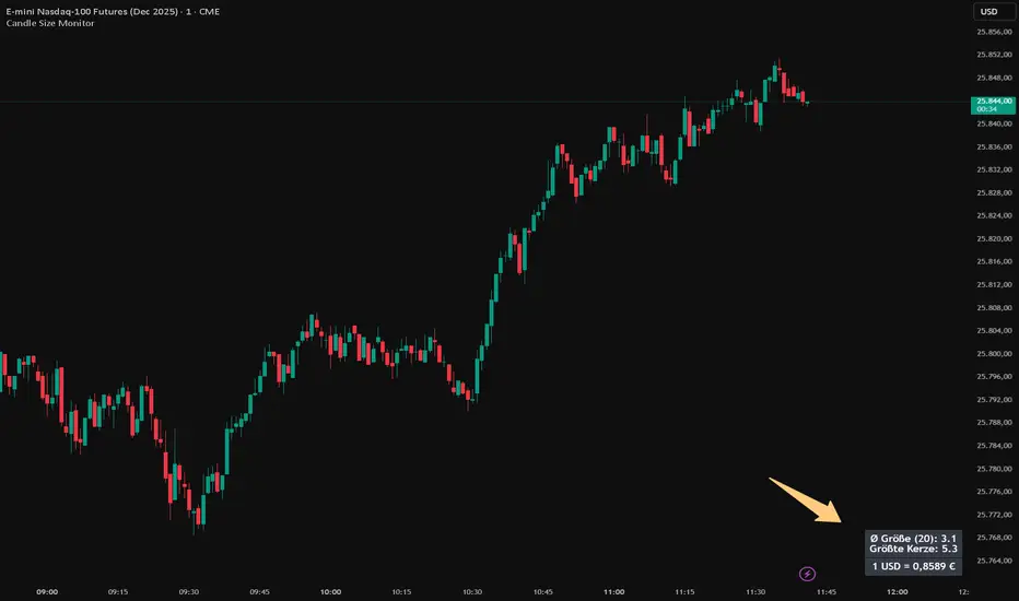
Candle Size MonitorCandle Size Monitor – Description
Update 27.10.25
Objective Volatility Assessment
The Candle Size Monitor helps traders assess actual market movement—regardless of whether candles appear visually large or small on the chart. It supports evaluating whether your planned trade structure (e.g., stop-loss, take-profit) aligns with current volatility.
Key Features
Volatility Analysis:
Calculates the average candle size (difference between high and low) over a user-defined number of candles.
Identifies the largest candle in the selected period.
Displays results in a compact table on the chart.
Exchange Rate Integration (optional):
Shows the current USD-EUR exchange rate (formatted with German-style comma and four decimal places).
Useful for traders in USD-denominated markets who apply EUR-based risk management rules.
Customizable Display:
Text Size: Small, medium, or large.
Colors: Customizable text and background colors.
Table Position: Top/bottom left/right.
Number of Candles: User-defined (default: 20).
Dynamic Updates:
The table updates with each new bar.
The exchange rate is fetched in real-time from OANDA:EURUSD.
Settings and Translations
Settings
Anzahl Kerzen → Number of Candles (Number of candles for calculation, default: 20).
Textgröße → Text Size (Text size in the table: small, medium, large).
Textfarbe → Text Color (Text color, default: white).
Hintergrundfarbe → Background Color (Background color of the table, default: black).
Position → Position (Table position: Top Left, Top Right, Bottom Left, Bottom Right).
Wechselkurs anzeigen (USD → EUR) → Show Exchange Rate (USD → EUR) (Option to display the exchange rate).
Table Contents and Translations
The table displays the following information (with German formatting):
Ø Größe (N):
English: "Avg Size (N): " (Average candle size over the last N candles).
Example: "Ø Größe (20): 15,3" → "Avg Size (20): 15.3".
Größte Kerze:
English: "Largest Candle: " (Largest candle size in the selected period).
Example: "Größte Kerze: 42,7" → "Largest Candle: 42.7".
1 USD = € (only if enabled)
English: "1 USD = EUR" (Current USD-EUR exchange rate, formatted with a comma).
Example: "1 USD = 0,9234 €" → "1 USD = 0.9234 EUR".
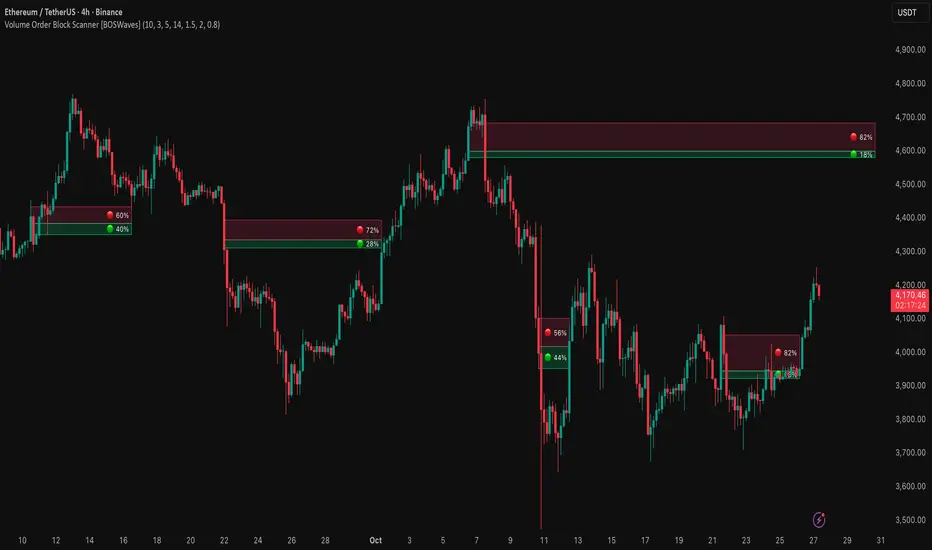
Volume Order Block Scanner [BOSWaves]Volume Order Block Scanner - Dynamic Detection of High-Volume Supply and Demand Zones
Overview
The Volume Order Block Scanner introduces a refined approach to institutional zone mapping, combining volume-weighted order flow, structural displacement, and ATR-based proportionality to identify regions of aggressive participation from large entities.
Unlike static zone mapping or simplistic body-size filters, this framework dynamically evaluates each candle through a multi-layer model of relative volume, candle structure, and volatility context to isolate genuine order block formations while filtering out market noise.
Each identified zone represents a potential institutional footprint, defined by significant volume surges and efficient body-to-ATR relationships that indicate purposeful positioning. Once mapped, each order block is dynamically adjusted for volatility and tracked throughout its lifecycle - from creation to mitigation to potential invalidation - producing an evolving liquidity map that adapts with price.
This adaptive behavior allows traders to visualize where liquidity was absorbed and where it remains unfilled, revealing the structural foundation of institutional intent across timeframes.
Theoretical Foundation
At its core, the Volume Order Block Scanner is built on the interaction between volume displacement and structural imbalance. Traditional order block systems often rely on fixed candle formations or simple engulfing logic, neglecting the fundamental driver of institutional activity: volume concentration relative to volatility.
This framework redefines that approach. Each candle is filtered through two comparative ratios:
Relative Volume Ratio (RVR) - the candle’s volume compared to its rolling average, confirming genuine transactional surges.
Body-ATR Ratio (BAR) - a measure of displacement efficiency relative to recent volatility, ensuring structural strength.
Only when both conditions align is an order block validated, marking a displacement event significant enough to create a lasting imbalance.
By embedding this logic within a volatility-adjusted environment, the system maintains scalability across asset classes and volatility regimes - equally effective in crypto, forex, or index markets.
How It Works
The Volume Order Block Scanner operates through a structured multi-stage process:
Displacement Detection - Identifies candles whose body and volume exceed dynamic thresholds derived from ATR and rolling volume averages. These represent the origin points of institutional aggression.
Zone Construction - Each qualified candle generates an order block with ATR-proportional dimensions to ensure consistency across instruments and timeframes. The zone includes two regions: Body Zone (the precise initiation point of displacement) and Wick Imbalance (the residual inefficiency representing unfilled liquidity).
Lifecycle Tracking - Each zone is continuously monitored for market interaction. Reactions within a defined window are classified as respected, mitigated, or invalidated, giving traders a data-driven sense of ongoing institutional relevance.
Volume Confirmation Layer - Reinforces signal integrity by ensuring that all detected blocks correspond with meaningful increases in transactional activity.
Temporal Decay Control - Zones that remain untested beyond a set period gradually lose visual and analytical weight, maintaining chart clarity and contextual precision.
Interpretation
The Volume Order Block Scanner visualizes how institutional participants interact with the market through zones of accumulation and distribution.
Bullish order blocks denote demand imbalances where price displaced upward under high volume; bearish order blocks signify supply regions formed by concentrated selling pressure.
Price revisiting these areas often reflects institutional re-entry or liquidity rebalancing, offering actionable insights for both continuation and reversal scenarios.
By continuously monitoring interaction and expiry, the framework enables traders to distinguish between active institutional footprints and historical liquidity artifacts.
Strategy Integration
The Volume Order Block Scanner integrates naturally into advanced structural and order-flow methodologies:
Liquidity Mapping : Identify high-volume regions that are likely to influence future price reactions.
Break-of-Structure Confirmation : Validate BOS and CHOCH signals through aligned order block behavior.
Volume Confluence : Combine with BOSWaves volume or momentum indicators to confirm real institutional intent.
Smart-Money Frameworks : Utilize order block retests as precision entry zones within SMC-based setups.
Trend Continuation : Filter zones in line with higher-timeframe bias to maintain directional integrity.
Technical Implementation Details
Core Engine : Dual-filter mechanism using Relative Volume Ratio (RVR) and Body-ATR Ratio (BAR).
Volatility Framework : ATR-based scaling for cross-asset proportionality.
Zone Composition : Body and wick regions plotted independently for visual clarity of imbalance.
Lifecycle Logic : Real-time monitoring of reaction, mitigation, and invalidation states.
Directional Coloring : Distinct bullish and bearish shading with adjustable transparency.
Computation Efficiency : Lightweight structure suitable for multi-timeframe or multi-asset environments.
Optimal Application Parameters
Timeframe Guidance:
5m - 15m : Reactive intraday zones for short-term liquidity engagement.
1H - 4H : Medium-term structures for swing or intraday trend mapping.
Daily - Weekly : Macro accumulation and distribution footprints.
Suggested Configuration:
Relative Volume Threshold : 1.5× - 2.0× average volume.
Body-ATR Threshold : 0.8× - 1.2× for valid displacement.
Zone Expiry : 5 - 10 bars for intraday use, 15 - 30 for swing/macro contexts.
Parameter optimization should be asset-specific, tuned to volatility conditions and liquidity depth.
Performance Characteristics
High Effectiveness:
Markets exhibiting clear displacement and directional flow.
Environments with consistent volume expansion and liquidity inefficiencies.
Reduced Effectiveness:
Range-bound markets with frequent false impulses.
Low-volume sessions lacking institutional participation.
Integration Guidelines
Confluence Framework : Pair with structure-based BOS or liquidity tools for validation.
Risk Management : Treat active order blocks as contextual areas of interest, not guaranteed reversal points.
Multi-Timeframe Logic : Derive bias from higher-timeframe blocks and execute from refined lower-timeframe structures.
Volume Verification : Confirm each reaction with concurrent volume acceleration to avoid false liquidity cues.
Disclaimer
The Volume Order Block Scanner is a quantitative mapping framework designed for professional traders and analysts. It is not a predictive or guaranteed system of profit.
Performance depends on correct configuration, market conditions, and disciplined risk management. BOSWaves recommends using this indicator as part of a comprehensive analytical process - integrating structural, volume, and liquidity context for accurate interpretation.
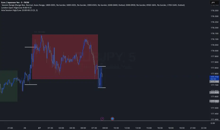
Asia Session High/Low 23:00-00:15This indicator shows highs and lows 1 hour before Asia session and the first 15min of Asia session.
Flux AI PullBack System (Hybrid Pro)Flux AI PullBack System (Hybrid Pro)
//Session-Aware | Adaptive Confluence | Grace Confirm Logic//
Overview:
The Flux AI PullBack System (Hybrid Pro v5) is an adaptive, session-aware pullback indicator designed to identify high-probability continuation setups within trending markets. It automatically adjusts between “Classic” and “Enhanced” logic modes based on volatility, volume, and ATR slope, allowing it to perform seamlessly across different market sessions (Asian, London, and New York).
Core Features:
Hybrid Auto Mode — Dynamically switches between Classic (fast-moving) and Enhanced (strict) modes.
Session-Aware Context — Optimized for intraday trading in ES, NQ, and SPY.
Grace Confirmation Logic — Validates pullbacks with a follow-through condition to reduce noise.
Adaptive EMA Zone (38/62) — Highlights pullback areas with dynamic aqua fill and transparency linked to trend strength.
Noise Suppression Filter — Prevents false pullbacks during EMA crossovers or unstable transitions.
Weighted Confluence Model — Combines trend, ATR, volume, and swing structure for confirmation strength.
Pine v6 Compliant Alerts — Constant-string safe, ready for webhooks and automation.
Visual Elements:
Aqua EMA Zone: Displays the “breathing” pullback band (tightens during volatility spikes).
PB↑ / PB↓ Markers: Confirmed pullbacks with subtle transparency and fixed label size.
Bar Highlights: Yellow for pullbacks; ice-blue for confirmed continuation.
Use Cases
Perfect for:
Intraday trend traders
0DTE SPX / ES scalpers
Futures traders (NQ, MNQ, MES)
Algorithmic strategy builders using webhooks
Recommended Timeframes:
1–15 minute charts (scalping / intraday)
Higher timeframes for swing confirmations.
Attribution:
This open-source script was inspired by Chris Moody’s “CM Slingshot System” and JustUncleL’s Pullback Tools, but it was built from scratch using AI-assisted code refinement (ChatGPT).
All logic and enhancements are original, not derived from proprietary software.
License: MIT (Open Source)
© 2025 Ken Anderson — You may modify, use, or redistribute with credit.
Keywords:
Pullback, Reversal, AI Trading, EMA Zone, Session Aware, Futures Trading, SPX, ES, NQ, ATR Filter, Volume Confirmation, Flux System, Pine Script v6, Non-Repainting, Adaptive Trading Indicator.
PDB - RSI Based Buy/Sell signals with 4 MARSI Based Buy/Sell Signals on Price chart + 4 MA System
This indicator plots RSI-based Buy & Sell signals directly on the price chart , combined with a 4-Moving-Average trend filter (20/50/100/200) for higher accuracy and cleaner trade timing.
The signal triggers when RSI reaches user-defined overbought/oversold levels, but unlike a standard RSI, this version plots the signals **on the chart**, not in the RSI window — making entries and exits easier to see in real time.
RSI Levels Are Fully Customizable
The default RSI thresholds are 30 (oversold) and 70 (overbought).
However, you can adjust these to fit your trading style. For example:
> When day trading on the 5–15 min timeframe, I personally use 35 (oversold) and 75 (overbought) to catch moves earlier.
> The example shown in the preview image uses 10-minute timeframe settings.
You can change the RSI levels to trigger signals from **any value you choose**, allowing you to tailor the indicator to scalping, day trading, or swing trading.
4 Moving Averages Included:
20, 50, 100, 200 MAs act as dynamic trend filters so you can:
✔ trade signals only in the direction of trend
✔ avoid false reversals
✔ identify momentum shifts more clearly
Works on all markets and timeframes — crypto, stocks, FX, indices.
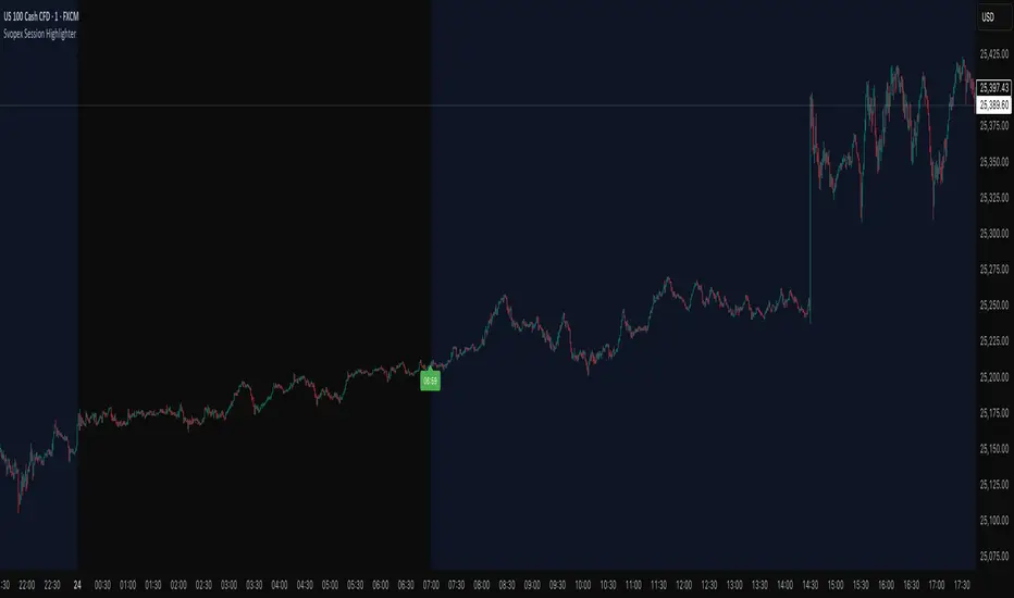
Svopex Session Highlighter# Session Highlighter
## Description
**Session Highlighter** is a powerful Pine Script indicator designed to visually identify and mark specific trading hours on your chart. This tool helps traders focus on their preferred trading sessions by highlighting the background during active hours and marking the session start with customizable visual markers.
## Key Features
- **📊 Session Background Highlighting**: Automatically shades the chart background during your defined trading hours (default: 7:00 - 23:00)
- **🎯 Smart Session Start Marker**: Places a marker on the last candle before session start, intelligently adapting to your timeframe:
- 1 Hour chart: Marker at 6:00
- 15 Minute chart: Marker at 6:45
- 5 Minute chart: Marker at 6:55
- 1 Minute chart: Marker at 6:59
- **🌍 Timezone Support**: Choose from multiple timezones (Europe/Prague, Europe/London, America/New_York, UTC)
- **🎨 5 Marker Styles**: Customize your session start indicator:
- Triangle
- Circle
- Diamond
- Label with time text
- Vertical line
- **⚙️ Fully Customizable**: Adjust start/end hours, timezone, and marker style through simple settings
## Settings
- **Start Hour**: Set your session start time (0-23)
- **End Hour**: Set your session end time (0-23)
- **Timezone**: Select your trading timezone
- **Marker Style**: Choose your preferred visual marker
## Use Cases
- Identify London/New York trading sessions
- Mark Asian session hours
- Highlight your personal trading windows
- Avoid trading during off-hours
- Perfect for day traders and scalpers
## Installation
1. Copy the Pine Script code
2. Open TradingView Pine Editor
3. Paste the code and click "Add to Chart"
4. Configure settings to match your trading schedule
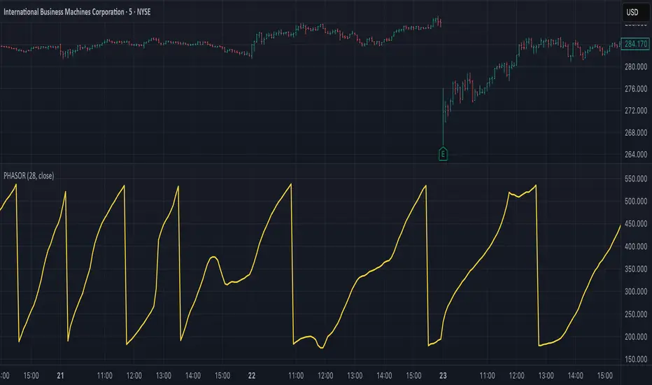
Ehlers Phasor Analysis (PHASOR)# PHASOR: Phasor Analysis (Ehlers)
## Overview and Purpose
The Phasor Analysis indicator, developed by John Ehlers, represents an advanced cycle analysis tool that identifies the phase of the dominant cycle component in a time series through complex signal processing techniques. This sophisticated indicator uses correlation-based methods to determine the real and imaginary components of the signal, converting them to a continuous phase angle that reveals market cycle progression. Unlike traditional oscillators, the Phasor provides unwrapped phase measurements that accumulate continuously, offering unique insights into market timing and cycle behavior.
## Core Concepts
* **Complex Signal Analysis** — Uses real and imaginary components to determine cycle phase
* **Correlation-Based Detection** — Employs Ehlers' correlation method for robust phase estimation
* **Unwrapped Phase Tracking** — Provides continuous phase accumulation without discontinuities
* **Anti-Regression Logic** — Prevents phase angle from moving backward under specific conditions
Market Applications:
* **Cycle Timing** — Precise identification of cycle peaks and troughs
* **Market Regime Analysis** — Distinguishes between trending and cycling market conditions
* **Turning Point Detection** — Advanced warning system for potential market reversals
## Common Settings and Parameters
| Parameter | Default | Function | When to Adjust |
|-----------|---------|----------|----------------|
| Period | 28 | Fixed cycle period for correlation analysis | Match to expected dominant cycle length |
| Source | Close | Price series for phase calculation | Use typical price or other smoothed series |
| Show Derived Period | false | Display calculated period from phase rate | Enable for adaptive period analysis |
| Show Trend State | false | Display trend/cycle state variable | Enable for regime identification |
## Calculation and Mathematical Foundation
**Technical Formula:**
**Stage 1: Correlation Analysis**
For period $n$ and source $x_t$:
Real component correlation with cosine wave:
$$R = \frac{n \sum x_t \cos\left(\frac{2\pi t}{n}\right) - \sum x_t \sum \cos\left(\frac{2\pi t}{n}\right)}{\sqrt{D_{cos}}}$$
Imaginary component correlation with negative sine wave:
$$I = \frac{n \sum x_t \left(-\sin\left(\frac{2\pi t}{n}\right)\right) - \sum x_t \sum \left(-\sin\left(\frac{2\pi t}{n}\right)\right)}{\sqrt{D_{sin}}}$$
where $D_{cos}$ and $D_{sin}$ are normalization denominators.
**Stage 2: Phase Angle Conversion**
$$\theta_{raw} = \begin{cases}
90° - \arctan\left(\frac{I}{R}\right) \cdot \frac{180°}{\pi} & \text{if } R \neq 0 \\
0° & \text{if } R = 0, I > 0 \\
180° & \text{if } R = 0, I \leq 0
\end{cases}$$
**Stage 3: Phase Unwrapping**
$$\theta_{unwrapped}(t) = \theta_{unwrapped}(t-1) + \Delta\theta$$
where $\Delta\theta$ is the normalized phase difference.
**Stage 4: Ehlers' Anti-Regression Condition**
$$\theta_{final}(t) = \begin{cases}
\theta_{final}(t-1) & \text{if regression conditions met} \\
\theta_{unwrapped}(t) & \text{otherwise}
\end{cases}$$
**Derived Calculations:**
Derived Period: $P_{derived} = \frac{360°}{\Delta\theta_{final}}$ (clamped to )
Trend State:
$$S_{trend} = \begin{cases}
1 & \text{if } \Delta\theta \leq 6° \text{ and } |\theta| \geq 90° \\
-1 & \text{if } \Delta\theta \leq 6° \text{ and } |\theta| < 90° \\
0 & \text{if } \Delta\theta > 6°
\end{cases}$$
> 🔍 **Technical Note:** The correlation-based approach provides robust phase estimation even in noisy market conditions, while the unwrapping mechanism ensures continuous phase tracking across cycle boundaries.
## Interpretation Details
* **Phasor Angle (Primary Output):**
- **+90°**: Potential cycle peak region
- **0°**: Mid-cycle ascending phase
- **-90°**: Potential cycle trough region
- **±180°**: Mid-cycle descending phase
* **Phase Progression:**
- Continuous upward movement → Normal cycle progression
- Phase stalling → Potential cycle extension or trend development
- Rapid phase changes → Cycle compression or volatility spike
* **Derived Period Analysis:**
- Period < 10 → High-frequency cycle dominance
- Period 15-40 → Typical swing trading cycles
- Period > 50 → Trending market conditions
* **Trend State Variable:**
- **+1**: Long trend conditions (slow phase change in extreme zones)
- **-1**: Short trend or consolidation (slow phase change in neutral zones)
- **0**: Active cycling (normal phase change rate)
## Applications
* **Cycle-Based Trading:**
- Enter long positions near -90° crossings (cycle troughs)
- Enter short positions near +90° crossings (cycle peaks)
- Exit positions during mid-cycle phases (0°, ±180°)
* **Market Timing:**
- Use phase acceleration for early trend detection
- Monitor derived period for cycle length changes
- Combine with trend state for regime-appropriate strategies
* **Risk Management:**
- Adjust position sizes based on cycle clarity (derived period stability)
- Implement different risk parameters for trending vs. cycling regimes
- Use phase velocity for stop-loss placement timing
## Limitations and Considerations
* **Parameter Sensitivity:**
- Fixed period assumption may not match actual market cycles
- Requires cycle period optimization for different markets and timeframes
- Performance degrades when multiple cycles interfere
* **Computational Complexity:**
- Correlation calculations over full period windows
- Multiple mathematical transformations increase processing requirements
- Real-time implementation requires efficient algorithms
* **Market Conditions:**
- Most effective in markets with clear cyclical behavior
- May provide false signals during strong trending periods
- Requires sufficient historical data for correlation analysis
Complementary Indicators:
* MESA Adaptive Moving Average (cycle-based smoothing)
* Dominant Cycle Period indicators
* Detrended Price Oscillator (cycle identification)
## References
1. Ehlers, J.F. "Cycle Analytics for Traders." Wiley, 2013.
2. Ehlers, J.F. "Cybernetic Analysis for Stocks and Futures." Wiley, 2004.
Ehlers Autocorrelation Periodogram (EACP)# EACP: Ehlers Autocorrelation Periodogram
## Overview and Purpose
Developed by John F. Ehlers (Technical Analysis of Stocks & Commodities, Sep 2016), the Ehlers Autocorrelation Periodogram (EACP) estimates the dominant market cycle by projecting normalized autocorrelation coefficients onto Fourier basis functions. The indicator blends a roofing filter (high-pass + Super Smoother) with a compact periodogram, yielding low-latency dominant cycle detection suitable for adaptive trading systems. Compared with Hilbert-based methods, the autocorrelation approach resists aliasing and maintains stability in noisy price data.
EACP answers a central question in cycle analysis: “What period currently dominates the market?” It prioritizes spectral power concentration, enabling downstream tools (adaptive moving averages, oscillators) to adjust responsively without the lag present in sliding-window techniques.
## Core Concepts
* **Roofing Filter:** High-pass plus Super Smoother combination removes low-frequency drift while limiting aliasing.
* **Pearson Autocorrelation:** Computes normalized lag correlation to remove amplitude bias.
* **Fourier Projection:** Sums cosine and sine terms of autocorrelation to approximate spectral energy.
* **Gain Normalization:** Automatic gain control prevents stale peaks from dominating power estimates.
* **Warmup Compensation:** Exponential correction guarantees valid output from the very first bar.
## Implementation Notes
**This is not a strict implementation of the TASC September 2016 specification.** It is a more advanced evolution combining the core 2016 concept with techniques Ehlers introduced later. The fundamental Wiener-Khinchin theorem (power spectral density = Fourier transform of autocorrelation) is correctly implemented, but key implementation details differ:
### Differences from Original 2016 TASC Article
1. **Dominant Cycle Calculation:**
- **2016 TASC:** Uses peak-finding to identify the period with maximum power
- **This Implementation:** Uses Center of Gravity (COG) weighted average over bins where power ≥ 0.5
- **Rationale:** COG provides smoother transitions and reduces susceptibility to noise spikes
2. **Roofing Filter:**
- **2016 TASC:** Simple first-order high-pass filter
- **This Implementation:** Canonical 2-pole high-pass with √2 factor followed by Super Smoother bandpass
- **Formula:** `hp := (1-α/2)²·(p-2p +p ) + 2(1-α)·hp - (1-α)²·hp `
- **Rationale:** Evolved filtering provides better attenuation and phase characteristics
3. **Normalized Power Reporting:**
- **2016 TASC:** Reports peak power across all periods
- **This Implementation:** Reports power specifically at the dominant period
- **Rationale:** Provides more meaningful correlation between dominant cycle strength and normalized power
4. **Automatic Gain Control (AGC):**
- Uses decay factor `K = 10^(-0.15/diff)` where `diff = maxPeriod - minPeriod`
- Ensures K < 1 for proper exponential decay of historical peaks
- Prevents stale peaks from dominating current power estimates
### Performance Characteristics
- **Complexity:** O(N²) where N = (maxPeriod - minPeriod)
- **Implementation:** Uses `var` arrays with native PineScript historical operator ` `
- **Warmup:** Exponential compensation (§2 pattern) ensures valid output from bar 1
### Related Implementations
This refined approach aligns with:
- TradingView TASC 2025.02 implementation by blackcat1402
- Modern Ehlers cycle analysis techniques post-2016
- Evolved filtering methods from *Cycle Analytics for Traders*
The code is mathematically sound and production-ready, representing a refined version of the autocorrelation periodogram concept rather than a literal translation of the 2016 article.
## Common Settings and Parameters
| Parameter | Default | Function | When to Adjust |
|-----------|---------|----------|---------------|
| Min Period | 8 | Lower bound of candidate cycles | Increase to ignore microstructure noise; decrease for scalping. |
| Max Period | 48 | Upper bound of candidate cycles | Increase for swing analysis; decrease for intraday focus. |
| Autocorrelation Length | 3 | Averaging window for Pearson correlation | Set to 0 to match lag, or enlarge for smoother spectra. |
| Enhance Resolution | true | Cubic emphasis to highlight peaks | Disable when a flatter spectrum is desired for diagnostics. |
**Pro Tip:** Keep `(maxPeriod - minPeriod)` ≤ 64 to control $O(n^2)$ inner loops and maintain responsiveness on lower timeframes.
## Calculation and Mathematical Foundation
**Explanation:**
1. Apply roofing filter to `source` using coefficients $\alpha_1$, $a_1$, $b_1$, $c_1$, $c_2$, $c_3$.
2. For each lag $L$ compute Pearson correlation $r_L$ over window $M$ (default $L$).
3. For each period $p$, project onto Fourier basis:
$C_p=\sum_{n=2}^{N} r_n \cos\left(\frac{2\pi n}{p}\right)$ and $S_p=\sum_{n=2}^{N} r_n \sin\left(\frac{2\pi n}{p}\right)$.
4. Power $P_p=C_p^2+S_p^2$, smoothed then normalized via adaptive peak tracking.
5. Dominant cycle $D=\frac{\sum p\,\tilde P_p}{\sum \tilde P_p}$ over bins where $\tilde P_p≥0.5$, warmup-compensated.
**Technical formula:**
```
Step 1: hp_t = ((1-α₁)/2)(src_t - src_{t-1}) + α₁ hp_{t-1}
Step 2: filt_t = c₁(hp_t + hp_{t-1})/2 + c₂ filt_{t-1} + c₃ filt_{t-2}
Step 3: r_L = (M Σxy - Σx Σy) / √
Step 4: P_p = (Σ_{n=2}^{N} r_n cos(2πn/p))² + (Σ_{n=2}^{N} r_n sin(2πn/p))²
Step 5: D = Σ_{p∈Ω} p · ĤP_p / Σ_{p∈Ω} ĤP_p with warmup compensation
```
> 🔍 **Technical Note:** Warmup uses $c = 1 / (1 - (1 - \alpha)^{k})$ to scale early-cycle estimates, preventing low values during initial bars.
## Interpretation Details
- **Primary Dominant Cycle:**
- High $D$ (e.g., > 30) implies slow regime; adaptive MAs should lengthen.
- Low $D$ (e.g., < 15) signals rapid oscillations; shorten lookback windows.
- **Normalized Power:**
- Values > 0.8 indicate strong cycle confidence; consider cyclical strategies.
- Values < 0.3 warn of flat spectra; favor trend or volatility approaches.
- **Regime Shifts:**
- Rapid drop in $D$ alongside rising power often precedes volatility expansion.
- Divergence between $D$ and price swings may highlight upcoming breakouts.
## Limitations and Considerations
- **Spectral Leakage:** Limited lag range can smear peaks during abrupt volatility shifts.
- **O(n²) Segment:** Although constrained (≤ 60 loops), wide period spans increase computation.
- **Stationarity Assumption:** Autocorrelation presumes quasi-stationary cycles; regime changes reduce accuracy.
- **Latency in Noise:** Even with roofing, extremely noisy assets may require higher `avgLength`.
- **Downtrend Bias:** Negative trends may clip high-pass output; ensure preprocessing retains signal.
## References
* Ehlers, J. F. (2016). “Past Market Cycles.” *Technical Analysis of Stocks & Commodities*, 34(9), 52-55.
* Thinkorswim Learning Center. “Ehlers Autocorrelation Periodogram.”
* Fab MacCallini. “autocorrPeriodogram.R.” GitHub repository.
* QuantStrat TradeR Blog. “Autocorrelation Periodogram for Adaptive Lookbacks.”
* TradingView Script by blackcat1402. “Ehlers Autocorrelation Periodogram (Updated).”

Institutional Zones: Opening & Closing Trend HighlightsDescription / Content:
Track key institutional trading periods on Nifty/Bank Nifty charts with dynamic session zones:
Opening Volatility Zone: 9:15 AM – 9:45 AM IST (Green)
Closing Institutional Zone: 1:30 PM – 3:30 PM IST (Orange)
Both zones are bounded by the day’s high and low to help visualize institutional activity and price behavior.
Key Observations:
Breakout in both closing trend and opening trends often occurs on uptrending days.
Breakdown in both closing range and opening range usually happens on downside trending days.
Price opening above the previous closing trend is often a sign of a strong opening.
This script helps traders identify trend strength, breakout/breakdown zones, and institutional participation during critical market hours.
Disclaimer:
This indicator is for educational and informational purposes only. It is not a financial advice or recommendation to buy or sell any instrument. Always confirm with your own analysis before taking any trade.
Pine Script Features:
Dynamic boxes for opening and closing sessions
Boxes adjust to the day’s high and low
Optional labels at session start
Works on intraday charts (1m, 5m, 15m, etc.)
Usage Tip:
Use this indicator in combination with trend analysis and volume data to spot strong breakout/breakdown opportunities in Nifty and Bank Nifty.

Strat 3-Bar (Outside Bar) AlertThis indicator automatically detects and alerts you when a Strat 3-Bar (Outside Bar) forms on any chart or timeframe.
An Outside Bar (3) occurs when both sides of the previous candle’s range are taken out — the high breaks above the prior bar’s high AND the low breaks below its low. It signals expansion in price discovery and potential reversals or continuations.
📈 How to Use:
1. Add this script to your chart.
2. Look for red “3” labels or triangles above outside bars.
3. To get alerts, click the TradingView alert icon (⏰):
• Condition → Strat 3-Bar (Outside Bar) Alert
• Option → “Outside Bar (3) Detected”
• Choose “Once per bar close.”
💡 Pro Tips:
- Use with Strat Assist for visual context.
- Combine with timeframe continuity for directional bias.
- Great on 15-min, 1H, and Daily charts.
---
👩🏽💻 Shared with love by Yolanda
Inspired by community discussions with Jalen (ChatGPT)
Let’s keep building each other up and mastering The Strat together! 💛
TheStrat, outsidebar, 3bar, priceaction, tradingstrategy, alert, reversal, continuation, stratassist, strat, technicalanalysis, pinev6, smartmoney

Highlight 15:00 to 19:00 candles CK - Indicator can used for back testing price movement on 1 hour timeframe for commodities

Liquidity Sniper V3 (ANTI-FAKEOUT)An advanced institutional trading indicator combining liquidity pool targeting, smart money concepts, and momentum-based entries with comprehensive risk management.
🎯 CORE FEATURES:
- Liquidity Sniper Module: Identifies and targets major liquidity pools (PDH/PDL, PWH/PWL, Equal Highs/Lows, HVN/LVN edges)
- Anti-Fakeout Stack: 10-layer confirmation system including VWAP reclaim, micro BOS, displacement, relative volume, and mitigation entries
- Momentum Engulf Add-On: Catches high-velocity impulsive moves with engulfing candles, volume spikes, and volatility breakouts
- GARCH Volatility Filter: Dynamic volatility analysis to avoid choppy conditions
- Multi-Timeframe Confirmation: Ensures alignment across timeframes before entries
📊 SIGNAL CLASSIFICATION:
- BEST (Green): Highest probability setups with all confirmations aligned - 6.0+ score
- BETTER (Medium Green): Strong setups with most confirmations - 4.5-6.0 score
- GOOD (Light Green): Valid setups with basic confirmations - 3.0-4.5 score
🔍 TRADE SCENARIOS:
S1: Liquidity Reversal - Sweeps + reversals at key levels with displacement
S2: Continuation - Trend following with VWAP mean reversion
S3: Mean Reversion - Extreme deviations (2σ+) with Fibonacci exhaustion
S4: Deep Sweep - 3σ sweeps at major liquidity with high confluence
⚡ MOMENTUM TRIGGERS:
- MET (Momentum Engulf): Bullish/bearish engulfing with 1.5x+ volume spike and ATR impulse
- VBT (Volatility Breakout): Range breakouts with sigma bursts and participation
🛡️ RISK MANAGEMENT:
- Dynamic TP/SL based on ATR, VWAP bands, and liquidity pools
- 3-tier targets (T1: VWAP, T2: Nearest pool, T3: 5R extension)
- Early invalidation tracking (0.5R movement monitoring)
- Minimum 2:1 RR requirement with cooldown periods
- RTH session filters and anti-spam protection
📈 TECHNICAL EDGE:
- SMT Divergence detection vs ES correlation
- CVD (Cumulative Volume Delta) divergence confirmation
- FVG (Fair Value Gap) and Order Block mitigation entries
- Equal highs/lows clustering analysis
- Volume profile HVN/LVN identification
⚙️ FULLY CUSTOMIZABLE:
All parameters adjustable including cooldowns, proximity thresholds, ATR multipliers, RR floors, and scenario weights.
Perfect for: ES/NQ futures, forex majors, and liquid stocks. Works on 1-15 min timeframes. Best results during NY session (9:35-11:00 AM & 1:30-3:30 PM ET).
Created for serious traders seeking institutional-grade edge with quantifiable risk/reward and high-probability setups

MarketMonkey-Indicator-Set-1 - GMMA open 🧠 MarketMonkey-Indicator-Set-1 — GMMA Open
GMMA (Guppy Multiple Moving Average) Toolkit for Trend Clarity & Timing
The MarketMonkey GMMA Open indicators brings a clean, high-performance visual of trend strength and direction using multiple exponential moving averages (EMAs) across short- and long-term time frames.
Designed for traders who want to see momentum shifts and market transitions as they happen, this version overlays directly on the price chart for quick and confident reads.
🔍 How It Works
* Short-term EMAs (3–15) track trader sentiment and momentum.
* Long-term EMAs (30–60) show investor trend commitment.
* The indicator dynamically colors the long-term EMAs:
* 🔵 Blue : Upward momentum
* 🔴 Red : Downward momentum
When the short-term group expands above the long-term group, it signals strength and potential continuation. Tightening or compression may warn of pauses or reversals.
💡 Features
* 12 adjustable EMA periods (customize your GMMA spacing)
* Automatic color shifts for trend clarity
* Live price flag for easy reference
* Compact ticker/date display in the top-right corner
* Minimalist, overlay-based design — no clutter, just clarity
📈 Best Used For
* Spotting early trend changes
* Confirming continuation or breakout setups
* Identifying compression zones before reversals
* Overlaying on ASX, S&P, FX, Gold, or Crypto charts
🔔 Part of the MarketMonkey Indicator Set series — tools built for real-world trend recognition and momentum trading.

VIX Overnight Unch or Up AlertThis indicator alerts when VIX opens the day unchanged or higher on the day. If in fact VIX opens up unchanged or higher, it will display near the first bar of the day, previous day's close time and level and the opening time and level. The close time is typically 16:15 New York Time and the opening time is 09:30 or the first print a few minutes later. I use TVC:VIX instead of CBOT because TVC for me is real time. I also use the 1 minute chart and the script is coded as 1 minute.

Buy vs Sell Liquidity + Difference (Bottom Right)Script Summary (Short Notes)
⚙️ Purpose
Tracks and displays Buy Volume vs Sell Volume difference during the day, based on candle direction.
Useful for spotting liquidity imbalance between buyers and sellers.
📊 How It Works
Volume Classification
If close > open → counts volume as Buy Volume
If close < open → counts volume as Sell Volume
Aggregation Timeframe
You can select a timeframe (1, 2, 3, 5, 15, 30 mins)
Script recalculates data from that aggregation level.
Daily Reset
At the start of a new trading day, totals reset to zero.
Cumulative Calculation
Adds all buy/sell volumes as the day progresses.
Calculates:
Total Volume
Difference (BUY − SELL)
Percentages (%)

Dual Table Dashboard - Correct V3add RSI Data## 📈 Trading Applications
### 1. Trend Following Strategy
```
1. Check TABLE 1 for trend direction (AnEMA29 + PDMDR)
2. If both green → Look for longs
3. If both red → Look for shorts
4. Use TABLE 2 for entry levels
```
### 2. Support/Resistance Strategy
```
@70 levels = Resistance (sell/take profit zones)
@50 levels = Pivot (breakout levels)
@30 levels = Support (buy/accumulation zones)
```
### 3. Multi-Timeframe Alignment
```
W_RSI → Weekly bias (long-term)
D_RSI → Daily bias (medium-term)
Sto50 → Current position (swing)
Sto12 → Immediate position (day trade)
RSI(7) & RSI(3) → Entry timing (scalp)
```
### 4. Color Scanning Method
**Quick visual analysis:**
- Count greens vs reds in each row
- More greens = Bullish position
- More reds = Bearish position
- Mixed colors = Transitioning/choppy
---
## ✅ Verification & Accuracy
### Tested Against AmiBroker:
- ✅ RSI band values match within ±0.01%
- ✅ Stochastic channels match exactly
- ✅ Color logic matches exactly
- ✅ All formulas verified line-by-line
### Known Minor Differences:
Small variations (<1%) may occur due to:
1. **Platform calculation precision** - Different floating-point engines
2. **Historical data feeds** - Slight variations in past prices
3. **Weekly bar boundaries** - TradingView vs AmiBroker week definitions
4. **Initialization period** - First N bars need to "warm up"
**These minor differences don't affect trading signals!**
---
## ⚙️ Settings & Customization
### Input Parameters:
```pine
emaLen = 29 // EMA Length for angle calculation
rangePeriods = 30 // Angle normalization lookback
rangeConst = 25 // Angle normalization constant
dmiLen = 14 // DMI/ADX Length for PDMDR
```
### Available Positions:
Can be changed in the code:
- `position.top_left`
- `position.top_center`
- `position.top_right`
- `position.middle_left` (Table 2 default)
- `position.middle_center`
- `position.middle_right`
- `position.bottom_left` (Table 1 default)
- `position.bottom_center`
- `position.bottom_right`
### Text Sizes:
- `size.tiny`
- `size.small` (current default)
- `size.normal`
- `size.large`
- `size.huge`
---
## 🎯 Best Practices
### DO:
✅ Use multiple confirmations before entering trades
✅ Combine with price action and chart patterns
✅ Pay attention to color changes across timeframes
✅ Use @50 levels as key pivot points
✅ Watch for alignment between W_RSI and D_RSI
### DON'T:
❌ Trade based on color alone without confirmation
❌ Ignore the overall trend (Table 1)
❌ Enter trades against strong trend signals
❌ Overtrade when colors are mixed/choppy
❌ Ignore risk management rules
---
## 📊 Example Reading
### Bullish Setup:
```
TABLE 1:
AnEMA29: Green (15°) across all 3 bars
PDMDR: Green (1.65) and rising
TABLE 2:
W_RSI@50: Green (price above)
D_RSI@50: Green (price above)
Sto50@50: Green (price above midpoint)
Sto12@50: Green (price above midpoint)
Interpretation: Strong bullish trend confirmed across multiple timeframes
Action: Look for long entries on pullbacks to @50 or @30 levels
```
### Bearish Setup:
```
TABLE 1:
AnEMA29: Red (-12°) across all 3 bars
PDMDR: Red (0.45) and falling
TABLE 2:
W_RSI@50: Red (price below)
D_RSI@50: Red (price below)
Sto50@50: Red (price below midpoint)
Interpretation: Strong bearish trend confirmed
Action: Look for short entries on rallies to @50 or @70 levels
```
### Reversal Signal:
```
TABLE 1:
-2D: Red, -1D: Yellow, 0D: Green (momentum shifting)
TABLE 2:
Price just crossed above multiple @50 levels
Colors changing from red to green
Interpretation: Potential trend reversal in progress
Action: Wait for confirmation, consider early long entry with tight stop
```
---
## 🔍 Troubleshooting
### "Values don't match AmiBroker exactly"
- Check you're on the same timeframe
- Verify the symbol is identical
- Compare historical data (last 20 closes)
- Small differences (<1%) are normal
### "Tables are overlapping"
- Adjust positions in code
- Use different combinations (top/middle/bottom with left/center/right)
### "Colors seem wrong"
- Verify current close price
- Check if you're comparing same bar
- Ensure both platforms use same session times
### "Script takes too long"
- Use on Daily or higher timeframes
- The RSI band calculation is computationally intensive
- Don't run on tick-by-tick data
---
## 📝 Version History
**v3.0 (Final)** - Current version
- RSI band calculation verified correct
- Tables positioned bottom-left and middle-left
- All values match AmiBroker
- Production ready ✅
**v2.0**
- Fixed RSI band algorithm order (calculate before updating P/N)
- Improved variable scope handling
**v1.0**
- Initial implementation
- Had incorrect RSI band calculation
---
## 📄 Files in Package

Advanced Multi-Timeframe Trend & Signal System═══════════════════════════════════════════════════════════════
ADVANCED MULTI-TIMEFRAME TREND & SIGNAL SYSTEM v1.0
═══════════════════════════════════════════════════════════════
Created by: Zakaria Safri
License: Mozilla Public License 2.0
A comprehensive technical analysis tool designed for traders seeking
multi-dimensional market insights. This indicator combines proven
technical analysis methods with modern visualization techniques.
═══════════════════════════════════════════════════════════════
KEY FEATURES
═══════════════════════════════════════════════════════════════
✓ SUPERTREND SIGNAL GENERATION
- Customizable sensitivity settings
- Clear long/short entry signals
- Automatic trend direction detection
- ATR-based dynamic calculations
✓ MULTI-TIMEFRAME DASHBOARD
- Real-time trend analysis across 6 timeframes
- Synchronized trend confirmation
- Customizable table position and size
- Current: 1M, 5M, 15M, 1H, 1D coverage
✓ QQE REVERSAL DETECTION
- Quantitative Qualitative Estimation algorithm
- Early reversal signal identification
- Adjustable RSI and smoothing parameters
- Confirmation-based plotting
✓ DYNAMIC SUPPORT & RESISTANCE
- Pivot-based level calculation
- Quick and standard pivot detection
- Color-coded zones (8 levels)
- Automatic level updates
✓ MOMENTUM BREAKOUT SIGNALS
- Ichimoku-inspired calculations
- Bullish and bearish breakout detection
- Visual zone highlighting
- Trend confirmation filters
✓ RISK MANAGEMENT SYSTEM
- ATR-based stop loss calculation
- Multiple take profit targets (TP1, TP2, TP3)
- Customizable risk-to-reward ratios
- Dynamic price level tracking
- Hit detection markers
✓ VOLATILITY BANDS
- Keltner Channel implementation
- Multiple band layers (3 levels)
- EMA-based calculations
- Adaptive to market conditions
✓ TREND CLOUD VISUALIZATION
- Dual moving average cloud
- Clear trend direction indication
- Customizable color scheme
- Trend bar coloring
═══════════════════════════════════════════════════════════════
HOW TO USE
═══════════════════════════════════════════════════════════════
SETUP:
1. Add indicator to your chart
2. Configure sensitivity in Core Signals section
3. Enable desired features (signals, reversals, breakouts)
4. Set up risk management levels if trading
5. Position MTF dashboard to preference
SIGNAL INTERPRETATION:
• LONG Signal: Price crosses above Supertrend
• SHORT Signal: Price crosses below Supertrend
• REV (Reversal): QQE indicates potential trend change
• Diamond Breakouts: Momentum shift confirmation
• T1/T2/T3: Take profit level hits
MULTI-TIMEFRAME ANALYSIS:
• Green (BULL): Higher timeframe supports uptrend
• Red (BEAR): Higher timeframe supports downtrend
• Use for trend alignment and confirmation
• Best results when multiple timeframes align
RISK MANAGEMENT:
• Enable Stop Loss for automatic SL calculation
• Activate TP levels based on trading style
• Adjust Risk-to-Reward ratio (1:1 to 1:10)
• Monitor hit detection circles for exits
═══════════════════════════════════════════════════════════════
TECHNICAL SPECIFICATIONS
═══════════════════════════════════════════════════════════════
CALCULATIONS:
• Supertrend: ATR-based with customizable multiplier
• QQE: Modified RSI with Wilders smoothing
• Keltner Channels: EMA basis with ATR bands
• Pivots: Standard left/right bar methodology
• Support/Resistance: Multi-level pivot analysis
PARAMETERS:
• Supertrend Sensitivity: 0.5 to 10.0 (default: 2.0)
• RSI Period: 5 to 50 (default: 14)
• QQE Multiplier: 1.0 to 10.0 (default: 4.238)
• Risk-to-Reward: 1 to 10 (default: 4)
TIMEFRAMES:
Compatible with all timeframes. MTF dashboard displays:
• 1 Minute (1M)
• 5 Minutes (5M)
• 15 Minutes (15M)
• 1 Hour (1H)
• 1 Day (1D)
• Current chart timeframe
═══════════════════════════════════════════════════════════════
CUSTOMIZATION OPTIONS
═══════════════════════════════════════════════════════════════
VISUAL:
• Professional color scheme (Cyan/Orange)
• Adjustable table position (9 positions)
• Table size options (tiny/small/normal/large)
• Transparent zone highlighting
• Clean, modern label design
TOGGLES:
• Enable/disable any feature independently
• Show/hide signals, reversals, breakouts
• Toggle S/R levels and zones
• Control trend cloud and bands
• Master trend line optional
ALERTS:
The indicator provides visual signals that can be used with
TradingView's alert system by setting alerts on the indicator.
═══════════════════════════════════════════════════════════════
BEST PRACTICES
═══════════════════════════════════════════════════════════════
✓ Combine signals for higher probability setups
✓ Use MTF dashboard for trend confirmation
✓ Respect S/R levels for entry/exit planning
✓ Monitor QQE reversals at key price levels
✓ Adjust sensitivity based on asset volatility
✓ Test on demo/paper trading first
✓ Use proper risk management always
═══════════════════════════════════════════════════════════════
IMPORTANT DISCLAIMER
═══════════════════════════════════════════════════════════════
This indicator is a technical analysis tool and does NOT:
• Guarantee profitable trades
• Provide financial advice
• Predict future price movements with certainty
• Replace proper risk management
• Substitute for personal due diligence
Past performance does not indicate future results. All trading
involves risk. Users should:
- Understand the indicator's logic
- Test thoroughly before live trading
- Use appropriate position sizing
- Never risk more than they can afford to lose
- Consult financial advisors if needed
═══════════════════════════════════════════════════════════════
CODING STANDARDS
═══════════════════════════════════════════════════════════════
This indicator follows PineCoders Coding Conventions:
✓ Proper variable naming (prefixes: i_, f_, c_)
✓ Clear function documentation
✓ Organized code structure
✓ Type declarations
✓ Efficient calculations
✓ No repainting (confirmed signals)
✓ Proper use of request.security
═══════════════════════════════════════════════════════════════
SUPPORT & UPDATES
═══════════════════════════════════════════════════════════════
Version: 1.0
Author: Zakaria Safri
License: MPL 2.0
Last Updated: 2024
For questions, feedback, or suggestions, please comment below.
═══════════════════════════════════════════════════════════════
#trading #signals #supertrend #multiTimeframe #QQE #reversals
#supportResistance #riskManagement #trendAnalysis #momentum
