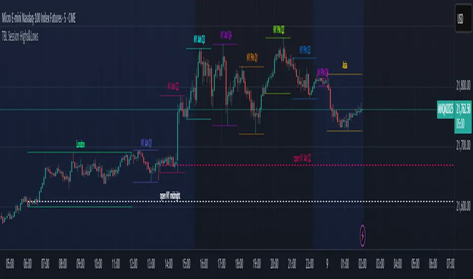
TBL Session Highs&LowsBL Session Highs&Lows is a versatile intraday tool that highlights key price levels within up to 11 configurable trading sessions. It displays session highs, lows, and optional open levels, with customizable lines, labels, and boxes — perfect for tracking price behavior across sessions like Asia, London, and New York.
🔧 Key Features
🧩 Up to 11 fully customizable sessions
📍 High, Low, and Open lines with adjustable color, style, and width
🧱 Optional boxes showing session range, dynamically colored based on price movement
🏷️ Session labels for visual orientation
🔁 Extendable lines to project levels beyond the session
🌐 Custom time zone support for each session
🎨 Fully customizable visuals for clear chart integration
📈 Designed for:
Intraday session tracking (e.g., Asia, London, NY)
Session-based strategies (breakouts, reversals, liquidity zones)
Open-level reference (e.g., NY open)
Visual separation of trading periods
Example Scenarios:
🟦 "Asia" session: 18:00–00:00 GMT-4 with full box and lines
🟩 "London" session: 00:00–06:00 with high/low lines only
🟥 Segmented NY sessions (Q1–Q4) for fine-grained intraday tracking
✅ Tip: Enable only the sessions you need to keep your chart clean and focused.
Cari dalam skrip untuk "11月1日是什么星座"
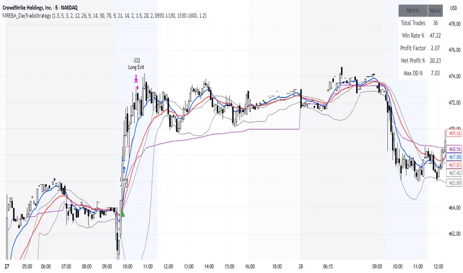
MACD + RSI + EMA + BB + ATR Day Trading StrategyEntry Conditions and Signals
The strategy implements a multi-layered filtering approach to entry conditions, requiring alignment across technical indicators, timeframes, and market conditions .
Long Entry Requirements
Trend Filter: Fast EMA (9) must be above Slow EMA (21), price must be above Fast EMA, and higher timeframe must confirm uptrend
MACD Signal: MACD line crosses above signal line, indicating increasing bullish momentum
RSI Condition: RSI below 70 (not overbought) but above 40 (showing momentum)
Volume & Volatility: Current volume exceeds 1.2x 20-period average and ATR shows sufficient market movement
Time Filter: Trading occurs during optimal hours (9:30-11:30 AM ET) when market volatility is typically highest
Exit Strategies
The strategy employs multiple exit mechanisms to adapt to changing market conditions and protect profits :
Stop Loss Management
Initial Stop: Placed at 2.0x ATR from entry price, adapting to current market volatility
Trailing Stop: 1.5x ATR trailing stop that moves up (for longs) or down (for shorts) as price moves favorably
Time-Based Exits: All positions closed by end of trading day (4:00 PM ET) to avoid overnight risk
Best Practices for Implementation
Settings
Chart Setup: 5-minute timeframe for execution with 15-minute chart for trend confirmation
Session Times: Focus on 9:30-11:30 AM ET trading for highest volatility and opportunity
Bear Market Probability Model# Bear Market Probability Model: A Multi-Factor Risk Assessment Framework
The Bear Market Probability Model represents a comprehensive quantitative framework for assessing systemic market risk through the integration of 13 distinct risk factors across four analytical categories: macroeconomic indicators, technical analysis factors, market sentiment measures, and market breadth metrics. This indicator synthesizes established financial research methodologies to provide real-time probabilistic assessments of impending bear market conditions, offering institutional-grade risk management capabilities to retail and professional traders alike.
## Theoretical Foundation
### Historical Context of Bear Market Prediction
Bear market prediction has been a central focus of financial research since the seminal work of Dow (1901) and the subsequent development of technical analysis theory. The challenge of predicting market downturns gained renewed academic attention following the market crashes of 1929, 1987, 2000, and 2008, leading to the development of sophisticated multi-factor models.
Fama and French (1989) demonstrated that certain financial variables possess predictive power for stock returns, particularly during market stress periods. Their three-factor model laid the groundwork for multi-dimensional risk assessment, which this indicator extends through the incorporation of real-time market microstructure data.
### Methodological Framework
The model employs a weighted composite scoring methodology based on the theoretical framework established by Campbell and Shiller (1998) for market valuation assessment, extended through the incorporation of high-frequency sentiment and technical indicators as proposed by Baker and Wurgler (2006) in their seminal work on investor sentiment.
The mathematical foundation follows the general form:
Bear Market Probability = Σ(Wi × Ci) / ΣWi × 100
Where:
- Wi = Category weight (i = 1,2,3,4)
- Ci = Normalized category score
- Categories: Macroeconomic, Technical, Sentiment, Breadth
## Component Analysis
### 1. Macroeconomic Risk Factors
#### Yield Curve Analysis
The inclusion of yield curve inversion as a primary predictor follows extensive research by Estrella and Mishkin (1998), who demonstrated that the term spread between 3-month and 10-year Treasury securities has historically preceded all major recessions since 1969. The model incorporates both the 2Y-10Y and 3M-10Y spreads to capture different aspects of monetary policy expectations.
Implementation:
- 2Y-10Y Spread: Captures market expectations of monetary policy trajectory
- 3M-10Y Spread: Traditional recession predictor with 12-18 month lead time
Scientific Basis: Harvey (1988) and subsequent research by Ang, Piazzesi, and Wei (2006) established the theoretical foundation linking yield curve inversions to economic contractions through the expectations hypothesis of the term structure.
#### Credit Risk Premium Assessment
High-yield credit spreads serve as a real-time gauge of systemic risk, following the methodology established by Gilchrist and Zakrajšek (2012) in their excess bond premium research. The model incorporates the ICE BofA High Yield Master II Option-Adjusted Spread as a proxy for credit market stress.
Threshold Calibration:
- Normal conditions: < 350 basis points
- Elevated risk: 350-500 basis points
- Severe stress: > 500 basis points
#### Currency and Commodity Stress Indicators
The US Dollar Index (DXY) momentum serves as a risk-off indicator, while the Gold-to-Oil ratio captures commodity market stress dynamics. This approach follows the methodology of Akram (2009) and Beckmann, Berger, and Czudaj (2015) in analyzing commodity-currency relationships during market stress.
### 2. Technical Analysis Factors
#### Multi-Timeframe Moving Average Analysis
The technical component incorporates the well-established moving average convergence methodology, drawing from the work of Brock, Lakonishok, and LeBaron (1992), who provided empirical evidence for the profitability of technical trading rules.
Implementation:
- Price relative to 50-day and 200-day simple moving averages
- Moving average convergence/divergence analysis
- Multi-timeframe MACD assessment (daily and weekly)
#### Momentum and Volatility Analysis
The model integrates Relative Strength Index (RSI) analysis following Wilder's (1978) original methodology, combined with maximum drawdown analysis based on the work of Magdon-Ismail and Atiya (2004) on optimal drawdown measurement.
### 3. Market Sentiment Factors
#### Volatility Index Analysis
The VIX component follows the established research of Whaley (2009) and subsequent work by Bekaert and Hoerova (2014) on VIX as a predictor of market stress. The model incorporates both absolute VIX levels and relative VIX spikes compared to the 20-day moving average.
Calibration:
- Low volatility: VIX < 20
- Elevated concern: VIX 20-25
- High fear: VIX > 25
- Panic conditions: VIX > 30
#### Put-Call Ratio Analysis
Options flow analysis through put-call ratios provides insight into sophisticated investor positioning, following the methodology established by Pan and Poteshman (2006) in their analysis of informed trading in options markets.
### 4. Market Breadth Factors
#### Advance-Decline Analysis
Market breadth assessment follows the classic work of Fosback (1976) and subsequent research by Brown and Cliff (2004) on market breadth as a predictor of future returns.
Components:
- Daily advance-decline ratio
- Advance-decline line momentum
- McClellan Oscillator (Ema19 - Ema39 of A-D difference)
#### New Highs-New Lows Analysis
The new highs-new lows ratio serves as a market leadership indicator, based on the research of Zweig (1986) and validated in academic literature by Zarowin (1990).
## Dynamic Threshold Methodology
The model incorporates adaptive thresholds based on rolling volatility and trend analysis, following the methodology established by Pagan and Sossounov (2003) for business cycle dating. This approach allows the model to adjust sensitivity based on prevailing market conditions.
Dynamic Threshold Calculation:
- Warning Level: Base threshold ± (Volatility × 1.0)
- Danger Level: Base threshold ± (Volatility × 1.5)
- Bounds: ±10-20 points from base threshold
## Professional Implementation
### Institutional Usage Patterns
Professional risk managers typically employ multi-factor bear market models in several contexts:
#### 1. Portfolio Risk Management
- Tactical Asset Allocation: Reducing equity exposure when probability exceeds 60-70%
- Hedging Strategies: Implementing protective puts or VIX calls when warning thresholds are breached
- Sector Rotation: Shifting from growth to defensive sectors during elevated risk periods
#### 2. Risk Budgeting
- Value-at-Risk Adjustment: Incorporating bear market probability into VaR calculations
- Stress Testing: Using probability levels to calibrate stress test scenarios
- Capital Requirements: Adjusting regulatory capital based on systemic risk assessment
#### 3. Client Communication
- Risk Reporting: Quantifying market risk for client presentations
- Investment Committee Decisions: Providing objective risk metrics for strategic decisions
- Performance Attribution: Explaining defensive positioning during market stress
### Implementation Framework
Professional traders typically implement such models through:
#### Signal Hierarchy:
1. Probability < 30%: Normal risk positioning
2. Probability 30-50%: Increased hedging, reduced leverage
3. Probability 50-70%: Defensive positioning, cash building
4. Probability > 70%: Maximum defensive posture, short exposure consideration
#### Risk Management Integration:
- Position Sizing: Inverse relationship between probability and position size
- Stop-Loss Adjustment: Tighter stops during elevated risk periods
- Correlation Monitoring: Increased attention to cross-asset correlations
## Strengths and Advantages
### 1. Comprehensive Coverage
The model's primary strength lies in its multi-dimensional approach, avoiding the single-factor bias that has historically plagued market timing models. By incorporating macroeconomic, technical, sentiment, and breadth factors, the model provides robust risk assessment across different market regimes.
### 2. Dynamic Adaptability
The adaptive threshold mechanism allows the model to adjust sensitivity based on prevailing volatility conditions, reducing false signals during low-volatility periods and maintaining sensitivity during high-volatility regimes.
### 3. Real-Time Processing
Unlike traditional academic models that rely on monthly or quarterly data, this indicator processes daily market data, providing timely risk assessment for active portfolio management.
### 4. Transparency and Interpretability
The component-based structure allows users to understand which factors are driving risk assessment, enabling informed decision-making about model signals.
### 5. Historical Validation
Each component has been validated in academic literature, providing theoretical foundation for the model's predictive power.
## Limitations and Weaknesses
### 1. Data Dependencies
The model's effectiveness depends heavily on the availability and quality of real-time economic data. Federal Reserve Economic Data (FRED) updates may have lags that could impact model responsiveness during rapidly evolving market conditions.
### 2. Regime Change Sensitivity
Like most quantitative models, the indicator may struggle during unprecedented market conditions or structural regime changes where historical relationships break down (Taleb, 2007).
### 3. False Signal Risk
Multi-factor models inherently face the challenge of balancing sensitivity with specificity. The model may generate false positive signals during normal market volatility periods.
### 4. Currency and Geographic Bias
The model focuses primarily on US market indicators, potentially limiting its effectiveness for global portfolio management or non-USD denominated assets.
### 5. Correlation Breakdown
During extreme market stress, correlations between risk factors may increase dramatically, reducing the model's diversification benefits (Forbes and Rigobon, 2002).
## References
Akram, Q. F. (2009). Commodity prices, interest rates and the dollar. Energy Economics, 31(6), 838-851.
Ang, A., Piazzesi, M., & Wei, M. (2006). What does the yield curve tell us about GDP growth? Journal of Econometrics, 131(1-2), 359-403.
Baker, M., & Wurgler, J. (2006). Investor sentiment and the cross‐section of stock returns. The Journal of Finance, 61(4), 1645-1680.
Baker, S. R., Bloom, N., & Davis, S. J. (2016). Measuring economic policy uncertainty. The Quarterly Journal of Economics, 131(4), 1593-1636.
Barber, B. M., & Odean, T. (2001). Boys will be boys: Gender, overconfidence, and common stock investment. The Quarterly Journal of Economics, 116(1), 261-292.
Beckmann, J., Berger, T., & Czudaj, R. (2015). Does gold act as a hedge or a safe haven for stocks? A smooth transition approach. Economic Modelling, 48, 16-24.
Bekaert, G., & Hoerova, M. (2014). The VIX, the variance premium and stock market volatility. Journal of Econometrics, 183(2), 181-192.
Brock, W., Lakonishok, J., & LeBaron, B. (1992). Simple technical trading rules and the stochastic properties of stock returns. The Journal of Finance, 47(5), 1731-1764.
Brown, G. W., & Cliff, M. T. (2004). Investor sentiment and the near-term stock market. Journal of Empirical Finance, 11(1), 1-27.
Campbell, J. Y., & Shiller, R. J. (1998). Valuation ratios and the long-run stock market outlook. The Journal of Portfolio Management, 24(2), 11-26.
Dow, C. H. (1901). Scientific stock speculation. The Magazine of Wall Street.
Estrella, A., & Mishkin, F. S. (1998). Predicting US recessions: Financial variables as leading indicators. Review of Economics and Statistics, 80(1), 45-61.
Fama, E. F., & French, K. R. (1989). Business conditions and expected returns on stocks and bonds. Journal of Financial Economics, 25(1), 23-49.
Forbes, K. J., & Rigobon, R. (2002). No contagion, only interdependence: measuring stock market comovements. The Journal of Finance, 57(5), 2223-2261.
Fosback, N. G. (1976). Stock market logic: A sophisticated approach to profits on Wall Street. The Institute for Econometric Research.
Gilchrist, S., & Zakrajšek, E. (2012). Credit spreads and business cycle fluctuations. American Economic Review, 102(4), 1692-1720.
Harvey, C. R. (1988). The real term structure and consumption growth. Journal of Financial Economics, 22(2), 305-333.
Kahneman, D., & Tversky, A. (1979). Prospect theory: An analysis of decision under risk. Econometrica, 47(2), 263-291.
Magdon-Ismail, M., & Atiya, A. F. (2004). Maximum drawdown. Risk, 17(10), 99-102.
Nickerson, R. S. (1998). Confirmation bias: A ubiquitous phenomenon in many guises. Review of General Psychology, 2(2), 175-220.
Pagan, A. R., & Sossounov, K. A. (2003). A simple framework for analysing bull and bear markets. Journal of Applied Econometrics, 18(1), 23-46.
Pan, J., & Poteshman, A. M. (2006). The information in option volume for future stock prices. The Review of Financial Studies, 19(3), 871-908.
Taleb, N. N. (2007). The black swan: The impact of the highly improbable. Random House.
Whaley, R. E. (2009). Understanding the VIX. The Journal of Portfolio Management, 35(3), 98-105.
Wilder, J. W. (1978). New concepts in technical trading systems. Trend Research.
Zarowin, P. (1990). Size, seasonality, and stock market overreaction. Journal of Financial and Quantitative Analysis, 25(1), 113-125.
Zweig, M. E. (1986). Winning on Wall Street. Warner Books.

LANZ Strategy 2.0 [Backtest]🔷 LANZ Strategy 2.0 — Structural Breakout Logic with Dynamic Swing Protection
LANZ Strategy 2.0 is a precision-focused backtesting system built for intraday traders who rely on structural confirmations before the London session to guide directional bias. This tool uses smart swing detection, risk-defined position sizing, and strict time-based execution to simulate real trading conditions with clarity and control.
🧠 Core Components:
Structural Confirmation (Trend & BoS): Detects trend direction and break of structure (BoS) using a three-swing logic, aligning trade entries with valid structural movement.
Time-Based Execution: Trades are triggered exclusively at 02:00 a.m. New York time, ensuring disciplined and repeatable intraday testing.
Swing-Based SL Models: Traders can select between three stop-loss protection types:
First Swing: Most recent structural level
Second Swing: Prior level
Full Coverage: All recent swing levels + configurable pip buffer
Dynamic TP Calculation: Take-Profit is projected as a risk-based multiple (RR), fully adjustable via input.
Capital-Based Risk Management: Risk is defined as a percentage of a fixed account size (e.g., $100 per trade from $10,000), and lot size is automatically calculated based on SL distance.
Fallback Entry Logic: If structural breakout is present but trend is not confirmed, a secondary entry is triggered.
End-of-Session Management: Any open trades are automatically closed at 11:45 a.m. NY time, with optional manual labeling or review.
📊 Visual Features (Optional in Indicator Version):
(Note: Visuals apply to the indicator version of LANZ 2.0, not this backtest script)
Swing level labels (1st, 2nd) and dynamic SL/TP lines.
Real-time session coloring for clarity: Pre-London, Entry Window, and NY Close.
Outcome labels: +RR, -RR, or net % at close.
Auto-cleanup of previous drawings for a clean chart per session.
⚙️ How It Works:
Detects last trend and BoS using swing logic before 02:00 a.m. NY.
At 02:00 a.m., evaluates directional bias and executes BUY or SELL if confirmed.
Applies selected SL logic (1st, 2nd, or full swing protection).
Sets TP based on the RR multiplier.
Closes the trade either on SL, TP, or at 11:45 a.m. NY manually.
🔔 Alerts:
Time-of-day alert at 02:00 a.m. NY to monitor execution.
Can be extended to cover SL/TP triggers or new BoS events.
📝 Notes:
Designed for backtesting precision and discretionary decision-making.
Ideal for Forex pairs, indices, or assets active during the London session.
Fully customizable: session timing, swing logic, SL buffer, and RR.
👤 Credits:
Strategy built by @rau_u_lanz using Pine Script v6, combining structural logic, capital-based risk control, and London-session timing in a backtest-ready framework for traders who demand accuracy and structure.

Why EMA Isn't What You Think It IsMany new traders adopt the Exponential Moving Average (EMA) believing it's simply a "better Simple Moving Average (SMA)". This common misconception leads to fundamental misunderstandings about how EMA works and when to use it.
EMA and SMA differ at their core. SMA use a window of finite number of data points, giving equal weight to each data point in the calculation period. This makes SMA a Finite Impulse Response (FIR) filter in signal processing terms. Remember that FIR means that "all that we need is the 'period' number of data points" to calculate the filter value. Anything beyond the given period is not relevant to FIR filters – much like how a security camera with 14-day storage automatically overwrites older footage, making last month's activity completely invisible regardless of how important it might have been.
EMA, however, is an Infinite Impulse Response (IIR) filter. It uses ALL historical data, with each past price having a diminishing - but never zero - influence on the calculated value. This creates an EMA response that extends infinitely into the past—not just for the last N periods. IIR filters cannot be precise if we give them only a 'period' number of data to work on - they will be off-target significantly due to lack of context, like trying to understand Game of Thrones by watching only the final season and wondering why everyone's so upset about that dragon lady going full pyromaniac.
If we only consider a number of data points equal to the EMA's period, we are capturing no more than 86.5% of the total weight of the EMA calculation. Relying on he period window alone (the warm-up period) will provide only 1 - (1 / e^2) weights, which is approximately 1−0.1353 = 0.8647 = 86.5%. That's like claiming you've read a book when you've skipped the first few chapters – technically, you got most of it, but you probably miss some crucial early context.
▶️ What is period in EMA used for?
What does a period parameter really mean for EMA? When we select a 15-period EMA, we're not selecting a window of 15 data points as with an SMA. Instead, we are using that number to calculate a decay factor (α) that determines how quickly older data loses influence in EMA result. Every trader knows EMA calculation: α = 1 / (1+period) – or at least every trader claims to know this while secretly checking the formula when they need it.
Thinking in terms of "period" seriously restricts EMA. The α parameter can be - should be! - any value between 0.0 and 1.0, offering infinite tuning possibilities of the indicator. When we limit ourselves to whole-number periods that we use in FIR indicators, we can only access a small subset of possible IIR calculations – it's like having access to the entire RGB color spectrum with 16.7 million possible colors but stubbornly sticking to the 8 basic crayons in a child's first art set because the coloring book only mentioned those by name.
For example:
Period 10 → alpha = 0.1818
Period 11 → alpha = 0.1667
What about wanting an alpha of 0.17, which might yield superior returns in your strategy that uses EMA? No whole-number period can provide this! Direct α parameterization offers more precision, much like how an analog tuner lets you find the perfect radio frequency while digital presets force you to choose only from predetermined stations, potentially missing the clearest signal sitting right between channels.
Sidenote: the choice of α = 1 / (1+period) is just a convention from 1970s, probably started by J. Welles Wilder, who popularized the use of the 14-day EMA. It was designed to create an approximate equivalence between EMA and SMA over the same number of periods, even thought SMA needs a period window (as it is FIR filter) and EMA doesn't. In reality, the decay factor α in EMA should be allowed any valye between 0.0 and 1.0, not just some discrete values derived from an integer-based period! Algorithmic systems should find the best α decay for EMA directly, allowing the system to fine-tune at will and not through conversion of integer period to float α decay – though this might put a few traditionalist traders into early retirement. Well, to prevent that, most traditionalist implementations of EMA only use period and no alpha at all. Heaven forbid we disturb people who print their charts on paper, draw trendlines with rulers, and insist the market "feels different" since computers do algotrading!
▶️ Calculating EMAs Efficiently
The standard textbook formula for EMA is:
EMA = CurrentPrice × alpha + PreviousEMA × (1 - alpha)
But did you know that a more efficient version exists, once you apply a tiny bit of high school algebra:
EMA = alpha × (CurrentPrice - PreviousEMA) + PreviousEMA
The first one requires three operations: 2 multiplications + 1 addition. The second one also requires three ops: 1 multiplication + 1 addition + 1 subtraction.
That's pathetic, you say? Not worth implementing? In most computational models, multiplications cost much more than additions/subtractions – much like how ordering dessert costs more than asking for a water refill at restaurants.
Relative CPU cost of float operations :
Addition/Subtraction: ~1 cycle
Multiplication: ~5 cycles (depending on precision and architecture)
Now you see the difference? 2 * 5 + 1 = 11 against 5 + 1 + 1 = 7. That is ≈ 36.36% efficiency gain just by swapping formulas around! And making your high school math teacher proud enough to finally put your test on the refrigerator.
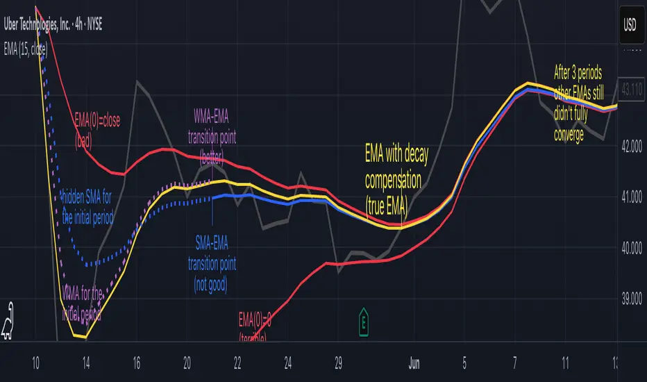
▶️ The Warmup Problem: how to start the EMA sequence right
How do we calculate the first EMA value when there's no previous EMA available? Let's see some possible options used throughout the history:
Start with zero : EMA(0) = 0. This creates stupidly large distortion until enough bars pass for the horrible effect to diminish – like starting a trading account with zero balance but backdating a year of missed trades, then watching your balance struggle to climb out of a phantom debt for months.
Start with first price : EMA(0) = first price. This is better than starting with zero, but still causes initial distortion that will be extra-bad if the first price is an outlier – like forming your entire opinion of a stock based solely on its IPO day price, then wondering why your model is tanking for weeks afterward.
Use SMA for warmup : This is the tradition from the pencil-and-paper era of technical analysis – when calculators were luxury items and "algorithmic trading" meant your broker had neat handwriting. We first calculate an SMA over the initial period, then kickstart the EMA with this average value. It's widely used due to tradition, not merit, creating a mathematical Frankenstein that uses an FIR filter (SMA) during the initial period before abruptly switching to an IIR filter (EMA). This methodology is so aesthetically offensive (abrupt kink on the transition from SMA to EMA) that charting platforms hide these early values entirely, pretending EMA simply doesn't exist until the warmup period passes – the technical analysis equivalent of sweeping dust under the rug.
Use WMA for warmup : This one was never popular because it is harder to calculate with a pencil - compared to using simple SMA for warmup. Weighted Moving Average provides a much better approximation of a starting value as its linear descending profile is much closer to the EMA's decay profile.
These methods all share one problem: they produce inaccurate initial values that traders often hide or discard, much like how hedge funds conveniently report awesome performance "since strategy inception" only after their disastrous first quarter has been surgically removed from the track record.
▶️ A Better Way to start EMA: Decaying compensation
Think of it this way: An ideal EMA uses an infinite history of prices, but we only have data starting from a specific point. This creates a problem - our EMA starts with an incorrect assumption that all previous prices were all zero, all close, or all average – like trying to write someone's biography but only having information about their life since last Tuesday.
But there is a better way. It requires more than high school math comprehension and is more computationally intensive, but is mathematically correct and numerically stable. This approach involves compensating calculated EMA values for the "phantom data" that would have existed before our first price point.
Here's how phantom data compensation works:
We start our normal EMA calculation:
EMA_today = EMA_yesterday + α × (Price_today - EMA_yesterday)
But we add a correction factor that adjusts for the missing history:
Correction = 1 at the start
Correction = Correction × (1-α) after each calculation
We then apply this correction:
True_EMA = Raw_EMA / (1-Correction)
This correction factor starts at 1 (full compensation effect) and gets exponentially smaller with each new price bar. After enough data points, the correction becomes so small (i.e., below 0.0000000001) that we can stop applying it as it is no longer relevant.
Let's see how this works in practice:
For the first price bar:
Raw_EMA = 0
Correction = 1
True_EMA = Price (since 0 ÷ (1-1) is undefined, we use the first price)
For the second price bar:
Raw_EMA = α × (Price_2 - 0) + 0 = α × Price_2
Correction = 1 × (1-α) = (1-α)
True_EMA = α × Price_2 ÷ (1-(1-α)) = Price_2
For the third price bar:
Raw_EMA updates using the standard formula
Correction = (1-α) × (1-α) = (1-α)²
True_EMA = Raw_EMA ÷ (1-(1-α)²)
With each new price, the correction factor shrinks exponentially. After about -log₁₀(1e-10)/log₁₀(1-α) bars, the correction becomes negligible, and our EMA calculation matches what we would get if we had infinite historical data.
This approach provides accurate EMA values from the very first calculation. There's no need to use SMA for warmup or discard early values before output converges - EMA is mathematically correct from first value, ready to party without the awkward warmup phase.
Here is Pine Script 6 implementation of EMA that can take alpha parameter directly (or period if desired), returns valid values from the start, is resilient to dirty input values, uses decaying compensator instead of SMA, and uses the least amount of computational cycles possible.
// Enhanced EMA function with proper initialization and efficient calculation
ema(series float source, simple int period=0, simple float alpha=0)=>
// Input validation - one of alpha or period must be provided
if alpha<=0 and period<=0
runtime.error("Alpha or period must be provided")
// Calculate alpha from period if alpha not directly specified
float a = alpha > 0 ? alpha : 2.0 / math.max(period, 1)
// Initialize variables for EMA calculation
var float ema = na // Stores raw EMA value
var float result = na // Stores final corrected EMA
var float e = 1.0 // Decay compensation factor
var bool warmup = true // Flag for warmup phase
if not na(source)
if na(ema)
// First value case - initialize EMA to zero
// (we'll correct this immediately with the compensation)
ema := 0
result := source
else
// Standard EMA calculation (optimized formula)
ema := a * (source - ema) + ema
if warmup
// During warmup phase, apply decay compensation
e *= (1-a) // Update decay factor
float c = 1.0 / (1.0 - e) // Calculate correction multiplier
result := c * ema // Apply correction
// Stop warmup phase when correction becomes negligible
if e <= 1e-10
warmup := false
else
// After warmup, EMA operates without correction
result := ema
result // Return the properly compensated EMA value
▶️ CONCLUSION
EMA isn't just a "better SMA"—it is a fundamentally different tool, like how a submarine differs from a sailboat – both float, but the similarities end there. EMA responds to inputs differently, weighs historical data differently, and requires different initialization techniques.
By understanding these differences, traders can make more informed decisions about when and how to use EMA in trading strategies. And as EMA is embedded in so many other complex and compound indicators and strategies, if system uses tainted and inferior EMA calculatiomn, it is doing a disservice to all derivative indicators too – like building a skyscraper on a foundation of Jell-O.
The next time you add an EMA to your chart, remember: you're not just looking at a "faster moving average." You're using an INFINITE IMPULSE RESPONSE filter that carries the echo of all previous price actions, properly weighted to help make better trading decisions.
EMA done right might significantly improve the quality of all signals, strategies, and trades that rely on EMA somewhere deep in its algorithmic bowels – proving once again that math skills are indeed useful after high school, no matter what your guidance counselor told you.
LANZ Strategy 2.0🔷 LANZ Strategy 2.0 — London Breakout Confirmation with Structural Swing Protection
LANZ Strategy 2.0 is a structured trading system that leverages the last confirmed market direction before the London session to define directional bias and manage trades based on key structural swing levels. It is tailored for intraday traders looking to capitalize on early London volatility with built-in risk management and visual clarity.
🧠 Core Components:
Directional Confirmation (Pre-London Bias): Validates the last breakout or structural move from the 15-minute timeframe before 02:15 a.m. New York time (start of the London session), establishing the expected market direction.
Time-Based Execution: Executes potential entries strictly at 02:15 a.m. NY time, using market structure to support Long or Short bias.
Dynamic Swing-Based SL System: Allows user to select between three SL protection models: First Swing (most recent structural point) Second Swing (prior level) Total Coverage (includes both swings + extra buffer) This supports flexibility based on trader profile or market conditions.
Visual Risk Mapping: All SL and TP levels are clearly plotted.
End-of-Session Management: Positions are automatically evaluated for closure at 11:45 a.m. NY time. SL, TP, or manual close outcomes are labeled accordingly.
📊 Visual Features:
Labels for 1st and 2nd swing levels upon entry.
Dynamic lines projecting SL/TP levels toward the end of the session.
Session background coloring for Pre-London, Execution, and NY sessions.
Real-time percentage outcome labels (+2.00%, -1.00%, or net % at session end).
Automatic deletion of previous visuals on new entries for clean charting.
⚙️ How It Works:
Detects last structural breakout on the 15m timeframe before 02:15 a.m. NY.
On the 02:15 a.m. candle, executes a Long or Short logic entry.
Plots corresponding SL and TP based on selected swing model.
Monitors price action: If TP or SL is hit, labels it accordingly. If no exit is hit, trade closes manually at 11:45 a.m. NY with net result shown.
Optional logic to reverse entries if market structure breaks before execution.
🔔 Alerts:
Daily execution alert at 02:15 a.m. NY (prompting manual review or action).
Optional alert logic can be extended for SL/TP hits or structure breaks.
📝 Notes:
Designed for semi-automated or discretionary intraday trading.
Best used on Forex pairs or indices with strong London session behavior.
Adjustable parameters include session hours, swing SL type, and buffer settings.
Credits:
Developed by LANZ, this script combines time-based execution with dynamic structure protection, offering a disciplined framework for participating in the London session breakout with clear visuals and risk logic.

Time-Based Fair Value Gaps (FVG) with Inversions (iFVG)Overview
The Time-Based Fair Value Gaps (FVG) with Inversions (iFVG) (ICT/SMT) indicator is a specialized tool designed for traders using Inner Circle Trader (ICT) methodologies. Inspired by LuxAlgo's Fair Value Gap indicator, this script introduces significant enhancements by integrating ICT principles, focusing on precise time-based FVG detection, inversion tracking, and retest signals tailored for institutional trading strategies. Unlike LuxAlgo’s general FVG approach, this indicator filters FVGs within customizable 10-minute windows aligned with ICT’s macro timeframes and incorporates ICT-specific concepts like mitigation, liquidity grabs, and session-based gap prioritization.
This tool is optimized for 1–5 minute charts, though probably best for 1 minute charts, identifying bullish and bearish FVGs, tracking their mitigation into inverted FVGs (iFVGs) as key support/resistance zones, and generating retest signals with customizable “Close” or “Wick” confirmation. Features like ATR-based filtering, optional FVG labels, mitigation removal, and session-specific FVG detection (e.g., first FVG in AM/PM sessions) make it a powerful tool for ICT traders.
Originality and Improvements
While inspired by LuxAlgo’s FVG indicator (credit to LuxAlgo for their foundational work), this script significantly extends the original concept by:
1. Time-Based FVG Detection: Unlike LuxAlgo’s continuous FVG identification, this script filters FVGs within user-defined 10-minute windows each hour (:00–:10, :10–:20, etc.), aligning with ICT’s emphasis on specific periods of institutional activity, such as hourly opens/closes or kill zones (e.g., New York 7:00–11:00 AM EST). This ensures FVGs are relevant to high-probability ICT setups.
2. Session-Specific First FVG Option: A unique feature allows traders to display only the first FVG in ICT-defined AM (9:30–10:00 AM EST) or PM (1:30–2:00 PM EST) sessions, reflecting ICT’s focus on initial market imbalances during key liquidity events.
3. ICT-Driven Mitigation and Inversion Logic: The script tracks FVG mitigation (when price closes through a gap) and converts mitigated FVGs into iFVGs, which serve as ICT-style support/resistance zones. This aligns with ICT’s view that mitigated gaps become critical reversal points, unlike LuxAlgo’s simpler gap display.
4. Customizable Retest Signals: Retest signals for iFVGs are configurable for “Close” (conservative, requiring candle body confirmation) or “Wick” (faster, using highs/lows), catering to ICT traders’ need for precise entry timing during liquidity grabs or Judas swings.
5. ATR Filtering and Mitigation Removal: An optional ATR filter ensures only significant FVGs are displayed, reducing noise, while mitigation removal declutters the chart by removing filled gaps, aligning with ICT’s principle that mitigated gaps lose relevance unless inverted.
6. Timezone and Timeframe Safeguards: A timezone offset setting aligns FVG detection with EST for ICT’s New York-centric strategies, and a timeframe warning alerts users to avoid ≥1-hour charts, ensuring accuracy in time-based filtering.
These enhancements make the script a distinct tool that builds on LuxAlgo’s foundation while offering ICT traders a tailored, high-precision solution.
How It Works
FVG Detection
FVGs are identified when a candle’s low is higher than the high of two candles prior (bullish FVG) or a candle’s high is lower than the low of two candles prior (bearish FVG). Detection is restricted to:
• User-selected 10-minute windows (e.g., :00–:10, :50–:60) to capture ICT-relevant periods like hourly transitions.
• AM/PM session first FVGs (if enabled), focusing on 9:30–10:00 AM or 1:30–2:00 PM EST for key market opens.
An optional ATR filter (default: 0.25× ATR) ensures only gaps larger than the threshold are displayed, prioritizing significant imbalances.
Mitigation and Inversion
When price closes through an FVG (e.g., below a bullish FVG’s bottom), the FVG is mitigated and becomes an iFVG, plotted as a support/resistance zone. iFVGs are critical in ICT for identifying reversal points where institutional orders accumulate.
Retest Signals
The script generates signals when price retests an iFVG:
• Close: Triggers when the candle body confirms the retest (conservative, lower noise).
• Wick: Triggers when the candle’s high/low touches the iFVG (faster, higher sensitivity). Signals are visualized with triangular markers (▲ for bullish, ▼ for bearish) and can trigger alerts.
Visualization
• FVGs: Displayed as colored boxes (green for bullish, red for bearish) with optional “Bull FVG”/“Bear FVG” labels.
• iFVGs: Shown as extended boxes with dashed midlines, limited to the user-defined number of recent zones (default: 5).
• Mitigation Removal: Mitigated FVGs/iFVGs are removed (if enabled) to keep the chart clean.
How to Use
Recommended Settings
• Timeframe: Use 1–5 minute charts for precision, avoiding ≥1-hour timeframes (a warning label appears if misconfigured).
• Time Windows: Enable :00–:10 and :50–:60 for hourly open/close FVGs, or use the “Show only 1st presented FVG” option for AM/PM session focus.
• ATR Filter: Keep enabled (multiplier 0.25–0.5) for significant gaps; disable on 1-minute charts for more FVGs during volatility.
• Signal Preference: Use “Close” for conservative entries, “Wick” for aggressive setups.
• Timezone Offset: Set to -5 for EST (or -4 for EDT) to align with ICT’s New York session.
Trading Strategy
1. Macro Timeframes: Focus on New York (7:00–11:00 AM EST) or London (2:00–5:00 AM EST) kill zones for high institutional activity.
2. FVG Entries: Trade bullish FVGs as support in uptrends or bearish FVGs as resistance in downtrends, especially in :00–:10 or :50–:60 windows.
3. iFVG Retests: Enter on retest signals (▲/▼) during liquidity grabs or Judas swings, using “Close” for confirmation or “Wick” for speed.
4. Session FVGs: Use the “Show only 1st presented FVG” option to target the first gap in AM/PM sessions, often tied to ICT’s market maker algorithms.
5. Risk Management: Combine with ICT concepts like order blocks or breaker blocks for confluence, and set stops beyond FVG/iFVG boundaries.
Alerts
Set alerts for:
• “Bullish FVG Detected”/“Bearish FVG Detected”: New FVGs in selected windows.
• “Bullish Signal”/“Bearish Signal”: iFVG retest confirmations.
Settings Description
• Show Last (1–100, default: 5): Number of recent iFVGs to display. Lower values reduce clutter.
• Show only 1st presented FVG : Limits FVGs to the first in 9:30–10:00 AM or 1:30–2:00 PM EST sessions (overrides time window checkboxes).
• Time Window Checkboxes: Enable/disable FVG detection in 10-minute windows (:00–:10, :10–:20, etc.). All enabled by default.
• Signal Preference: “Close” (default) or “Wick” for iFVG retest signals.
• Use ATR Filter: Enables ATR-based size filtering (default: true).
• ATR Multiplier (0–∞, default: 0.25): Sets FVG size threshold (higher values = larger gaps).
• Remove Mitigated FVGs: Removes filled FVGs/iFVGs (default: true).
• Show FVG Labels: Displays “Bull FVG”/“Bear FVG” labels (default: true).
• Timezone Offset (-12 to 12, default: -5): Aligns time windows with EST.
• Colors: Customize bullish (green), bearish (red), and midline (gray) colors.
Why Use This Indicator?
This indicator empowers ICT traders with a tool that goes beyond generic FVG detection, offering precise, time-filtered gaps and inversion tracking aligned with institutional trading principles. By focusing on ICT’s macro timeframes, session-specific imbalances, and customizable signal logic, it provides a clear edge for scalping, swing trading, or reversal setups in high-liquidity markets.
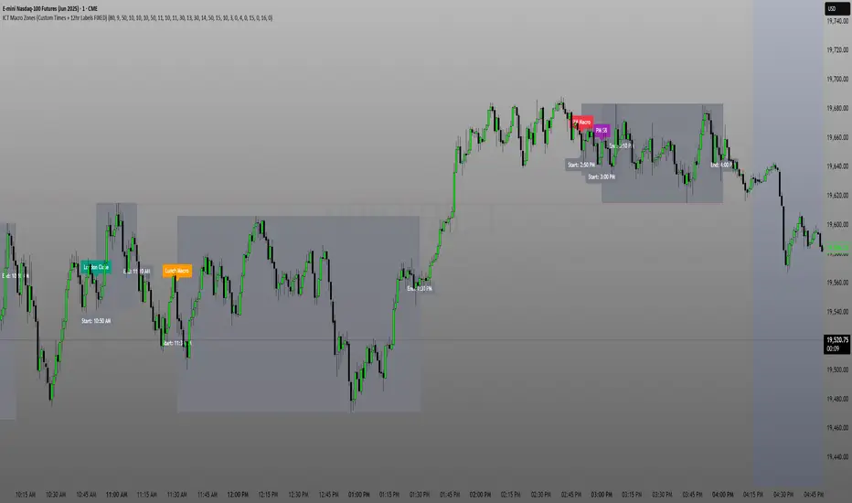
ICT Macro Zone Boxes w/ Individual H/L Tracking v3.1ICT Macro Zones (Grey Box Version
This indicator dynamically highlights key intraday time-based macro sessions using a clean, minimalistic grey box overlay, helping traders align with institutional trading cycles. Inspired by ICT (Inner Circle Trader) concepts, it tracks real-time highs and lows for each session and optionally extends the zone box after the session ends — making it a precision tool for intraday setups, order flow analysis, and macro-level liquidity sweeps.
### 🔍 **What It Does**
- Plots **six predefined macro sessions** used in Smart Money Concepts:
- AM Macro (09:50–10:10)
- London Close (10:50–11:10)
- Lunch Macro (11:30–13:30)
- PM Macro (14:50–15:10)
- London SB (03:00–04:00)
- PM SB (15:00–16:00)
- Each zone:
- **Tracks high and low dynamically** throughout the session.
- **Draws a consistent grey shaded box** to visualize price boundaries.
- **Displays a label** at the first bar of the session (optional).
- **Optionally extends** the box to the right after the session closes.
### 🧠 **How It Works**
- Uses Pine Script arrays to define each session’s time window, label, and color.
- Detects session entry using `time()` within a New York timezone context.
- High/Low values are updated per bar inside the session window.
- Once a session ends, the box is optionally closed and fixed in place.
- All visual zones use a standardized grey tone for clarity and consistency across charts.
### 🛠️ **Settings**
- **Shade Zone High→Low:** Enable/disable the grey macro box.
- **Extend Box After Session:** Keep the zone visible after it ends.
- **Show Entry Label:** Display a label at the start of each session.
### 🎯 **Why This Script is Unique**
Unlike basic session markers or colored backgrounds, this tool:
- Focuses on **macro moments of liquidity and reversal**, not just open/close times.
- Uses **per-session logic** to individually track price behavior inside key time windows.
- Supports **real-time high/low tracking and clean zone drawing**, ideal for Smart Money and ICT-style strategies.
Perfect — based on your list, here's a **bundle-style description** that not only explains the function of each script but also shows how they **work together** in a Smart Money/ICT workflow. This kind of cross-script explanation is exactly what TradingView wants to see to justify closed-source mashups or interdependent tools.
---
📚 ICT SMC Toolkit — Script Integration Guide
This set of advanced Smart Money Concept (SMC) tools is designed for traders who follow ICT-based methodologies, combining liquidity theory, time-based precision, and engineered confluences for high-probability trades. Each indicator is optimized to work both independently and synergistically, forming a comprehensive trading framework.
---
First FVG Custom Time Range
**Purpose:**
Plots the **first Fair Value Gap (FVG)** that appears within a defined session (e.g., NY Kill Zone, Custom range). Includes optional retest alerts.
**Best Used With:**
- Use with **ICT Macro Zones (Grey Box Version)** to isolate FVGs during high-probability times like AM Macro or PM SB.
- Combine with **Liquidity Levels** to assess whether FVGs form near swing points or liquidity voids.
---
ICT SMC Liquidity Grabs and OB s
**Purpose:**
Detects **liquidity grabs** (stop hunts above/below swing highs/lows) and **bullish/bearish order blocks**. Includes optional Fibonacci OTE levels for sniper entries.
**Best Used With:**
- Use with **ICT Turtle Soup (Reversal)** for confirmation after a liquidity grab.
- Combine with **Macro Zones** to catch order blocks forming inside timed macro windows.
- Match with **Smart Swing Levels** to confirm structure breaks before entry.
ICT SMC Liquidity Levels (Smart Swing Lows)
**Purpose:**
Automatically marks swing highs/lows based on user-defined lookbacks. Tracks whether those levels have been breached or respected.
**Best Used With:**
- Combine with **Turtle Soup** to detect if a swing level was swept, then reversed.
- Use with **Liquidity Grabs** to confirm a grab occurred at a meaningful structural point.
- Align with **Macro Zones** to understand when liquidity events occur within macro session timing.
ICT Turtle Soup (Liquidity Reversal)
**Purpose:**
Implements the classic ICT Turtle Soup model. Looks for swing failure and quick reversals after a liquidity sweep — ideal for catching traps.
Best Used With:
- Confirm with **Liquidity Grabs + OBs** to identify institutional activity at the reversal point.
- Use **Liquidity Levels** to ensure the reversal is happening at valid previous swing highs/lows.
- Amplify probability when pattern appears during **Macro Zones** or near the **First FVG**.
ICT Turtle Soup Ultimate V2
**Purpose:**
An enhanced, multi-layer version of the Turtle Soup setup that includes built-in liquidity checks, OTE levels, structure validation, and customizable visual output.
**Best Used With:**
- Use as an **entry signal generator** when other indicators (e.g., OBs, liquidity grabs) are aligned.
- Pair with **Macro Zones** for high-precision timing.
- Combine with **First FVG** to anticipate price rebalancing before explosive moves.
---
## 🧠 Workflow Example:
1. **Start with Macro Zones** to focus only on institutional trading windows.
2. Look for **Liquidity Grabs or Swing Sweeps** around key highs/lows.
3. Check for a **Turtle Soup Reversal** or **Order Block Reaction** near that level.
4. Confirm confluence with a **Fair Value Gap**.
5. Execute using the **OTE level** from the Liquidity Grabs + OB script.
---
Let me know which script you want to publish first — I’ll tailor its **individual TradingView description** and flag its ideal **“Best Used With” partners** to help users see the value in your ecosystem.
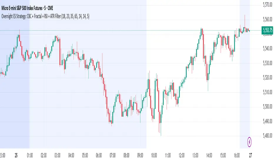
Overnight ES Strategy: CBC + Fractal + RSI + ATR FilterThis script is designed for overnight trading of the E-mini S&P 500 futures (ES) between 6 PM and 11 PM EST.
It combines multiple technical confluences to generate high-probability buy and sell signals, focusing on volatility-rich, low-liquidity evening sessions.
Key Features:
Candle Body Confluence (CBC) Approximation:
Identifies candles with small real bodies compared to total range, simulating consolidation zones where price is likely to reverse.
Williams Fractal Confirmation:
Detects local tops and bottoms based on 5-bar fractal reversal patterns, helping validate breakout or reversal points.
RSI Filter:
Ensures momentum is supportive — buys only when RSI < 35 (oversold) and sells only when RSI > 65 (overbought).
ATR Volatility Filter:
Trades are only allowed if the Average True Range (ATR) exceeds a user-defined threshold, filtering out low-volatility, risky environments.
Time Session Control:
Signals are only generated during the user-defined evening session (default: 6 PM to 11 PM EST) to match market behavior.
Real-Time Alerts Enabled:
Alerts can be set for BUY or SELL conditions, enabling mobile notifications, emails, or pop-ups without constant chart monitoring.
Recommended Settings:
Chart Timeframe: 15-minute or 30-minute candles
Assets: ES Mini (ES1!), NQ Mini, or other CME futures
Session: New York Time (EST)
ATR Threshold: Adjust based on market conditions; 5.0 suggested starting point for ES Mini on 15m.
Important:
This script only plots signals, it does not auto-execute trades.
Always backtest and paper trade before using live capital.
Volatility can vary; consider adjusting RSI and ATR filters based on market environment.
Credits:
Script designed based on confluence of price action, momentum, reversal structure, and volatility filtering principles used by professional traders.
Inspired by Candle Body Confluence (CBC) theory and Williams fractal techniques.
Umesh BC IST 3:30 AM Session Tracker + 4H Candles📌 IST 3:30 AM Session Tracker + 4H Candle Marker
This indicator is designed for traders who follow Indian Standard Time (IST) and want precise session tracking and 4H candle insights.
🔧 Features:
🕒 Daily Session Start at 3:30 AM IST
Automatically detects and marks the beginning of each new trading day based on 3:30 AM IST, not midnight.
Displays session Open, High, and Low lines.
Background shading for each session.
Customizable alert when a new day starts.
🟧 4H Candle Start Markers (IST Time)
Identifies every new 4-hour candle that starts at:
3:30, 7:30, 11:30, 3:30 PM, 7:30 PM, 11:30 PM IST
Adds a vertical line and label ("🟧 4H") above the candle.
Plots a dynamic line for the 4H candle's opening price.
Includes optional alert for new 4H candles.
🔔 Alerts Included:
"🕒 New IST Day Start": Triggers at 3:30 AM IST.
"🟧 New 4H Candle": Triggers at each 4H candle start (IST).
✅ Best for:
Intraday, swing, and institutional traders using IST-based analysis.
Those wanting more accurate daily sessions and clear candle structuring.

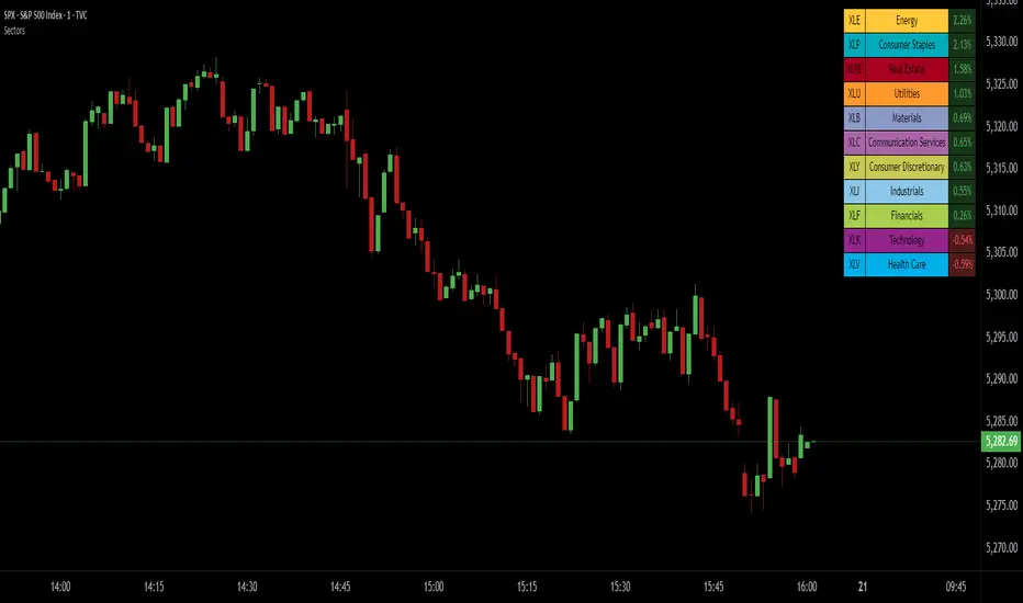
SPDR Sectors TableThis script generates an interactive and customizable SPDR Sectors Table designed to monitor and analyze the performance of the 11 main sectors of the S&P 500 via sector-specific ETFs. It offers a dynamic overview of daily or periodic sector movements, making it a valuable tool for traders, analysts, and investors implementing sector rotation strategies.
█ DEFINITIONS
SPDR Sectors ETFs are exchange-traded funds managed by State Street Global Advisors, which divide the S&P 500 into the following 11 sectors:
- Communication Services (XLC)
- Consumer Discretionary (XLY)
- Consumer Staples (XLP)
- Energy (XLE)
- Financials (XLF)
- Health Care (XLV)
- Industrials (XLI)
- Materials (XLB)
- Real Estate (XLRE)
- Technology (XLK)
- Utilities (XLU)
These ETFs aim to replicate the performance of their respective sectors as defined by the Global Industry Classification Standard (GICS). The funds are periodically rebalanced to match changes in the S&P 500 composition, offering an accurate snapshot of sectoral trends.
█ INDICATOR
The table displays each sector's ticker and full name, following official GICS terminology and SPDR color coding. It also shows percentage performance, calculated daily on intraday charts or based on the selected time frame.
Users can sort the table by either percentage performance or the relative weight of each ETF in the S&P 500. The default weight values reflect data updated as of 17 April 2025, and can be manually adjusted based on the most recent sector weightings available on the official SPDR website.
Long Term Profitable Swing | AbbasA Story of a Profitable Swing Trading Strategy
Imagine you're sailing across the ocean, looking for the perfect wave to ride. Swing trading is quite similar—you're navigating the stock market, searching for the ideal moments to enter and exit trades. This strategy, created by Abbas, helps you find those waves and ride them effectively to profitable outcomes.
🌊 Finding the Perfect Wave (Entry)
Our journey begins with two simple signs that tell us a great trading opportunity is forming:
- Moving Averages: We use two lines that follow price trends—the faster one (EMA 16) reacts quickly to recent price moves, and the slower one (EMA 30) gives us a longer-term perspective. When the faster line crosses above the slower line, it's like a clear signal saying, "Hey! The wave is rising, and prices might move higher!"
- RSI Momentum: Next, we check a tool called the RSI, which measures momentum (how strongly prices are moving). If the RSI number is above 50, it means there's enough strength behind this rising wave to carry us forward.
When both signals appear together, that's our green light. It's time to jump on our surfboard and start riding this promising wave.
⚓ Safely Riding the Wave (Risk Management)
While we're riding this wave, we want to ensure we're safe from sudden surprises. To do this, we use something called the Average True Range (ATR), which measures how volatile (or bumpy) the price movements are:
- Stop-Loss: To avoid falling too hard, we set a safety line (stop-loss) 8 times the ATR below our entry price. This helps ensure we exit if the wave suddenly turns against us, protecting us from heavy losses.
- Take Profit: We also set a goal to exit the trade at 11 times the ATR above our entry. This way, we capture significant profits when the wave reaches a nice high point.
🌟 Multiple Rides, Bigger Adventures
This strategy allows us to take multiple positions simultaneously—like riding several waves at once, up to 5. Each trade we make uses only 10% of our trading capital, keeping risks manageable and giving us multiple opportunities to win big.
🗺️ Easy to Follow Settings
Here are the basic settings we use:
- Fast EMA**: 16
- Slow EMA**: 30
- RSI Length**: 9
- RSI Threshold**: 50
- ATR Length**: 21
- ATR Stop-Loss Multiplier**: 8
- ATR Take-Profit Multiplier**: 11
These settings are flexible—you can adjust them to better suit different markets or your personal trading style.
🎉 Riding the Waves of Success
This simple yet powerful swing trading approach helps you confidently enter trades, clearly know when to exit, and effectively manage your risk. It’s a reliable way to ride market waves, capture profits, and minimize losses.
Happy trading, and may you find many profitable waves to ride! 🌊✨
Please test, and take into account that it depends on taking multiple longs within the swing, and you only get to invest 25/30% of your equity.

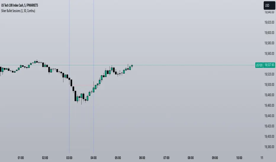
Silver Bullet SessionsThe Silver Bullet Sessions indicator is a specialized timing tool designed to highlight key market sessions throughout the trading day. By marking specific hours with vertical lines, it helps traders identify potentially significant market moments that often coincide with increased volatility and trading opportunities.
This indicator plots vertical lines at six strategic times during the trading day: 3:00 AM, 4:00 AM, 10:00 AM, 11:00 AM, 2:00 PM, and 3:00 PM. These times are carefully selected to correspond with important market events and session overlaps in the global trading cycle. The early morning hours (3-4 AM) often capture significant Asian market movements and the European market opening. The mid-morning period (10-11 AM) typically corresponds with peak European trading hours and the pre-US market dynamics. The afternoon times (2-3 PM) coincide with key US market activities and the European market close.
The indicator is implemented using Pine Script version 6, ensuring compatibility with the latest TradingView platform features. It employs a clean, efficient coding structure that minimizes resource usage while maintaining reliable performance. The vertical lines are rendered in blue for clear visibility against any chart background, and their width is optimized for easy identification without obscuring price action.
Traders can use these visual markers to:
Plan their entries and exits around these key time periods
Anticipate potential market volatility
Structure their trading sessions around these significant market hours
Identify session-based trading patterns
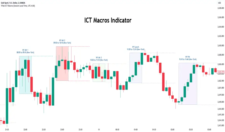
Macros ICT KillZones [TradingFinder] Times & Price Trading Setup🔵 Introduction
ICT Macros, developed by Michael Huddleston, also known as ICT (Inner Circle Trader), is a powerful trading tool designed to help traders identify the best trading opportunities during key time intervals like the London and New York trading sessions.
For traders aiming to capitalize on market volatility, liquidity shifts, and Fair Value Gaps (FVG), understanding and using these critical time zones can significantly improve trading outcomes.
In today’s highly competitive financial markets, identifying the moments when the market is seeking buy-side or sell-side liquidity, or filling price imbalances, is essential for maximizing profitability.
The ICT Macros indicator is built on the renowned ICT time and price theory, which enables traders to track and leverage key market dynamics such as breaks of highs and lows, imbalances, and liquidity hunts.
This indicator automatically detects crucial market times and optimizes strategies for traders by highlighting the specific moments when price movements are most likely to occur. A standout feature of ICT Macros is its automatic adjustment for Daylight Saving Time (DST), ensuring that traders remain synced with the correct session times.
This means you can rely on accurate market timing without the need for manual updates, allowing you to focus on capturing profitable trades during critical timeframes.
🔵 How to Use
The ICT Macros indicator helps you capitalize on trading opportunities during key market moments, particularly when the market is breaking highs or lows, filling Fair Value Gaps (FVG), or addressing imbalances. This indicator is particularly beneficial for traders who seek to identify liquidity, market volatility, and price imbalances.
🟣 Sessions
London Sessions
London Macro 1 :
UTC Time : 06:33 to 07:00
New York Time : 02:33 to 03:00
London Macro 2 :
UTC Time : 08:03 to 08:30
New York Time : 04:03 to 04:30
New York Sessions
New York Macro AM 1 :
UTC Time : 12:50 to 13:10
New York Time : 08:50 to 09:10
New York Macro AM 2 :
UTC Time : 13:50 to 14:10
New York Time : 09:50 to 10:10
New York Macro AM 3 :
UTC Time : 14:50 to 15:10
New York Time : 10:50 to 11:10
New York Lunch Macro :
UTC Time : 15:50 to 16:10
New York Time : 11:50 to 12:10
New York PM Macro :
UTC Time : 17:10 to 17:40
New York Time : 13:10 to 13:40
New York Last Hour Macro :
UTC Time : 19:15 to 19:45
New York Time : 15:15 to 15:45
These time intervals adjust automatically based on Daylight Saving Time (DST), helping traders to enter or exit trades during key market moments when price volatility is high.
Below are the main applications of this tool and how to incorporate it into your trading strategies :
🟣 Combining ICT Macros with Trading Strategies
The ICT Macros indicator can easily be used in conjunction with various trading strategies. Two well-known strategies that can be combined with this indicator include:
ICT 2022 Trading Model : This model is designed based on identifying market liquidity, structural price changes, and Fair Value Gaps (FVG). By using ICT Macros, you can identify the key time intervals when the market is seeking liquidity, filling imbalances, or breaking through important highs and lows, allowing you to enter or exit trades at the right moment.
Silver Bullet Strategy : This strategy, which is built around liquidity hunting and rapid price movements, can work more accurately with the help of ICT Macros. The indicator pinpoints precise liquidity times, helping traders take advantage of market shifts caused by filling Fair Value Gaps or correcting imbalances.
🟣 Capitalizing on Price Volatility During Key Times
Large market algorithms often seek liquidity or fill Fair Value Gaps (FVG) during the intervals marked by ICT Macros. These periods are when price volatility increases, and traders can use these moments to enter or exit trades.
For example, if sell-side liquidity is drained and the market fills an imbalance, the price might move toward buy-side liquidity. By identifying these moments, which may also involve breaking a previous high or low, you can leverage rapid market fluctuations to your advantage.
🟣 Identifying Liquidity and Price Imbalances
One of the important uses of ICT Macros is identifying points where the market is seeking liquidity and correcting imbalances. You can determine high or low liquidity levels in the market before each ICT Macro, as well as Fair Value Gaps (FVG) and price imbalances that need to be filled, using them to adjust your trading strategy. This capability allows you to manage trades based on liquidity shifts or imbalance corrections without needing a bias toward a specific direction.
🔵 Settings
The ICT Macros indicator offers various customization options, allowing users to tailor it to their specific needs. Below are the main settings:
Time Zone Mode : You can select one of the following options to define how time is displayed:
UTC : For traders who need to work with Universal Time.
Session Local Time : The local time corresponding to the London or New York markets.
Your Time Zone : You can specify your own time zone (e.g., "UTC-4:00").
Your Time Zone : If you choose "Your Time Zone," you can set your specific time zone. By default, this is set to UTC-4:00.
Show Range Time : This option allows you to display the time range of each session on the chart. If enabled, the exact start and end times of each interval are shown.
Show or Hide Time Ranges : Toggle on/off for visual clarity depending on user preference.
Custom Colors : Set distinct colors for each session, allowing users to personalize their chart based on their trading style.These settings allow you to adjust the key time intervals of each trading session to your preference and customize the time format according to your own needs.
🔵 Conclusion
The ICT Macros indicator is a powerful tool for traders, helping them to identify key time intervals where the market seeks liquidity or fills Fair Value Gaps (FVG), corrects imbalances, and breaks highs or lows. This tool is especially valuable for traders using liquidity-based strategies such as ICT 2022 or Silver Bullet.
One of the key features of this indicator is its support for Daylight Saving Time (DST), ensuring you are always in sync with the correct trading session timings without manual adjustments. This is particularly beneficial for traders operating across different time zones.
With ICT Macros, you can capitalize on crucial market opportunities during sensitive times, take advantage of imbalances, and enhance your trading strategies based on market volatility, liquidity shifts, and Fair Value Gaps.
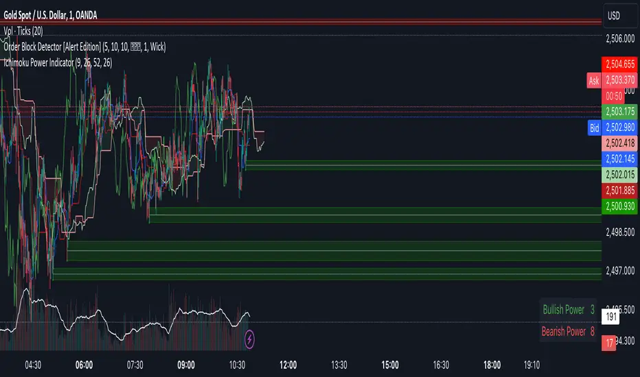
Ichimoku Power Indicator# Ichimoku Power Indicator
## Overview
The Ichimoku Power Indicator is an advanced tool that combines the traditional Ichimoku Cloud system with a unique power ranking mechanism. This indicator provides traders with a comprehensive view of market trends and potential reversal points, all while quantifying the strength of bullish and bearish signals.
## Key Features
1. **Full Ichimoku Cloud Visualization:** Displays all components of the Ichimoku Cloud system, including Conversion Line (Tenkan-sen), Base Line (Kijun-sen), Leading Span A and B (Kumo), and Lagging Span (Chikou Span).
2. **Power Ranking System:** Calculates and displays a bullish and bearish power score based on 11 different Ichimoku-derived conditions.
3. **Real-time Updates:** Power scores are updated in real-time as market conditions change.
4. **Easy-to-Read Display:** A clear, color-coded table shows the current bullish and bearish power scores.
5. **Customizable Parameters:** Allows adjustment of key Ichimoku settings to suit different trading styles and timeframes.
## How It Works
The indicator evaluates 11 different conditions derived from Ichimoku Cloud components:
1. Cloud color
2. Price position relative to the cloud
3. Tenkan-sen vs Kijun-sen
4. Price vs Tenkan-sen
5. Price vs Kijun-sen
6. Tenkan-sen vs Cloud
7. Kijun-sen vs Cloud
8. Chikou Span vs Cloud
9. Chikou Span vs Tenkan-sen
10. Chikou Span vs Kijun-sen
11. Chikou Span vs Price
Each bullish condition adds a point to the bullish power score, while each bearish condition adds a point to the bearish power score. The maximum score for each is 11.
## Interpretation
- Higher bullish scores suggest stronger upward trends or potential bullish reversals.
- Higher bearish scores indicate stronger downward trends or potential bearish reversals.
- When scores are close, it may indicate a period of consolidation or uncertainty.
## Use Cases
- Trend Confirmation: Use in conjunction with price action to confirm the strength of current trends.
- Reversal Detection: Watch for changes in power scores as early indicators of potential trend reversals.
- Entry and Exit Signals: High power scores can be used to identify optimal entry or exit points.
- Market Analysis: Gain a quick overview of market conditions across multiple assets or timeframes.
## Note
This indicator is designed to complement your existing trading strategy. Always use it in conjunction with other forms of analysis and proper risk management techniques.
Experiment with different timeframes and settings to find the configuration that best suits your trading style and the assets you trade.
Happy trading!
Daily Levels Percentual [TOLK] Settings Crypto and ForexPercentage zones refer to specific areas or bands on the price chart of a financial asset that are bounded by percentages of change relative to a reference point, such as the opening price or a reference value from a previous move.
These zones are useful for identifying support and resistance levels, predicting possible price reversals, or setting price targets. For example, on a price chart, you can create percentage zones to observe how the price behaves when it reaches 1%, 2%, 5%, 10%, etc., above or below a certain point.
These zones can be used in conjunction with other technical analysis tools, such as Fibonacci, moving averages, or volume analysis, to improve decision-making in trading strategies.
The default indicator levels are as follows:
SETTINGS Crypto:
Crypto Level 1 > 1.0%
Crypto Level 2 > 1.618%
Crypto Level 3 > 2.0%
Crypto Level 4 > 2.618%
Crypto Level 5 > 3.618%
Crypto Level 6 > 4.618%
Crypto Level 7 > 5.0%
Crypto Level 8 > 7.618%
Crypto Level 9 > 10.0%
Crypto Level 10 > 12.618%
Crypto Level 11 > 13.618%
Crypto Level 12 > 15%
Crypto Level 13 > 17.618%
Crypto Level 14 > 20%
SETTINGS Forex:
Forex Level 1 > 0.10%
Forex Level 2 > 0.1618%
Forex Level 3 > 0.20%
Forex Level 4 > 0.2618%
Forex Level 5 > 0.3618%
Forex Level 6 > 0.4618%
Forex Level 7 > 0.50%
Forex Level 8 > 0.7618%
Forex Level 9 > 1.0%
Forex Level 10 > 1.2618%
Forex Level 11 > 1.3618%
Forex Level 12 > 1.50%
Forex Level 13 > 1.7618%
Forex Level 14 > 2.0%
Percentage Levels This approach helps identify critical price levels where the asset may encounter support or resistance, making it easier to make trading decisions based on price movement patterns.

Macro Times [Blu_Ju]About ICT Macro Times:
The Inner Circle Trader (ICT) has taught that there are certain time sessions when the Interbank Price Delivery Algorithm (IPDA) is running a macro. The macro itself could be a repricing macro, a consolidation macro, etc. - this depends on where price currently is in relation to its draw. The times the macro is active do not change however, and are always the following (in New York local time):
8:50-9:10 (premarket macro)
9:50-10:10 (AM macro 1)
10:50-11:10 (AM macro 2)
11:50-12:10 (lunch macro)
13:10-13:40 (PM macro)
15:15-15:45 (final hour macro)
Because these times are fixed, traders can anticipate a setup is likely to form in or around these sessions. Setups may involve sweeps of liquidity (highs/lows), repricing to inefficiencies (e.g., fair value gaps), breaker setups, etc. (The specific setup involved is beyond the scope of this script; this script is concerned with visually marking the time sessions only.)
About this Script:
The scope of this script is to visually identify the macro active time sessions. This script draws vertical lines to mark the start and end of the macro time sessions. Optionally, the user can use a background color for the macro session with or without the vertical lines. The user can also toggle on or off any of the macro sessions, if he or she is only interested in certain ones. The user also has the freedom to change the times of the macro sessions if he or she is interested in a different time.
What makes this script unique is that it plots the macro time sessions after midnight for each day, before the real-time bar reaches the macro times. This is advantageous to the trader, as it gives the trader a visual cue that the macro times are approaching. When watching price it is easy to lose track of time, and the purpose of this script is to help the trader maintain where price is in relation to the macro time sessions in a simple, visual way.

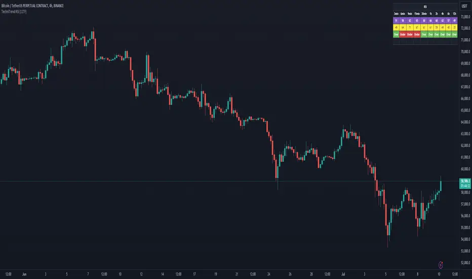
TechniTrend RSI (11TF)Multi-Timeframe RSI Indicator
Overview
The Multi-Timeframe RSI Indicator is a sophisticated tool designed to provide comprehensive insights into the Relative Strength Index (RSI) across 11 different timeframes simultaneously. This indicator is essential for traders who wish to monitor RSI trends and their moving averages (MA) to make informed trading decisions.
Features
Multiple Timeframes: Displays RSI and RSI MA values for 11 different timeframes, allowing traders to have a holistic view of the market conditions.
RSI vs. MA Comparison: Indicates whether the RSI value is above or below its moving average for each timeframe, helping traders to identify bullish or bearish momentum.
Overbought/Oversold Signals:
Marks "OS" (OverSell) when RSI falls below 25, indicating a potential oversold condition.
Marks "OB" (OverBuy) when RSI exceeds 75, signaling a potential overbought condition.
Real-Time Updates: Continuously updates in real-time to provide the most current market information.
Usage
This indicator is invaluable for traders who utilize RSI as part of their technical analysis strategy. By monitoring multiple timeframes, traders can:
Identify key overbought and oversold levels to make entry and exit decisions.
Observe the momentum shifts indicated by RSI crossing above or below its moving average.
Enhance their trading strategy by integrating multi-timeframe analysis for better accuracy and confirmation.
How to Interpret the Indicator
RSI Above MA: Indicates a potential bullish trend. Traders may consider looking for long positions.
RSI Below MA: Suggests a potential bearish trend. Traders may look for short positions.
OS (OverSell): When RSI < 25, the market may be oversold, presenting potential buying opportunities.
OB (OverBuy): When RSI > 75, the market may be overbought, indicating potential selling opportunities.
Power Hour Money StrategyDescription of the Pine Script Code: "Power Hour Money Strategy"
This Pine Script strategy, "Power Hour Money Strategy," is designed to trade based on the alignment of multiple time frames (month, week, day, and hour). The strategy aims to enter long or short positions depending on whether all selected time frames are in sync (all green for long positions, all red for short positions). Additionally, the script includes configurations for trading during specific sessions and automatically closing positions at the end of the trading day.
Core Features:
1. Time Frame Sync Check:
- The strategy evaluates whether the current price is higher than the opening price for the month, week, day, and hour to determine if each time frame is "green" (bullish) or "red" (bearish).
2. Session Control:
- The user can select between different trading sessions:
- "NY Session 9:30-11:30"
- "Extended NY Session 8-4"
- "All Sessions"
- Trades are only executed if the current time falls within the selected session.
3. Trailing Stop Mechanism:
- The strategy includes an optional trailing stop mechanism for both long and short positions.
- The trailing stop is configured with a percentage loss from the current price to protect gains.
4. End-of-Day Position Management:
- An option is provided to automatically close all positions at the end of the trading day (5:45 PM Eastern Time).
Detailed Code Breakdown:
1. Input Settings:
- **Session Selection**: Allows the user to choose the trading session.
- **End-of-Day Close**: Option to automatically close positions at the end of the day.
- **Trailing Stop Loss**: Enables or disables the trailing stop loss feature and sets the percentage for long and short positions.
2. Time Frame Calculations:
- The script uses `request.security` to get the opening prices for higher time frames (monthly, weekly, daily, and hourly).
- It compares the current close price to these opening prices to determine if each time frame is green or red.
3. Session Time Definitions:
- Defines the start and end times for the NY session (9:30-11:30 AM) and the extended session (8:00 AM - 4:00 PM).
4. Trade Execution:
- The strategy checks if all selected time frames are in sync and if the current time falls within the trading session.
- If all conditions are met, it enters a long or short position.
5. Trailing Stop Loss Implementation:
- Adjusts the stop price based on the trailing percentage and the current position's size.
- Automatically exits positions if the trailing stop condition is met.
6. End-of-Day Close Implementation:
- Uses a timestamp to check if the current time is 5:45 PM Eastern Time.
- Closes all positions if the end-of-day condition is met.
7. Plotting and Logging:
- Plots indicators to visualize the green/red status of each time frame.
- Logs information about the status of each time frame for debugging and analysis.
Example Usage:
Entering a Long Position: If the month, week, day, and hour are all green and the current time is within the selected session, a long position is entered.
Entering a Short Position: If the month, week, day, and hour are all red and the current time is within the selected session, a short position is entered.
Trailing Stop: Protects gains by exiting the position if the price moves against the set trailing stop percentage.
End-of-Day Close: Automatically closes all open positions at 5:45 PM Eastern Time if enabled.
This strategy is particularly useful for traders who want to ensure that multiple time frames are in alignment before entering a trade and who wish to manage positions effectively throughout the trading day with specific session controls and trailing stops.
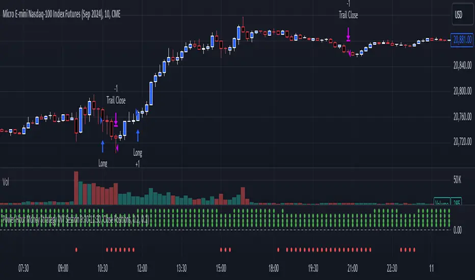
NASDAQ 100 Peak Hours StrategyNASDAQ 100 Peak Hours Trading Strategy
Description
Our NASDAQ 100 Peak Hours Trading Strategy leverages a carefully designed algorithm to trade within specific hours of high market activity, particularly focusing on the first two hours of the trading session from 09:30 AM to 11:30 AM GMT-5. This period is identified for its increased volatility and liquidity, offering numerous trading opportunities.
The strategy incorporates a blend of technical indicators to identify entry and exit points for both long and short positions. These indicators include:
Exponential Moving Averages (EMAs) : A short-term 9-period EMA and a longer-term 21-period EMA to determine the market trend and momentum.
Relative Strength Index (RSI) : A 14-period RSI to gauge the market's momentum.
Average True Range (ATR) : A 14-period ATR to assess market volatility and to set dynamic stop losses and trailing stops.
Volume Weighted Average Price (VWAP) : To identify the market's average price weighted by volume, serving as a benchmark for the trading day.
Our strategy uniquely applies a volatility filter using the ATR, ensuring trades are only executed in conditions that favor our setup. Additionally, we consider the direction of the EMAs to confirm the market's trend before entering trades.
Originality and Usefulness
This strategy stands out by combining these indicators within the NASDAQ 100's peak hours, exploiting the specific market conditions that prevail during these times. The inclusion of a volatility filter and dynamic stop-loss mechanisms based on the ATR provides a robust method for managing risk.
By focusing on the early trading hours, the strategy aims to capture the initial market movements driven by overnight news and the opening rush, often characterized by higher volatility. This approach is particularly useful for traders looking to maximize gains from short-term fluctuations while limiting exposure to longer-term market uncertainty.
Strategy Results
To ensure the strategy's effectiveness and reliability, it has undergone rigorous backtesting over a significant dataset to produce a sample size of more than 100 trades. This testing phase helps in identifying the strategy's potential in various market conditions, its consistency, and its risk-to-reward ratio.
Our backtesting adheres to realistic trading conditions, accounting for slippage and commission to reflect actual trading scenarios accurately. The strategy is designed with a conservative approach to risk management, advising not to risk more than 5-10% of equity on a single trade. The default settings in the script align with these principles, ensuring that users can replicate our tested conditions.
Using the Strategy
The strategy is designed for simplicity and ease of use:
Trade Hours : Focuses on 09:30 AM to 11:30 AM GMT-5, during the NASDAQ 100's peak activity hours.
Entry Conditions : Trades are initiated based on the alignment of EMAs, RSI, VWAP, and the ATR's volatility filter within the designated time frame.
Exit Conditions : Includes dynamic trailing stops based on ATR, a predefined time exit strategy, and a trend reversal exit condition for risk management.
This script is a powerful tool for traders looking to leverage the NASDAQ 100's peak hours, providing a structured approach to navigating the early market hours with a robust set of criteria for making informed trading decisions.

Time Based Comparison Tool [TFO]The goal of this indicator is to show how multiple assets are trading relative to their Previous Highs and Lows. Many traders have probably seen charts resembling this that may plot how asset prices are trading as a percent change over time, or something similar.
The key difference with this indicator is that all prices are normalized to reflect how they are trading with respect to the previous range of a user-defined timeframe. Without the normalization process, we would simply be observing some percent change from a given point in time; but this does not provide enough information to describe where price is trading relative to our desired frame of reference.
For example, if the timeframe setting was chosen to be 1 day, the indicator would plot the Previous High (PH) and Previous Low (PL) of the current symbol on the daily timeframe, denoted here by the black lines and labels. Then, the adjusted price of all selected symbols would be shown to visualize how each one is moving with respect its own PH and PL, using the current symbol's PH and PL as reference points.
In the above chart, we can see that CL was trading below its PDL from about 10:00-11:00 am EST, then broke above and retested it at around 11:20 am EST, before trading higher. To verify that this comparison works as intended, we can check to see that CL did in fact retest its PDL at this time before trading higher. Note that we are using the close price for this evaluation.
Since limiting the output to close prices can leave out some vital information, we can change the Plot Type setting from "Close" to "High to Low," which will instead show the range of prices from high to low instead of just the close.
We can expand on this by detecting when PH's and PL's have been raided (traded through), by displaying the text PHR (Previous High Raid) or PLR (Previous Low Raid) next to the symbol's label on the right. In this case below, where we're using the 1 week timeframe, we can observe that NQ1! (purple) traded through the PL level and thus its label (right) is updated to indicate a PLR.
Similarly, YM1! traded through its PH level and was updated to indicate a PHR; and ES1! raided both levels, with its label reflecting just that.
Due to the native limitation of output series in a single pine script, alerts have been consolidated to "Any PHR" or "Any PLR," meaning these alerts would fire if any of the selected symbols raided a PH or PL, respectively. If one wanted to be alerted for just a specific symbol, this could be achieved by deselecting all symbols except that which is desired, then setting an alert and adjusting its title for easier user recognition.

Master Fren Jedi HelperDescription:
The "Master Fren Jedi Helper" is a TradingView indicator designed to enhance trading analysis by plotting distinct lines at crucial times of the trading day.
This indicator is an invaluable tool for traders who focus on intraday price movements and patterns around specific times. Its primary features include:
Customizable Time Markers: The script allows users to mark specific times of the day with lines of different colors and styles. These times are adjustable based on the user's timezone and preferences.
Configurable Line Properties: Users can customize the color and style of each line. The script offers options for a green line at 7 AM, a red line at 11 AM, a grey line at midnight, and a yelow line to denote the daily open.
Time Zone Adjustment: To work with New York time zone, you have ability to adjust for different time zones. Users can input their time zone offset, advised to use UTC -5 allowing the script to plot the lines accurately according to their local time.
Day Labels: The indicator also labels each day of the week at midnight, providing a clear and easy way to track the days on the chart.
Functionality Overview:
Green Line at 7 AM: This line helps identify the early morning market sentiment. Users can customize the color and style of this line.
Red Line at 11 AM: Plotted to highlight mid-morning price levels, this line is also customizable in color and style.
Grey Line at Midnight: Marks the start of a new trading day. The line style and color can be personalized.
Yellow Line for Daily Open: Indicates the opening price of the day. The line's color and style are adjustable.
Time Zone Configuration: Users can set their local time zone to ensure the lines correspond accurately with their specific market hours.
Day of the Week Labels: Each midnight is labeled with the day of the week, aiding in the weekly analysis of price patterns.
This indicator is perfect for traders who need to quickly identify key times and price levels each day. It's easily configurable to suit various trading strategies and assists in enhancing the visual representation of intraday market dynamics.
Cycles 90mThe cycles are separated by vertical lines. The first cycle (Q1) is marked with a red line because it is a manipulative cycle where you should not open positions. Other cycles are green (Q2, Q3, Q4).
You can add the time of the current candle, its size and position on the chart in the settings
The time is highlighted in red in the timeframes 9:30-9:40, 10:00-10:10, 11:00-11:30, 15:30-15:40, 16:00-16:10, 17:00-17:10, 17:30-17:40, as price movements are most often expected during these timeframes.
The cycle lines automatically disappear if you open a timeframe above M15
