Simple 17 Indicator BFThis is an indicator version of my Simple 17 script.
The rules are simple, when the price closes after crossing above the MA, we have a long signal. When the price closes after crossing below the MA we have a short signal.
I have set up alerts that fire upon these crosses, one for long, one for short.
Cari dalam skrip untuk "17个交易日涨幅第一的股票(非新股)有哪些"

Simple 17 BF 🚀A Simple Moving Average of period 17 based on ohlc4 values. We go long when price closes above it. We go short when price closes below it. No stop loss. No take profit.
This strategy is really to showcase how effective a basic system can be, and that with discipline and patience, trading does not need to be complex to yield good results over time.
You can change the Moving Average type, source and period in the settings as well as the backtesting range. I found 17 period SMA with ohlc4 to be a good fit for XBT/USD on Daily timeframe but for other pairs, the type, source and period will likely differ.
INSTRUCTIONS
Red turns to Green = Long Entry/Short Exit
Green turns to Red = Short Entry/Long Exit
The entries are based on when price crosses the MA and this is what the backtest is based on. We exit the current trade when we get an opposing signal and enter the new trade.

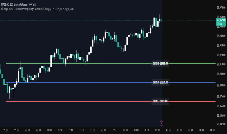
Chicago 17:00-19:00 Overnight RangeThis indicator will map out range high and range low of previous 17:00 - 19:00 of the chart. It can also display mid range if needed
Ultimate Moving Average Package (17 MA's)Included is the:
VWAP
Current time frame 10 EMA
Current time frame 20 EMA
Current time frame 50 EMA
Current time frame 10 SMA
Current time frame 20 SMA
Current time frame 50 SMA
Daily 10 EMA
Daily 20 EMA
Daily 50 EMA
Daily 50 SMA
Daily 100 SMA
Daily 200 SMA
Weekly 100 SMA
Weekly 200 SMA
Monthly 100 SMA
Monthly 200 SMA
All Daily/Weekly/Monthly MA's can be seen on intraday charts. Current time frame MA's change depending on your time frame. Obviously you dont need all 17 on your chart but you can pick the ones you like and disable the rest.


EMA72 com Difusor - Cor Dinâmica e Espessuras Ajustadas17 EMA
72 EMA (with diffuser included, green signals buy, red signals sell)
72 EMA on the weekly chart

Ichimoku Wave Oscillator with Custom MAIchimoku Wave Oscillator with Custom MA - Pine Script Description
This script uses various types of moving averages (MA) to implement the concept of Ichimoku wave theory for wave analysis. The user can select from SMA, EMA, WMA, TEMA, SMMA to visualize the difference between short-term, medium-term, and long-term waves, while identifying potential buy and sell signals at crossover points.
Key Features:
MA Type Selection:
The user can select from SMA (Simple Moving Average), EMA (Exponential Moving Average), WMA (Weighted Moving Average), TEMA (Triple Exponential Moving Average), and SMMA (Smoothed Moving Average) to calculate the waves. This script is unique in that it combines TEMA and SMMA, distinguishing it from other simple moving average-based indicators.
TEMA (Triple Exponential Moving Average): Best suited for capturing short-term trends with quick responsiveness.
SMMA (Smoothed Moving Average): Useful for identifying long-term trends with minimal noise, providing more stable signals.
Wave Calculations:
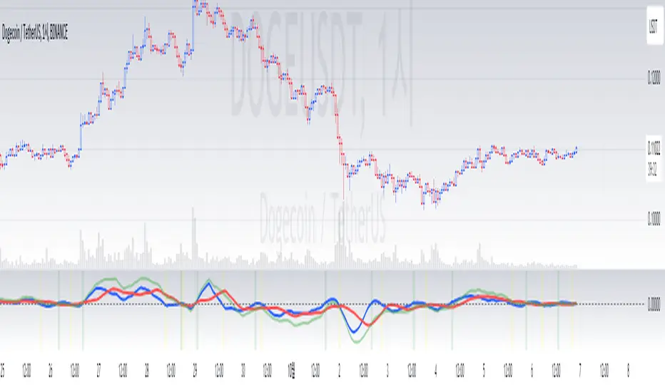
The script calculates three waves: Wave 9-17, Wave 17-26, and Wave 9-26, each of which analyzes different time horizons.
Wave 9-17 (blue): Primarily used for analyzing short-term trends, ideal for detecting quick changes.
Wave 17-26 (red): Used to analyze medium-term trends, providing a more stable market direction.
Wave 9-26 (green): Represents long-term trends, suitable for understanding broader trend shifts.
Baseline (0 Line):
Each wave is visualized around the 0 line, where waves above the line indicate an uptrend and waves below the line indicate a downtrend. This allows for easy identification of trend reversals.
Crossover Signals:
CrossUp: When Wave 9-17 (short-term wave) crosses Wave 17-26 (medium-term wave) upward, it is considered a buy signal, indicating a potential upward trend shift.
CrossDown: When Wave 9-17 (short-term wave) crosses Wave 17-26 downward, it is considered a sell signal, indicating a potential downward trend shift.
Background Color for Signal:
The script visually highlights the signals with background colors. When a buy signal occurs, the background turns green, and when a sell signal occurs, the background turns red. This makes it easier to spot reversal points.
Calculation Method:
The script calculates the difference between moving averages to display the wave oscillation. Wave 9-17, Wave 17-26, and Wave 9-26 represent the difference between the moving averages for different time periods, allowing for analysis of short-term, medium-term, and long-term trends.
Wave 9-17 = MA(9) - MA(17): Represents the difference between the short-term moving averages.
Wave 17-26 = MA(17) - MA(26): Represents the difference between medium-term moving averages.
Wave 9-26 = MA(9) - MA(26): Provides insight into the long-term trend.
This calculation method effectively visualizes the oscillation of waves and helps identify trend reversals at crossover points.
Uniqueness of the Script:
Unlike other moving average-based indicators, this script combines TEMA (Triple Exponential Moving Average) and SMMA (Smoothed Moving Average) to capture both short-term sensitivity and long-term stability in trends. This duality makes the script more versatile for different market conditions.
TEMA is ideal for short-term traders who need quick signals, while SMMA is useful for long-term investors seeking stability and noise reduction. By combining these two, this script provides a more refined analysis of trend changes across various timeframes.
How to Use:
This script is effective for trend analysis and reversal detection. By visualizing the crossover points between the waves, users can spot potential buy and sell signals to make more informed trading decisions.
Scalping strategies can rely on Wave 9-17 to detect quick trend changes, while those looking for medium-term trends can analyze signals from Wave 17-26.
For a broader market overview, Wave 9-26 helps users understand the long-term market trend.
This script is built on the concept of wave theory to anticipate trend changes, making it suitable for various timeframes and strategies. The user can tailor the characteristics of the waves by selecting different MA types, allowing for flexible application across different trading strategies.
Ichimoku Wave Oscillator with Custom MA - Pine Script 설명
이 스크립트는 다양한 이동 평균(MA) 유형을 활용하여 일목 파동론의 개념을 기반으로 파동 분석을 시도하는 지표입니다. 사용자는 SMA, EMA, WMA, TEMA, SMMA 중 원하는 이동 평균을 선택할 수 있으며, 이를 통해 단기, 중기, 장기 파동 간의 차이를 시각화하고, 교차점에서 상승 및 하락 신호를 포착할 수 있습니다.
주요 기능:
이동 평균(MA) 유형 선택:
사용자는 SMA(단순 이동 평균), EMA(지수 이동 평균), WMA(가중 이동 평균), TEMA(삼중 지수 이동 평균), SMMA(평활 이동 평균) 중 하나를 선택하여 파동을 계산할 수 있습니다. 이 스크립트는 TEMA와 SMMA의 독창적인 조합을 통해 기존의 단순한 이동 평균 지표와 차별화됩니다.
TEMA(삼중 지수 이동 평균): 빠른 반응으로 단기 트렌드를 포착하는 데 적합합니다.
SMMA(평활 이동 평균): 장기적인 추세를 파악하는 데 유용하며, 노이즈를 최소화하여 안정적인 신호를 제공합니다.
파동(Wave) 계산:
이 스크립트는 Wave 9-17, Wave 17-26, Wave 9-26의 세 가지 파동을 계산하여 각각 단기, 중기, 장기 추세를 분석합니다.
Wave 9-17 (파란색): 주로 단기 추세를 분석하는 데 사용되며, 빠른 추세 변화를 포착하는 데 유용합니다.
Wave 17-26 (빨간색): 중기 추세를 분석하는 데 사용되며, 좀 더 안정적인 시장 흐름을 보여줍니다.
Wave 9-26 (녹색): 장기 추세를 나타내며, 큰 흐름의 방향성을 파악하는 데 적합합니다.
기준선(0 라인):
각 파동은 0 라인을 기준으로 변동성을 시각화합니다. 0 위에 있는 파동은 상승세, 0 아래에 있는 파동은 하락세를 나타내며, 이를 통해 추세의 전환을 쉽게 확인할 수 있습니다.
파동 교차 신호:
CrossUp: Wave 9-17(단기 파동)이 Wave 17-26(중기 파동)을 상향 교차할 때, 상승 신호로 간주됩니다. 이는 단기적인 추세 변화가 발생할 수 있음을 의미합니다.
CrossDown: Wave 9-17(단기 파동)이 Wave 17-26(중기 파동)을 하향 교차할 때, 하락 신호로 해석됩니다. 이는 시장이 약세로 돌아설 가능성을 나타냅니다.
배경 색상 표시:
교차 신호가 발생할 때, 상승 신호는 녹색 배경, 하락 신호는 빨간색 배경으로 시각적으로 강조되어 사용자가 신호를 쉽게 인식할 수 있습니다.
계산 방식:
이 스크립트는 이동 평균 간의 차이를 계산하여 각 파동의 변동성을 나타냅니다. Wave 9-17, Wave 17-26, Wave 9-26은 각각 설정된 주기의 이동 평균(MA)의 차이를 통해, 시장의 단기, 중기, 장기 추세 변화를 시각적으로 표현합니다.
Wave 9-17 = MA(9) - MA(17): 단기 추세의 차이를 나타냅니다.
Wave 17-26 = MA(17) - MA(26): 중기 추세의 차이를 나타냅니다.
Wave 9-26 = MA(9) - MA(26): 장기적인 추세 방향을 파악할 수 있습니다.
이러한 계산 방식은 파동의 변동성을 파악하는 데 유용하며, 추세의 교차점을 통해 상승/하락 신호를 잡아냅니다.
스크립트의 독창성:
이 스크립트는 기존의 이동 평균 기반 지표들과 달리, TEMA(삼중 지수 이동 평균)와 SMMA(평활 이동 평균)을 함께 사용하여 짧은 주기와 긴 주기의 트렌드를 동시에 파악할 수 있도록 설계되었습니다. 이를 통해 단기 트렌드의 민감한 변화와 장기 트렌드의 안정성을 모두 반영합니다.
TEMA는 단기 트레이더에게 빠르고 민첩한 신호를 제공하며, SMMA는 장기 투자자에게 보다 안정적이고 긴 호흡의 트렌드를 파악하는 데 유리합니다. 두 지표의 결합으로, 다양한 시장 환경에서 추세의 변화를 더 정교하게 분석할 수 있습니다.
사용 방법:
이 스크립트는 추세 분석과 변곡점 포착에 효과적입니다. 각 파동 간의 교차점을 시각적으로 확인하고, 상승 또는 하락 신호를 포착하여 매매 시점 결정을 도울 수 있습니다.
스캘핑 전략에서는 Wave 9-17을 주로 참고하여 빠르게 추세 변화를 잡아내고, 중기 추세를 참고하고 싶은 경우 Wave 17-26을 사용해 신호를 분석할 수 있습니다.
장기적인 시장 흐름을 파악하고자 할 때는 Wave 9-26을 통해 큰 트렌드를 확인할 수 있습니다.
이 스크립트는 파동 이론의 개념을 기반으로 시장의 추세 변화를 예측하는 데 유용하며, 다양한 시간대와 전략에 맞추어 사용할 수 있습니다. 특히, 사용자가 선택한 MA 유형에 따라 파동의 특성을 변화시킬 수 있어, 여러 매매 전략에 유연하게 대응할 수 있습니다.
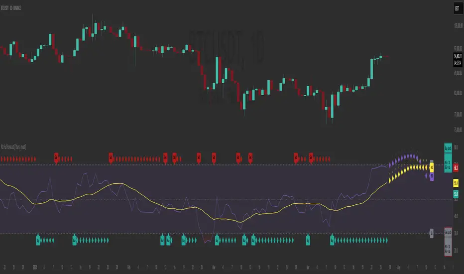
RSI Full Forecast [Titans_Invest]RSI Full Forecast
Get ready to experience the ultimate evolution of RSI-based indicators – the RSI Full Forecast, a boosted and even smarter version of the already powerful: RSI Forecast
Now featuring over 40 additional entry conditions (forecasts), this indicator redefines the way you view the market.
AI-Powered RSI Forecasting:
Using advanced linear regression with the least squares method – a solid foundation for machine learning - the RSI Full Forecast enables you to predict future RSI behavior with impressive accuracy.
But that’s not all: this new version also lets you monitor future crossovers between the RSI and the MA RSI, delivering early and strategic signals that go far beyond traditional analysis.
You’ll be able to monitor future crossovers up to 20 bars ahead, giving you an even broader and more precise view of market movements.
See the Future, Now:
• Track upcoming RSI & RSI MA crossovers in advance.
• Identify potential reversal zones before price reacts.
• Uncover statistical behavior patterns that would normally go unnoticed.
40+ Intelligent Conditions:
The new layer of conditions is designed to detect multiple high-probability scenarios based on historical patterns and predictive modeling. Each additional forecast is a window into the price's future, powered by robust mathematics and advanced algorithmic logic.
Full Customization:
All parameters can be tailored to fit your strategy – from smoothing periods to prediction sensitivity. You have complete control to turn raw data into smart decisions.
Innovative, Accurate, Unique:
This isn’t just an upgrade. It’s a quantum leap in technical analysis.
RSI Full Forecast is the first of its kind: an indicator that blends statistical analysis, machine learning, and visual design to create a true real-time predictive system.
⯁ SCIENTIFIC BASIS LINEAR REGRESSION
Linear Regression is a fundamental method of statistics and machine learning, used to model the relationship between a dependent variable y and one or more independent variables 𝑥.
The general formula for a simple linear regression is given by:
y = β₀ + β₁x + ε
β₁ = Σ((xᵢ - x̄)(yᵢ - ȳ)) / Σ((xᵢ - x̄)²)
β₀ = ȳ - β₁x̄
Where:
y = is the predicted variable (e.g. future value of RSI)
x = is the explanatory variable (e.g. time or bar index)
β0 = is the intercept (value of 𝑦 when 𝑥 = 0)
𝛽1 = is the slope of the line (rate of change)
ε = is the random error term
The goal is to estimate the coefficients 𝛽0 and 𝛽1 so as to minimize the sum of the squared errors — the so-called Random Error Method Least Squares.
⯁ LEAST SQUARES ESTIMATION
To minimize the error between predicted and observed values, we use the following formulas:
β₁ = /
β₀ = ȳ - β₁x̄
Where:
∑ = sum
x̄ = mean of x
ȳ = mean of y
x_i, y_i = individual values of the variables.
Where:
x_i and y_i are the means of the independent and dependent variables, respectively.
i ranges from 1 to n, the number of observations.
These equations guarantee the best linear unbiased estimator, according to the Gauss-Markov theorem, assuming homoscedasticity and linearity.
⯁ LINEAR REGRESSION IN MACHINE LEARNING
Linear regression is one of the cornerstones of supervised learning. Its simplicity and ability to generate accurate quantitative predictions make it essential in AI systems, predictive algorithms, time series analysis, and automated trading strategies.
By applying this model to the RSI, you are literally putting artificial intelligence at the heart of a classic indicator, bringing a new dimension to technical analysis.
⯁ VISUAL INTERPRETATION
Imagine an RSI time series like this:
Time →
RSI →
The regression line will smooth these values and extend them n periods into the future, creating a predicted trajectory based on the historical moment. This line becomes the predicted RSI, which can be crossed with the actual RSI to generate more intelligent signals.
⯁ SUMMARY OF SCIENTIFIC CONCEPTS USED
Linear Regression Models the relationship between variables using a straight line.
Least Squares Minimizes the sum of squared errors between prediction and reality.
Time Series Forecasting Estimates future values based on historical data.
Supervised Learning Trains models to predict outputs from known inputs.
Statistical Smoothing Reduces noise and reveals underlying trends.
⯁ WHY THIS INDICATOR IS REVOLUTIONARY
Scientifically-based: Based on statistical theory and mathematical inference.
Unprecedented: First public RSI with least squares predictive modeling.
Intelligent: Built with machine learning logic.
Practical: Generates forward-thinking signals.
Customizable: Flexible for any trading strategy.
⯁ CONCLUSION
By combining RSI with linear regression, this indicator allows a trader to predict market momentum, not just follow it.
RSI Full Forecast is not just an indicator — it is a scientific breakthrough in technical analysis technology.
⯁ Example of simple linear regression, which has one independent variable:
⯁ In linear regression, observations ( red ) are considered to be the result of random deviations ( green ) from an underlying relationship ( blue ) between a dependent variable ( y ) and an independent variable ( x ).
⯁ Visualizing heteroscedasticity in a scatterplot against 100 random fitted values using Matlab:
⯁ The data sets in the Anscombe's quartet are designed to have approximately the same linear regression line (as well as nearly identical means, standard deviations, and correlations) but are graphically very different. This illustrates the pitfalls of relying solely on a fitted model to understand the relationship between variables.
⯁ The result of fitting a set of data points with a quadratic function:
_________________________________________________
🔮 Linear Regression: PineScript Technical Parameters 🔮
_________________________________________________
Forecast Types:
• Flat: Assumes prices will remain the same.
• Linreg: Makes a 'Linear Regression' forecast for n periods.
Technical Information:
ta.linreg (built-in function)
Linear regression curve. A line that best fits the specified prices over a user-defined time period. It is calculated using the least squares method. The result of this function is calculated using the formula: linreg = intercept + slope * (length - 1 - offset), where intercept and slope are the values calculated using the least squares method on the source series.
Syntax:
• Function: ta.linreg()
Parameters:
• source: Source price series.
• length: Number of bars (period).
• offset: Offset.
• return: Linear regression curve.
This function has been cleverly applied to the RSI, making it capable of projecting future values based on past statistical trends.
______________________________________________________
______________________________________________________
⯁ WHAT IS THE RSI❓
The Relative Strength Index (RSI) is a technical analysis indicator developed by J. Welles Wilder. It measures the magnitude of recent price movements to evaluate overbought or oversold conditions in a market. The RSI is an oscillator that ranges from 0 to 100 and is commonly used to identify potential reversal points, as well as the strength of a trend.
⯁ HOW TO USE THE RSI❓
The RSI is calculated based on average gains and losses over a specified period (usually 14 periods). It is plotted on a scale from 0 to 100 and includes three main zones:
• Overbought: When the RSI is above 70, indicating that the asset may be overbought.
• Oversold: When the RSI is below 30, indicating that the asset may be oversold.
• Neutral Zone: Between 30 and 70, where there is no clear signal of overbought or oversold conditions.
______________________________________________________
______________________________________________________
⯁ ENTRY CONDITIONS
The conditions below are fully flexible and allow for complete customization of the signal.
______________________________________________________
______________________________________________________
🔹 CONDITIONS TO BUY 📈
______________________________________________________
• Signal Validity: The signal will remain valid for X bars .
• Signal Sequence: Configurable as AND or OR .
📈 RSI Conditions:
🔹 RSI > Upper
🔹 RSI < Upper
🔹 RSI > Lower
🔹 RSI < Lower
🔹 RSI > Middle
🔹 RSI < Middle
🔹 RSI > MA
🔹 RSI < MA
📈 MA Conditions:
🔹 MA > Upper
🔹 MA < Upper
🔹 MA > Lower
🔹 MA < Lower
📈 Crossovers:
🔹 RSI (Crossover) Upper
🔹 RSI (Crossunder) Upper
🔹 RSI (Crossover) Lower
🔹 RSI (Crossunder) Lower
🔹 RSI (Crossover) Middle
🔹 RSI (Crossunder) Middle
🔹 RSI (Crossover) MA
🔹 RSI (Crossunder) MA
🔹 MA (Crossover) Upper
🔹 MA (Crossunder) Upper
🔹 MA (Crossover) Lower
🔹 MA (Crossunder) Lower
📈 RSI Divergences:
🔹 RSI Divergence Bull
🔹 RSI Divergence Bear
📈 RSI Forecast:
🔹 RSI (Crossover) MA Forecast
🔹 RSI (Crossunder) MA Forecast
🔹 RSI Forecast 1 > MA Forecast 1
🔹 RSI Forecast 1 < MA Forecast 1
🔹 RSI Forecast 2 > MA Forecast 2
🔹 RSI Forecast 2 < MA Forecast 2
🔹 RSI Forecast 3 > MA Forecast 3
🔹 RSI Forecast 3 < MA Forecast 3
🔹 RSI Forecast 4 > MA Forecast 4
🔹 RSI Forecast 4 < MA Forecast 4
🔹 RSI Forecast 5 > MA Forecast 5
🔹 RSI Forecast 5 < MA Forecast 5
🔹 RSI Forecast 6 > MA Forecast 6
🔹 RSI Forecast 6 < MA Forecast 6
🔹 RSI Forecast 7 > MA Forecast 7
🔹 RSI Forecast 7 < MA Forecast 7
🔹 RSI Forecast 8 > MA Forecast 8
🔹 RSI Forecast 8 < MA Forecast 8
🔹 RSI Forecast 9 > MA Forecast 9
🔹 RSI Forecast 9 < MA Forecast 9
🔹 RSI Forecast 10 > MA Forecast 10
🔹 RSI Forecast 10 < MA Forecast 10
🔹 RSI Forecast 11 > MA Forecast 11
🔹 RSI Forecast 11 < MA Forecast 11
🔹 RSI Forecast 12 > MA Forecast 12
🔹 RSI Forecast 12 < MA Forecast 12
🔹 RSI Forecast 13 > MA Forecast 13
🔹 RSI Forecast 13 < MA Forecast 13
🔹 RSI Forecast 14 > MA Forecast 14
🔹 RSI Forecast 14 < MA Forecast 14
🔹 RSI Forecast 15 > MA Forecast 15
🔹 RSI Forecast 15 < MA Forecast 15
🔹 RSI Forecast 16 > MA Forecast 16
🔹 RSI Forecast 16 < MA Forecast 16
🔹 RSI Forecast 17 > MA Forecast 17
🔹 RSI Forecast 17 < MA Forecast 17
🔹 RSI Forecast 18 > MA Forecast 18
🔹 RSI Forecast 18 < MA Forecast 18
🔹 RSI Forecast 19 > MA Forecast 19
🔹 RSI Forecast 19 < MA Forecast 19
🔹 RSI Forecast 20 > MA Forecast 20
🔹 RSI Forecast 20 < MA Forecast 20
______________________________________________________
______________________________________________________
🔸 CONDITIONS TO SELL 📉
______________________________________________________
• Signal Validity: The signal will remain valid for X bars .
• Signal Sequence: Configurable as AND or OR .
📉 RSI Conditions:
🔸 RSI > Upper
🔸 RSI < Upper
🔸 RSI > Lower
🔸 RSI < Lower
🔸 RSI > Middle
🔸 RSI < Middle
🔸 RSI > MA
🔸 RSI < MA
📉 MA Conditions:
🔸 MA > Upper
🔸 MA < Upper
🔸 MA > Lower
🔸 MA < Lower
📉 Crossovers:
🔸 RSI (Crossover) Upper
🔸 RSI (Crossunder) Upper
🔸 RSI (Crossover) Lower
🔸 RSI (Crossunder) Lower
🔸 RSI (Crossover) Middle
🔸 RSI (Crossunder) Middle
🔸 RSI (Crossover) MA
🔸 RSI (Crossunder) MA
🔸 MA (Crossover) Upper
🔸 MA (Crossunder) Upper
🔸 MA (Crossover) Lower
🔸 MA (Crossunder) Lower
📉 RSI Divergences:
🔸 RSI Divergence Bull
🔸 RSI Divergence Bear
📉 RSI Forecast:
🔸 RSI (Crossover) MA Forecast
🔸 RSI (Crossunder) MA Forecast
🔸 RSI Forecast 1 > MA Forecast 1
🔸 RSI Forecast 1 < MA Forecast 1
🔸 RSI Forecast 2 > MA Forecast 2
🔸 RSI Forecast 2 < MA Forecast 2
🔸 RSI Forecast 3 > MA Forecast 3
🔸 RSI Forecast 3 < MA Forecast 3
🔸 RSI Forecast 4 > MA Forecast 4
🔸 RSI Forecast 4 < MA Forecast 4
🔸 RSI Forecast 5 > MA Forecast 5
🔸 RSI Forecast 5 < MA Forecast 5
🔸 RSI Forecast 6 > MA Forecast 6
🔸 RSI Forecast 6 < MA Forecast 6
🔸 RSI Forecast 7 > MA Forecast 7
🔸 RSI Forecast 7 < MA Forecast 7
🔸 RSI Forecast 8 > MA Forecast 8
🔸 RSI Forecast 8 < MA Forecast 8
🔸 RSI Forecast 9 > MA Forecast 9
🔸 RSI Forecast 9 < MA Forecast 9
🔸 RSI Forecast 10 > MA Forecast 10
🔸 RSI Forecast 10 < MA Forecast 10
🔸 RSI Forecast 11 > MA Forecast 11
🔸 RSI Forecast 11 < MA Forecast 11
🔸 RSI Forecast 12 > MA Forecast 12
🔸 RSI Forecast 12 < MA Forecast 12
🔸 RSI Forecast 13 > MA Forecast 13
🔸 RSI Forecast 13 < MA Forecast 13
🔸 RSI Forecast 14 > MA Forecast 14
🔸 RSI Forecast 14 < MA Forecast 14
🔸 RSI Forecast 15 > MA Forecast 15
🔸 RSI Forecast 15 < MA Forecast 15
🔸 RSI Forecast 16 > MA Forecast 16
🔸 RSI Forecast 16 < MA Forecast 16
🔸 RSI Forecast 17 > MA Forecast 17
🔸 RSI Forecast 17 < MA Forecast 17
🔸 RSI Forecast 18 > MA Forecast 18
🔸 RSI Forecast 18 < MA Forecast 18
🔸 RSI Forecast 19 > MA Forecast 19
🔸 RSI Forecast 19 < MA Forecast 19
🔸 RSI Forecast 20 > MA Forecast 20
🔸 RSI Forecast 20 < MA Forecast 20
______________________________________________________
______________________________________________________
🤖 AUTOMATION 🤖
• You can automate the BUY and SELL signals of this indicator.
______________________________________________________
______________________________________________________
⯁ UNIQUE FEATURES
______________________________________________________
Linear Regression: (Forecast)
Signal Validity: The signal will remain valid for X bars
Signal Sequence: Configurable as AND/OR
Condition Table: BUY/SELL
Condition Labels: BUY/SELL
Plot Labels in the Graph Above: BUY/SELL
Automate and Monitor Signals/Alerts: BUY/SELL
Linear Regression (Forecast)
Signal Validity: The signal will remain valid for X bars
Signal Sequence: Configurable as AND/OR
Condition Table: BUY/SELL
Condition Labels: BUY/SELL
Plot Labels in the Graph Above: BUY/SELL
Automate and Monitor Signals/Alerts: BUY/SELL
______________________________________________________
📜 SCRIPT : RSI Full Forecast
🎴 Art by : @Titans_Invest & @DiFlip
👨💻 Dev by : @Titans_Invest & @DiFlip
🎑 Titans Invest — The Wizards Without Gloves 🧤
✨ Enjoy!
______________________________________________________
o Mission 🗺
• Inspire Traders to manifest Magic in the Market.
o Vision 𐓏
• To elevate collective Energy 𐓷𐓏
PubLibCandleTrendLibrary "PubLibCandleTrend"
candle trend, multi-part candle trend, multi-part green/red candle trend, double candle trend and multi-part double candle trend conditions for indicator and strategy development
chh()
candle higher high condition
Returns: bool
chl()
candle higher low condition
Returns: bool
clh()
candle lower high condition
Returns: bool
cll()
candle lower low condition
Returns: bool
cdt()
candle double top condition
Returns: bool
cdb()
candle double bottom condition
Returns: bool
gc()
green candle condition
Returns: bool
gchh()
green candle higher high condition
Returns: bool
gchl()
green candle higher low condition
Returns: bool
gclh()
green candle lower high condition
Returns: bool
gcll()
green candle lower low condition
Returns: bool
gcdt()
green candle double top condition
Returns: bool
gcdb()
green candle double bottom condition
Returns: bool
rc()
red candle condition
Returns: bool
rchh()
red candle higher high condition
Returns: bool
rchl()
red candle higher low condition
Returns: bool
rclh()
red candle lower high condition
Returns: bool
rcll()
red candle lower low condition
Returns: bool
rcdt()
red candle double top condition
Returns: bool
rcdb()
red candle double bottom condition
Returns: bool
chh_1p()
1-part candle higher high condition
Returns: bool
chh_2p()
2-part candle higher high condition
Returns: bool
chh_3p()
3-part candle higher high condition
Returns: bool
chh_4p()
4-part candle higher high condition
Returns: bool
chh_5p()
5-part candle higher high condition
Returns: bool
chh_6p()
6-part candle higher high condition
Returns: bool
chh_7p()
7-part candle higher high condition
Returns: bool
chh_8p()
8-part candle higher high condition
Returns: bool
chh_9p()
9-part candle higher high condition
Returns: bool
chh_10p()
10-part candle higher high condition
Returns: bool
chh_11p()
11-part candle higher high condition
Returns: bool
chh_12p()
12-part candle higher high condition
Returns: bool
chh_13p()
13-part candle higher high condition
Returns: bool
chh_14p()
14-part candle higher high condition
Returns: bool
chh_15p()
15-part candle higher high condition
Returns: bool
chh_16p()
16-part candle higher high condition
Returns: bool
chh_17p()
17-part candle higher high condition
Returns: bool
chh_18p()
18-part candle higher high condition
Returns: bool
chh_19p()
19-part candle higher high condition
Returns: bool
chh_20p()
20-part candle higher high condition
Returns: bool
chh_21p()
21-part candle higher high condition
Returns: bool
chh_22p()
22-part candle higher high condition
Returns: bool
chh_23p()
23-part candle higher high condition
Returns: bool
chh_24p()
24-part candle higher high condition
Returns: bool
chh_25p()
25-part candle higher high condition
Returns: bool
chh_26p()
26-part candle higher high condition
Returns: bool
chh_27p()
27-part candle higher high condition
Returns: bool
chh_28p()
28-part candle higher high condition
Returns: bool
chh_29p()
29-part candle higher high condition
Returns: bool
chh_30p()
30-part candle higher high condition
Returns: bool
chl_1p()
1-part candle higher low condition
Returns: bool
chl_2p()
2-part candle higher low condition
Returns: bool
chl_3p()
3-part candle higher low condition
Returns: bool
chl_4p()
4-part candle higher low condition
Returns: bool
chl_5p()
5-part candle higher low condition
Returns: bool
chl_6p()
6-part candle higher low condition
Returns: bool
chl_7p()
7-part candle higher low condition
Returns: bool
chl_8p()
8-part candle higher low condition
Returns: bool
chl_9p()
9-part candle higher low condition
Returns: bool
chl_10p()
10-part candle higher low condition
Returns: bool
chl_11p()
11-part candle higher low condition
Returns: bool
chl_12p()
12-part candle higher low condition
Returns: bool
chl_13p()
13-part candle higher low condition
Returns: bool
chl_14p()
14-part candle higher low condition
Returns: bool
chl_15p()
15-part candle higher low condition
Returns: bool
chl_16p()
16-part candle higher low condition
Returns: bool
chl_17p()
17-part candle higher low condition
Returns: bool
chl_18p()
18-part candle higher low condition
Returns: bool
chl_19p()
19-part candle higher low condition
Returns: bool
chl_20p()
20-part candle higher low condition
Returns: bool
chl_21p()
21-part candle higher low condition
Returns: bool
chl_22p()
22-part candle higher low condition
Returns: bool
chl_23p()
23-part candle higher low condition
Returns: bool
chl_24p()
24-part candle higher low condition
Returns: bool
chl_25p()
25-part candle higher low condition
Returns: bool
chl_26p()
26-part candle higher low condition
Returns: bool
chl_27p()
27-part candle higher low condition
Returns: bool
chl_28p()
28-part candle higher low condition
Returns: bool
chl_29p()
29-part candle higher low condition
Returns: bool
chl_30p()
30-part candle higher low condition
Returns: bool
clh_1p()
1-part candle lower high condition
Returns: bool
clh_2p()
2-part candle lower high condition
Returns: bool
clh_3p()
3-part candle lower high condition
Returns: bool
clh_4p()
4-part candle lower high condition
Returns: bool
clh_5p()
5-part candle lower high condition
Returns: bool
clh_6p()
6-part candle lower high condition
Returns: bool
clh_7p()
7-part candle lower high condition
Returns: bool
clh_8p()
8-part candle lower high condition
Returns: bool
clh_9p()
9-part candle lower high condition
Returns: bool
clh_10p()
10-part candle lower high condition
Returns: bool
clh_11p()
11-part candle lower high condition
Returns: bool
clh_12p()
12-part candle lower high condition
Returns: bool
clh_13p()
13-part candle lower high condition
Returns: bool
clh_14p()
14-part candle lower high condition
Returns: bool
clh_15p()
15-part candle lower high condition
Returns: bool
clh_16p()
16-part candle lower high condition
Returns: bool
clh_17p()
17-part candle lower high condition
Returns: bool
clh_18p()
18-part candle lower high condition
Returns: bool
clh_19p()
19-part candle lower high condition
Returns: bool
clh_20p()
20-part candle lower high condition
Returns: bool
clh_21p()
21-part candle lower high condition
Returns: bool
clh_22p()
22-part candle lower high condition
Returns: bool
clh_23p()
23-part candle lower high condition
Returns: bool
clh_24p()
24-part candle lower high condition
Returns: bool
clh_25p()
25-part candle lower high condition
Returns: bool
clh_26p()
26-part candle lower high condition
Returns: bool
clh_27p()
27-part candle lower high condition
Returns: bool
clh_28p()
28-part candle lower high condition
Returns: bool
clh_29p()
29-part candle lower high condition
Returns: bool
clh_30p()
30-part candle lower high condition
Returns: bool
cll_1p()
1-part candle lower low condition
Returns: bool
cll_2p()
2-part candle lower low condition
Returns: bool
cll_3p()
3-part candle lower low condition
Returns: bool
cll_4p()
4-part candle lower low condition
Returns: bool
cll_5p()
5-part candle lower low condition
Returns: bool
cll_6p()
6-part candle lower low condition
Returns: bool
cll_7p()
7-part candle lower low condition
Returns: bool
cll_8p()
8-part candle lower low condition
Returns: bool
cll_9p()
9-part candle lower low condition
Returns: bool
cll_10p()
10-part candle lower low condition
Returns: bool
cll_11p()
11-part candle lower low condition
Returns: bool
cll_12p()
12-part candle lower low condition
Returns: bool
cll_13p()
13-part candle lower low condition
Returns: bool
cll_14p()
14-part candle lower low condition
Returns: bool
cll_15p()
15-part candle lower low condition
Returns: bool
cll_16p()
16-part candle lower low condition
Returns: bool
cll_17p()
17-part candle lower low condition
Returns: bool
cll_18p()
18-part candle lower low condition
Returns: bool
cll_19p()
19-part candle lower low condition
Returns: bool
cll_20p()
20-part candle lower low condition
Returns: bool
cll_21p()
21-part candle lower low condition
Returns: bool
cll_22p()
22-part candle lower low condition
Returns: bool
cll_23p()
23-part candle lower low condition
Returns: bool
cll_24p()
24-part candle lower low condition
Returns: bool
cll_25p()
25-part candle lower low condition
Returns: bool
cll_26p()
26-part candle lower low condition
Returns: bool
cll_27p()
27-part candle lower low condition
Returns: bool
cll_28p()
28-part candle lower low condition
Returns: bool
cll_29p()
29-part candle lower low condition
Returns: bool
cll_30p()
30-part candle lower low condition
Returns: bool
gc_1p()
1-part green candle condition
Returns: bool
gc_2p()
2-part green candle condition
Returns: bool
gc_3p()
3-part green candle condition
Returns: bool
gc_4p()
4-part green candle condition
Returns: bool
gc_5p()
5-part green candle condition
Returns: bool
gc_6p()
6-part green candle condition
Returns: bool
gc_7p()
7-part green candle condition
Returns: bool
gc_8p()
8-part green candle condition
Returns: bool
gc_9p()
9-part green candle condition
Returns: bool
gc_10p()
10-part green candle condition
Returns: bool
gc_11p()
11-part green candle condition
Returns: bool
gc_12p()
12-part green candle condition
Returns: bool
gc_13p()
13-part green candle condition
Returns: bool
gc_14p()
14-part green candle condition
Returns: bool
gc_15p()
15-part green candle condition
Returns: bool
gc_16p()
16-part green candle condition
Returns: bool
gc_17p()
17-part green candle condition
Returns: bool
gc_18p()
18-part green candle condition
Returns: bool
gc_19p()
19-part green candle condition
Returns: bool
gc_20p()
20-part green candle condition
Returns: bool
gc_21p()
21-part green candle condition
Returns: bool
gc_22p()
22-part green candle condition
Returns: bool
gc_23p()
23-part green candle condition
Returns: bool
gc_24p()
24-part green candle condition
Returns: bool
gc_25p()
25-part green candle condition
Returns: bool
gc_26p()
26-part green candle condition
Returns: bool
gc_27p()
27-part green candle condition
Returns: bool
gc_28p()
28-part green candle condition
Returns: bool
gc_29p()
29-part green candle condition
Returns: bool
gc_30p()
30-part green candle condition
Returns: bool
rc_1p()
1-part red candle condition
Returns: bool
rc_2p()
2-part red candle condition
Returns: bool
rc_3p()
3-part red candle condition
Returns: bool
rc_4p()
4-part red candle condition
Returns: bool
rc_5p()
5-part red candle condition
Returns: bool
rc_6p()
6-part red candle condition
Returns: bool
rc_7p()
7-part red candle condition
Returns: bool
rc_8p()
8-part red candle condition
Returns: bool
rc_9p()
9-part red candle condition
Returns: bool
rc_10p()
10-part red candle condition
Returns: bool
rc_11p()
11-part red candle condition
Returns: bool
rc_12p()
12-part red candle condition
Returns: bool
rc_13p()
13-part red candle condition
Returns: bool
rc_14p()
14-part red candle condition
Returns: bool
rc_15p()
15-part red candle condition
Returns: bool
rc_16p()
16-part red candle condition
Returns: bool
rc_17p()
17-part red candle condition
Returns: bool
rc_18p()
18-part red candle condition
Returns: bool
rc_19p()
19-part red candle condition
Returns: bool
rc_20p()
20-part red candle condition
Returns: bool
rc_21p()
21-part red candle condition
Returns: bool
rc_22p()
22-part red candle condition
Returns: bool
rc_23p()
23-part red candle condition
Returns: bool
rc_24p()
24-part red candle condition
Returns: bool
rc_25p()
25-part red candle condition
Returns: bool
rc_26p()
26-part red candle condition
Returns: bool
rc_27p()
27-part red candle condition
Returns: bool
rc_28p()
28-part red candle condition
Returns: bool
rc_29p()
29-part red candle condition
Returns: bool
rc_30p()
30-part red candle condition
Returns: bool
cdut()
candle double uptrend condition
Returns: bool
cddt()
candle double downtrend condition
Returns: bool
cdut_1p()
1-part candle double uptrend condition
Returns: bool
cdut_2p()
2-part candle double uptrend condition
Returns: bool
cdut_3p()
3-part candle double uptrend condition
Returns: bool
cdut_4p()
4-part candle double uptrend condition
Returns: bool
cdut_5p()
5-part candle double uptrend condition
Returns: bool
cdut_6p()
6-part candle double uptrend condition
Returns: bool
cdut_7p()
7-part candle double uptrend condition
Returns: bool
cdut_8p()
8-part candle double uptrend condition
Returns: bool
cdut_9p()
9-part candle double uptrend condition
Returns: bool
cdut_10p()
10-part candle double uptrend condition
Returns: bool
cdut_11p()
11-part candle double uptrend condition
Returns: bool
cdut_12p()
12-part candle double uptrend condition
Returns: bool
cdut_13p()
13-part candle double uptrend condition
Returns: bool
cdut_14p()
14-part candle double uptrend condition
Returns: bool
cdut_15p()
15-part candle double uptrend condition
Returns: bool
cdut_16p()
16-part candle double uptrend condition
Returns: bool
cdut_17p()
17-part candle double uptrend condition
Returns: bool
cdut_18p()
18-part candle double uptrend condition
Returns: bool
cdut_19p()
19-part candle double uptrend condition
Returns: bool
cdut_20p()
20-part candle double uptrend condition
Returns: bool
cdut_21p()
21-part candle double uptrend condition
Returns: bool
cdut_22p()
22-part candle double uptrend condition
Returns: bool
cdut_23p()
23-part candle double uptrend condition
Returns: bool
cdut_24p()
24-part candle double uptrend condition
Returns: bool
cdut_25p()
25-part candle double uptrend condition
Returns: bool
cdut_26p()
26-part candle double uptrend condition
Returns: bool
cdut_27p()
27-part candle double uptrend condition
Returns: bool
cdut_28p()
28-part candle double uptrend condition
Returns: bool
cdut_29p()
29-part candle double uptrend condition
Returns: bool
cdut_30p()
30-part candle double uptrend condition
Returns: bool
cddt_1p()
1-part candle double downtrend condition
Returns: bool
cddt_2p()
2-part candle double downtrend condition
Returns: bool
cddt_3p()
3-part candle double downtrend condition
Returns: bool
cddt_4p()
4-part candle double downtrend condition
Returns: bool
cddt_5p()
5-part candle double downtrend condition
Returns: bool
cddt_6p()
6-part candle double downtrend condition
Returns: bool
cddt_7p()
7-part candle double downtrend condition
Returns: bool
cddt_8p()
8-part candle double downtrend condition
Returns: bool
cddt_9p()
9-part candle double downtrend condition
Returns: bool
cddt_10p()
10-part candle double downtrend condition
Returns: bool
cddt_11p()
11-part candle double downtrend condition
Returns: bool
cddt_12p()
12-part candle double downtrend condition
Returns: bool
cddt_13p()
13-part candle double downtrend condition
Returns: bool
cddt_14p()
14-part candle double downtrend condition
Returns: bool
cddt_15p()
15-part candle double downtrend condition
Returns: bool
cddt_16p()
16-part candle double downtrend condition
Returns: bool
cddt_17p()
17-part candle double downtrend condition
Returns: bool
cddt_18p()
18-part candle double downtrend condition
Returns: bool
cddt_19p()
19-part candle double downtrend condition
Returns: bool
cddt_20p()
20-part candle double downtrend condition
Returns: bool
cddt_21p()
21-part candle double downtrend condition
Returns: bool
cddt_22p()
22-part candle double downtrend condition
Returns: bool
cddt_23p()
23-part candle double downtrend condition
Returns: bool
cddt_24p()
24-part candle double downtrend condition
Returns: bool
cddt_25p()
25-part candle double downtrend condition
Returns: bool
cddt_26p()
26-part candle double downtrend condition
Returns: bool
cddt_27p()
27-part candle double downtrend condition
Returns: bool
cddt_28p()
28-part candle double downtrend condition
Returns: bool
cddt_29p()
29-part candle double downtrend condition
Returns: bool
cddt_30p()
30-part candle double downtrend condition
Returns: bool
PubLibTrendLibrary "PubLibTrend"
trend, multi-part trend, double trend and multi-part double trend conditions for indicator and strategy development
rlut()
return line uptrend condition
Returns: bool
dt()
downtrend condition
Returns: bool
ut()
uptrend condition
Returns: bool
rldt()
return line downtrend condition
Returns: bool
dtop()
double top condition
Returns: bool
dbot()
double bottom condition
Returns: bool
rlut_1p()
1-part return line uptrend condition
Returns: bool
rlut_2p()
2-part return line uptrend condition
Returns: bool
rlut_3p()
3-part return line uptrend condition
Returns: bool
rlut_4p()
4-part return line uptrend condition
Returns: bool
rlut_5p()
5-part return line uptrend condition
Returns: bool
rlut_6p()
6-part return line uptrend condition
Returns: bool
rlut_7p()
7-part return line uptrend condition
Returns: bool
rlut_8p()
8-part return line uptrend condition
Returns: bool
rlut_9p()
9-part return line uptrend condition
Returns: bool
rlut_10p()
10-part return line uptrend condition
Returns: bool
rlut_11p()
11-part return line uptrend condition
Returns: bool
rlut_12p()
12-part return line uptrend condition
Returns: bool
rlut_13p()
13-part return line uptrend condition
Returns: bool
rlut_14p()
14-part return line uptrend condition
Returns: bool
rlut_15p()
15-part return line uptrend condition
Returns: bool
rlut_16p()
16-part return line uptrend condition
Returns: bool
rlut_17p()
17-part return line uptrend condition
Returns: bool
rlut_18p()
18-part return line uptrend condition
Returns: bool
rlut_19p()
19-part return line uptrend condition
Returns: bool
rlut_20p()
20-part return line uptrend condition
Returns: bool
rlut_21p()
21-part return line uptrend condition
Returns: bool
rlut_22p()
22-part return line uptrend condition
Returns: bool
rlut_23p()
23-part return line uptrend condition
Returns: bool
rlut_24p()
24-part return line uptrend condition
Returns: bool
rlut_25p()
25-part return line uptrend condition
Returns: bool
rlut_26p()
26-part return line uptrend condition
Returns: bool
rlut_27p()
27-part return line uptrend condition
Returns: bool
rlut_28p()
28-part return line uptrend condition
Returns: bool
rlut_29p()
29-part return line uptrend condition
Returns: bool
rlut_30p()
30-part return line uptrend condition
Returns: bool
dt_1p()
1-part downtrend condition
Returns: bool
dt_2p()
2-part downtrend condition
Returns: bool
dt_3p()
3-part downtrend condition
Returns: bool
dt_4p()
4-part downtrend condition
Returns: bool
dt_5p()
5-part downtrend condition
Returns: bool
dt_6p()
6-part downtrend condition
Returns: bool
dt_7p()
7-part downtrend condition
Returns: bool
dt_8p()
8-part downtrend condition
Returns: bool
dt_9p()
9-part downtrend condition
Returns: bool
dt_10p()
10-part downtrend condition
Returns: bool
dt_11p()
11-part downtrend condition
Returns: bool
dt_12p()
12-part downtrend condition
Returns: bool
dt_13p()
13-part downtrend condition
Returns: bool
dt_14p()
14-part downtrend condition
Returns: bool
dt_15p()
15-part downtrend condition
Returns: bool
dt_16p()
16-part downtrend condition
Returns: bool
dt_17p()
17-part downtrend condition
Returns: bool
dt_18p()
18-part downtrend condition
Returns: bool
dt_19p()
19-part downtrend condition
Returns: bool
dt_20p()
20-part downtrend condition
Returns: bool
dt_21p()
21-part downtrend condition
Returns: bool
dt_22p()
22-part downtrend condition
Returns: bool
dt_23p()
23-part downtrend condition
Returns: bool
dt_24p()
24-part downtrend condition
Returns: bool
dt_25p()
25-part downtrend condition
Returns: bool
dt_26p()
26-part downtrend condition
Returns: bool
dt_27p()
27-part downtrend condition
Returns: bool
dt_28p()
28-part downtrend condition
Returns: bool
dt_29p()
29-part downtrend condition
Returns: bool
dt_30p()
30-part downtrend condition
Returns: bool
ut_1p()
1-part uptrend condition
Returns: bool
ut_2p()
2-part uptrend condition
Returns: bool
ut_3p()
3-part uptrend condition
Returns: bool
ut_4p()
4-part uptrend condition
Returns: bool
ut_5p()
5-part uptrend condition
Returns: bool
ut_6p()
6-part uptrend condition
Returns: bool
ut_7p()
7-part uptrend condition
Returns: bool
ut_8p()
8-part uptrend condition
Returns: bool
ut_9p()
9-part uptrend condition
Returns: bool
ut_10p()
10-part uptrend condition
Returns: bool
ut_11p()
11-part uptrend condition
Returns: bool
ut_12p()
12-part uptrend condition
Returns: bool
ut_13p()
13-part uptrend condition
Returns: bool
ut_14p()
14-part uptrend condition
Returns: bool
ut_15p()
15-part uptrend condition
Returns: bool
ut_16p()
16-part uptrend condition
Returns: bool
ut_17p()
17-part uptrend condition
Returns: bool
ut_18p()
18-part uptrend condition
Returns: bool
ut_19p()
19-part uptrend condition
Returns: bool
ut_20p()
20-part uptrend condition
Returns: bool
ut_21p()
21-part uptrend condition
Returns: bool
ut_22p()
22-part uptrend condition
Returns: bool
ut_23p()
23-part uptrend condition
Returns: bool
ut_24p()
24-part uptrend condition
Returns: bool
ut_25p()
25-part uptrend condition
Returns: bool
ut_26p()
26-part uptrend condition
Returns: bool
ut_27p()
27-part uptrend condition
Returns: bool
ut_28p()
28-part uptrend condition
Returns: bool
ut_29p()
29-part uptrend condition
Returns: bool
ut_30p()
30-part uptrend condition
Returns: bool
rldt_1p()
1-part return line downtrend condition
Returns: bool
rldt_2p()
2-part return line downtrend condition
Returns: bool
rldt_3p()
3-part return line downtrend condition
Returns: bool
rldt_4p()
4-part return line downtrend condition
Returns: bool
rldt_5p()
5-part return line downtrend condition
Returns: bool
rldt_6p()
6-part return line downtrend condition
Returns: bool
rldt_7p()
7-part return line downtrend condition
Returns: bool
rldt_8p()
8-part return line downtrend condition
Returns: bool
rldt_9p()
9-part return line downtrend condition
Returns: bool
rldt_10p()
10-part return line downtrend condition
Returns: bool
rldt_11p()
11-part return line downtrend condition
Returns: bool
rldt_12p()
12-part return line downtrend condition
Returns: bool
rldt_13p()
13-part return line downtrend condition
Returns: bool
rldt_14p()
14-part return line downtrend condition
Returns: bool
rldt_15p()
15-part return line downtrend condition
Returns: bool
rldt_16p()
16-part return line downtrend condition
Returns: bool
rldt_17p()
17-part return line downtrend condition
Returns: bool
rldt_18p()
18-part return line downtrend condition
Returns: bool
rldt_19p()
19-part return line downtrend condition
Returns: bool
rldt_20p()
20-part return line downtrend condition
Returns: bool
rldt_21p()
21-part return line downtrend condition
Returns: bool
rldt_22p()
22-part return line downtrend condition
Returns: bool
rldt_23p()
23-part return line downtrend condition
Returns: bool
rldt_24p()
24-part return line downtrend condition
Returns: bool
rldt_25p()
25-part return line downtrend condition
Returns: bool
rldt_26p()
26-part return line downtrend condition
Returns: bool
rldt_27p()
27-part return line downtrend condition
Returns: bool
rldt_28p()
28-part return line downtrend condition
Returns: bool
rldt_29p()
29-part return line downtrend condition
Returns: bool
rldt_30p()
30-part return line downtrend condition
Returns: bool
dut()
double uptrend condition
Returns: bool
ddt()
double downtrend condition
Returns: bool
dut_1p()
1-part double uptrend condition
Returns: bool
dut_2p()
2-part double uptrend condition
Returns: bool
dut_3p()
3-part double uptrend condition
Returns: bool
dut_4p()
4-part double uptrend condition
Returns: bool
dut_5p()
5-part double uptrend condition
Returns: bool
dut_6p()
6-part double uptrend condition
Returns: bool
dut_7p()
7-part double uptrend condition
Returns: bool
dut_8p()
8-part double uptrend condition
Returns: bool
dut_9p()
9-part double uptrend condition
Returns: bool
dut_10p()
10-part double uptrend condition
Returns: bool
dut_11p()
11-part double uptrend condition
Returns: bool
dut_12p()
12-part double uptrend condition
Returns: bool
dut_13p()
13-part double uptrend condition
Returns: bool
dut_14p()
14-part double uptrend condition
Returns: bool
dut_15p()
15-part double uptrend condition
Returns: bool
dut_16p()
16-part double uptrend condition
Returns: bool
dut_17p()
17-part double uptrend condition
Returns: bool
dut_18p()
18-part double uptrend condition
Returns: bool
dut_19p()
19-part double uptrend condition
Returns: bool
dut_20p()
20-part double uptrend condition
Returns: bool
dut_21p()
21-part double uptrend condition
Returns: bool
dut_22p()
22-part double uptrend condition
Returns: bool
dut_23p()
23-part double uptrend condition
Returns: bool
dut_24p()
24-part double uptrend condition
Returns: bool
dut_25p()
25-part double uptrend condition
Returns: bool
dut_26p()
26-part double uptrend condition
Returns: bool
dut_27p()
27-part double uptrend condition
Returns: bool
dut_28p()
28-part double uptrend condition
Returns: bool
dut_29p()
29-part double uptrend condition
Returns: bool
dut_30p()
30-part double uptrend condition
Returns: bool
ddt_1p()
1-part double downtrend condition
Returns: bool
ddt_2p()
2-part double downtrend condition
Returns: bool
ddt_3p()
3-part double downtrend condition
Returns: bool
ddt_4p()
4-part double downtrend condition
Returns: bool
ddt_5p()
5-part double downtrend condition
Returns: bool
ddt_6p()
6-part double downtrend condition
Returns: bool
ddt_7p()
7-part double downtrend condition
Returns: bool
ddt_8p()
8-part double downtrend condition
Returns: bool
ddt_9p()
9-part double downtrend condition
Returns: bool
ddt_10p()
10-part double downtrend condition
Returns: bool
ddt_11p()
11-part double downtrend condition
Returns: bool
ddt_12p()
12-part double downtrend condition
Returns: bool
ddt_13p()
13-part double downtrend condition
Returns: bool
ddt_14p()
14-part double downtrend condition
Returns: bool
ddt_15p()
15-part double downtrend condition
Returns: bool
ddt_16p()
16-part double downtrend condition
Returns: bool
ddt_17p()
17-part double downtrend condition
Returns: bool
ddt_18p()
18-part double downtrend condition
Returns: bool
ddt_19p()
19-part double downtrend condition
Returns: bool
ddt_20p()
20-part double downtrend condition
Returns: bool
ddt_21p()
21-part double downtrend condition
Returns: bool
ddt_22p()
22-part double downtrend condition
Returns: bool
ddt_23p()
23-part double downtrend condition
Returns: bool
ddt_24p()
24-part double downtrend condition
Returns: bool
ddt_25p()
25-part double downtrend condition
Returns: bool
ddt_26p()
26-part double downtrend condition
Returns: bool
ddt_27p()
27-part double downtrend condition
Returns: bool
ddt_28p()
28-part double downtrend condition
Returns: bool
ddt_29p()
29-part double downtrend condition
Returns: bool
ddt_30p()
30-part double downtrend condition
Returns: bool

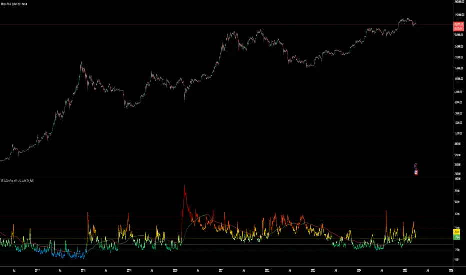
VIX bottom/top with color scale [Ox_kali]📊 Introduction
━━━━━━━━━━━━━━━━━━━━━━━━━━━━━━━━━━━━━━━━━━━
The “VIX Bottom/Top with Color Scale” script is designed to provide an intuitive, color-coded visualization of the VIX (Volatility Index), helping traders interpret market sentiment and volatility extremes in real time.
It segments the VIX into clear threshold zones, each associated with a specific market condition—ranging from fear to calm—using a dynamic color-coded system.
This script offers significant value for the following reasons:
Intuitive Risk Interpretation: Color-coded zones make it easy to interpret market sentiment at a glance.
Dynamic Trend Detection: A 200-period SMA of the VIX is plotted and dynamically colored based on trend direction.
Customization and Flexibility: All colors are editable in the parameters panel, grouped under “## Color parameters ##”.
Visual Clarity: Key thresholds are marked with horizontal lines for quick reference.
Practical Trading Tool: Helps identify high-risk and low-risk environments based on volatility levels.
🔍 Key Indicators
━━━━━━━━━━━━━━━━━━━━━━━━━━━━━━━━━━━━━━━━━━━
VIX (CBOE Volatility Index) : Measures market volatility and investor fear.
SMA 200 : Long-term trendline of the VIX, with color-coded direction (green = uptrend, red = downtrend).
Color-coded VIX Levels:
🔴 33+ → Something bad just happened
🟠 23–33 → Something bad is happening
🟡 17–23 → Something bad might happen
🟢 14–17 → Nothing bad is happening
✅ 12–14 → Nothing bad will ever happen
🔵 <12 → Something bad is going to happen
🧠 Originality and Purpose
━━━━━━━━━━━━━━━━━━━━━━━━━━━━━━━━━━━━━━━━━━━
Unlike traditional VIX indicators that only plot a line, this script enhances interpretation through visual segmentation and dynamic trend tracking.
It serves as a risk-awareness tool that transforms the VIX into a simple, emotional market map.
This is the first version of the script, and future updates may include alerts, background fills, and more advanced features.
⚙️ How It Works
━━━━━━━━━━━━━━━━━━━━━━━━━━━━━━━━━━━━━━━━━━━
The script maps the current VIX value to a range and applies the corresponding color.
It calculates a SMA 200 and colors it green or red depending on its slope.
It displays horizontal dotted lines at key thresholds (12, 14, 17, 23, 33).
All colors are configurable via input parameters under the group: "## Color parameters ##".
🧭 Indicator Visualization and Interpretation
━━━━━━━━━━━━━━━━━━━━━━━━━━━━━━━━━━━━━━━━━━━
The VIX line changes color based on market condition zones.
The SMA line shows long-term direction with dynamic color.
Horizontal threshold lines visually mark the transitions between volatility zones.
Ideal for quickly identifying periods of fear, caution, or stability.
🛠️ Script Parameters
━━━━━━━━━━━━━━━━━━━━━━━━━━━━━━━━━━━━━━━━━━━
Grouped under “## Color parameters ##”, the following elements are customizable:
🎨 VIX Zone Colors:
33+ → Red
23–33 → Orange
17–23 → Yellow
14–17 → Light Green
12–14 → Dark Green
<12 → Blue
📈 SMA Colors:
Uptrend → Green
Downtrend → Red
These settings allow users to match the script’s visuals to their preferred chart style or theme.
✅ Conclusion
━━━━━━━━━━━━━━━━━━━━━━━━━━━━━━━━━━━━━━━━━━━
The “VIX Bottom/Top with Color Scale” is a clean, powerful script designed to simplify how traders view volatility.
By combining long-term trend data with real-time color-coded sentiment analysis, this script becomes a go-to reference for managing risk, timing trades, or simply staying in tune with market mood.
🧪 Notes
━━━━━━━━━━━━━━━━━━━━━━━━━━━━━━━━━━━━━━━━━━━
This is version 1 of the script. More features such as alert conditions, background fill, and dashboard elements may be added soon. Feedback is welcome!
💡 Color code concept inspired by the original VIX interpretation chart by @nsquaredvalue on Twitter. Big thanks for the visual clarity! 💡
⚠️ Disclaimer
━━━━━━━━━━━━━━━━━━━━━━━━━━━━━━━━━━━━━━━━━━━
This script is a visual tool designed to assist in market analysis. It does not guarantee future performance and should be used in conjunction with proper risk management. Past performance is not indicative of future results.
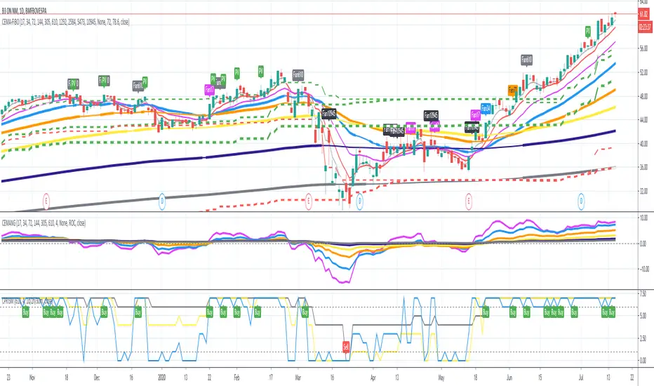
Super EMA PrismThis script implements the Binary Trade Logic (BTL) algorithm to calculate two distinct scores that range from 0 to 7. One score is calculated assigning a power of 2 weight to the positive sign of 3 Phi^3 distant Moving Average (MA) slopes. The other score is calculated assigning a power of 2 weight to the sign of the difference between the price and the value of 3 Phi^3 distant Moving Average (MA).
For the first score, hereafter called as the angle score (AS), the largest MA slope positive sign receives weight 4, the middle length MA slope positive sign receives weight 2 and the shortest MA slope positive sign receives weight 1. The positive sign of an MA is defined as 1 if the slope of the MA is positive and 0, otherwise. Therefore, for MAs 305, 72 and 17, if slope(MA305) > 0, slope(MA72) < 0 and slope(MA17) > 0, then score will be 4*1 + 2*0 + 1*1 = 5. Up to my knowledge, this score was first proposed by Bo Williams and named by him as Prisma.
For the second score, hereafter called as the value score (VS), if the price > largest MA, it receives weight 4. If the price > the middle length MA, it receives weight 2 and if the price > the the shortest MA, it receives weight 1. Therefore, for MAs 305, 72 and 17, if price < MA305, price > MA72 and price > MA17, then score will be 4*0 + 2*1 + 1*1 = 3. Up to my knowledge, this score was first proposed by Bo Williams and named by him as Prisma.
Both AS and VS are calculated for Phi^3 lengths (610, 144, 34) and for Phi^3/2 lengths (305, 72, 17). The scores of the same kind calculated for each set of length are combined multiplying the Phi^3 length score by 10 and adding with with the Phi^3/2 score, therefore providing a 2 digit score ranging from 0 to 77. For instance, if we have AS(610, 144, 34) = 7 and AS(305, 72, 17) = 5, we have AS=75. At the same time, if we have VS(610, 144, 34) = 6 and VS(305, 72, 17) = 4, we have VS=64.
VS score is plotted by default in black, but it can be on white for dark themes. AS is plotted with the color of the longest MA used.
Chart background is colored according to the range of values for AS and VS, checked in the following order:
if AS >= 13 and VS <= 13 then back color = red
if AS >= 13 or VS <= 13 then back color = orange
if AS >= 64 and VS >= 64 then back color = green
if AS >= 64 or VS >= 64 then back color = blue
otherwise back color = none (white o black)

Optimized Future Time Cycles V2Time Cycle-Based Indicator Overview
This script utilizes Time Cycles to visually display the periodic fluctuations of the past and future, helping to predict key market turning points and trend shifts.
The indicator is fully customizable and marks periodic vertical lines and labels on the chart based on a specified reference date.
1. Key Features
Time Cycle Settings
Displays various user-defined time cycles (e.g., 9 days, 17 days, 26 days) visually on the chart.
Each cycle is distinguished by unique colors and labels for clear identification.
Allows users to set a reference date, from which past and future cycles are calculated.
Past and Future Cycle Visualization
Future Cycles:
Predicts potential points of market fluctuations or trend changes in the future.
Vertical lines represent future turning points based on the defined time cycles.
Past Cycles:
Displays how cyclical patterns manifested in historical market data.
Helps identify recurring patterns and similar historical market conditions.
Customizable Visuals
Adjust line styles (solid, dashed, etc.) and label spacing for a cleaner chart, even with multiple cycles displayed.
Separately toggle the visibility of past and future cycles for a more tailored analysis experience.
2. How to Use and Interpret the Indicator
Setting the Reference Date
The reference date is crucial for this indicator and works best when set to significant market events or turning points.
Both past and future cycles are calculated based on the reference date, and overlapping cycles may indicate periods of high volatility or strong trend shifts.
Cycle Analysis
Interpretation by Cycle Duration:
Short-term Cycles (9, 17 days): Useful for predicting quick market fluctuations.
Mid- to Long-term Cycles (26, 52, 200 days): Ideal for identifying major trend changes.
Overlapping Cycles:
When multiple cycles converge, significant turning points or strong market movements are likely.
Importance of Past Cycles
Past cycles are invaluable for identifying repetitive patterns in the market.
For example, analyzing strong turning points from past cycles can help anticipate similar scenarios in the future.
3. Tips for Using the Indicator
Optimize Line Styles:
When displaying both past and future cycles, charts may become cluttered. Adjusting line styles or colors can help maintain visual clarity.
Short-term vs. Long-term Cycles:
Short-term Cycles: Best suited for strategies like scalping or day trading.
Long-term Cycles: Useful for capturing major trend shifts or identifying macroeconomic changes.
Recommended Combination with Other Indicators:
Combine the Time Cycle indicator with moving averages, wave indicators, RSI, or Bollinger Bands for better results.
The time cycle identifies the timing of turning points, while tools like moving averages or RSI provide insights into trend direction during these critical moments.
4. Conclusion
This Time Cycle indicator visualizes past and future periodic fluctuations, enabling effective predictions of market trends and turning points.
The reference date and overlapping cycles are essential for pinpointing critical turning points.
The newly added past cycle visualization feature enhances the ability to recognize recurring patterns and leverage historical data for more accurate predictions.
시간 주기(Time Cycle) 기반 지표 소개
이 스크립트는 **시간 주기(Time Cycle)**를 활용해 과거와 미래의 주기적 변동을 시각적으로 보여주어, 시장의 추세 변화 시점과 변곡점을 예측하는 데 도움을 줍니다.
지표는 사용자 정의가 가능하며, 설정된 기준 날짜를 기반으로 주기적인 수직선과 레이블을 차트에 표시합니다.
1. 주요 기능
시간 주기 설정
사용자가 설정한 다양한 시간 주기(예: 9일, 17일, 26일 등)를 시각적으로 표시.
각 주기는 고유한 색상과 레이블로 구분되어 명확하게 차트에 나타납니다.
**기준 날짜(reference date)**를 설정하여, 해당 날짜를 기준으로 과거와 미래의 주기를 계산합니다.
미래와 과거 주기 표시
미래 주기:
미래의 시장 변동 시점이나 추세 변화 가능성이 높은 지점을 예측할 수 있습니다.
설정된 시간 주기에 따라 미래 변곡점을 차트에 수직선으로 나타냅니다.
과거 주기:
과거 시장에서 주기적 변동이 어떻게 나타났는지 확인 가능합니다.
이를 통해 반복되는 패턴이나 과거와 유사한 시장 상황을 파악할 수 있습니다.
시각적 사용자 설정
수직선 스타일(실선, 점선 등)과 레이블 간격을 조정하여, 복잡한 차트에서도 깔끔하게 정보를 확인할 수 있습니다.
과거와 미래의 주기 표시를 개별적으로 조정 가능하여 사용자 맞춤형 분석이 가능합니다.
2. 지표 사용 및 해석 방법
기준 날짜 설정
**기준 날짜(reference date)**는 시장에서 중요한 변동이 있었던 날을 기준으로 설정하는 것이 가장 효과적입니다.
기준 날짜를 기반으로 과거와 미래 주기가 계산되며, 주기가 겹치는 시점에서 강한 변동성이 나타날 가능성이 높습니다.
주기 분석
주기별 해석:
단기 주기 (9일, 17일): 빠른 변동성을 예측.
중·장기 주기 (26일, 52일, 200일): 큰 추세 변화를 예측.
주기가 겹치는 시점은 중요한 변곡점이 될 가능성이 크며, 추세 전환의 신호로 볼 수 있습니다.
과거 주기의 중요성
과거 주기는 시장의 반복 패턴을 찾는 데 유용합니다.
예를 들어, 과거 주기에서 강한 변곡점이 나타났던 시점을 분석하면, 미래에도 유사한 상황이 발생할 가능성을 예측할 수 있습니다.
3. 지표 활용 팁
수직선 스타일 최적화:
과거와 미래 주기를 모두 표시하면 차트가 복잡해질 수 있으므로, 선 스타일이나 색상을 조정하여 시각적으로 덜 혼란스럽게 설정하세요.
단기 vs. 장기 주기:
단기 주기는 스캘핑과 같은 빠른 매매 전략에 유용하며,
장기 주기는 대세 추세 변화를 포착하는 데 유리합니다.
결합 사용 추천:
시간 주기(Time Cycle) 지표는 이평선 파동 지표 또는 RSI, 볼린저 밴드와 함께 사용하면 더욱 효과적입니다.
시간 주기는 변곡점의 시점을 알려주고, 이평선 파동이나 RSI는 그 시점에서의 추세 방향성을 보완해 줍니다.
4. 결론
이 시간 주기(Time Cycle) 지표는 과거와 미래의 주기적 변동을 시각화하여, 시장의 추세 변화와 변곡점을 효과적으로 예측할 수 있습니다.
특히, 기준 날짜 설정과 주기적 겹침은 중요한 변곡점을 파악하는 핵심입니다.
새롭게 추가된 과거 주기 표시 기능은 반복 패턴을 확인하고 과거 데이터를 바탕으로 더 정교한 예측을 가능하게 합니다.

Cycles 90mThe cycles are separated by vertical lines. The first cycle (Q1) is marked with a red line because it is a manipulative cycle where you should not open positions. Other cycles are green (Q2, Q3, Q4).
You can add the time of the current candle, its size and position on the chart in the settings
The time is highlighted in red in the timeframes 9:30-9:40, 10:00-10:10, 11:00-11:30, 15:30-15:40, 16:00-16:10, 17:00-17:10, 17:30-17:40, as price movements are most often expected during these timeframes.
The cycle lines automatically disappear if you open a timeframe above M15

Custom EMA PrismThis script implements the Binary Logic Trading (BLT) algorithm to calculate a score from 0 to 7. This score is calculated assigning a power of 2 weight to the positive sign of 3 Phi^3 distant EMAs' slopes. The largest EMA slope positive sign receives weight 4, the middle length EMA slope positive sign receives weight 2 and the shortest EMA slope positive sign receives weight 1. The positive sign of an EMA is defined as 1 if the slope of the EMA is positive and 0, otherwise. Therefore, for EMAs 305, 72 and 17, if slope(EMA305) > 0, slope(EMA72) < 0 and slope(EMA17) > 0, then score will be 4*1 + 2*0 + 1*1 = 5. Up to my knowledge, this score was first proposed by Bo Williams and named by him as Prisma.
Due too sampling issues, this script ONLY WORKS with graphic time of 1d. I would like to thanks to MrBitmanBob for showing me how to get quotations from a graphic time distinct from the current one.
This script also gets sampling data from graphic times 2h and 30m to calculate their score. As, even for smaller graphic times, price data is sampled at the current time frequency, the EMA lengths for those smaller graphic times needed to be proportionally decreased, meaning that when calculating the score for 1d with lengths 305, 72 and 17, the score for 2h must be calculated with lengths 72, 17 and 4, and the score for 30m must be calculated with lengths 17, 4 an 1. I understand that some precision may be lost but it is the best that is possible.
There is an optional setting for Crypto Currencies that instead of calculating the score for 1d, 2h and 30m, it calculates the score for 1d, 4h and 60m. This is due to the fact that Crypto Currencies are traded 24x7. Despite of this setting, the labels at the Style tab of the settings window remains 2h and 30m, because they must be constants.
This script with the corresponding EMAs chart and the EMAs Angle chart provides a broader view of the trading scenario.
Markov Chain [3D] | FractalystWhat exactly is a Markov Chain?
This indicator uses a Markov Chain model to analyze, quantify, and visualize the transitions between market regimes (Bull, Bear, Neutral) on your chart. It dynamically detects these regimes in real-time, calculates transition probabilities, and displays them as animated 3D spheres and arrows, giving traders intuitive insight into current and future market conditions.
How does a Markov Chain work, and how should I read this spheres-and-arrows diagram?
Think of three weather modes: Sunny, Rainy, Cloudy.
Each sphere is one mode. The loop on a sphere means “stay the same next step” (e.g., Sunny again tomorrow).
The arrows leaving a sphere show where things usually go next if they change (e.g., Sunny moving to Cloudy).
Some paths matter more than others. A more prominent loop means the current mode tends to persist. A more prominent outgoing arrow means a change to that destination is the usual next step.
Direction isn’t symmetric: moving Sunny→Cloudy can behave differently than Cloudy→Sunny.
Now relabel the spheres to markets: Bull, Bear, Neutral.
Spheres: market regimes (uptrend, downtrend, range).
Self‑loop: tendency for the current regime to continue on the next bar.
Arrows: the most common next regime if a switch happens.
How to read: Start at the sphere that matches current bar state. If the loop stands out, expect continuation. If one outgoing path stands out, that switch is the typical next step. Opposite directions can differ (Bear→Neutral doesn’t have to match Neutral→Bear).
What states and transitions are shown?
The three market states visualized are:
Bullish (Bull): Upward or strong-market regime.
Bearish (Bear): Downward or weak-market regime.
Neutral: Sideways or range-bound regime.
Bidirectional animated arrows and probability labels show how likely the market is to move from one regime to another (e.g., Bull → Bear or Neutral → Bull).
How does the regime detection system work?
You can use either built-in price returns (based on adaptive Z-score normalization) or supply three custom indicators (such as volume, oscillators, etc.).
Values are statistically normalized (Z-scored) over a configurable lookback period.
The normalized outputs are classified into Bull, Bear, or Neutral zones.
If using three indicators, their regime signals are averaged and smoothed for robustness.
How are transition probabilities calculated?
On every confirmed bar, the algorithm tracks the sequence of detected market states, then builds a rolling window of transitions.
The code maintains a transition count matrix for all regime pairs (e.g., Bull → Bear).
Transition probabilities are extracted for each possible state change using Laplace smoothing for numerical stability, and frequently updated in real-time.
What is unique about the visualization?
3D animated spheres represent each regime and change visually when active.
Animated, bidirectional arrows reveal transition probabilities and allow you to see both dominant and less likely regime flows.
Particles (moving dots) animate along the arrows, enhancing the perception of regime flow direction and speed.
All elements dynamically update with each new price bar, providing a live market map in an intuitive, engaging format.
Can I use custom indicators for regime classification?
Yes! Enable the "Custom Indicators" switch and select any three chart series as inputs. These will be normalized and combined (each with equal weight), broadening the regime classification beyond just price-based movement.
What does the “Lookback Period” control?
Lookback Period (default: 100) sets how much historical data builds the probability matrix. Shorter periods adapt faster to regime changes but may be noisier. Longer periods are more stable but slower to adapt.
How is this different from a Hidden Markov Model (HMM)?
It sets the window for both regime detection and probability calculations. Lower values make the system more reactive, but potentially noisier. Higher values smooth estimates and make the system more robust.
How is this Markov Chain different from a Hidden Markov Model (HMM)?
Markov Chain (as here): All market regimes (Bull, Bear, Neutral) are directly observable on the chart. The transition matrix is built from actual detected regimes, keeping the model simple and interpretable.
Hidden Markov Model: The actual regimes are unobservable ("hidden") and must be inferred from market output or indicator "emissions" using statistical learning algorithms. HMMs are more complex, can capture more subtle structure, but are harder to visualize and require additional machine learning steps for training.
A standard Markov Chain models transitions between observable states using a simple transition matrix, while a Hidden Markov Model assumes the true states are hidden (latent) and must be inferred from observable “emissions” like price or volume data. In practical terms, a Markov Chain is transparent and easier to implement and interpret; an HMM is more expressive but requires statistical inference to estimate hidden states from data.
Markov Chain: states are observable; you directly count or estimate transition probabilities between visible states. This makes it simpler, faster, and easier to validate and tune.
HMM: states are hidden; you only observe emissions generated by those latent states. Learning involves machine learning/statistical algorithms (commonly Baum–Welch/EM for training and Viterbi for decoding) to infer both the transition dynamics and the most likely hidden state sequence from data.
How does the indicator avoid “repainting” or look-ahead bias?
All regime changes and matrix updates happen only on confirmed (closed) bars, so no future data is leaked, ensuring reliable real-time operation.
Are there practical tuning tips?
Tune the Lookback Period for your asset/timeframe: shorter for fast markets, longer for stability.
Use custom indicators if your asset has unique regime drivers.
Watch for rapid changes in transition probabilities as early warning of a possible regime shift.
Who is this indicator for?
Quants and quantitative researchers exploring probabilistic market modeling, especially those interested in regime-switching dynamics and Markov models.
Programmers and system developers who need a probabilistic regime filter for systematic and algorithmic backtesting:
The Markov Chain indicator is ideally suited for programmatic integration via its bias output (1 = Bull, 0 = Neutral, -1 = Bear).
Although the visualization is engaging, the core output is designed for automated, rules-based workflows—not for discretionary/manual trading decisions.
Developers can connect the indicator’s output directly to their Pine Script logic (using input.source()), allowing rapid and robust backtesting of regime-based strategies.
It acts as a plug-and-play regime filter: simply plug the bias output into your entry/exit logic, and you have a scientifically robust, probabilistically-derived signal for filtering, timing, position sizing, or risk regimes.
The MC's output is intentionally "trinary" (1/0/-1), focusing on clear regime states for unambiguous decision-making in code. If you require nuanced, multi-probability or soft-label state vectors, consider expanding the indicator or stacking it with a probability-weighted logic layer in your scripting.
Because it avoids subjectivity, this approach is optimal for systematic quants, algo developers building backtested, repeatable strategies based on probabilistic regime analysis.
What's the mathematical foundation behind this?
The mathematical foundation behind this Markov Chain indicator—and probabilistic regime detection in finance—draws from two principal models: the (standard) Markov Chain and the Hidden Markov Model (HMM).
How to use this indicator programmatically?
The Markov Chain indicator automatically exports a bias value (+1 for Bullish, -1 for Bearish, 0 for Neutral) as a plot visible in the Data Window. This allows you to integrate its regime signal into your own scripts and strategies for backtesting, automation, or live trading.
Step-by-Step Integration with Pine Script (input.source)
Add the Markov Chain indicator to your chart.
This must be done first, since your custom script will "pull" the bias signal from the indicator's plot.
In your strategy, create an input using input.source()
Example:
//@version=5
strategy("MC Bias Strategy Example")
mcBias = input.source(close, "MC Bias Source")
After saving, go to your script’s settings. For the “MC Bias Source” input, select the plot/output of the Markov Chain indicator (typically its bias plot).
Use the bias in your trading logic
Example (long only on Bull, flat otherwise):
if mcBias == 1
strategy.entry("Long", strategy.long)
else
strategy.close("Long")
For more advanced workflows, combine mcBias with additional filters or trailing stops.
How does this work behind-the-scenes?
TradingView’s input.source() lets you use any plot from another indicator as a real-time, “live” data feed in your own script (source).
The selected bias signal is available to your Pine code as a variable, enabling logical decisions based on regime (trend-following, mean-reversion, etc.).
This enables powerful strategy modularity : decouple regime detection from entry/exit logic, allowing fast experimentation without rewriting core signal code.
Integrating 45+ Indicators with Your Markov Chain — How & Why
The Enhanced Custom Indicators Export script exports a massive suite of over 45 technical indicators—ranging from classic momentum (RSI, MACD, Stochastic, etc.) to trend, volume, volatility, and oscillator tools—all pre-calculated, centered/scaled, and available as plots.
// Enhanced Custom Indicators Export - 45 Technical Indicators
// Comprehensive technical analysis suite for advanced market regime detection
//@version=6
indicator('Enhanced Custom Indicators Export | Fractalyst', shorttitle='Enhanced CI Export', overlay=false, scale=scale.right, max_labels_count=500, max_lines_count=500)
// |----- Input Parameters -----| //
momentum_group = "Momentum Indicators"
trend_group = "Trend Indicators"
volume_group = "Volume Indicators"
volatility_group = "Volatility Indicators"
oscillator_group = "Oscillator Indicators"
display_group = "Display Settings"
// Common lengths
length_14 = input.int(14, "Standard Length (14)", minval=1, maxval=100, group=momentum_group)
length_20 = input.int(20, "Medium Length (20)", minval=1, maxval=200, group=trend_group)
length_50 = input.int(50, "Long Length (50)", minval=1, maxval=200, group=trend_group)
// Display options
show_table = input.bool(true, "Show Values Table", group=display_group)
table_size = input.string("Small", "Table Size", options= , group=display_group)
// |----- MOMENTUM INDICATORS (15 indicators) -----| //
// 1. RSI (Relative Strength Index)
rsi_14 = ta.rsi(close, length_14)
rsi_centered = rsi_14 - 50
// 2. Stochastic Oscillator
stoch_k = ta.stoch(close, high, low, length_14)
stoch_d = ta.sma(stoch_k, 3)
stoch_centered = stoch_k - 50
// 3. Williams %R
williams_r = ta.stoch(close, high, low, length_14) - 100
// 4. MACD (Moving Average Convergence Divergence)
= ta.macd(close, 12, 26, 9)
// 5. Momentum (Rate of Change)
momentum = ta.mom(close, length_14)
momentum_pct = (momentum / close ) * 100
// 6. Rate of Change (ROC)
roc = ta.roc(close, length_14)
// 7. Commodity Channel Index (CCI)
cci = ta.cci(close, length_20)
// 8. Money Flow Index (MFI)
mfi = ta.mfi(close, length_14)
mfi_centered = mfi - 50
// 9. Awesome Oscillator (AO)
ao = ta.sma(hl2, 5) - ta.sma(hl2, 34)
// 10. Accelerator Oscillator (AC)
ac = ao - ta.sma(ao, 5)
// 11. Chande Momentum Oscillator (CMO)
cmo = ta.cmo(close, length_14)
// 12. Detrended Price Oscillator (DPO)
dpo = close - ta.sma(close, length_20)
// 13. Price Oscillator (PPO)
ppo = ta.sma(close, 12) - ta.sma(close, 26)
ppo_pct = (ppo / ta.sma(close, 26)) * 100
// 14. TRIX
trix_ema1 = ta.ema(close, length_14)
trix_ema2 = ta.ema(trix_ema1, length_14)
trix_ema3 = ta.ema(trix_ema2, length_14)
trix = ta.roc(trix_ema3, 1) * 10000
// 15. Klinger Oscillator
klinger = ta.ema(volume * (high + low + close) / 3, 34) - ta.ema(volume * (high + low + close) / 3, 55)
// 16. Fisher Transform
fisher_hl2 = 0.5 * (hl2 - ta.lowest(hl2, 10)) / (ta.highest(hl2, 10) - ta.lowest(hl2, 10)) - 0.25
fisher = 0.5 * math.log((1 + fisher_hl2) / (1 - fisher_hl2))
// 17. Stochastic RSI
stoch_rsi = ta.stoch(rsi_14, rsi_14, rsi_14, length_14)
stoch_rsi_centered = stoch_rsi - 50
// 18. Relative Vigor Index (RVI)
rvi_num = ta.swma(close - open)
rvi_den = ta.swma(high - low)
rvi = rvi_den != 0 ? rvi_num / rvi_den : 0
// 19. Balance of Power (BOP)
bop = (close - open) / (high - low)
// |----- TREND INDICATORS (10 indicators) -----| //
// 20. Simple Moving Average Momentum
sma_20 = ta.sma(close, length_20)
sma_momentum = ((close - sma_20) / sma_20) * 100
// 21. Exponential Moving Average Momentum
ema_20 = ta.ema(close, length_20)
ema_momentum = ((close - ema_20) / ema_20) * 100
// 22. Parabolic SAR
sar = ta.sar(0.02, 0.02, 0.2)
sar_trend = close > sar ? 1 : -1
// 23. Linear Regression Slope
lr_slope = ta.linreg(close, length_20, 0) - ta.linreg(close, length_20, 1)
// 24. Moving Average Convergence (MAC)
mac = ta.sma(close, 10) - ta.sma(close, 30)
// 25. Trend Intensity Index (TII)
tii_sum = 0.0
for i = 1 to length_20
tii_sum += close > close ? 1 : 0
tii = (tii_sum / length_20) * 100
// 26. Ichimoku Cloud Components
ichimoku_tenkan = (ta.highest(high, 9) + ta.lowest(low, 9)) / 2
ichimoku_kijun = (ta.highest(high, 26) + ta.lowest(low, 26)) / 2
ichimoku_signal = ichimoku_tenkan > ichimoku_kijun ? 1 : -1
// 27. MESA Adaptive Moving Average (MAMA)
mama_alpha = 2.0 / (length_20 + 1)
mama = ta.ema(close, length_20)
mama_momentum = ((close - mama) / mama) * 100
// 28. Zero Lag Exponential Moving Average (ZLEMA)
zlema_lag = math.round((length_20 - 1) / 2)
zlema_data = close + (close - close )
zlema = ta.ema(zlema_data, length_20)
zlema_momentum = ((close - zlema) / zlema) * 100
// |----- VOLUME INDICATORS (6 indicators) -----| //
// 29. On-Balance Volume (OBV)
obv = ta.obv
// 30. Volume Rate of Change (VROC)
vroc = ta.roc(volume, length_14)
// 31. Price Volume Trend (PVT)
pvt = ta.pvt
// 32. Negative Volume Index (NVI)
nvi = 0.0
nvi := volume < volume ? nvi + ((close - close ) / close ) * nvi : nvi
// 33. Positive Volume Index (PVI)
pvi = 0.0
pvi := volume > volume ? pvi + ((close - close ) / close ) * pvi : pvi
// 34. Volume Oscillator
vol_osc = ta.sma(volume, 5) - ta.sma(volume, 10)
// 35. Ease of Movement (EOM)
eom_distance = high - low
eom_box_height = volume / 1000000
eom = eom_box_height != 0 ? eom_distance / eom_box_height : 0
eom_sma = ta.sma(eom, length_14)
// 36. Force Index
force_index = volume * (close - close )
force_index_sma = ta.sma(force_index, length_14)
// |----- VOLATILITY INDICATORS (10 indicators) -----| //
// 37. Average True Range (ATR)
atr = ta.atr(length_14)
atr_pct = (atr / close) * 100
// 38. Bollinger Bands Position
bb_basis = ta.sma(close, length_20)
bb_dev = 2.0 * ta.stdev(close, length_20)
bb_upper = bb_basis + bb_dev
bb_lower = bb_basis - bb_dev
bb_position = bb_dev != 0 ? (close - bb_basis) / bb_dev : 0
bb_width = bb_dev != 0 ? (bb_upper - bb_lower) / bb_basis * 100 : 0
// 39. Keltner Channels Position
kc_basis = ta.ema(close, length_20)
kc_range = ta.ema(ta.tr, length_20)
kc_upper = kc_basis + (2.0 * kc_range)
kc_lower = kc_basis - (2.0 * kc_range)
kc_position = kc_range != 0 ? (close - kc_basis) / kc_range : 0
// 40. Donchian Channels Position
dc_upper = ta.highest(high, length_20)
dc_lower = ta.lowest(low, length_20)
dc_basis = (dc_upper + dc_lower) / 2
dc_position = (dc_upper - dc_lower) != 0 ? (close - dc_basis) / (dc_upper - dc_lower) : 0
// 41. Standard Deviation
std_dev = ta.stdev(close, length_20)
std_dev_pct = (std_dev / close) * 100
// 42. Relative Volatility Index (RVI)
rvi_up = ta.stdev(close > close ? close : 0, length_14)
rvi_down = ta.stdev(close < close ? close : 0, length_14)
rvi_total = rvi_up + rvi_down
rvi_volatility = rvi_total != 0 ? (rvi_up / rvi_total) * 100 : 50
// 43. Historical Volatility
hv_returns = math.log(close / close )
hv = ta.stdev(hv_returns, length_20) * math.sqrt(252) * 100
// 44. Garman-Klass Volatility
gk_vol = math.log(high/low) * math.log(high/low) - (2*math.log(2)-1) * math.log(close/open) * math.log(close/open)
gk_volatility = math.sqrt(ta.sma(gk_vol, length_20)) * 100
// 45. Parkinson Volatility
park_vol = math.log(high/low) * math.log(high/low)
parkinson = math.sqrt(ta.sma(park_vol, length_20) / (4 * math.log(2))) * 100
// 46. Rogers-Satchell Volatility
rs_vol = math.log(high/close) * math.log(high/open) + math.log(low/close) * math.log(low/open)
rogers_satchell = math.sqrt(ta.sma(rs_vol, length_20)) * 100
// |----- OSCILLATOR INDICATORS (5 indicators) -----| //
// 47. Elder Ray Index
elder_bull = high - ta.ema(close, 13)
elder_bear = low - ta.ema(close, 13)
elder_power = elder_bull + elder_bear
// 48. Schaff Trend Cycle (STC)
stc_macd = ta.ema(close, 23) - ta.ema(close, 50)
stc_k = ta.stoch(stc_macd, stc_macd, stc_macd, 10)
stc_d = ta.ema(stc_k, 3)
stc = ta.stoch(stc_d, stc_d, stc_d, 10)
// 49. Coppock Curve
coppock_roc1 = ta.roc(close, 14)
coppock_roc2 = ta.roc(close, 11)
coppock = ta.wma(coppock_roc1 + coppock_roc2, 10)
// 50. Know Sure Thing (KST)
kst_roc1 = ta.roc(close, 10)
kst_roc2 = ta.roc(close, 15)
kst_roc3 = ta.roc(close, 20)
kst_roc4 = ta.roc(close, 30)
kst = ta.sma(kst_roc1, 10) + 2*ta.sma(kst_roc2, 10) + 3*ta.sma(kst_roc3, 10) + 4*ta.sma(kst_roc4, 15)
// 51. Percentage Price Oscillator (PPO)
ppo_line = ((ta.ema(close, 12) - ta.ema(close, 26)) / ta.ema(close, 26)) * 100
ppo_signal = ta.ema(ppo_line, 9)
ppo_histogram = ppo_line - ppo_signal
// |----- PLOT MAIN INDICATORS -----| //
// Plot key momentum indicators
plot(rsi_centered, title="01_RSI_Centered", color=color.purple, linewidth=1)
plot(stoch_centered, title="02_Stoch_Centered", color=color.blue, linewidth=1)
plot(williams_r, title="03_Williams_R", color=color.red, linewidth=1)
plot(macd_histogram, title="04_MACD_Histogram", color=color.orange, linewidth=1)
plot(cci, title="05_CCI", color=color.green, linewidth=1)
// Plot trend indicators
plot(sma_momentum, title="06_SMA_Momentum", color=color.navy, linewidth=1)
plot(ema_momentum, title="07_EMA_Momentum", color=color.maroon, linewidth=1)
plot(sar_trend, title="08_SAR_Trend", color=color.teal, linewidth=1)
plot(lr_slope, title="09_LR_Slope", color=color.lime, linewidth=1)
plot(mac, title="10_MAC", color=color.fuchsia, linewidth=1)
// Plot volatility indicators
plot(atr_pct, title="11_ATR_Pct", color=color.yellow, linewidth=1)
plot(bb_position, title="12_BB_Position", color=color.aqua, linewidth=1)
plot(kc_position, title="13_KC_Position", color=color.olive, linewidth=1)
plot(std_dev_pct, title="14_StdDev_Pct", color=color.silver, linewidth=1)
plot(bb_width, title="15_BB_Width", color=color.gray, linewidth=1)
// Plot volume indicators
plot(vroc, title="16_VROC", color=color.blue, linewidth=1)
plot(eom_sma, title="17_EOM", color=color.red, linewidth=1)
plot(vol_osc, title="18_Vol_Osc", color=color.green, linewidth=1)
plot(force_index_sma, title="19_Force_Index", color=color.orange, linewidth=1)
plot(obv, title="20_OBV", color=color.purple, linewidth=1)
// Plot additional oscillators
plot(ao, title="21_Awesome_Osc", color=color.navy, linewidth=1)
plot(cmo, title="22_CMO", color=color.maroon, linewidth=1)
plot(dpo, title="23_DPO", color=color.teal, linewidth=1)
plot(trix, title="24_TRIX", color=color.lime, linewidth=1)
plot(fisher, title="25_Fisher", color=color.fuchsia, linewidth=1)
// Plot more momentum indicators
plot(mfi_centered, title="26_MFI_Centered", color=color.yellow, linewidth=1)
plot(ac, title="27_AC", color=color.aqua, linewidth=1)
plot(ppo_pct, title="28_PPO_Pct", color=color.olive, linewidth=1)
plot(stoch_rsi_centered, title="29_StochRSI_Centered", color=color.silver, linewidth=1)
plot(klinger, title="30_Klinger", color=color.gray, linewidth=1)
// Plot trend continuation
plot(tii, title="31_TII", color=color.blue, linewidth=1)
plot(ichimoku_signal, title="32_Ichimoku_Signal", color=color.red, linewidth=1)
plot(mama_momentum, title="33_MAMA_Momentum", color=color.green, linewidth=1)
plot(zlema_momentum, title="34_ZLEMA_Momentum", color=color.orange, linewidth=1)
plot(bop, title="35_BOP", color=color.purple, linewidth=1)
// Plot volume continuation
plot(nvi, title="36_NVI", color=color.navy, linewidth=1)
plot(pvi, title="37_PVI", color=color.maroon, linewidth=1)
plot(momentum_pct, title="38_Momentum_Pct", color=color.teal, linewidth=1)
plot(roc, title="39_ROC", color=color.lime, linewidth=1)
plot(rvi, title="40_RVI", color=color.fuchsia, linewidth=1)
// Plot volatility continuation
plot(dc_position, title="41_DC_Position", color=color.yellow, linewidth=1)
plot(rvi_volatility, title="42_RVI_Volatility", color=color.aqua, linewidth=1)
plot(hv, title="43_Historical_Vol", color=color.olive, linewidth=1)
plot(gk_volatility, title="44_GK_Volatility", color=color.silver, linewidth=1)
plot(parkinson, title="45_Parkinson_Vol", color=color.gray, linewidth=1)
// Plot final oscillators
plot(rogers_satchell, title="46_RS_Volatility", color=color.blue, linewidth=1)
plot(elder_power, title="47_Elder_Power", color=color.red, linewidth=1)
plot(stc, title="48_STC", color=color.green, linewidth=1)
plot(coppock, title="49_Coppock", color=color.orange, linewidth=1)
plot(kst, title="50_KST", color=color.purple, linewidth=1)
// Plot final indicators
plot(ppo_histogram, title="51_PPO_Histogram", color=color.navy, linewidth=1)
plot(pvt, title="52_PVT", color=color.maroon, linewidth=1)
// |----- Reference Lines -----| //
hline(0, "Zero Line", color=color.gray, linestyle=hline.style_dashed, linewidth=1)
hline(50, "Midline", color=color.gray, linestyle=hline.style_dotted, linewidth=1)
hline(-50, "Lower Midline", color=color.gray, linestyle=hline.style_dotted, linewidth=1)
hline(25, "Upper Threshold", color=color.gray, linestyle=hline.style_dotted, linewidth=1)
hline(-25, "Lower Threshold", color=color.gray, linestyle=hline.style_dotted, linewidth=1)
// |----- Enhanced Information Table -----| //
if show_table and barstate.islast
table_position = position.top_right
table_text_size = table_size == "Tiny" ? size.tiny : table_size == "Small" ? size.small : size.normal
var table info_table = table.new(table_position, 3, 18, bgcolor=color.new(color.white, 85), border_width=1, border_color=color.gray)
// Headers
table.cell(info_table, 0, 0, 'Category', text_color=color.black, text_size=table_text_size, bgcolor=color.new(color.blue, 70))
table.cell(info_table, 1, 0, 'Indicator', text_color=color.black, text_size=table_text_size, bgcolor=color.new(color.blue, 70))
table.cell(info_table, 2, 0, 'Value', text_color=color.black, text_size=table_text_size, bgcolor=color.new(color.blue, 70))
// Key Momentum Indicators
table.cell(info_table, 0, 1, 'MOMENTUM', text_color=color.purple, text_size=table_text_size, bgcolor=color.new(color.purple, 90))
table.cell(info_table, 1, 1, 'RSI Centered', text_color=color.purple, text_size=table_text_size)
table.cell(info_table, 2, 1, str.tostring(rsi_centered, '0.00'), text_color=color.purple, text_size=table_text_size)
table.cell(info_table, 0, 2, '', text_color=color.blue, text_size=table_text_size)
table.cell(info_table, 1, 2, 'Stoch Centered', text_color=color.blue, text_size=table_text_size)
table.cell(info_table, 2, 2, str.tostring(stoch_centered, '0.00'), text_color=color.blue, text_size=table_text_size)
table.cell(info_table, 0, 3, '', text_color=color.red, text_size=table_text_size)
table.cell(info_table, 1, 3, 'Williams %R', text_color=color.red, text_size=table_text_size)
table.cell(info_table, 2, 3, str.tostring(williams_r, '0.00'), text_color=color.red, text_size=table_text_size)
table.cell(info_table, 0, 4, '', text_color=color.orange, text_size=table_text_size)
table.cell(info_table, 1, 4, 'MACD Histogram', text_color=color.orange, text_size=table_text_size)
table.cell(info_table, 2, 4, str.tostring(macd_histogram, '0.000'), text_color=color.orange, text_size=table_text_size)
table.cell(info_table, 0, 5, '', text_color=color.green, text_size=table_text_size)
table.cell(info_table, 1, 5, 'CCI', text_color=color.green, text_size=table_text_size)
table.cell(info_table, 2, 5, str.tostring(cci, '0.00'), text_color=color.green, text_size=table_text_size)
// Key Trend Indicators
table.cell(info_table, 0, 6, 'TREND', text_color=color.navy, text_size=table_text_size, bgcolor=color.new(color.navy, 90))
table.cell(info_table, 1, 6, 'SMA Momentum %', text_color=color.navy, text_size=table_text_size)
table.cell(info_table, 2, 6, str.tostring(sma_momentum, '0.00'), text_color=color.navy, text_size=table_text_size)
table.cell(info_table, 0, 7, '', text_color=color.maroon, text_size=table_text_size)
table.cell(info_table, 1, 7, 'EMA Momentum %', text_color=color.maroon, text_size=table_text_size)
table.cell(info_table, 2, 7, str.tostring(ema_momentum, '0.00'), text_color=color.maroon, text_size=table_text_size)
table.cell(info_table, 0, 8, '', text_color=color.teal, text_size=table_text_size)
table.cell(info_table, 1, 8, 'SAR Trend', text_color=color.teal, text_size=table_text_size)
table.cell(info_table, 2, 8, str.tostring(sar_trend, '0'), text_color=color.teal, text_size=table_text_size)
table.cell(info_table, 0, 9, '', text_color=color.lime, text_size=table_text_size)
table.cell(info_table, 1, 9, 'Linear Regression', text_color=color.lime, text_size=table_text_size)
table.cell(info_table, 2, 9, str.tostring(lr_slope, '0.000'), text_color=color.lime, text_size=table_text_size)
// Key Volatility Indicators
table.cell(info_table, 0, 10, 'VOLATILITY', text_color=color.yellow, text_size=table_text_size, bgcolor=color.new(color.yellow, 90))
table.cell(info_table, 1, 10, 'ATR %', text_color=color.yellow, text_size=table_text_size)
table.cell(info_table, 2, 10, str.tostring(atr_pct, '0.00'), text_color=color.yellow, text_size=table_text_size)
table.cell(info_table, 0, 11, '', text_color=color.aqua, text_size=table_text_size)
table.cell(info_table, 1, 11, 'BB Position', text_color=color.aqua, text_size=table_text_size)
table.cell(info_table, 2, 11, str.tostring(bb_position, '0.00'), text_color=color.aqua, text_size=table_text_size)
table.cell(info_table, 0, 12, '', text_color=color.olive, text_size=table_text_size)
table.cell(info_table, 1, 12, 'KC Position', text_color=color.olive, text_size=table_text_size)
table.cell(info_table, 2, 12, str.tostring(kc_position, '0.00'), text_color=color.olive, text_size=table_text_size)
// Key Volume Indicators
table.cell(info_table, 0, 13, 'VOLUME', text_color=color.blue, text_size=table_text_size, bgcolor=color.new(color.blue, 90))
table.cell(info_table, 1, 13, 'Volume ROC', text_color=color.blue, text_size=table_text_size)
table.cell(info_table, 2, 13, str.tostring(vroc, '0.00'), text_color=color.blue, text_size=table_text_size)
table.cell(info_table, 0, 14, '', text_color=color.red, text_size=table_text_size)
table.cell(info_table, 1, 14, 'EOM', text_color=color.red, text_size=table_text_size)
table.cell(info_table, 2, 14, str.tostring(eom_sma, '0.000'), text_color=color.red, text_size=table_text_size)
// Key Oscillators
table.cell(info_table, 0, 15, 'OSCILLATORS', text_color=color.purple, text_size=table_text_size, bgcolor=color.new(color.purple, 90))
table.cell(info_table, 1, 15, 'Awesome Osc', text_color=color.blue, text_size=table_text_size)
table.cell(info_table, 2, 15, str.tostring(ao, '0.000'), text_color=color.blue, text_size=table_text_size)
table.cell(info_table, 0, 16, '', text_color=color.red, text_size=table_text_size)
table.cell(info_table, 1, 16, 'Fisher Transform', text_color=color.red, text_size=table_text_size)
table.cell(info_table, 2, 16, str.tostring(fisher, '0.000'), text_color=color.red, text_size=table_text_size)
// Summary Statistics
table.cell(info_table, 0, 17, 'SUMMARY', text_color=color.black, text_size=table_text_size, bgcolor=color.new(color.gray, 70))
table.cell(info_table, 1, 17, 'Total Indicators: 52', text_color=color.black, text_size=table_text_size)
regime_color = rsi_centered > 10 ? color.green : rsi_centered < -10 ? color.red : color.gray
regime_text = rsi_centered > 10 ? "BULLISH" : rsi_centered < -10 ? "BEARISH" : "NEUTRAL"
table.cell(info_table, 2, 17, regime_text, text_color=regime_color, text_size=table_text_size)
This makes it the perfect “indicator backbone” for quantitative and systematic traders who want to prototype, combine, and test new regime detection models—especially in combination with the Markov Chain indicator.
How to use this script with the Markov Chain for research and backtesting:
Add the Enhanced Indicator Export to your chart.
Every calculated indicator is available as an individual data stream.
Connect the indicator(s) you want as custom input(s) to the Markov Chain’s “Custom Indicators” option.
In the Markov Chain indicator’s settings, turn ON the custom indicator mode.
For each of the three custom indicator inputs, select the exported plot from the Enhanced Export script—the menu lists all 45+ signals by name.
This creates a powerful, modular regime-detection engine where you can mix-and-match momentum, trend, volume, or custom combinations for advanced filtering.
Backtest regime logic directly.
Once you’ve connected your chosen indicators, the Markov Chain script performs regime detection (Bull/Neutral/Bear) based on your selected features—not just price returns.
The regime detection is robust, automatically normalized (using Z-score), and outputs bias (1, -1, 0) for plug-and-play integration.
Export the regime bias for programmatic use.
As described above, use input.source() in your Pine Script strategy or system and link the bias output.
You can now filter signals, control trade direction/size, or design pairs-trading that respect true, indicator-driven market regimes.
With this framework, you’re not limited to static or simplistic regime filters. You can rigorously define, test, and refine what “market regime” means for your strategies—using the technical features that matter most to you.
Optimize your signal generation by backtesting across a universe of meaningful indicator blends.
Enhance risk management with objective, real-time regime boundaries.
Accelerate your research: iterate quickly, swap indicator components, and see results with minimal code changes.
Automate multi-asset or pairs-trading by integrating regime context directly into strategy logic.
Add both scripts to your chart, connect your preferred features, and start investigating your best regime-based trades—entirely within the TradingView ecosystem.
References & Further Reading
Ang, A., & Bekaert, G. (2002). “Regime Switches in Interest Rates.” Journal of Business & Economic Statistics, 20(2), 163–182.
Hamilton, J. D. (1989). “A New Approach to the Economic Analysis of Nonstationary Time Series and the Business Cycle.” Econometrica, 57(2), 357–384.
Markov, A. A. (1906). "Extension of the Limit Theorems of Probability Theory to a Sum of Variables Connected in a Chain." The Notes of the Imperial Academy of Sciences of St. Petersburg.
Guidolin, M., & Timmermann, A. (2007). “Asset Allocation under Multivariate Regime Switching.” Journal of Economic Dynamics and Control, 31(11), 3503–3544.
Murphy, J. J. (1999). Technical Analysis of the Financial Markets. New York Institute of Finance.
Brock, W., Lakonishok, J., & LeBaron, B. (1992). “Simple Technical Trading Rules and the Stochastic Properties of Stock Returns.” Journal of Finance, 47(5), 1731–1764.
Zucchini, W., MacDonald, I. L., & Langrock, R. (2017). Hidden Markov Models for Time Series: An Introduction Using R (2nd ed.). Chapman and Hall/CRC.
On Quantitative Finance and Markov Models:
Lo, A. W., & Hasanhodzic, J. (2009). The Heretics of Finance: Conversations with Leading Practitioners of Technical Analysis. Bloomberg Press.
Patterson, S. (2016). The Man Who Solved the Market: How Jim Simons Launched the Quant Revolution. Penguin Press.
TradingView Pine Script Documentation: www.tradingview.com
TradingView Blog: “Use an Input From Another Indicator With Your Strategy” www.tradingview.com
GeeksforGeeks: “What is the Difference Between Markov Chains and Hidden Markov Models?” www.geeksforgeeks.org
What makes this indicator original and unique?
- On‑chart, real‑time Markov. The chain is drawn directly on your chart. You see the current regime, its tendency to stay (self‑loop), and the usual next step (arrows) as bars confirm.
- Source‑agnostic by design. The engine runs on any series you select via input.source() — price, your own oscillator, a composite score, anything you compute in the script.
- Automatic normalization + regime mapping. Different inputs live on different scales. The script standardizes your chosen source and maps it into clear regimes (e.g., Bull / Bear / Neutral) without you micromanaging thresholds each time.
- Rolling, bar‑by‑bar learning. Transition tendencies are computed from a rolling window of confirmed bars. What you see is exactly what the market did in that window.
- Fast experimentation. Switch the source, adjust the window, and the Markov view updates instantly. It’s a rapid way to test ideas and feel regime persistence/switch behavior.
Integrate your own signals (using input.source())
- In settings, choose the Source . This is powered by input.source() .
- Feed it price, an indicator you compute inside the script, or a custom composite series.
- The script will automatically normalize that series and process it through the Markov engine, mapping it to regimes and updating the on‑chart spheres/arrows in real time.
Credits:
Deep gratitude to @RicardoSantos for both the foundational Markov chain processing engine and inspiring open-source contributions, which made advanced probabilistic market modeling accessible to the TradingView community.
Special thanks to @Alien_Algorithms for the innovative and visually stunning 3D sphere logic that powers the indicator’s animated, regime-based visualization.
Disclaimer
This tool summarizes recent behavior. It is not financial advice and not a guarantee of future results.

Trading Report Generator from CSVMany people use the Trading Panel. Unfortunately, it doesn't have a Performance Report. However, TradingView has strategies, and they have a Performance Report :-D
What if we combine the first and second? It's easy!
This script is a special strategy that parses transactions in csv format from Paper Trading (and it will also work for other brokers) and “plays” them. As a result, we get a Performance Report for a specific instrument based on our real trades in Paper or another broker.
How to use it :
First, we need to get a CSV file with transactions. To do this, go to the Trading Panel and connect the desired broker. Select the History tab, then the Filled sub-tab, and configure the columns there, leaving only: Side, Qty, Fill Price, Closing Time. After that, open the Export data dialog, select History, and click Export. Open the downloaded CSV file in a regular text editor (Notepad or similar). It will contain a text like this:
Symbol,Side,Qty,Fill Price,Closing Time
FX:EURUSD,Buy,1000,1.0938700000000001,2023-04-05 14:29:23
COINBASE:ETHUSD,Sell,1,1332.05,2023-01-11 17:41:33
CME_MINI:ESH2023,Sell,1,3961.75,2023-01-11 17:30:40
CME_MINI:ESH2023,Buy,1,3956.75,2023-01-11 17:08:53
Next select all the text (Ctrl+A) and copy it to the clipboard.
Now apply the "Trading Report Generator from CSV" strategy to the chart with the desired symbol and TF, open the settings/input dialog, paste the contents of the clipboard into the single text input field of the strategy, and click Ok.
That's it.
In the Strategy Tester, we see a detailed Performance Report based on our real transactions.
P.S. The CSV file may contain transactions for different instruments, for example, you may have transactions for CRYPTO:BTCUSD and NASDAQ:AAPL. To view the report is based on CRYPTO:BTCUSD trades, simply change the symbol on the chart to CRYPTO:BTCUSD. To view the report is based on NASDAQ:AAPL trades, simply change the symbol on the chart to NASDAQ:AAPL. No changes to the strategy are required.
How it works :
At the beginning of the calculation, we parse the csv once, create trade objects (Trade) and sort them in chronological order. Next, on each bar, we check whether we have trades for the time period of the next bar. If there are, we place a limit order for each trade, with limit price == Fill Price of the trade. Here, we assume that if the trade is real, its execution price will be within the bar range, and the Pine strategy engine will execute this order at the specified limit price.

Multi-Session ORBThe Multi-Session ORB Indicator is a customizable Pine Script (version 6) tool designed for TradingView to plot Opening Range Breakout (ORB) levels across four major trading sessions: Sydney, Tokyo, London, and New York. It allows traders to define specific ORB durations and session times in Central Daylight Time (CDT), making it adaptable to various trading strategies.
Key Features:
1. Customizable ORB Duration: Users can set the ORB duration (default: 15 minutes) via the inputMax parameter, determining the time window for calculating the high and low of each session’s opening range.
2. Flexible Session Times: The indicator supports user-defined session and ORB times for:
◦ Sydney: Default ORB (17:00–17:15 CDT), Session (17:00–01:00 CDT)
◦ Tokyo: Default ORB (19:00–19:15 CDT), Session (19:00–04:00 CDT)
◦ London: Default ORB (02:00–02:15 CDT), Session (02:00–11:00 CDT)
◦ New York: Default ORB (08:30–08:45 CDT), Session (08:30–16:00 CDT)
3. Session-Specific ORB Levels: For each session, the indicator calculates and tracks the high and low prices during the specified ORB period. These levels are updated dynamically if new highs or lows occur within the ORB timeframe.
4. Visual Representation:
◦ ORB high and low lines are plotted only during their respective session times, ensuring clarity.
◦ Each session’s lines are color-coded for easy identification:
▪ Sydney: Light Yellow (high), Dark Yellow (low)
▪ Tokyo: Light Pink (high), Dark Pink (low)
▪ London: Light Blue (high), Dark Blue (low)
▪ New York: Light Purple (high), Dark Purple (low)
◦ Lines are drawn with a linewidth of 2 and disappear when the session ends or if the timeframe is not intraday (or exceeds the ORB duration).
5. Intraday Compatibility: The indicator is optimized for intraday timeframes (e.g., 1-minute to 15-minute charts) and only displays when the chart’s timeframe multiplier is less than or equal to the ORB duration.
How It Works:
• Session Detection: The script uses the time() function to check if the current bar falls within the user-defined ORB or session time windows, accounting for all days of the week.
• ORB Logic: At the start of each session’s ORB period, the script initializes the high and low based on the first bar’s prices. It then updates these levels if subsequent bars within the ORB period exceed the current high or fall below the current low.
• Plotting: ORB levels are plotted as horizontal lines during the respective session, with visibility controlled to avoid clutter outside session times or on incompatible timeframes.
Use Case:
Traders can use this indicator to identify key breakout levels for each trading session, facilitating strategies based on price action around the opening range. The flexibility to adjust ORB and session times makes it suitable for various markets (e.g., forex, stocks, or futures) and time zones.
Limitations:
• The indicator is designed for intraday timeframes and may not display on higher timeframes (e.g., daily or weekly) or if the timeframe multiplier exceeds the ORB duration.
• Time inputs are in CDT, requiring users to adjust for their local timezone or market requirements.
• If you need to use this for GC/CL/SPY/QQQ you have to adjust the times by one hour.
This indicator is ideal for traders focusing on session-based breakout strategies, offering clear visualization and customization for global market sessions.

Camarilla Pivot Plays█ OVERVIEW
This indicator implements the Camarilla Pivot Points levels and a system for suggesting particular plays. It only calculates and shows the 3rd, 4th, and 6th levels, as these are the only ones used by the system. In total, there are 12 possible plays, grouped into two groups of six. The algorithm constantly evaluates conditions for entering and exiting the plays and indicates them in real time, also triggering user-configurable alerts.
█ CREDITS
The Camarilla pivot plays are defined in a strategy developed by Thor Young, and the whole system is explained in his book "A Complete Day Trading System" . The indicator is published with his permission, and he is a user of it. The book is not necessary in order to understand and use the indicator; this description contains sufficient information to use it effectively.
█ FEATURES
Automatically draws plays, suggesting an entry, stop-loss, and maximum target
User can set alerts on chosen ticker to call these plays, even when not currently viewing them
Highly configurable via many options
Works for US/European stocks and US futures (at least)
Works correctly on both RTH and ETH charts
Automatically switches between RTH and ETH data
Optionally also shows the "other" set of pivots (RTH vs ETH data)
Configurable behaviour in the pre-market, not active in the post-market
Configurable sensitivity of the play detection algorithm
Can also show weekly and monthly Camarilla pivots
Well-documented options tooltips
Sensible defaults which are suitable for immediate use
Well-documented and high-quality open-source code for those who are interested
█ HOW TO USE
The defaults work well; at a minimum, just add the indicator and watch the plays being called. To avoid having to watch securities, by selecting the three dots next to the indicator name, you can set an alert on the indicator and choose to be alerted on play entry or exit events—or both. The following diagram shows several plays activated in the past (with the "Show past plays" option selected).
By default, the indicator draws plays 5 days back; this can be changed up to 20 days. The labels can be shifted left/right using the "label offset" option to avoid overlapping with other labels in this indicator or those of another indicator.
An information box at the top-right of the chart shows:
The data currently in use for the main pivots. This can switch in the pre-market if the H/L range exceeds the previous day's H/L, and if it does, you will see that switch at the time that it happens
Whether the current day's pivots are in a higher or lower range compared to the previous day's. This is based on the RTH close, so large moves in the post-market won't be reflected (there is an advanced option to change this)
The width of the value relationship in the current day compared to the previous day
The currently active play. If multiple plays are active in parallel, only the last activated one is shown
The resistance pivots are all drawn in the same colour (red by default), as are the support pivots (green by default). You can change the resistance and support colours, but it is not possible to have different colours for different levels of the same kind. Plays will always use the correct colour, drawing over the pivots. For example, R4 is red by default, but if a play treats R4 as a support, then the play will draw a green line (by default) over the red R4 line, thereby hiding it while the play is active.
There are a few advanced parameters; leave these as default unless you really know what they do. Please note the script is complicated—it does a lot. You might need to wait a few seconds while it (re)calculates on new tickers or when changing options. Give it time when first loading or changing options!
█ CONCEPTS
The indicator is focused around daily Camarilla pivots and implements 12 possible plays: 6 when in a higher range, 6 when in a lower range. The plays are labelled by two letters—the first indicates the range, the second indicates the play—as shown in this diagram:
The pivots can be calculated using only RTH (Regular Trading Hours) data, or ETH (Extended Trading Hours) data, which includes the pre-market and post-market. The indicator implements logic to automatically choose the correct data, based on the rules defined by the strategy. This is user-overridable. With the default options, ETH will be used when the H/L range in the previous day's post-market or current day's pre-market exceeds that of the previous day's regular market. In auto mode, the chosen pivots are considered the main pivots for that day and are the ones used for play evaluation. The "other" pivots can also be shown—"other" here meaning using ETH data when the main pivots use RTH data, and vice versa.
When displaying plays in the pre-market, since the RTH open is not yet known (and that value is needed to evaluate play pre-conditions), the pre-market open is used as a proxy for the RTH open. After the regular market opens, the correct RTH open is used to evaluate play conditions.
█ NOTE FOR FUTURES
Futures always use full ETH data in auto mode. Users may, however, wish to use the option "Always use RTH close," which uses the 3 p.m. Central Time (CME/Chicago) as a basis for the close in the pivot calculations (instead of the 4 p.m. actual close).
Futures don't officially have a pre-market or post-market like equities. Let's take ES on CME as an example (CME is in Chicago, so all times are Central Time, i.e., 1 hour behind Eastern Time). It trades from 17:00 Sunday to 16:00 Friday, with a daily pause between 16:00 and 17:00. However, most of the trading activity is done between 08:30 and 15:00 (Central), which you can tell from the volume spikes at those times, and this coincides with NYSE/NASDAQ regular hours (09:30–16:00 Eastern). So we define a pseudo-pre-market from 17:00 the previous day to 08:30 on the current day, then a pseudo-regular market from 08:30 to 15:00, then a pseudo-post-market from 15:00 to 16:00.
The indicator then works exactly the same as with equities—all the options behave the same, just with different session times defined for the pre-, regular, and post-market, with "RTH" meaning just the regular market and "ETH" meaning all three. The only difference from equities is that the auto calculation mode always uses ETH instead of switching based on ETH range compared to RTH range. This is so users who just leave all the defaults are not confused by auto-switching of the calculation mode; normally you'll want the pivots based on all the (ETH) data. However, both "Force RTH" and "Use RTH close with ETH data" work the same as with equities—so if, in the calculations, you really want to only use RTH data, or use all ETH H/L data but use the RTH close (at 15:00), you can.
█ LIMITATIONS
The pivots are very close to those shown in DAS Trader Pro. They are not to-the-cent exact, but within a few cents. The reasons are:
TradingView uses real-time data from CBOE One, so doesn't have access to full exchange data (unless you pay for it in TradingView), and
the close/high/low are taken from the intraday timeframe you are currently viewing, not daily data—which are very close, but often not exactly the same. For example, the high on the daily timeframe may differ slightly from the daily high you'll see on an intraday timeframe.
I have occasionally seen larger than a few cents differences in the pivots between these and DAS Trader Pro—this is always due to differences in data, for example a big spike in the data in TradingView but not in DAS Trader Pro, or vice versa. The more traded the stock is, the less the difference tends to be. Highly traded stocks are usually within a few cents. Less traded stocks may be more (for example, 30¢ difference in R4 is the highest I've seen). If it bothers you, official NYSE/NASDAQ data in TradingView is quite inexpensive (but even that doesn't make the 8am candle identical).
The 6th Camarilla level does not have a standard definition and may not match the level shown on other platforms. It does match the definition used by DAS Trader Pro.
The indicator is an intraday indicator (despite also being able to show weekly and monthly pivots on an intraday chart). It deactivates on a daily timeframe and higher. It is untested on sub-minute timeframes; you may encounter runtime errors on these due to various historical data referencing issues. Also, the play detection algorithm would likely be unpredictable on sub-minute timeframes. Therefore, sub-minute timeframes are formally unsupported.
The indicator was developed and tested for US/European stocks and US futures. It may or may not work as intended for stocks and futures in different locations. It does not work for other security types (e.g., crypto), where I have no evidence that the strategy has any relevance.

Universal Ratio Trend Matrix [InvestorUnknown]The Universal Ratio Trend Matrix is designed for trend analysis on asset/asset ratios, supporting up to 40 different assets. Its primary purpose is to help identify which assets are outperforming others within a selection, providing a broad overview of market trends through a matrix of ratios. The indicator automatically expands the matrix based on the number of assets chosen, simplifying the process of comparing multiple assets in terms of performance.
Key features include the ability to choose from a narrow selection of indicators to perform the ratio trend analysis, allowing users to apply well-defined metrics to their comparison.
Drawback: Due to the computational intensity involved in calculating ratios across many assets, the indicator has a limitation related to loading speed. TradingView has time limits for calculations, and for users on the basic (free) plan, this could result in frequent errors due to exceeded time limits. To use the indicator effectively, users with any paid plans should run it on timeframes higher than 8h (the lowest timeframe on which it managed to load with 40 assets), as lower timeframes may not reliably load.
Indicators:
RSI_raw: Simple function to calculate the Relative Strength Index (RSI) of a source (asset price).
RSI_sma: Calculates RSI followed by a Simple Moving Average (SMA).
RSI_ema: Calculates RSI followed by an Exponential Moving Average (EMA).
CCI: Calculates the Commodity Channel Index (CCI).
Fisher: Implements the Fisher Transform to normalize prices.
Utility Functions:
f_remove_exchange_name: Strips the exchange name from asset tickers (e.g., "INDEX:BTCUSD" to "BTCUSD").
f_remove_exchange_name(simple string name) =>
string parts = str.split(name, ":")
string result = array.size(parts) > 1 ? array.get(parts, 1) : name
result
f_get_price: Retrieves the closing price of a given asset ticker using request.security().
f_constant_src: Checks if the source data is constant by comparing multiple consecutive values.
Inputs:
General settings allow users to select the number of tickers for analysis (used_assets) and choose the trend indicator (RSI, CCI, Fisher, etc.).
Table settings customize how trend scores are displayed in terms of text size, header visibility, highlighting options, and top-performing asset identification.
The script includes inputs for up to 40 assets, allowing the user to select various cryptocurrencies (e.g., BTCUSD, ETHUSD, SOLUSD) or other assets for trend analysis.
Price Arrays:
Price values for each asset are stored in variables (price_a1 to price_a40) initialized as na. These prices are updated only for the number of assets specified by the user (used_assets).
Trend scores for each asset are stored in separate arrays
// declare price variables as "na"
var float price_a1 = na, var float price_a2 = na, var float price_a3 = na, var float price_a4 = na, var float price_a5 = na
var float price_a6 = na, var float price_a7 = na, var float price_a8 = na, var float price_a9 = na, var float price_a10 = na
var float price_a11 = na, var float price_a12 = na, var float price_a13 = na, var float price_a14 = na, var float price_a15 = na
var float price_a16 = na, var float price_a17 = na, var float price_a18 = na, var float price_a19 = na, var float price_a20 = na
var float price_a21 = na, var float price_a22 = na, var float price_a23 = na, var float price_a24 = na, var float price_a25 = na
var float price_a26 = na, var float price_a27 = na, var float price_a28 = na, var float price_a29 = na, var float price_a30 = na
var float price_a31 = na, var float price_a32 = na, var float price_a33 = na, var float price_a34 = na, var float price_a35 = na
var float price_a36 = na, var float price_a37 = na, var float price_a38 = na, var float price_a39 = na, var float price_a40 = na
// create "empty" arrays to store trend scores
var a1_array = array.new_int(40, 0), var a2_array = array.new_int(40, 0), var a3_array = array.new_int(40, 0), var a4_array = array.new_int(40, 0)
var a5_array = array.new_int(40, 0), var a6_array = array.new_int(40, 0), var a7_array = array.new_int(40, 0), var a8_array = array.new_int(40, 0)
var a9_array = array.new_int(40, 0), var a10_array = array.new_int(40, 0), var a11_array = array.new_int(40, 0), var a12_array = array.new_int(40, 0)
var a13_array = array.new_int(40, 0), var a14_array = array.new_int(40, 0), var a15_array = array.new_int(40, 0), var a16_array = array.new_int(40, 0)
var a17_array = array.new_int(40, 0), var a18_array = array.new_int(40, 0), var a19_array = array.new_int(40, 0), var a20_array = array.new_int(40, 0)
var a21_array = array.new_int(40, 0), var a22_array = array.new_int(40, 0), var a23_array = array.new_int(40, 0), var a24_array = array.new_int(40, 0)
var a25_array = array.new_int(40, 0), var a26_array = array.new_int(40, 0), var a27_array = array.new_int(40, 0), var a28_array = array.new_int(40, 0)
var a29_array = array.new_int(40, 0), var a30_array = array.new_int(40, 0), var a31_array = array.new_int(40, 0), var a32_array = array.new_int(40, 0)
var a33_array = array.new_int(40, 0), var a34_array = array.new_int(40, 0), var a35_array = array.new_int(40, 0), var a36_array = array.new_int(40, 0)
var a37_array = array.new_int(40, 0), var a38_array = array.new_int(40, 0), var a39_array = array.new_int(40, 0), var a40_array = array.new_int(40, 0)
f_get_price(simple string ticker) =>
request.security(ticker, "", close)
// Prices for each USED asset
f_get_asset_price(asset_number, ticker) =>
if (used_assets >= asset_number)
f_get_price(ticker)
else
na
// overwrite empty variables with the prices if "used_assets" is greater or equal to the asset number
if barstate.isconfirmed // use barstate.isconfirmed to avoid "na prices" and calculation errors that result in empty cells in the table
price_a1 := f_get_asset_price(1, asset1), price_a2 := f_get_asset_price(2, asset2), price_a3 := f_get_asset_price(3, asset3), price_a4 := f_get_asset_price(4, asset4)
price_a5 := f_get_asset_price(5, asset5), price_a6 := f_get_asset_price(6, asset6), price_a7 := f_get_asset_price(7, asset7), price_a8 := f_get_asset_price(8, asset8)
price_a9 := f_get_asset_price(9, asset9), price_a10 := f_get_asset_price(10, asset10), price_a11 := f_get_asset_price(11, asset11), price_a12 := f_get_asset_price(12, asset12)
price_a13 := f_get_asset_price(13, asset13), price_a14 := f_get_asset_price(14, asset14), price_a15 := f_get_asset_price(15, asset15), price_a16 := f_get_asset_price(16, asset16)
price_a17 := f_get_asset_price(17, asset17), price_a18 := f_get_asset_price(18, asset18), price_a19 := f_get_asset_price(19, asset19), price_a20 := f_get_asset_price(20, asset20)
price_a21 := f_get_asset_price(21, asset21), price_a22 := f_get_asset_price(22, asset22), price_a23 := f_get_asset_price(23, asset23), price_a24 := f_get_asset_price(24, asset24)
price_a25 := f_get_asset_price(25, asset25), price_a26 := f_get_asset_price(26, asset26), price_a27 := f_get_asset_price(27, asset27), price_a28 := f_get_asset_price(28, asset28)
price_a29 := f_get_asset_price(29, asset29), price_a30 := f_get_asset_price(30, asset30), price_a31 := f_get_asset_price(31, asset31), price_a32 := f_get_asset_price(32, asset32)
price_a33 := f_get_asset_price(33, asset33), price_a34 := f_get_asset_price(34, asset34), price_a35 := f_get_asset_price(35, asset35), price_a36 := f_get_asset_price(36, asset36)
price_a37 := f_get_asset_price(37, asset37), price_a38 := f_get_asset_price(38, asset38), price_a39 := f_get_asset_price(39, asset39), price_a40 := f_get_asset_price(40, asset40)
Universal Indicator Calculation (f_calc_score):
This function allows switching between different trend indicators (RSI, CCI, Fisher) for flexibility.
It uses a switch-case structure to calculate the indicator score, where a positive trend is denoted by 1 and a negative trend by 0. Each indicator has its own logic to determine whether the asset is trending up or down.
// use switch to allow "universality" in indicator selection
f_calc_score(source, trend_indicator, int_1, int_2) =>
int score = na
if (not f_constant_src(source)) and source > 0.0 // Skip if you are using the same assets for ratio (for example BTC/BTC)
x = switch trend_indicator
"RSI (Raw)" => RSI_raw(source, int_1)
"RSI (SMA)" => RSI_sma(source, int_1, int_2)
"RSI (EMA)" => RSI_ema(source, int_1, int_2)
"CCI" => CCI(source, int_1)
"Fisher" => Fisher(source, int_1)
y = switch trend_indicator
"RSI (Raw)" => x > 50 ? 1 : 0
"RSI (SMA)" => x > 50 ? 1 : 0
"RSI (EMA)" => x > 50 ? 1 : 0
"CCI" => x > 0 ? 1 : 0
"Fisher" => x > x ? 1 : 0
score := y
else
score := 0
score
Array Setting Function (f_array_set):
This function populates an array with scores calculated for each asset based on a base price (p_base) divided by the prices of the individual assets.
It processes multiple assets (up to 40), calling the f_calc_score function for each.
// function to set values into the arrays
f_array_set(a_array, p_base) =>
array.set(a_array, 0, f_calc_score(p_base / price_a1, trend_indicator, int_1, int_2))
array.set(a_array, 1, f_calc_score(p_base / price_a2, trend_indicator, int_1, int_2))
array.set(a_array, 2, f_calc_score(p_base / price_a3, trend_indicator, int_1, int_2))
array.set(a_array, 3, f_calc_score(p_base / price_a4, trend_indicator, int_1, int_2))
array.set(a_array, 4, f_calc_score(p_base / price_a5, trend_indicator, int_1, int_2))
array.set(a_array, 5, f_calc_score(p_base / price_a6, trend_indicator, int_1, int_2))
array.set(a_array, 6, f_calc_score(p_base / price_a7, trend_indicator, int_1, int_2))
array.set(a_array, 7, f_calc_score(p_base / price_a8, trend_indicator, int_1, int_2))
array.set(a_array, 8, f_calc_score(p_base / price_a9, trend_indicator, int_1, int_2))
array.set(a_array, 9, f_calc_score(p_base / price_a10, trend_indicator, int_1, int_2))
array.set(a_array, 10, f_calc_score(p_base / price_a11, trend_indicator, int_1, int_2))
array.set(a_array, 11, f_calc_score(p_base / price_a12, trend_indicator, int_1, int_2))
array.set(a_array, 12, f_calc_score(p_base / price_a13, trend_indicator, int_1, int_2))
array.set(a_array, 13, f_calc_score(p_base / price_a14, trend_indicator, int_1, int_2))
array.set(a_array, 14, f_calc_score(p_base / price_a15, trend_indicator, int_1, int_2))
array.set(a_array, 15, f_calc_score(p_base / price_a16, trend_indicator, int_1, int_2))
array.set(a_array, 16, f_calc_score(p_base / price_a17, trend_indicator, int_1, int_2))
array.set(a_array, 17, f_calc_score(p_base / price_a18, trend_indicator, int_1, int_2))
array.set(a_array, 18, f_calc_score(p_base / price_a19, trend_indicator, int_1, int_2))
array.set(a_array, 19, f_calc_score(p_base / price_a20, trend_indicator, int_1, int_2))
array.set(a_array, 20, f_calc_score(p_base / price_a21, trend_indicator, int_1, int_2))
array.set(a_array, 21, f_calc_score(p_base / price_a22, trend_indicator, int_1, int_2))
array.set(a_array, 22, f_calc_score(p_base / price_a23, trend_indicator, int_1, int_2))
array.set(a_array, 23, f_calc_score(p_base / price_a24, trend_indicator, int_1, int_2))
array.set(a_array, 24, f_calc_score(p_base / price_a25, trend_indicator, int_1, int_2))
array.set(a_array, 25, f_calc_score(p_base / price_a26, trend_indicator, int_1, int_2))
array.set(a_array, 26, f_calc_score(p_base / price_a27, trend_indicator, int_1, int_2))
array.set(a_array, 27, f_calc_score(p_base / price_a28, trend_indicator, int_1, int_2))
array.set(a_array, 28, f_calc_score(p_base / price_a29, trend_indicator, int_1, int_2))
array.set(a_array, 29, f_calc_score(p_base / price_a30, trend_indicator, int_1, int_2))
array.set(a_array, 30, f_calc_score(p_base / price_a31, trend_indicator, int_1, int_2))
array.set(a_array, 31, f_calc_score(p_base / price_a32, trend_indicator, int_1, int_2))
array.set(a_array, 32, f_calc_score(p_base / price_a33, trend_indicator, int_1, int_2))
array.set(a_array, 33, f_calc_score(p_base / price_a34, trend_indicator, int_1, int_2))
array.set(a_array, 34, f_calc_score(p_base / price_a35, trend_indicator, int_1, int_2))
array.set(a_array, 35, f_calc_score(p_base / price_a36, trend_indicator, int_1, int_2))
array.set(a_array, 36, f_calc_score(p_base / price_a37, trend_indicator, int_1, int_2))
array.set(a_array, 37, f_calc_score(p_base / price_a38, trend_indicator, int_1, int_2))
array.set(a_array, 38, f_calc_score(p_base / price_a39, trend_indicator, int_1, int_2))
array.set(a_array, 39, f_calc_score(p_base / price_a40, trend_indicator, int_1, int_2))
a_array
Conditional Array Setting (f_arrayset):
This function checks if the number of used assets is greater than or equal to a specified number before populating the arrays.
// only set values into arrays for USED assets
f_arrayset(asset_number, a_array, p_base) =>
if (used_assets >= asset_number)
f_array_set(a_array, p_base)
else
na
Main Logic
The main logic initializes arrays to store scores for each asset. Each array corresponds to one asset's performance score.
Setting Trend Values: The code calls f_arrayset for each asset, populating the respective arrays with calculated scores based on the asset prices.
Combining Arrays: A combined_array is created to hold all the scores from individual asset arrays. This array facilitates further analysis, allowing for an overview of the performance scores of all assets at once.
// create a combined array (work-around since pinescript doesn't support having array of arrays)
var combined_array = array.new_int(40 * 40, 0)
if barstate.islast
for i = 0 to 39
array.set(combined_array, i, array.get(a1_array, i))
array.set(combined_array, i + (40 * 1), array.get(a2_array, i))
array.set(combined_array, i + (40 * 2), array.get(a3_array, i))
array.set(combined_array, i + (40 * 3), array.get(a4_array, i))
array.set(combined_array, i + (40 * 4), array.get(a5_array, i))
array.set(combined_array, i + (40 * 5), array.get(a6_array, i))
array.set(combined_array, i + (40 * 6), array.get(a7_array, i))
array.set(combined_array, i + (40 * 7), array.get(a8_array, i))
array.set(combined_array, i + (40 * 8), array.get(a9_array, i))
array.set(combined_array, i + (40 * 9), array.get(a10_array, i))
array.set(combined_array, i + (40 * 10), array.get(a11_array, i))
array.set(combined_array, i + (40 * 11), array.get(a12_array, i))
array.set(combined_array, i + (40 * 12), array.get(a13_array, i))
array.set(combined_array, i + (40 * 13), array.get(a14_array, i))
array.set(combined_array, i + (40 * 14), array.get(a15_array, i))
array.set(combined_array, i + (40 * 15), array.get(a16_array, i))
array.set(combined_array, i + (40 * 16), array.get(a17_array, i))
array.set(combined_array, i + (40 * 17), array.get(a18_array, i))
array.set(combined_array, i + (40 * 18), array.get(a19_array, i))
array.set(combined_array, i + (40 * 19), array.get(a20_array, i))
array.set(combined_array, i + (40 * 20), array.get(a21_array, i))
array.set(combined_array, i + (40 * 21), array.get(a22_array, i))
array.set(combined_array, i + (40 * 22), array.get(a23_array, i))
array.set(combined_array, i + (40 * 23), array.get(a24_array, i))
array.set(combined_array, i + (40 * 24), array.get(a25_array, i))
array.set(combined_array, i + (40 * 25), array.get(a26_array, i))
array.set(combined_array, i + (40 * 26), array.get(a27_array, i))
array.set(combined_array, i + (40 * 27), array.get(a28_array, i))
array.set(combined_array, i + (40 * 28), array.get(a29_array, i))
array.set(combined_array, i + (40 * 29), array.get(a30_array, i))
array.set(combined_array, i + (40 * 30), array.get(a31_array, i))
array.set(combined_array, i + (40 * 31), array.get(a32_array, i))
array.set(combined_array, i + (40 * 32), array.get(a33_array, i))
array.set(combined_array, i + (40 * 33), array.get(a34_array, i))
array.set(combined_array, i + (40 * 34), array.get(a35_array, i))
array.set(combined_array, i + (40 * 35), array.get(a36_array, i))
array.set(combined_array, i + (40 * 36), array.get(a37_array, i))
array.set(combined_array, i + (40 * 37), array.get(a38_array, i))
array.set(combined_array, i + (40 * 38), array.get(a39_array, i))
array.set(combined_array, i + (40 * 39), array.get(a40_array, i))
Calculating Sums: A separate array_sums is created to store the total score for each asset by summing the values of their respective score arrays. This allows for easy comparison of overall performance.
Ranking Assets: The final part of the code ranks the assets based on their total scores stored in array_sums. It assigns a rank to each asset, where the asset with the highest score receives the highest rank.
// create array for asset RANK based on array.sum
var ranks = array.new_int(used_assets, 0)
// for loop that calculates the rank of each asset
if barstate.islast
for i = 0 to (used_assets - 1)
int rank = 1
for x = 0 to (used_assets - 1)
if i != x
if array.get(array_sums, i) < array.get(array_sums, x)
rank := rank + 1
array.set(ranks, i, rank)
Dynamic Table Creation
Initialization: The table is initialized with a base structure that includes headers for asset names, scores, and ranks. The headers are set to remain constant, ensuring clarity for users as they interpret the displayed data.
Data Population: As scores are calculated for each asset, the corresponding values are dynamically inserted into the table. This is achieved through a loop that iterates over the scores and ranks stored in the combined_array and array_sums, respectively.
Automatic Extending Mechanism
Variable Asset Count: The code checks the number of assets defined by the user. Instead of hardcoding the number of rows in the table, it uses a variable to determine the extent of the data that needs to be displayed. This allows the table to expand or contract based on the number of assets being analyzed.
Dynamic Row Generation: Within the loop that populates the table, the code appends new rows for each asset based on the current asset count. The structure of each row includes the asset name, its score, and its rank, ensuring that the table remains consistent regardless of how many assets are involved.
// Automatically extending table based on the number of used assets
var table table = table.new(position.bottom_center, 50, 50, color.new(color.black, 100), color.white, 3, color.white, 1)
if barstate.islast
if not hide_head
table.cell(table, 0, 0, "Universal Ratio Trend Matrix", text_color = color.white, bgcolor = #010c3b, text_size = fontSize)
table.merge_cells(table, 0, 0, used_assets + 3, 0)
if not hide_inps
table.cell(table, 0, 1,
text = "Inputs: You are using " + str.tostring(trend_indicator) + ", which takes: " + str.tostring(f_get_input(trend_indicator)),
text_color = color.white, text_size = fontSize), table.merge_cells(table, 0, 1, used_assets + 3, 1)
table.cell(table, 0, 2, "Assets", text_color = color.white, text_size = fontSize, bgcolor = #010c3b)
for x = 0 to (used_assets - 1)
table.cell(table, x + 1, 2, text = str.tostring(array.get(assets, x)), text_color = color.white, bgcolor = #010c3b, text_size = fontSize)
table.cell(table, 0, x + 3, text = str.tostring(array.get(assets, x)), text_color = color.white, bgcolor = f_asset_col(array.get(ranks, x)), text_size = fontSize)
for r = 0 to (used_assets - 1)
for c = 0 to (used_assets - 1)
table.cell(table, c + 1, r + 3, text = str.tostring(array.get(combined_array, c + (r * 40))),
text_color = hl_type == "Text" ? f_get_col(array.get(combined_array, c + (r * 40))) : color.white, text_size = fontSize,
bgcolor = hl_type == "Background" ? f_get_col(array.get(combined_array, c + (r * 40))) : na)
for x = 0 to (used_assets - 1)
table.cell(table, x + 1, x + 3, "", bgcolor = #010c3b)
table.cell(table, used_assets + 1, 2, "", bgcolor = #010c3b)
for x = 0 to (used_assets - 1)
table.cell(table, used_assets + 1, x + 3, "==>", text_color = color.white)
table.cell(table, used_assets + 2, 2, "SUM", text_color = color.white, text_size = fontSize, bgcolor = #010c3b)
table.cell(table, used_assets + 3, 2, "RANK", text_color = color.white, text_size = fontSize, bgcolor = #010c3b)
for x = 0 to (used_assets - 1)
table.cell(table, used_assets + 2, x + 3,
text = str.tostring(array.get(array_sums, x)),
text_color = color.white, text_size = fontSize,
bgcolor = f_highlight_sum(array.get(array_sums, x), array.get(ranks, x)))
table.cell(table, used_assets + 3, x + 3,
text = str.tostring(array.get(ranks, x)),
text_color = color.white, text_size = fontSize,
bgcolor = f_highlight_rank(array.get(ranks, x)))

Intellect_city - Halvings Bitcoin CycleWhat is halving?
The halving timer shows when the next Bitcoin halving will occur, as well as the dates of past halvings. This event occurs every 210,000 blocks, which is approximately every 4 years. Halving reduces the emission reward by half. The original Bitcoin reward was 50 BTC per block found.
Why is halving necessary?
Halving allows you to maintain an algorithmically specified emission level. Anyone can verify that no more than 21 million bitcoins can be issued using this algorithm. Moreover, everyone can see how much was issued earlier, at what speed the emission is happening now, and how many bitcoins remain to be mined in the future. Even a sharp increase or decrease in mining capacity will not significantly affect this process. In this case, during the next difficulty recalculation, which occurs every 2014 blocks, the mining difficulty will be recalculated so that blocks are still found approximately once every ten minutes.
How does halving work in Bitcoin blocks?
The miner who collects the block adds a so-called coinbase transaction. This transaction has no entry, only exit with the receipt of emission coins to your address. If the miner's block wins, then the entire network will consider these coins to have been obtained through legitimate means. The maximum reward size is determined by the algorithm; the miner can specify the maximum reward size for the current period or less. If he puts the reward higher than possible, the network will reject such a block and the miner will not receive anything. After each halving, miners have to halve the reward they assign to themselves, otherwise their blocks will be rejected and will not make it to the main branch of the blockchain.
The impact of halving on the price of Bitcoin
It is believed that with constant demand, a halving of supply should double the value of the asset. In practice, the market knows when the halving will occur and prepares for this event in advance. Typically, the Bitcoin rate begins to rise about six months before the halving, and during the halving itself it does not change much. On average for past periods, the upper peak of the rate can be observed more than a year after the halving. It is almost impossible to predict future periods because, in addition to the reduction in emissions, many other factors influence the exchange rate. For example, major hacks or bankruptcies of crypto companies, the situation on the stock market, manipulation of “whales,” or changes in legislative regulation.
---------------------------------------------
Table - Past and future Bitcoin halvings:
---------------------------------------------
Date: Number of blocks: Award:
0 - 03-01-2009 - 0 block - 50 BTC
1 - 28-11-2012 - 210000 block - 25 BTC
2 - 09-07-2016 - 420000 block - 12.5 BTC
3 - 11-05-2020 - 630000 block - 6.25 BTC
4 - 20-04-2024 - 840000 block - 3.125 BTC
5 - 24-03-2028 - 1050000 block - 1.5625 BTC
6 - 26-02-2032 - 1260000 block - 0.78125 BTC
7 - 30-01-2036 - 1470000 block - 0.390625 BTC
8 - 03-01-2040 - 1680000 block - 0.1953125 BTC
9 - 07-12-2043 - 1890000 block - 0.09765625 BTC
10 - 10-11-2047 - 2100000 block - 0.04882813 BTC
11 - 14-10-2051 - 2310000 block - 0.02441406 BTC
12 - 17-09-2055 - 2520000 block - 0.01220703 BTC
13 - 21-08-2059 - 2730000 block - 0.00610352 BTC
14 - 25-07-2063 - 2940000 block - 0.00305176 BTC
15 - 28-06-2067 - 3150000 block - 0.00152588 BTC
16 - 01-06-2071 - 3360000 block - 0.00076294 BTC
17 - 05-05-2075 - 3570000 block - 0.00038147 BTC
18 - 08-04-2079 - 3780000 block - 0.00019073 BTC
19 - 12-03-2083 - 3990000 block - 0.00009537 BTC
20 - 13-02-2087 - 4200000 block - 0.00004768 BTC
21 - 17-01-2091 - 4410000 block - 0.00002384 BTC
22 - 21-12-2094 - 4620000 block - 0.00001192 BTC
23 - 24-11-2098 - 4830000 block - 0.00000596 BTC
24 - 29-10-2102 - 5040000 block - 0.00000298 BTC
25 - 02-10-2106 - 5250000 block - 0.00000149 BTC
26 - 05-09-2110 - 5460000 block - 0.00000075 BTC
27 - 09-08-2114 - 5670000 block - 0.00000037 BTC
28 - 13-07-2118 - 5880000 block - 0.00000019 BTC
29 - 16-06-2122 - 6090000 block - 0.00000009 BTC
30 - 20-05-2126 - 6300000 block - 0.00000005 BTC
31 - 23-04-2130 - 6510000 block - 0.00000002 BTC
32 - 27-03-2134 - 6720000 block - 0.00000001 BTC
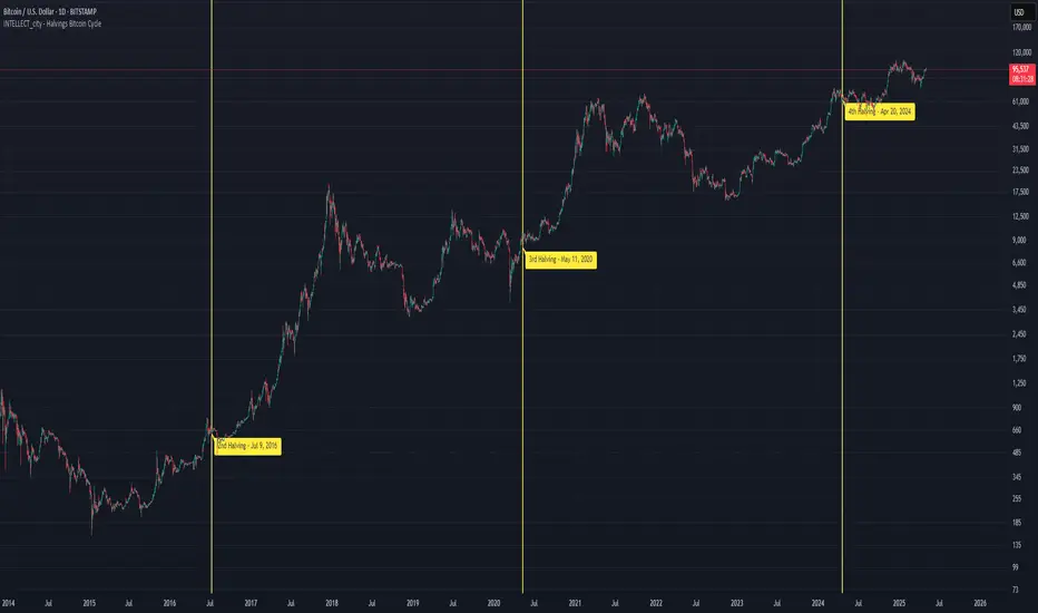
Overbought / Oversold Screener## Introduction
**The Versatile RSI and Stochastic Multi-Symbol Screener**
**Unlock a wealth of trading opportunities with this customizable screener, designed to pinpoint potential overbought and oversold conditions across 17 symbols, with alert support!**
## Description
This screener is suitable for tracking multiple instruments continuously.
With the screener, you can see the instant RSI or Stochastic values of the instruments you are tracking, and easily catch the moments when they are overbought / oversold according to your settings.
The purpose of the screener is to facilitate the continuous tracking of multiple instruments. The user can track up to 17 different instruments in different time intervals. If they wish, they can set an alarm and learn overbought oversold according to the values they set for the time interval of the instruments they are tracking.**
Key Features:
Comprehensive Analysis:
Monitors RSI and Stochastic values for 17 symbols simultaneously.
Automatically includes the current chart's symbol for seamless integration.
Supports multiple timeframes to uncover trends across different time horizons.
Personalized Insights:
Adjust overbought and oversold thresholds to align with your trading strategy.
Sort results by symbol, RSI, or Stochastic values to prioritize your analysis.
Choose between Automatic, Dark, or Light mode for optimal viewing comfort.
Dynamic Visual Cues:
Instantly highlights oversold and overbought symbols based on threshold levels.
Timely Alerts:
Stay informed of potential trading opportunities with alerts for multiple oversold or overbought symbols.
## Settings
### Display
**Timeframe**
The screener displays the values according to the selected timeframe. The default timeframe is "Chart". For example, if the timeframe is set to "15m" here, the screener will show the RSI and stochastic values for the 15-minute chart.
** Theme **
This setting is for changing the theme of the screener. You can set the theme to "Automatic", "Dark", or "Light", with "Automatic" being the default value. When the "Automatic" theme is selected, the screener appearance will also be automatically updated when you enable or disable dark mode from the TradingView settings.
** Position **
This option is for setting the position of the table on the chart. The default setting is "middle right". The available options are (top, middle, bottom)-(left, center, right).
** Sort By **
This option is for changing the sorting order of the table. The default setting is "RSI Descending". The available options are (Symbol, RSI, Stoch)-(Ascending, Descending).
It is important to note that the overbought and oversold coloring of the symbols may also change when the sorting order is changed. If RSI is selected as the sorting order, the symbols will be colored according to the overbought and oversold threshold values specified for RSI. Similarly, if Stoch is selected as the sorting order, the symbols will be colored according to the overbought and oversold threshold values specified for Stoch.
From this perspective, you can also think of the sorting order as a change in the main indicator.
### RSI / Stochastic
This area is for selecting the parameters of the RSI and stochastic indicators. You can adjust the values for "length", "overbought", and "oversold" for both indicators according to your needs. The screener will perform all RSI and stochastic calculations according to these settings. All coloring in the table will also be according to the overbought and oversold values in these settings.
### Symbols
The symbols to be tracked in the table are selected from here. Up to 16 symbols can be selected from here. Since the symbol in the chart is automatically added to the table, there will always be at least 1 symbol in the table. Note that the symbol in the chart is shown in the table with "(C)". For example, if SPX is open in the chart, it is shown as SPX(C) in the table.
## Alerts
The screener is capable of notifying you with an alarm if multiple symbols are overbought or oversold according to the values you specify along with the desired timeframe. This way, you can instantly learn if multiple symbols are overbought or oversold with one alarm, saving you time.

Optics Alert ZoneOptics Alert Zone shows price ranges for prices 17 days and 40 days ago. These can be adjusted based on asset class and volatility.
Bullish is when price is above 17 and 40 day.
Bearish is when price is below 17 and 40 day.
