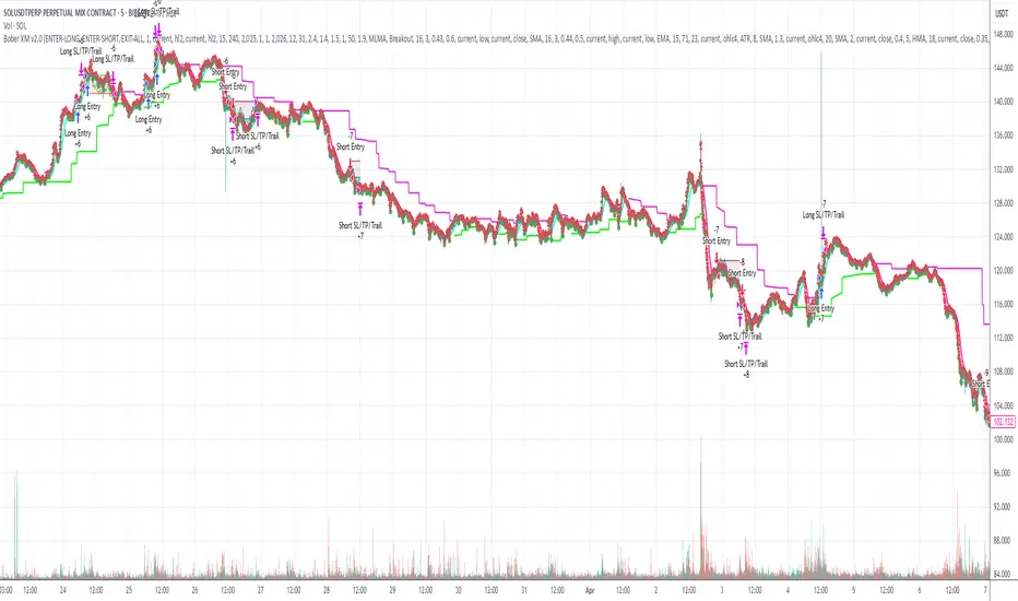
Bober XM v2.0# ₿ober XM v2.0 Trading Bot Documentation
**Developer's Note**: While our previous Bot 1.3.1 was removed due to guideline violations, this setback only fueled our determination to create something even better. Rising from this challenge, Bober XM 2.0 emerges not just as an update, but as a complete reimagining with multi-timeframe analysis, enhanced filters, and superior adaptability. This adversity pushed us to innovate further and deliver a strategy that's smarter, more agile, and more powerful than ever before. Challenges create opportunity - welcome to Cryptobeat's finest work yet.
## !!!!You need to tune it for your own pair and timeframe and retune it periodicaly!!!!!
## Overview
The ₿ober XM v2.0 is an advanced dual-channel trading bot with multi-timeframe analysis capabilities. It integrates multiple technical indicators, customizable risk management, and advanced order execution via webhook for automated trading. The bot's distinctive feature is its separate channel systems for long and short positions, allowing for asymmetric trade strategies that adapt to different market conditions across multiple timeframes.
### Key Features
- **Multi-Timeframe Analysis**: Analyze price data across multiple timeframes simultaneously
- **Dual Channel System**: Separate parameter sets for long and short positions
- **Advanced Entry Filters**: RSI, Volatility, Volume, Bollinger Bands, and KEMAD filters
- **Machine Learning Moving Average**: Adaptive prediction-based channels
- **Multiple Entry Strategies**: Breakout, Pullback, and Mean Reversion modes
- **Risk Management**: Customizable stop-loss, take-profit, and trailing stop settings
- **Webhook Integration**: Compatible with external trading bots and platforms
### Strategy Components
| Component | Description |
|---------|-------------|
| **Dual Channel Trading** | Uses either Keltner Channels or Machine Learning Moving Average (MLMA) with separate settings for long and short positions |
| **MLMA Implementation** | Machine learning algorithm that predicts future price movements and creates adaptive bands |
| **Pivot Point SuperTrend** | Trend identification and confirmation system based on pivot points |
| **Three Entry Strategies** | Choose between Breakout, Pullback, or Mean Reversion approaches |
| **Advanced Filter System** | Multiple customizable filters with multi-timeframe support to avoid false signals |
| **Custom Exit Logic** | Exits based on OBV crossover of its moving average combined with pivot trend changes |
### Note for Novice Users
This is a fully featured real trading bot and can be tweaked for any ticker — SOL is just an example. It follows this structure:
1. **Indicator** – gives the initial signal
2. **Entry strategy** – decides when to open a trade
3. **Exit strategy** – defines when to close it
4. **Trend confirmation** – ensures the trade follows the market direction
5. **Filters** – cuts out noise and avoids weak setups
6. **Risk management** – controls losses and protects your capital
To tune it for a different pair, you'll need to start from scratch:
1. Select the timeframe (candle size)
2. Turn off all filters and trend entry/exit confirmations
3. Choose a channel type, channel source and entry strategy
4. Adjust risk parameters
5. Tune long and short settings for the channel
6. Fine-tune the Pivot Point Supertrend and Main Exit condition OBV
This will generate a lot of signals and activity on the chart. Your next task is to find the right combination of filters and settings to reduce noise and tune it for profitability.
### Default Strategy values
Default values are tuned for: Symbol BITGET:SOLUSDT.P 5min candle
Filters are off by default: Try to play with it to understand how it works
## Configuration Guide
### General Settings
| Setting | Description | Default Value |
|---------|-------------|---------------|
| **Long Positions** | Enable or disable long trades | Enabled |
| **Short Positions** | Enable or disable short trades | Enabled |
| **Risk/Reward Area** | Visual display of stop-loss and take-profit zones | Enabled |
| **Long Entry Source** | Price data used for long entry signals | hl2 (High+Low/2) |
| **Short Entry Source** | Price data used for short entry signals | hl2 (High+Low/2) |
The bot allows you to trade long positions, short positions, or both simultaneously. Each direction has its own set of parameters, allowing for fine-tuned strategies that recognize the asymmetric nature of market movements.
### Multi-Timeframe Settings
1. **Enable Multi-Timeframe Analysis**: Toggle 'Enable Multi-Timeframe Analysis' in the Multi-Timeframe Settings section
2. **Configure Timeframes**: Set appropriate higher timeframes based on your trading style:
- Timeframe 1: Default is now 15 minutes (intraday confirmation)
- Timeframe 2: Default is 4 hours (trend direction)
3. **Select Sources per Indicator**: For each indicator (RSI, KEMAD, Volume, etc.), choose:
- The desired timeframe (current, mtf1, or mtf2)
- The appropriate price type (open, high, low, close, hl2, hlc3, ohlc4)
### Entry Strategies
- **Breakout**: Enter when price breaks above/below the channel
- **Pullback**: Enter when price pulls back to the channel
- **Mean Reversion**: Enter when price is extended from the channel
You can enable different strategies for long and short positions.
### Core Components
### Risk Management
- **Position Size**: Control risk with percentage-based position sizing
- **Stop Loss Options**:
- Fixed: Set a specific price or percentage from entry
- ATR-based: Dynamic stop-loss based on market volatility
- Swing: Uses recent swing high/low points
- **Take Profit**: Multiple targets with percentage allocation
- **Trailing Stop**: Dynamic stop that follows price movement
## Advanced Usage Strategies
### Moving Average Type Selection Guide
- **SMA**: More stable in choppy markets, good for higher timeframes
- **EMA/WMA**: More responsive to recent price changes, better for entry signals
- **VWMA**: Adds volume weighting for stronger trends, use with Volume filter
- **HMA**: Balance between responsiveness and noise reduction, good for volatile markets
### Multi-Timeframe Strategy Approaches
- **Trend Confirmation**: Use higher timeframe RSI (mtf2) for overall trend, current timeframe for entries
- **Entry Precision**: Use KEMAD on current timeframe with volume filter on mtf1
- **False Signal Reduction**: Apply RSI filter on mtf1 with strict KEMAD settings
### Market Condition Optimization
| Market Condition | Recommended Settings |
|------------------|----------------------|
| **Trending** | Use Breakout strategy with KEMAD filter on higher timeframe |
| **Ranging** | Use Mean Reversion with strict RSI filter (mtf1) |
| **Volatile** | Increase ATR multipliers, use HMA for moving averages |
| **Low Volatility** | Decrease noise parameters, use pullback strategy |
## Webhook Integration
The strategy features a professional webhook system that allows direct connectivity to your exchange or trading platform of choice through third-party services like 3commas, Alertatron, or Autoview.
The webhook payload includes all necessary parameters for automated execution:
- Entry price and direction
- Stop loss and take profit levels
- Position size
- Custom identifier for webhook routing
## Performance Optimization Tips
1. **Start with Defaults**: Begin with the default settings for your timeframe before customizing
2. **Adjust One Component at a Time**: Make incremental changes and test the impact
3. **Match MA Types to Market Conditions**: Use appropriate moving average types based on the Market Condition Optimization table
4. **Timeframe Synergy**: Create logical relationships between timeframes (e.g., 5min chart with 15min and 4h higher timeframes)
5. **Periodic Retuning**: Markets evolve - regularly review and adjust parameters
## Common Setups
### Crypto Trend-Following
- MLMA with EMA or HMA
- Higher RSI thresholds (75/25)
- KEMAD filter on mtf1
- Breakout entry strategy
### Stock Swing Trading
- MLMA with SMA for stability
- Volume filter with higher threshold
- KEMAD with increased filter order
- Pullback entry strategy
### Forex Scalping
- MLMA with WMA and lower noise parameter
- RSI filter on current timeframe
- Use highest timeframe for trend direction only
- Mean Reversion strategy
## Webhook Configuration
- **Benefits**:
- Automated trade execution without manual intervention
- Immediate response to market conditions
- Consistent execution of your strategy
- **Implementation Notes**:
- Requires proper webhook configuration on your exchange or platform
- Test thoroughly with small position sizes before full deployment
- Consider latency between signal generation and execution
### Backtesting Period
Define a specific historical period to evaluate the bot's performance:
| Setting | Description | Default Value |
|---------|-------------|---------------|
| **Start Date** | Beginning of backtest period | January 1, 2025 |
| **End Date** | End of backtest period | December 31, 2026 |
- **Best Practice**: Test across different market conditions (bull markets, bear markets, sideways markets)
- **Limitation**: Past performance doesn't guarantee future results
## Entry and Exit Strategies
### Dual-Channel System
A key innovation of the Bober XM is its dual-channel approach:
- **Independent Parameters**: Each trade direction has its own channel settings
- **Asymmetric Trading**: Recognizes that markets often behave differently in uptrends versus downtrends
- **Optimized Performance**: Fine-tune settings for both bullish and bearish conditions
This approach allows the bot to adapt to the natural asymmetry of markets, where uptrends often develop gradually while downtrends can be sharp and sudden.
### Channel Types
#### 1. Keltner Channels
Traditional volatility-based channels using EMA and ATR:
| Setting | Long Default | Short Default |
|---------|--------------|---------------|
| **EMA Length** | 37 | 20 |
| **ATR Length** | 13 | 17 |
| **Multiplier** | 1.4 | 1.9 |
| **Source** | low | high |
- **Strengths**:
- Reliable in trending markets
- Less prone to whipsaws than Bollinger Bands
- Clear visual representation of volatility
- **Weaknesses**:
- Can lag during rapid market changes
- Less effective in choppy, non-trending markets
#### 2. Machine Learning Moving Average (MLMA)
Advanced predictive model using kernel regression (RBF kernel):
| Setting | Description | Options |
|---------|-------------|--------|
| **Source MA** | Price data used for MA calculations | Any price source (low/high/close/etc.) |
| **Moving Average Type** | Type of MA algorithm for calculations | SMA, EMA, WMA, VWMA, RMA, HMA |
| **Trend Source** | Price data used for trend determination | Any price source (close default) |
| **Window Size** | Historical window for MLMA calculations | 5+ (default: 16) |
| **Forecast Length** | Number of bars to forecast ahead | 1+ (default: 3) |
| **Noise Parameter** | Controls smoothness of prediction | 0.01+ (default: ~0.43) |
| **Band Multiplier** | Multiplier for channel width | 0.1+ (default: 0.5-0.6) |
- **Strengths**:
- Predictive rather than reactive
- Adapts quickly to changing market conditions
- Better at identifying trend reversals early
- **Weaknesses**:
- More computationally intensive
- Requires careful parameter tuning
- Can be sensitive to input data quality
### Entry Strategies
| Strategy | Description | Ideal Market Conditions |
|----------|-------------|-------------------------|
| **Breakout** | Enters when price breaks through channel bands, indicating strong momentum | High volatility, emerging trends |
| **Pullback** | Enters when price retraces to the middle band after testing extremes | Established trends with regular pullbacks |
| **Mean Reversion** | Enters at channel extremes, betting on a return to the mean | Range-bound or oscillating markets |
#### Breakout Strategy (Default)
- **Implementation**: Enters long when price crosses above the upper band, short when price crosses below the lower band
- **Strengths**: Captures strong momentum moves, performs well in trending markets
- **Weaknesses**: Can lead to late entries, higher risk of false breakouts
- **Optimization Tips**:
- Increase channel multiplier for fewer but more reliable signals
- Combine with volume confirmation for better accuracy
#### Pullback Strategy
- **Implementation**: Enters long when price pulls back to middle band during uptrend, short during downtrend pullbacks
- **Strengths**: Better entry prices, lower risk, higher probability setups
- **Weaknesses**: Misses some strong moves, requires clear trend identification
- **Optimization Tips**:
- Use with trend filters to confirm overall direction
- Adjust middle band calculation for market volatility
#### Mean Reversion Strategy
- **Implementation**: Enters long at lower band, short at upper band, expecting price to revert to the mean
- **Strengths**: Excellent entry prices, works well in ranging markets
- **Weaknesses**: Dangerous in strong trends, can lead to fighting the trend
- **Optimization Tips**:
- Implement strong trend filters to avoid counter-trend trades
- Use smaller position sizes due to higher risk nature
### Confirmation Indicators
#### Pivot Point SuperTrend
Combines pivot points with ATR-based SuperTrend for trend confirmation:
| Setting | Default Value |
|---------|---------------|
| **Pivot Period** | 25 |
| **ATR Factor** | 2.2 |
| **ATR Period** | 41 |
- **Function**: Identifies significant market turning points and confirms trend direction
- **Implementation**: Requires price to respect the SuperTrend line for trade confirmation
#### Weighted Moving Average (WMA)
Provides additional confirmation layer for entries:
| Setting | Default Value |
|---------|---------------|
| **Period** | 15 |
| **Source** | ohlc4 (average of Open, High, Low, Close) |
- **Function**: Confirms trend direction and filters out low-quality signals
- **Implementation**: Price must be above WMA for longs, below for shorts
### Exit Strategies
#### On-Balance Volume (OBV) Based Exits
Uses volume flow to identify potential reversals:
| Setting | Default Value |
|---------|---------------|
| **Source** | ohlc4 |
| **MA Type** | HMA (Options: SMA, EMA, WMA, RMA, VWMA, HMA) |
| **Period** | 22 |
- **Function**: Identifies divergences between price and volume to exit before reversals
- **Implementation**: Exits when OBV crosses its moving average in the opposite direction
- **Customizable MA Type**: Different MA types provide varying sensitivity to OBV changes:
- **SMA**: Traditional simple average, equal weight to all periods
- **EMA**: More weight to recent data, responds faster to price changes
- **WMA**: Weighted by recency, smoother than EMA
- **RMA**: Similar to EMA but smoother, reduces noise
- **VWMA**: Factors in volume, helpful for OBV confirmation
- **HMA**: Reduces lag while maintaining smoothness (default)
#### ADX Exit Confirmation
Uses Average Directional Index to confirm trend exhaustion:
| Setting | Default Value |
|---------|---------------|
| **ADX Threshold** | 35 |
| **ADX Smoothing** | 60 |
| **DI Length** | 60 |
- **Function**: Confirms trend weakness before exiting positions
- **Implementation**: Requires ADX to drop below threshold or DI lines to cross
## Filter System
### RSI Filter
- **Function**: Controls entries based on momentum conditions
- **Parameters**:
- Period: 15 (default)
- Overbought level: 71
- Oversold level: 23
- Multi-timeframe support: Current, MTF1 (15min), or MTF2 (4h)
- Customizable price source (open, high, low, close, hl2, hlc3, ohlc4)
- **Implementation**: Blocks long entries when RSI > overbought, short entries when RSI < oversold
### Volatility Filter
- **Function**: Prevents trading during excessive market volatility
- **Parameters**:
- Measure: ATR (Average True Range)
- Period: Customizable (default varies by timeframe)
- Threshold: Adjustable multiplier
- Multi-timeframe support
- Customizable price source
- **Implementation**: Blocks trades when current volatility exceeds threshold × average volatility
### Volume Filter
- **Function**: Ensures adequate market liquidity for trades
- **Parameters**:
- Threshold: 0.4× average (default)
- Measurement period: 5 (default)
- Moving average type: Customizable (HMA default)
- Multi-timeframe support
- Customizable price source
- **Implementation**: Requires current volume to exceed threshold × average volume
### Bollinger Bands Filter
- **Function**: Controls entries based on price relative to statistical boundaries
- **Parameters**:
- Period: Customizable
- Standard deviation multiplier: Adjustable
- Moving average type: Customizable
- Multi-timeframe support
- Customizable price source
- **Implementation**: Can require price to be within bands or breaking out of bands depending on strategy
### KEMAD Filter (Kalman EMA Distance)
- **Function**: Advanced trend confirmation using Kalman filter algorithm
- **Parameters**:
- Process Noise: 0.35 (controls smoothness)
- Measurement Noise: 24 (controls reactivity)
- Filter Order: 6 (higher = more smoothing)
- ATR Length: 8 (for bandwidth calculation)
- Upper Multiplier: 2.0 (for long signals)
- Lower Multiplier: 2.7 (for short signals)
- Multi-timeframe support
- Customizable visual indicators
- **Implementation**: Generates signals based on price position relative to Kalman-filtered EMA bands
## Risk Management System
### Position Sizing
Automatically calculates position size based on account equity and risk parameters:
| Setting | Default Value |
|---------|---------------|
| **Risk % of Equity** | 50% |
- **Implementation**:
- Position size = (Account equity × Risk %) ÷ (Entry price × Stop loss distance)
- Adjusts automatically based on volatility and stop placement
- **Best Practices**:
- Start with lower risk percentages (1-2%) until strategy is proven
- Consider reducing risk during high volatility periods
### Stop-Loss Methods
Multiple stop-loss calculation methods with separate configurations for long and short positions:
| Method | Description | Configuration |
|--------|-------------|---------------|
| **ATR-Based** | Dynamic stops based on volatility | ATR Period: 14, Multiplier: 2.0 |
| **Percentage** | Fixed percentage from entry | Long: 1.5%, Short: 1.5% |
| **PIP-Based** | Fixed currency unit distance | 10.0 pips |
- **Implementation Notes**:
- ATR-based stops adapt to changing market volatility
- Percentage stops maintain consistent risk exposure
- PIP-based stops provide precise control in stable markets
### Trailing Stops
Locks in profits by adjusting stop-loss levels as price moves favorably:
| Setting | Default Value |
|---------|---------------|
| **Stop-Loss %** | 1.5% |
| **Activation Threshold** | 2.1% |
| **Trailing Distance** | 1.4% |
- **Implementation**:
- Initial stop remains fixed until profit reaches activation threshold
- Once activated, stop follows price at specified distance
- Locks in profit while allowing room for normal price fluctuations
### Risk-Reward Parameters
Defines the relationship between risk and potential reward:
| Setting | Default Value |
|---------|---------------|
| **Risk-Reward Ratio** | 1.4 |
| **Take Profit %** | 2.4% |
| **Stop-Loss %** | 1.5% |
- **Implementation**:
- Take profit distance = Stop loss distance × Risk-reward ratio
- Higher ratios require fewer winning trades for profitability
- Lower ratios increase win rate but reduce average profit
### Filter Combinations
The strategy allows for simultaneous application of multiple filters:
- **Recommended Combinations**:
- Trending markets: RSI + KEMAD filters
- Ranging markets: Bollinger Bands + Volatility filters
- All markets: Volume filter as minimum requirement
- **Performance Impact**:
- Each additional filter reduces the number of trades
- Quality of remaining trades typically improves
- Optimal combination depends on market conditions and timeframe
### Multi-Timeframe Filter Applications
| Filter Type | Current Timeframe | MTF1 (15min) | MTF2 (4h) |
|-------------|-------------------|-------------|------------|
| RSI | Quick entries/exits | Intraday trend | Overall trend |
| Volume | Immediate liquidity | Sustained support | Market participation |
| Volatility | Entry timing | Short-term risk | Regime changes |
| KEMAD | Precise signals | Trend confirmation | Major reversals |
## Visual Indicators and Chart Analysis
The bot provides comprehensive visual feedback on the chart:
- **Channel Bands**: Keltner or MLMA bands showing potential support/resistance
- **Pivot SuperTrend**: Colored line showing trend direction and potential reversal points
- **Entry/Exit Markers**: Annotations showing actual trade entries and exits
- **Risk/Reward Zones**: Visual representation of stop-loss and take-profit levels
These visual elements allow for:
- Real-time strategy assessment
- Post-trade analysis and optimization
- Educational understanding of the strategy logic
## Implementation Guide
### TradingView Setup
1. Load the script in TradingView Pine Editor
2. Apply to your preferred chart and timeframe
3. Adjust parameters based on your trading preferences
4. Enable alerts for webhook integration
### Webhook Integration
1. Configure webhook URL in TradingView alerts
2. Set up receiving endpoint on your trading platform
3. Define message format matching the bot's output
4. Test with small position sizes before full deployment
### Optimization Process
1. Backtest across different market conditions
2. Identify parameter sensitivity through multiple tests
3. Focus on risk management parameters first
4. Fine-tune entry/exit conditions based on performance metrics
5. Validate with out-of-sample testing
## Performance Considerations
### Strengths
- Adaptability to different market conditions through dual channels
- Multiple layers of confirmation reducing false signals
- Comprehensive risk management protecting capital
- Machine learning integration for predictive edge
### Limitations
- Complex parameter set requiring careful optimization
- Potential over-optimization risk with so many variables
- Computational intensity of MLMA calculations
- Dependency on proper webhook configuration for execution
### Best Practices
- Start with conservative risk settings (1-2% of equity)
- Test thoroughly in demo environment before live trading
- Monitor performance regularly and adjust parameters
- Consider market regime changes when evaluating results
## Conclusion
The ₿ober XM v2.0 represents a significant evolution in trading strategy design, combining traditional technical analysis with machine learning elements and multi-timeframe analysis. The core strength of this system lies in its adaptability and recognition of market asymmetry.
### Market Asymmetry and Adaptive Approach
The strategy acknowledges a fundamental truth about markets: bullish and bearish phases behave differently and should be treated as distinct environments. The dual-channel system with separate parameters for long and short positions directly addresses this asymmetry, allowing for optimized performance regardless of market direction.
### Targeted Backtesting Philosophy
It's counterproductive to run backtests over excessively long periods. Markets evolve continuously, and strategies that worked in previous market regimes may be ineffective in current conditions. Instead:
- Test specific market phases separately (bull markets, bear markets, range-bound periods)
- Regularly re-optimize parameters as market conditions change
- Focus on recent performance with higher weight than historical results
- Test across multiple timeframes to ensure robustness
### Multi-Timeframe Analysis as a Game-Changer
The integration of multi-timeframe analysis fundamentally transforms the strategy's effectiveness:
- **Increased Safety**: Higher timeframe confirmations reduce false signals and improve trade quality
- **Context Awareness**: Decisions made with awareness of larger trends reduce adverse entries
- **Adaptable Precision**: Apply strict filters on lower timeframes while maintaining awareness of broader conditions
- **Reduced Noise**: Higher timeframe data naturally filters market noise that can trigger poor entries
The ₿ober XM v2.0 provides traders with a framework that acknowledges market complexity while offering practical tools to navigate it. With proper setup, realistic expectations, and attention to changing market conditions, it delivers a sophisticated approach to systematic trading that can be continuously refined and optimized.
Cari dalam skrip untuk "17个交易日涨幅第一的股票(非新股)有哪些"
Kernel Regression Bands SuiteMulti-Kernel Regression Bands
A versatile indicator that applies kernel regression smoothing to price data, then dynamically calculates upper and lower bands using a wide variety of deviation methods. This tool is designed to help traders identify trend direction, volatility, and potential reversal zones with customizable visual styles.
Key Features
Multiple Kernel Types: Choose from 17+ kernel regression styles (Gaussian, Laplace, Epanechnikov, etc.) for smoothing.
Flexible Band Calculation: Select from 12+ deviation types including Standard Deviation, Mean/Median Absolute Deviation, Exponential, True Range, Hull, Parabolic SAR, Quantile, and more.
Adaptive Bands: Bands are calculated around the kernel regression line, with a user-defined multiplier.
Signal Logic: Trend state is determined by crossovers/crossunders of price and bands, coloring the regression line and band fills accordingly.
Custom Color Modes: Six unique color palettes for visual clarity and personal preference.
Highly Customizable Inputs: Adjust kernel type, lookback, deviation method, band source, and more.
How to Use
Trend Identification: The regression line changes color based on the detected trend (up/down)
Volatility Zones: Bands expand/contract with volatility, helping spot breakouts or mean-reversion opportunities.
Visual Styling: Use color modes to match your chart theme or highlight specific market states.
Credits:
Kernel regression logic adapted from:
ChartPrime | Multi-Kernel-Regression-ChartPrime (Link in the script)
Disclaimer
This script is for educational and informational purposes only. Not financial advice. Use at your own risk.

AllCandlestickPatternsLibraryAll Candlestick Patterns Library
The Candlestick Patterns Library is a Pine Script (version 6) library extracted from the All Candlestick Patterns indicator. It provides a comprehensive set of functions to calculate candlestick properties, detect market trends, and identify various candlestick patterns (bullish, bearish, and neutral). The library is designed for reusability, enabling TradingView users to incorporate pattern detection into their own scripts, such as indicators or strategies.
The library is organized into three main sections:
Trend Detection: Functions to determine market trends (uptrend or downtrend) based on user-defined rules.
Candlestick Property Calculations: A function to compute core properties of a candlestick, such as body size, shadow lengths, and doji characteristics.
Candlestick Pattern Detection: Functions to detect specific candlestick patterns, each returning a tuple with detection status, pattern name, type, and description.
Library Structure
1. Trend Detection
This section includes the detectTrend function, which identifies whether the market is in an uptrend or downtrend based on user-specified rules, such as the relationship between the closing price and Simple Moving Averages (SMAs).
Function: detectTrend
Parameters:
downTrend (bool): Initial downtrend condition.
upTrend (bool): Initial uptrend condition.
trendRule (string): The rule for trend detection ("SMA50" or "SMA50, SMA200").
p_close (float): Current closing price.
sma50 (float): Simple Moving Average over 50 periods.
sma200 (float): Simple Moving Average over 200 periods.
Returns: A tuple indicating the detected trend.
Logic:
If trendRule is "SMA50", a downtrend is detected when p_close < sma50, and an uptrend when p_close > sma50.
If trendRule is "SMA50, SMA200", a downtrend is detected when p_close < sma50 and sma50 < sma200, and an uptrend when p_close > sma50 and sma50 > sma200.
2. Candlestick Property Calculations
This section includes the calculateCandleProperties function, which computes essential properties of a candlestick based on OHLC (Open, High, Low, Close) data and configuration parameters.
Function: calculateCandleProperties
Parameters:
p_open (float): Candlestick open price.
p_close (float): Candlestick close price.
p_high (float): Candlestick high price.
p_low (float): Candlestick low price.
bodyAvg (float): Average body size (e.g., from EMA of body sizes).
shadowPercent (float): Minimum shadow size as a percentage of body size.
shadowEqualsPercent (float): Tolerance for equal shadows in doji detection.
dojiBodyPercent (float): Maximum body size as a percentage of range for doji detection.
Returns: A tuple containing 17 properties:
C_BodyHi (float): Higher of open or close price.
C_BodyLo (float): Lower of open or close price.
C_Body (float): Body size (difference between C_BodyHi and C_BodyLo).
C_SmallBody (bool): True if body size is below bodyAvg.
C_LongBody (bool): True if body size is above bodyAvg.
C_UpShadow (float): Upper shadow length (p_high - C_BodyHi).
C_DnShadow (float): Lower shadow length (C_BodyLo - p_low).
C_HasUpShadow (bool): True if upper shadow exceeds shadowPercent of body.
C_HasDnShadow (bool): True if lower shadow exceeds shadowPercent of body.
C_WhiteBody (bool): True if candle is bullish (p_open < p_close).
C_BlackBody (bool): True if candle is bearish (p_open > p_close).
C_Range (float): Candlestick range (p_high - p_low).
C_IsInsideBar (bool): True if current candle body is inside the previous candle's body.
C_BodyMiddle (float): Midpoint of the candle body.
C_ShadowEquals (bool): True if upper and lower shadows are equal within shadowEqualsPercent.
C_IsDojiBody (bool): True if body size is small relative to range (C_Body <= C_Range * dojiBodyPercent / 100).
C_Doji (bool): True if the candle is a doji (C_IsDojiBody and C_ShadowEquals).
Purpose: These properties are used by pattern detection functions to evaluate candlestick formations.
3. Candlestick Pattern Detection
This section contains functions to detect specific candlestick patterns, each returning a tuple . The patterns are categorized as bullish, bearish, or neutral, and include detailed descriptions for use in tooltips or alerts.
Supported Patterns
The library supports the following candlestick patterns, grouped by type:
Bullish Patterns:
Rising Window: A two-candle continuation pattern in an uptrend with a price gap between the first candle's high and the second candle's low.
Rising Three Methods: A five-candle continuation pattern with a long green candle, three short red candles, and another long green candle.
Tweezer Bottom: A two-candle reversal pattern in a downtrend with nearly identical lows.
Upside Tasuki Gap: A three-candle continuation pattern in an uptrend with a gap between the first two green candles and a red candle closing partially into the gap.
Doji Star (Bullish): A two-candle reversal pattern in a downtrend with a long red candle followed by a doji gapping down.
Morning Doji Star: A three-candle reversal pattern with a long red candle, a doji gapping down, and a long green candle.
Piercing: A two-candle reversal pattern in a downtrend with a red candle followed by a green candle closing above the midpoint of the first.
Hammer: A single-candle reversal pattern in a downtrend with a small body and a long lower shadow.
Inverted Hammer: A single-candle reversal pattern in a downtrend with a small body and a long upper shadow.
Morning Star: A three-candle reversal pattern with a long red candle, a short candle gapping down, and a long green candle.
Marubozu White: A single-candle pattern with a long green body and minimal shadows.
Dragonfly Doji: A single-candle reversal pattern in a downtrend with a doji where open and close are at the high.
Harami Cross (Bullish): A two-candle reversal pattern in a downtrend with a long red candle followed by a doji inside its body.
Harami (Bullish): A two-candle reversal pattern in a downtrend with a long red candle followed by a small green candle inside its body.
Long Lower Shadow: A single-candle pattern with a long lower shadow indicating buyer strength.
Three White Soldiers: A three-candle reversal pattern with three long green candles in a downtrend.
Engulfing (Bullish): A two-candle reversal pattern in a downtrend with a small red candle followed by a larger green candle engulfing it.
Abandoned Baby (Bullish): A three-candle reversal pattern with a long red candle, a doji gapping down, and a green candle gapping up.
Tri-Star (Bullish): A three-candle reversal pattern with three doji candles in a downtrend, with gaps between them.
Kicking (Bullish): A two-candle reversal pattern with a bearish marubozu followed by a bullish marubozu gapping up.
Bearish Patterns:
On Neck: A two-candle continuation pattern in a downtrend with a long red candle followed by a short green candle closing near the first candle's low.
Falling Window: A two-candle continuation pattern in a downtrend with a price gap between the first candle's low and the second candle's high.
Falling Three Methods: A five-candle continuation pattern with a long red candle, three short green candles, and another long red candle.
Tweezer Top: A two-candle reversal pattern in an uptrend with nearly identical highs.
Dark Cloud Cover: A two-candle reversal pattern in an uptrend with a green candle followed by a red candle opening above the high and closing below the midpoint.
Downside Tasuki Gap: A three-candle continuation pattern in a downtrend with a gap between the first two red candles and a green candle closing partially into the gap.
Evening Doji Star: A three-candle reversal pattern with a long green candle, a doji gapping up, and a long red candle.
Doji Star (Bearish): A two-candle reversal pattern in an uptrend with a long green candle followed by a doji gapping up.
Hanging Man: A single-candle reversal pattern in an uptrend with a small body and a long lower shadow.
Shooting Star: A single-candle reversal pattern in an uptrend with a small body and a long upper shadow.
Evening Star: A three-candle reversal pattern with a long green candle, a short candle gapping up, and a long red candle.
Marubozu Black: A single-candle pattern with a long red body and minimal shadows.
Gravestone Doji: A single-candle reversal pattern in an uptrend with a doji where open and close are at the low.
Harami Cross (Bearish): A two-candle reversal pattern in an uptrend with a long green candle followed by a doji inside its body.
Harami (Bearish): A two-candle reversal pattern in an uptrend with a long green candle followed by a small red candle inside its body.
Long Upper Shadow: A single-candle pattern with a long upper shadow indicating seller strength.
Three Black Crows: A three-candle reversal pattern with three long red candles in an uptrend.
Engulfing (Bearish): A two-candle reversal pattern in an uptrend with a small green candle followed by a larger red candle engulfing it.
Abandoned Baby (Bearish): A three-candle reversal pattern with a long green candle, a doji gapping up, and a red candle gapping down.
Tri-Star (Bearish): A three-candle reversal pattern with three doji candles in an uptrend, with gaps between them.
Kicking (Bearish): A two-candle reversal pattern with a bullish marubozu followed by a bearish marubozu gapping down.
Neutral Patterns:
Doji: A single-candle pattern with a very small body, indicating indecision.
Spinning Top White: A single-candle pattern with a small green body and long upper and lower shadows, indicating indecision.
Spinning Top Black: A single-candle pattern with a small red body and long upper and lower shadows, indicating indecision.
Pattern Detection Functions
Each pattern detection function evaluates specific conditions based on candlestick properties (from calculateCandleProperties) and trend conditions (from detectTrend). The functions return:
detected (bool): True if the pattern is detected.
name (string): The name of the pattern (e.g., "On Neck").
type (string): The pattern type ("Bullish", "Bearish", or "Neutral").
description (string): A detailed description of the pattern for use in tooltips or alerts.
For example, the detectOnNeckBearish function checks for a bearish On Neck pattern by verifying a downtrend, a long red candle followed by a short green candle, and specific price relationships.
Usage Example
To use the library in a TradingView indicator, you can import it and call its functions as shown below:
//@version=6
indicator("Candlestick Pattern Detector", overlay=true)
import CandlestickPatternsLibrary as cp
// Calculate SMA for trend detection
sma50 = ta.sma(close, 50)
sma200 = ta.sma(close, 200)
= cp.detectTrend(true, true, "SMA50", close, sma50, sma200)
// Calculate candlestick properties
bodyAvg = ta.ema(math.max(close, open) - math.min(close, open), 14)
= cp.calculateCandleProperties(open, close, high, low, bodyAvg, 5.0, 100.0, 5.0)
// Detect a pattern (e.g., On Neck Bearish)
= cp.detectOnNeckBearish(downTrend, blackBody, longBody, whiteBody, open, close, low, bodyAvg, smallBody, candleRange)
if onNeckDetected
label.new(bar_index, low, onNeckName, style=label.style_label_up, color=color.red, textcolor=color.white, tooltip=onNeckDesc)
// Detect another pattern (e.g., Piercing Bullish)
= cp.detectPiercingBullish(downTrend, blackBody, longBody, whiteBody, open, low, close, bodyMiddle)
if piercingDetected
label.new(bar_index, low, piercingName, style=label.style_label_up, color=color.blue, textcolor=color.white, tooltip=piercingDesc)
Steps in the Example
Import the Library: Use import CandlestickPatternsLibrary as cp to access the library's functions.
Calculate Trend: Use detectTrend to determine the market trend based on SMA50 or SMA50/SMA200 rules.
Calculate Candlestick Properties: Use calculateCandleProperties to compute properties like body size, shadow lengths, and doji status.
Detect Patterns: Call specific pattern detection functions (e.g., detectOnNeckBearish, detectPiercingBullish) and use the returned values to display labels or alerts.
Visualize Patterns: Use label.new to display detected patterns on the chart with their names, types, and descriptions.
Key Features
Modularity: The library is designed as a standalone module, making it easy to integrate into other Pine Script projects.
Comprehensive Pattern Coverage: Supports over 40 candlestick patterns, covering bullish, bearish, and neutral formations.
Detailed Documentation: Each function includes comments with @param and @returns annotations for clarity.
Reusability: Can be used in indicators, strategies, or alerts by importing the library and calling its functions.
Extracted from All Candlestick Patterns: The library is derived from the All Candlestick Patterns indicator, ensuring it inherits a well-tested foundation for pattern detection.
Notes for Developers
Pine Script Version: The library uses Pine Script version 6, as specified by //@version=6.
Parameter Naming: Parameters use prefixes like p_ (e.g., p_open, p_close) to avoid conflicts with built-in variables.
Error Handling: The library has been fixed to address issues like undeclared identifiers (C_SmallBody, C_Range), unused arguments (factor), and improper comment formatting.
Testing: Developers should test the library in TradingView to ensure patterns are detected correctly under various market conditions.
Customization: Users can adjust parameters like bodyAvg, shadowPercent, shadowEqualsPercent, and dojiBodyPercent in calculateCandleProperties to fine-tune pattern detection sensitivity.
Conclusion
The Candlestick Patterns Library, extracted from the All Candlestick Patterns indicator, is a powerful tool for traders and developers looking to implement candlestick pattern detection in TradingView. Its modular design, comprehensive pattern support, and detailed documentation make it an ideal choice for building custom indicators or strategies. By leveraging the library's functions, users can analyze market trends, compute candlestick properties, and detect a wide range of patterns to inform their trading decisions.

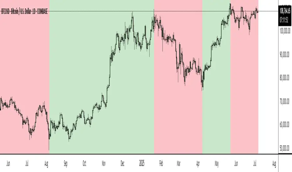
BTC Markup/Markdown Zones by Koenigsegg📈 BTC Markup/Markdown Zones
A handcrafted indicator designed to mark Bitcoin's most critical High Time Frame (HTF) structure shifts. This tool overlays true institutional-level Markup and Markdown Zones, selected manually after deep market review. Whether you're testing strategies or actively trading, this tool gives you the bigger picture at all times.
🔍 Key Features:
✅ HTF Markup & Markdown Zones
Every zone is manually selected — no indicators, no repainting. Just raw market history and real structure.
✅ Two Display Modes
• Background Zones — soft overlays with low opacity for visual context — with the option to increase opacity manually if desired.
• Start Candle Highlight — sharply highlighted candle marking the final pivot before a macro reversal.
✅ Custom Color Controls (Style Tab)
All visual styling lives in the Style tab, with clearly labeled fields:
• Markup Zone
• Markdown Zone
• Start Candle Highlight Markup
• Start Candle Highlight Markdown
✅ Minimal Input Section
Just one toggle: display mode. Everything else is kept clean and intuitive.
🧠 Purpose:
This script is made for any timeframe:
• Zoom into lower timeframes to know whether you're trading inside a Markup or Markdown
• Use it during strategy testing for true structural awareness
📅 Handpicked Macro Turning Points:
Each zone originates from a manually confirmed candle — the last meaningful candle before a shift in control between bulls and bears:
• FRI 19 AUG 2011 12PM – MARK DOWN
• THU 20 OCT 2011 12AM – MARK UP
• WED 10 APR 2013 12PM – MARK DOWN
• FRI 12 APR 2013 12PM – MARK UP
• SAT 30 NOV 2013 12AM – MARK DOWN
• WED 14 JAN 2015 12PM – MARK UP
• SUN 17 DEC 2017 12PM – MARK DOWN
• SAT 15 DEC 2018 12PM – MARK UP
• WED 14 APR 2021 4AM – MARK DOWN
• TUE 22 JUN 2021 12PM – MARK UP
• WED 10 NOV 2021 12PM – MARK DOWN
• MON 21 NOV 2022 8PM – MARK UP
• THU 14 MAR 2024 4AM – MARK DOWN
• MON 5 AUG 2024 12PM – MARK UP
• MON 20 JAN 2025 4AM – MARK DOWN
💡 Zones are manually updated by me after each new confirmed Markup or Markdown.
🧬 Fractal Structure for MTF Systems
Price is fractal — meaning the same principles of structure repeat across all timeframes. In Version 2, this tool evolves by introducing manually selected sub-zones inside each High Time Frame (HTF) Markup or Markdown. These sub-zones reflect Medium Timeframe (MTF) structure shifts, offering precision for traders who operate on both intraday and swing levels.
This makes the indicator ideal for low timeframe (LTF) Markup/Markdown awareness — whether you're managing 15m entries or building multi-timeframe confluence systems.
No auto-zones. No guesswork. Just clean, intentional structure division within the broader trend, handpicked for maximum clarity and edge.
💡 Pro Tip:
When price is inside a Markup Zone, shorting becomes riskier — you're trading against a macro bullish structure.
When inside a Markdown Zone, longing becomes riskier — you're fighting against confirmed bearish momentum.
Use this tool to stay aligned with the broader move, especially when zoomed into smaller timeframes or managing entries/exits during intraday setups.
📈 Markup Phase – Bullish Sentiment
Definition: A period where price makes higher highs and higher lows — the uptrend is in full force.
Why sentiment is bullish:
- Institutions and smart money are already positioned long.
- Public/institutional demand drives prices up.
- Momentum is supported by positive news, breakouts, and FOMO.
- Higher highs confirm buyers are in control.
📉 Markdown Phase – Bearish Sentiment
Definition: A period where price makes lower lows and lower highs — clear downtrend.
Why sentiment is bearish:
- Distribution has already occurred, and supply outweighs demand.
- Smart money is short or sidelined, waiting for deeper prices.
- Panic selling or trend-following traders add downside momentum.
- Lower lows confirm sellers are in control.
❌ Trading Against the Trend — Consequences:
-Reduced Probability of Success
-You’re fighting the dominant flow. Most participants are pushing in the opposite direction.
-Drawdowns & Stop-Outs
-Countertrend trades often get wicked or flushed before any meaningful move, especially without structure-based entries.
-Low Risk-Reward Ratio
-Trends offer sustained moves. Countertrend trades may have small take-profit zones or chop.
-Mental Drain & Doubt
-Fighting momentum causes anxiety, second-guessing, and emotional reactions.
-Missed Opportunities
-Focusing on fighting the trend makes you blind to the high-probability setups with the trend.
-Increased Transaction Costs
-More stop-outs and re-entries mean more fees, more friction.
-FOMO from Watching the Trend Run
-Entering countertrend means you might watch the trend explode without you.
-Confirmation Bias & Stubbornness
-Countertrend traders often look for reasons to justify staying in the wrong direction — leading to bigger losses.
🧠 Summary
In markup = bulls dominate → you swim with the current.
In markdown = bears dominate → going long is like pushing a rock uphill.
Trading with the trend is not just safer, it's smarter. The edge lives in momentum — not ego.
⚠️ Disclaimer
This indicator is for educational and analytical use only. It is not financial advice and should not be relied on for decision-making without personal analysis.
This is not a predictive tool. No indicator can forecast upcoming price movements.
What you see here is based purely on past market behavior — specifically, historical tops and bottoms that marked the start of confirmed reversals.
This script does not know where the next reversal begins, nor can it determine where a new Markup or Markdown starts or ends. It is designed to provide context, not prediction.
Always trade with responsibility and perform your own due diligence.
Sharpe Ratio Forced Selling StrategyThis study introduces the “Sharpe Ratio Forced Selling Strategy”, a quantitative trading model that dynamically manages positions based on the rolling Sharpe Ratio of an asset’s excess returns relative to the risk-free rate. The Sharpe Ratio, first introduced by Sharpe (1966), remains a cornerstone in risk-adjusted performance measurement, capturing the trade-off between return and volatility. In this strategy, entries are triggered when the Sharpe Ratio falls below a specified low threshold (indicating excessive pessimism), and exits occur either when the Sharpe Ratio surpasses a high threshold (indicating optimism or mean reversion) or when a maximum holding period is reached.
The underlying economic intuition stems from institutional behavior. Institutional investors, such as pension funds and mutual funds, are often subject to risk management mandates and performance benchmarking, requiring them to reduce exposure to assets that exhibit deteriorating risk-adjusted returns over rolling periods (Greenwood and Scharfstein, 2013). When risk-adjusted performance improves, institutions may rebalance or liquidate positions to meet regulatory requirements or internal mandates, a behavior that can be proxied effectively through a rising Sharpe Ratio.
By systematically monitoring the Sharpe Ratio, the strategy anticipates when “forced selling” pressure is likely to abate, allowing for opportunistic entries into assets priced below fundamental value. Exits are equally mechanized, either triggered by Sharpe Ratio improvements or by a strict time-based constraint, acknowledging that institutional rebalancing and window-dressing activities are often time-bound (Coval and Stafford, 2007).
The Sharpe Ratio is particularly suitable for this framework due to its ability to standardize excess returns per unit of risk, ensuring comparability across timeframes and asset classes (Sharpe, 1994). Furthermore, adjusting returns by a dynamically updating short-term risk-free rate (e.g., US 3-Month T-Bills from FRED) ensures that macroeconomic conditions, such as shifting interest rates, are accurately incorporated into the risk assessment.
While the Sharpe Ratio is an efficient and widely recognized measure, the strategy could be enhanced by incorporating alternative or complementary risk metrics:
• Sortino Ratio: Unlike the Sharpe Ratio, the Sortino Ratio penalizes only downside volatility (Sortino and van der Meer, 1991). This would refine entries and exits to distinguish between “good” and “bad” volatility.
• Maximum Drawdown Constraints: Integrating a moving window maximum drawdown filter could prevent entries during persistent downtrends not captured by volatility alone.
• Conditional Value at Risk (CVaR): A measure of expected shortfall beyond the Value at Risk, CVaR could further constrain entry conditions by accounting for tail risk in extreme environments (Rockafellar and Uryasev, 2000).
• Dynamic Thresholds: Instead of static Sharpe thresholds, one could implement dynamic bands based on the historical distribution of the Sharpe Ratio, adjusting for volatility clustering effects (Cont, 2001).
Each of these risk parameters could be incorporated into the current script as additional input controls, further tailoring the model to different market regimes or investor risk appetites.
References
• Cont, R. (2001) ‘Empirical properties of asset returns: stylized facts and statistical issues’, Quantitative Finance, 1(2), pp. 223-236.
• Coval, J.D. and Stafford, E. (2007) ‘Asset Fire Sales (and Purchases) in Equity Markets’, Journal of Financial Economics, 86(2), pp. 479-512.
• Greenwood, R. and Scharfstein, D. (2013) ‘The Growth of Finance’, Journal of Economic Perspectives, 27(2), pp. 3-28.
• Rockafellar, R.T. and Uryasev, S. (2000) ‘Optimization of Conditional Value-at-Risk’, Journal of Risk, 2(3), pp. 21-41.
• Sharpe, W.F. (1966) ‘Mutual Fund Performance’, Journal of Business, 39(1), pp. 119-138.
• Sharpe, W.F. (1994) ‘The Sharpe Ratio’, Journal of Portfolio Management, 21(1), pp. 49-58.
• Sortino, F.A. and van der Meer, R. (1991) ‘Downside Risk’, Journal of Portfolio Management, 17(4), pp. 27-31.

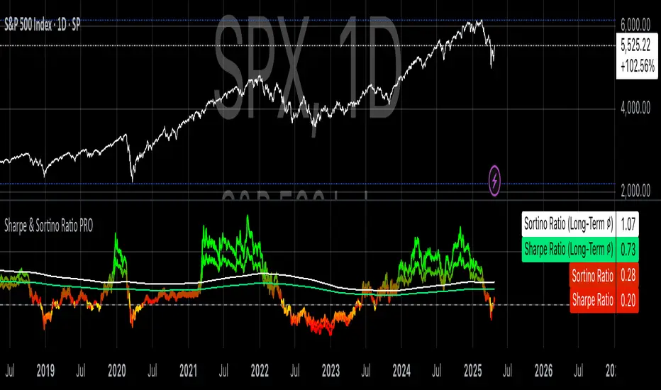
Sharpe & Sortino Ratio PROSharpe & Sortino Ratio PRO offers an advanced and more precise way to calculate and visualize the Sharpe and Sortino Ratios for financial assets on TradingView. Its main goal is to provide a scientifically accurate method for assessing the risk-adjusted performance of assets, both in the short and long term. Unlike TradingView’s built-in metrics, this script correctly handles periodic returns, uses optional logarithmic returns, properly annualizes both returns and volatility, and adjusts for the risk-free rate — all critical factors for truly meaningful Sharpe and Sortino calculations.
Users can customize the rolling analysis window (e.g., 252 periods for one year on daily data) and the long-term smoothing period (e.g., 1260 periods for five years). There’s also an option to select between linear and logarithmic returns and to manually input a risk-free rate if real-time data from FRED (the 3-Month T-Bill Rate via FRED:DGS3MO) is unavailable. Based on the chart’s timeframe (daily, weekly, or monthly), the script automatically adjusts the risk-free rate to a per-period basis.
The Sharpe Ratio is calculated by first determining the asset’s excess returns (returns after subtracting the risk-free return per period), then computing the average and standard deviation of those excess returns over the specified window, and finally annualizing these figures separately — in line with best scientific practices (Sharpe, 1994). The Sortino Ratio follows a similar approach but only considers negative returns, focusing specifically on downside risk (Sortino & Van der Meer, 1991).
To enhance readability, the script visualizes the ratios using a color gradient: strong negative values are shown in red, neutral values in yellow, and strong positive values in green. Additionally, the long-term averages for both Sharpe and Sortino are plotted with steady colors (teal and orange, respectively), making it easier to spot enduring performance trends.
Why calculating Sharpe and Sortino Ratios manually on TradingView is necessary?
While TradingView provides basic Sharpe and Sortino Ratios, they come with significant methodological flaws that can lead to misleading conclusions about an asset’s true risk-adjusted performance.
First, TradingView often computes volatility based on the standard deviation of price levels rather than returns (TradingView, 2023). This method is problematic because it causes the volatility measure to be directly dependent on the asset’s absolute price. For instance, a stock priced at $1,000 will naturally show larger absolute daily price moves than a $10 stock, even if their percentage changes are similar. This artificially inflates the measured standard deviation and, as a result, depresses the calculated Sharpe Ratio.
Second, TradingView frequently neglects to adjust for the risk-free rate. By treating all returns as risky returns, the computed Sharpe Ratio may significantly underestimate risk-adjusted performance, especially when interest rates are high (Sharpe, 1994).
Third, and perhaps most critically, TradingView doesn’t properly annualize the mean excess return and the standard deviation separately. In correct financial math, the mean excess return should be multiplied by the number of periods per year, while the standard deviation should be multiplied by the square root of the number of periods per year (Cont, 2001; Fabozzi et al., 2007). Incorrect annualization skews the Sharpe and Sortino Ratios and can lead to under- or overestimating investment risk.
These flaws lead to three major issues:
• Overstated volatility for high-priced assets.
• Incorrect scaling between returns and risk.
• Sharpe Ratios that are systematically biased downward, especially in high-price or high-interest environments.
How to properly calculate Sharpe and Sortino Ratios in Pine Script?
To get accurate results, the Sharpe and Sortino Ratios must be calculated using the correct methodology:
1. Use returns, not price levels, to calculate volatility. Ideally, use logarithmic returns for better mathematical properties like time additivity (Cont, 2001).
2. Adjust returns by subtracting the risk-free rate on a per-period basis to obtain true excess returns.
3. Annualize separately:
• Multiply the mean excess return by the number of periods per year (e.g., 252 for daily data).
• Multiply the standard deviation by the square root of the number of periods per year.
4. Finally, divide the annualized mean excess return by the annualized standard deviation to calculate the Sharpe Ratio.
The Sortino Ratio follows the same structure but uses downside deviations instead of standard deviations.
By following this scientifically sound method, you ensure that your Sharpe and Sortino Ratios truly reflect the asset’s real-world risk and return characteristics.
References
• Cont, R. (2001). Empirical properties of asset returns: stylized facts and statistical issues. Quantitative Finance, 1(2), pp. 223–236.
• Fabozzi, F.J., Gupta, F. and Markowitz, H.M. (2007). The Legacy of Modern Portfolio Theory. Journal of Investing, 16(3), pp. 7–22.
• Sharpe, W.F. (1994). The Sharpe Ratio. Journal of Portfolio Management, 21(1), pp. 49–58.
• Sortino, F.A. and Van der Meer, R. (1991). Downside Risk: Capturing What’s at Stake in Investment Situations. Journal of Portfolio Management, 17(4), pp. 27–31.
• TradingView (2023). Help Center - Understanding Sharpe and Sortino Ratios. Available at: www.tradingview.com (Accessed: 25 April 2025).
MA Crossover [AlchimistOfCrypto]🌌 MA Crossover Quantum – Illuminating Market Harmonic Patterns 🌌
Category: Trend Analysis Indicators 📈
"The moving average crossover, reinterpreted through quantum field principles, visualizes the underlying resonance structures of price movements. This indicator employs principles from molecular orbital theory where energy states transition through gradient fields, similar to how price momentum shifts between bullish and bearish phases. Our implementation features algorithmically optimized parameters derived from extensive Python-based backtesting, creating a visual representation of market energy flows with dynamic opacity gradients that highlight the catalytic moments where trend transformations occur."
📊 Professional Trading Application
The MA Crossover Quantum transcends the traditional moving average crossover with a sophisticated gradient illumination system that highlights the energy transfer between fast and slow moving averages. Scientifically optimized for multiple timeframes and featuring eight distinct visual themes, it enables traders to perceive trend transitions with unprecedented clarity.
⚙️ Indicator Configuration
- Timeframe Presets 📏
Python-optimized parameters for specific timeframes:
- 1H: EMA 23/395 - Ideal for intraday precision trading
- 4H: SMA 41/263 - Balanced for swing trading operations
- 1D: SMA 8/44 - Optimized for daily trend identification
- 1W: SMA 32/38 - Calibrated for medium-term position trading
- 2W: SMA 17/20 - Engineered for long-term investment signals
- Custom Settings 🎯
Full parameter customization available for professional traders:
- Fast/Slow MA Length: Fine-tune to specific market conditions
- MA Type: Select between EMA (exponential) and SMA (simple) calculation methods
- Visual Theming 🎨
Eight scientifically designed visual palettes optimized for neural pattern recognition:
- Neon (default): High-contrast green/red scheme enhancing trend transition visibility
- Cyan-Magenta: Vibrant palette for maximum visual distinction
- Yellow-Purple: Complementary colors for enhanced pattern recognition
- Specialized themes (Green-Red, Forest Green, Blue Ocean, Orange-Red, Grayscale): Each calibrated for different market environments
- Opacity Control 🔍
- Variable transparency system (0-100) allowing seamless integration with price action
- Adaptive glow effect that intensifies around crossover points - the "catalytic moments" of trend change
🚀 How to Use
1. Select Timeframe ⏰: Choose from scientifically optimized presets based on your trading horizon
2. Customize Parameters 🎚️: For advanced users, disable presets to fine-tune MA settings
3. Choose Visual Theme 🌈: Select a color scheme that enhances your personal pattern recognition
4. Adjust Opacity 🔎: Fine-tune visualization intensity to complement your chart analysis
5. Identify Trend Changes ✅: Monitor gradient intensity to spot high-probability transition zones
6. Trade with Precision 🛡️: Use gradient intensity variations to determine position sizing and risk management
Developed through rigorous mathematical modeling and extensive backtesting, MA Crossover Quantum transforms the fundamental moving average crossover into a sophisticated visual analysis tool that reveals the molecular structure of market momentum.

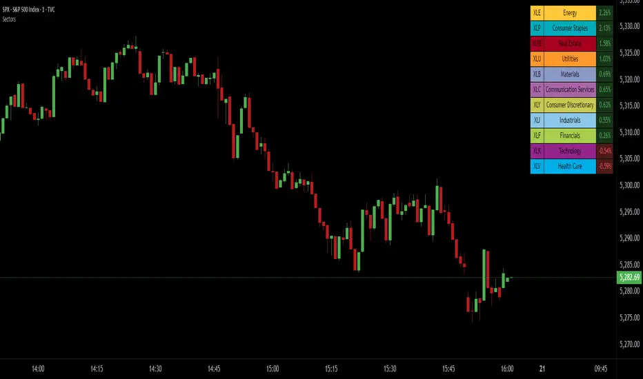
SPDR Sectors TableThis script generates an interactive and customizable SPDR Sectors Table designed to monitor and analyze the performance of the 11 main sectors of the S&P 500 via sector-specific ETFs. It offers a dynamic overview of daily or periodic sector movements, making it a valuable tool for traders, analysts, and investors implementing sector rotation strategies.
█ DEFINITIONS
SPDR Sectors ETFs are exchange-traded funds managed by State Street Global Advisors, which divide the S&P 500 into the following 11 sectors:
- Communication Services (XLC)
- Consumer Discretionary (XLY)
- Consumer Staples (XLP)
- Energy (XLE)
- Financials (XLF)
- Health Care (XLV)
- Industrials (XLI)
- Materials (XLB)
- Real Estate (XLRE)
- Technology (XLK)
- Utilities (XLU)
These ETFs aim to replicate the performance of their respective sectors as defined by the Global Industry Classification Standard (GICS). The funds are periodically rebalanced to match changes in the S&P 500 composition, offering an accurate snapshot of sectoral trends.
█ INDICATOR
The table displays each sector's ticker and full name, following official GICS terminology and SPDR color coding. It also shows percentage performance, calculated daily on intraday charts or based on the selected time frame.
Users can sort the table by either percentage performance or the relative weight of each ETF in the S&P 500. The default weight values reflect data updated as of 17 April 2025, and can be manually adjusted based on the most recent sector weightings available on the official SPDR website.
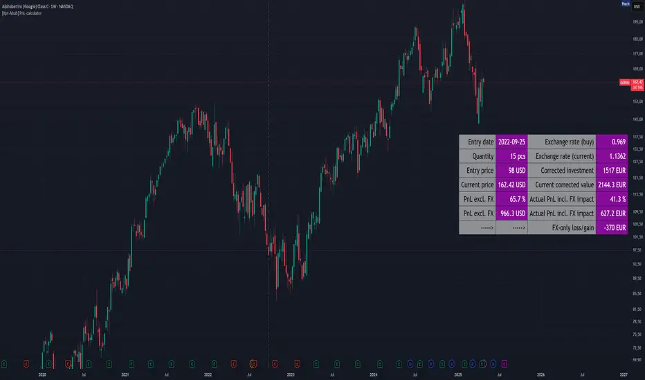
[Kpt-Ahab] PnL-calculatorThe PnL-Cal shows how much you’re up or down in your own currency, based on the current exchange rate.
Let’s say your home currency is EUR.
On October 10, 2022, you bought 10 Tesla stocks at $219 apiece.
Back then, with an exchange rate of 0.9701, you spent €2,257.40.
If you sold the 10 Tesla shares on April 17, 2025 for $241.37 each, that’s around a 10% gain in USD.
But if you converted the USD back to EUR on the same day at an exchange rate of 1.1398, you’d actually end up with an overall loss of about 6.2%.
Right now, only a single entry point is supported.
If you bought shares on different days with different exchange rates, you’ll unfortunately have to enter an average for now.
For viewing on a phone, the table can be simplified.
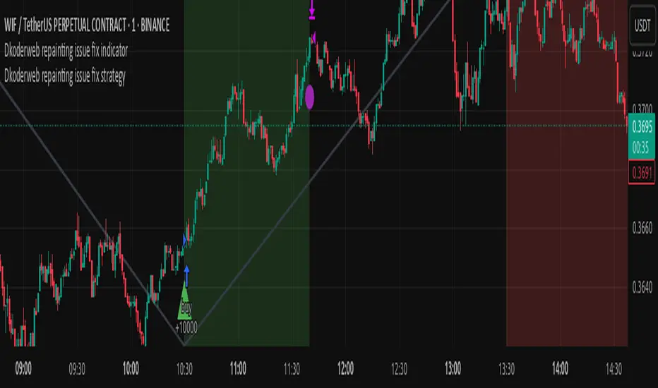
Dkoderweb repainting issue fix strategyHarmonic Pattern Recognition Trading Strategy
This TradingView strategy called "Dkoderweb repainting issue fix strategy" is designed to identify and trade harmonic price patterns with optimized entry and exit points using Fibonacci levels. The strategy implements various popular harmonic patterns including Bat, Butterfly, Gartley, Crab, Shark, ABCD, and their anti-patterns.
Key Features
Pattern Recognition: Identifies 17+ harmonic price patterns including standard and anti-patterns
Fibonacci-Based Entries and Exits: Uses customizable Fibonacci levels for precision entries, take profits, and stop losses
Alternative Timeframe Analysis: Option to use higher timeframes for pattern identification
Heiken Ashi Support: Optional use of Heiken Ashi candles instead of regular candlesticks
Visual Indicators:
Pattern visualization with ZigZag indicator
Buy/sell signal markers
Color-coded background to highlight active trade zones
Customizable Fibonacci level display
How It Works
The strategy uses a ZigZag-based pattern identification system to detect pivot points
When a valid harmonic pattern forms, the strategy calculates the optimal entry window using the specified Fibonacci level (default 0.382)
Entries trigger when price returns to the entry window after pattern completion
Take profit and stop loss levels are automatically set based on customizable Fibonacci ratios
Visual alerts notify you of entries and exits
The strategy tracks active trades and displays them with background color highlights
Customizable Settings
Trade size
Entry window Fibonacci level (default 0.382)
Take profit Fibonacci level (default 0.618)
Stop loss Fibonacci level (default -0.618)
Alert messages for entries and exits
Display options for specific Fibonacci levels
Alternative timeframe selection
This strategy is designed to fix repainting issues that are common in harmonic pattern strategies, ensuring more reliable signals and backtesting results.
Hosoda Time Cycles (Forward + Backward)Hosoda Time Cycles
Market Timing Projection Tool
The Hosoda Time Cycles indicator is inspired by the legendary Japanese trader Ichimoku Hosoda, who emphasized the power of time in forecasting market behavior. This tool visualizes forward and backward time cycles based on significant price pivots, enabling traders to anticipate potential trend shifts, consolidations, or continuations with high precision.
Key Features:
Forward & Backward Cycles: Projects future and past time intervals based on selected pivots to reveal cyclical patterns.
Manual & Auto Pivot Selection: Choose between automatic detection or manually selected swing highs/lows.
Cycle Ratios: Includes traditional Hosoda counts such as 9, 17, 26, 33, 42, and 65 — key numbers in Ichimoku time theory.
Multi-Timeframe Utility: Effective across intraday, swing, and long-term charts.
Minimalist Overlay: Clean design to avoid clutter while providing powerful cycle insights.
Customizable Visuals: Adjustable line styles, colors, and cycle projection lengths for clarity and personalization.
Ideal For:
Traders focused on time-based confluence, cycle forecasting, and market rhythm detection, especially those who blend price action with Japanese trading techniques.

Time-based Alerts for Trading Windows🌟 Time-based Alerts for Trading Windows 🌐📈
This is a re-uploaded script as the previous one got hidden.
This Time-based Alerts for Trading Windows script is a highly customizable and reliable tool designed to assist traders in managing automated strategies or manually monitoring specific market conditions. Inspired by CrossTrade's Time-based Alert, this script is tailored for those who rely on precise time windows to trigger actions, such as sending webhook signals or managing Expert Advisors (EAs).
Whether you are a scalper, day trader, or algorithmic trader, this script empowers you to stay on top of your trades with fully customizable time-based alerts.
🛠️ Customizable Time Alerts
This indicator allows you to create up to 12 unique time windows by specifying the exact hour and minute for each alert. Each time window corresponds to an individual alert condition, making it perfect for managing trades during specific market sessions or key time periods.
For example:
Alert 1 can be set at 9:30 AM (market open).
Alert 2 can be set at 3:55 PM (just before market close).
Each alert can be toggled on or off in the indicator settings, allowing you to manage alerts without having to reconfigure your script.
You can adjust the colours to fit any colour scheme you like!
🕒 Odd and Even Time Alerts
The script comes with three built-in alert type categories:
Odd Alerts (marked with a green triangle on the chart): These correspond to odd-numbered inputs like Alert 1, Alert 3, Alert 5, and so on.
Even Alerts (marked with a red triangle on the chart): These correspond to even-numbered inputs like Alert 2, Alert 4, Alert 6, and so on.
You can also customize all 12 alerts individually to include a custom alert message
These alerts serve as a convenient way to differentiate between multiple trading strategies or market conditions. You can customize alert messages for odd and even alerts directly from TradingView’s alert panel.
🔗 Webhook Integration for Automation
This script is fully compatible with webhook-based automation. By configuring your alerts in TradingView, you can send signals to trading bots, EAs, or any third-party system. For example, you can:
Turn off an EA at a specific time (e.g., 3:55 PM EST).
Send buy/sell signals to your bot during predefined trading windows.
Simply use TradingView’s alert message editor to format webhook payloads for your automation system.
🌐 Timezone Flexibility
Trading happens across multiple time zones, and this script accounts for that. You can toggle between:
Eastern Time (New York): Ideal for most US-based markets.
Central Time (Exchange): Useful for futures and commodities traders.
This ensures your alerts are always in sync with your preferred time zone, eliminating confusion.
🎨 Visual Indicators
The script plots visual markers directly on your chart to indicate active alerts:
Up Facing Triangles: Represent odd-numbered alerts, providing a quick reference for these time windows.
Down Facing Triangles: Represent even-numbered alerts, helping you track different strategies or conditions.
These visual markers make it easy to see when alerts are triggered, even at a glance.
📈 Practical Use Case
Let’s say you’re trading the USTEC index on a 1-minute chart. You want to:
Turn off your trading bot at 16:55 EST to avoid after-market volatility.
Trigger a re-entry signal at 17:30 EST to capture moves during the Asian session.
Visually monitor these actions on your chart for easy reference.
This script makes it possible with precision alerts and webhook integration. Simply configure the time windows in the settings and set up your alerts in TradingView.
🚨 How to Set Up Alerts
Enable or Disable Alerts: Use the script’s settings to toggle specific alerts on or off as needed.
Set Custom Time Windows: Define the hour and minute for each alert in the settings panel.
Create Alerts in TradingView:
Go to the TradingView alert panel.
Select the condition (e.g., "Odd Time-based Alert (Green)" or "Even Time-based Alert (Red)").
Customize the alert message for webhook integration or personal notification.
Choose the trigger type: Once Per Bar or Once Per Bar Close to keep the alert active.
Integrate with Webhooks: Use the alert message field to format payloads for automation systems like MT4, MT5, or third-party bots.
📋 Key Notes
Alerts can trigger indefinitely if set to "Once Per Bar" or "Once Per Bar Close".
Always ensure the expiration date is set far in the future to avoid unexpected alert deactivation.
Test webhook messages and alert configurations thoroughly before using them in live trading.
This script is a powerful addition to your trading toolbox, offering precision, flexibility, and automation capabilities. Whether you’re turning off an EA, managing trades during market sessions, or automating strategies via webhooks, this script is here to support you.
Start using the Time-based Alerts for Trading Windows today and trade with confidence! 🚀✨

Difference Between Candle Close and Fibonacci MA AVGIndicator calculates the first 17 Fibonacci moving averages and then finds the average. The difference between the close price and average Fibonacci MA and is then "scaled" by dividing the average Fibonacci MA.
Indicator shows the MA trend and can show possible support and resistance. Indicator shows an oscillation between an asset being overbought and oversold. Each asset has its own oscillation profile.
diff = (close - avgFibMA)/avgFibMA

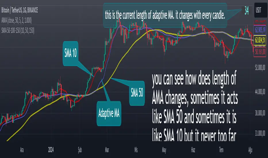
Adaptive Moving Averagewhat is the purpose of the indicator?
When short-length moving averages are used as trailing stops, they cause exiting the trade too early. Keeping the length value too high will result in exiting the transaction too late and losing most of the profits earned. I aimed to prevent this problem with this indicator.
what is "Adaptive Moving Average"?
it is a moving average that can change its length on each candle depending on the selected source.
what it does?
The indicator first finds the average lengths of the existing candles and defines different distances accordingly. When the moving average drawn by the indicator enters the area defined as "far" by the indicator, the indicator reduces the length of the moving average, preventing it from moving too far from the price, and continues to do so at different rates until the moving average gets close enough to the price. If the moving average gets close enough to the price, it starts to increase the length of the average and thus the adaptation continues.
how it does it?
Since the change of each trading pair is different in percentage terms, I chose to base the average height of the candles instead of using constant percentage values to define the concept of "far". While doing this, I used a weighted moving average so that the system could quickly adapt to the latest changes (you can see it on line 17). After calculating what percentage of the moving average this value is, I caused the length of the moving average to change in each bar depending on the multiples of this percentage value that the price moved away from the average (look at line 20, 21 and 22). Finally, I created a new moving average using this new length value I obtained.
how to use it?
Although the indicator chooses its own length, we have some inputs to customize it. First of all, we can choose which source we will use the moving average on. The "source" input allows us to use it with other indicators.
"max length" and "min length" determine the maximum and minimum value that the length of the moving average can take.
Apart from this, there are options for you to add a standard moving average to the chart so that you can compare the adaptive moving average, and bollinger band channels that you can use to create different strategies.
This indicator was developed due to the need for a more sophisticated trailing stop, but once you understand how it works, it is completely up to you to combine it with other indicators and create different strategies.
Uptrick: Volatility Reversion BandsUptrick: Volatility Reversion Bands is an indicator designed to help traders identify potential reversal points in the market by combining volatility and momentum analysis within one comprehensive framework. It calculates dynamic bands around a simple moving average and issues signals when price interacts with these bands. Below is a fully expanded description, structured in multiple sections, detailing originality, usefulness, uniqueness, and the purpose behind blending standard deviation-based and ATR-based concepts. All references to code have been removed to focus on the written explanation only.
Section 1: Overview
Uptrick: Volatility Reversion Bands centers on a moving average around which various bands are constructed. These bands respond to changes in price volatility and can help gauge potential overbought or oversold conditions. Signals occur when the price moves beyond certain thresholds, which may imply a reversal or significant momentum shift.
Section 2: Originality, Usefulness, Uniqness, Purpose
This indicator merges two distinct volatility measurements—Bollinger Bands and ATR—into one cohesive system. Bollinger Bands use standard deviation around a moving average, offering a baseline for what is statistically “normal” price movement relative to a recent mean. When price hovers near the upper band, it may indicate overbought conditions, whereas price near the lower band suggests oversold conditions. This straightforward construction often proves invaluable in moderate-volatility settings, as it pinpoints likely turning points and gauges a market’s typical trading range.
Yet Bollinger Bands alone can falter in conditions marked by abrupt volatility spikes or sudden gaps that deviate from recent norms. Intraday news, earnings releases, or macroeconomic data can alter market behavior so swiftly that standard-deviation bands do not keep pace. This is where ATR (Average True Range) adds an important layer. ATR tracks recent highs, lows, and potential gaps to produce a dynamic gauge of how much price is truly moving from bar to bar. In quieter times, ATR contracts, reflecting subdued market activity. In fast-moving markets, ATR expands, exposing heightened volatility on each new bar.
By overlaying Bollinger Bands and ATR-based calculations, the indicator achieves a broader situational awareness. Bollinger Bands excel at highlighting relative overbought or oversold areas tied to an established average. ATR simultaneously scales up or down based on real-time market swings, signaling whether conditions are calm or turbulent. When combined, this means a price that barely crosses the Bollinger Band but also triggers a high ATR-based threshold is likely experiencing a volatility surge that goes beyond typical market fluctuations. Conversely, a price breach of a Bollinger Band when ATR remains low may still warrant attention, but not necessarily the same urgency as in a high-volatility regime.
The resulting synergy offers balanced, context-rich signals. In a strong trend, the ATR layer helps confirm whether an apparent price breakout really has momentum or if it is just a temporary spike. In a range-bound market, standard deviation-based Bollinger Bands define normal price extremes, while ATR-based extensions highlight whether a breakout attempt has genuine force behind it. Traders gain clarity on when a move is both statistically unusual and accompanied by real volatility expansion, thus carrying a higher probability of a directional follow-through or eventual reversion.
Practical advantages emerge across timeframes. Scalpers in fast-paced markets appreciate how ATR-based thresholds update rapidly, revealing if a sudden price push is routine or exceptional. Swing traders can rely on both indicators to filter out false signals in stable conditions or identify truly notable moves. By calibrating to changes in volatility, the merged system adapts naturally whether the market is trending, ranging, or transitioning between these phases.
In summary, combining Bollinger Bands (for a static sense of standard-deviation-based overbought/oversold zones) with ATR (for a dynamic read on current volatility) yields an adaptive, intuitive indicator. Traders can better distinguish fleeting noise from meaningful expansions, enabling more informed entries, exits, and risk management. Instead of relying on a single yardstick for all market conditions, this fusion provides a layered perspective, encouraging traders to interpret price moves in the broader context of changing volatility.
Section 3: Why Bollinger Bands and ATR are combined
Bollinger Bands provide a static snapshot of volatility by computing a standard deviation range above and below a central average. ATR, on the other hand, adapts in real time to expansions or contractions in market volatility. When combined, these measures offset each other’s limitations: Bollinger Bands add structure (overbought and oversold references), and ATR ensures responsiveness to rapid price shifts. This synergy helps reduce noisy signals, particularly during sudden market turbulence or extended consolidations.
Section 4: User Inputs
Traders can adjust several parameters to suit their preferences and strategies. These typically include:
1. Lookback length for calculating the moving average and standard deviation.
2. Multipliers to control the width of Bollinger Bands.
3. An ATR multiplier to set the distance for additional reversal bands.
4. An option to display weaker signals when the price merely approaches but does not cross the outer bands.
Section 5: Main Calculations
At the core of this indicator are four important steps:
1. Calculate a basis using a simple moving average.
2. Derive Bollinger Bands by adding and subtracting a product of the standard deviation and a user-defined multiplier.
3. Compute ATR over the same lookback period and multiply it by the selected factor.
4. Combine ATR-based distance with the Bollinger Bands to set the outer reversal bands, which serve as stronger signal thresholds.
Section 6: Signal Generation
The script interprets meaningful reversal points when the price:
1. Crosses below the lower outer band, potentially highlighting oversold conditions where a bullish reversal may occur.
2. Crosses above the upper outer band, potentially indicating overbought conditions where a bearish reversal may develop.
Section 7: Visualization
The indicator provides visual clarity through labeled signals and color-coded references:
1. Distinct colors for upper and lower reversal bands.
2. Markers that appear above or below bars to denote possible buying or selling signals.
3. A gradient bar color scheme indicating a bar’s position between the lower and upper bands, helping traders quickly see if the price is near either extreme.
Section 8: Weak Signals (Optional)
For those preferring early cues, the script can highlight areas where the price nears the outer bands. When weak signals are enabled:
1. Bars closer to the upper reversal zone receive a subtle marker suggesting a less robust, yet still noteworthy, potential selling area.
2. Bars closer to the lower reversal zone receive a subtle marker suggesting a less robust, yet still noteworthy, potential buying area.
Section 9: Simplicity, Effectiveness, and Lower Timeframes
Although combining standard deviation and ATR involves sophisticated volatility concepts, this indicator is visually straightforward. Reversal bands and gradient-colored bars make it easy to see at a glance when price approaches or crosses a threshold. Day traders operating on lower timeframes benefit from such clarity because it helps filter out minor fluctuations and focus on more meaningful signals.
Section 10: Adaptability across Market Phases
Because both the standard deviation (for Bollinger Bands) and ATR adapt to changing volatility, the indicator naturally adjusts to various environments:
1. Trending: The additional ATR-based outer bands help distinguish between temporary pullbacks and deeper reversals.
2. Ranging: Bollinger Bands often remain narrower, identifying smaller reversals, while the outer ATR bands remain relatively close to the main bands.
Section 11: Reduced Noise in High-Volatility Scenarios
By factoring ATR into the band calculations, the script widens or narrows the thresholds during rapid market fluctuations. This reduces the amount of false triggers typically found in indicators that rely solely on fixed calculations, preventing overreactions to abrupt but short-lived price spikes.
Section 12: Incorporation with Other Technical Tools
Many traders combine this indicator with oscillators such as RSI, MACD, or Stochastic, as well as volume metrics. Overbought or oversold signals in momentum oscillators can provide additional confirmation when price reaches the outer bands, while volume spikes may reinforce the significance of a breakout or potential reversal.
Section 13: Risk Management Considerations
All trading strategies carry risk. This indicator, like any tool, can and does produce losing trades if price unexpectedly reverses again or if broader market conditions shift rapidly. Prudent traders employ protective measures:
1. Stop-loss orders or trailing stops.
2. Position sizing that accounts for market volatility.
3. Diversification across different asset classes when possible.
Section 14: Overbought and Oversold Identification
Standard Bollinger Bands highlight regions where price might be overextended relative to its recent average. The extended ATR-based reversal bands serve as secondary lines of defense, identifying moments when price truly stretches beyond typical volatility bounds.
Section 15: Parameter Customization for Different Needs
Users can tailor the script to their unique preferences:
1. Shorter lookback settings yield faster signals but risk more noise.
2. Higher multipliers spread the bands further apart, filtering out small moves but generating fewer signals.
3. Longer lookback periods smooth out market noise, often leading to more stable but less frequent trading cues.
Section 16: Examples of Different Trading Styles
1. Day Traders: Often reduce the length to capture quick price swings.
2. Swing Traders: May use moderate lengths such as 20 to 50 bars.
3. Position Traders: Might opt for significantly longer settings to detect macro-level reversals.
Section 17: Performance Limitations and Reality Check
No technical indicator is free from false signals. Sudden fundamental news events, extreme sentiment changes, or low-liquidity conditions can render signals less reliable. Backtesting and forward-testing remain essential steps to gauge whether the indicator aligns well with a trader’s timeframe, risk tolerance, and instrument of choice.
Section 18: Merging Volatility and Momentum
A critical uniqueness of this indicator lies in how it merges Bollinger Bands (standard deviation-based) with ATR (pure volatility measure). Bollinger Bands provide a relative measure of price extremes, while ATR dynamically reacts to market expansions and contractions. Together, they offer an enhanced perspective on potential market turns, ideally reducing random noise and highlighting moments where price has traveled beyond typical bounds.
Section 19: Purpose of this Merger
The fundamental purpose behind blending standard deviation measures with real-time volatility data is to accommodate different market behaviors. Static standard deviation alone can underreact or overreact in abnormally volatile conditions. ATR alone lacks a baseline reference to normality. By merging them, the indicator aims to provide:
1. A versatile dynamic range for both typical and extreme moves.
2. A filter against frequent whipsaws, especially in choppy environments.
3. A visual framework that novices and experts can interpret rapidly.
Section 20: Summary and Practical Tips
Uptrick: Volatility Reversion Bands offers a powerful tool for traders looking to combine volatility-based signals with momentum-derived reversals. It emphasizes clarity through color-coded bars, defined reversal zones, and optional weak signal markers. While potentially useful across all major timeframes, it demands ongoing risk management, realistic expectations, and careful study of how signals behave under different market conditions. No indicator serves as a crystal ball, so integrating this script into an overall strategy—possibly alongside volume data, fundamentals, or momentum oscillators—often yields the best results.
Disclaimer and Educational Use
This script is intended for educational and informational purposes. It does not constitute financial advice, nor does it guarantee trading success. Sudden economic events, low-liquidity times, and unexpected market behaviors can all undermine technical signals. Traders should use proper testing procedures (backtesting and forward-testing) and maintain disciplined risk management measures.

Ichimoku ACE ClubA. Overview:
This script is a custom implementation of the Ichimoku Cloud indicator for the TradingView platform, built using Pine Script version 4. It adds additional features like custom "Knife" lines and circle markers for specific data points. The indicator overlays on the chart and plots various elements of the Ichimoku system, including the Tenkan, Kijun, Chikou, and Kumo Cloud.
B. Inputs:
1. Tenkan (TS): This is the short-term moving average line (default period: 9).
2. Kijun (KJ): This is the medium-term moving average line (default period: 17).
3. Knife1 (K1): This line is based on a longer-term moving average (default period: 65).
4. Knife2 (K2): Another long-term moving average line (default period: 129).
5. Chikou Displacement (Chikou_Disp): The Chikou Span is plotted with a delay of 26 periods by default.
6. Displacement (disp): Determines the horizontal shift of the Kumo cloud.
C. Functions:
- `donchian(len)`: This function calculates the Donchian channel, which is the average of the highest high and the lowest low over the given period (len).
- `mf(len, offset)`: This function calculates the highest high and the lowest low over the given period, with an offset applied.
D. Plots:
1. Tenkan, Kijun, Knife1, and Knife2: These are plotted as lines with different colors and thicknesses.
- Tenkan is blue.
- Kijun is red.
- Knife1 is yellow.
- Knife2 is orange.
2. Chikou Span: This is plotted with a displacement and shown in purple.
3. Kumo Cloud: The cloud is formed by plotting two lines, Span A (green) and Span B (magenta), which represent the top and bottom of the cloud, respectively. The space between these lines is filled with a semi-transparent color, either green or magenta, depending on the relative position of the two spans.
E. Circle Markers:
- Additional circle markers are plotted for each of the Tenkan, Kijun, Knife1, and Knife2 lines at various offsets, helping to visualize the historical data points for each of these indicators. These circles are color-coded according to the line they correspond to.
F. Customization:
- The indicator allows customization of the lengths (periods) for Tenkan, Kijun, Knife1, Knife2, and other components via the script's input fields.
G. Conclusion:
This Ichimoku-based indicator provides a detailed view of the market's trend strength and direction. It offers a unique addition with the Knife lines and visual aids like circle markers for specific periods, which helps traders make better-informed decisions based on Ichimoku analysis.
---
You can modify the parameters such as `TS`, `KJ`, `K1`, `K2`, and `disp` according to your trading preferences. The colors and line thicknesses can also be adjusted for better visual representation.

BKLevelsThis displays levels from a text input, levels from certain times on the previous day, and high/low/close from previous day. The levels are drawn for the date in the first line of the text input. Newlines are required between each level
Example text input:
2024-12-17
SPY,606,5,1,Lower Hvol Range,FIRM
SPY,611,1,1,Last 20K CBlock,FIRM
SPY,600,2,1,Last 20K PBlock,FIRM
SPX,6085,1,1,HvolC,FIRM
SPX,6080,2,1,HvolP,FIRM
SPX,6095,3,1,Upper PDVR,FIRM
SPX,6060,3,1,Lower PDVR,FIRM
For each line, the format is ,,,,,
For color, there are 9 possible user- configurable colors- so you can input numbers 1 through 9
For line style, the possible inputs are:
"FIRM" -> solid line
"SHORT_DASH" -> dotted line
"MEDIUM_DASH" -> dashed line
"LONG_DASH" -> dashed line
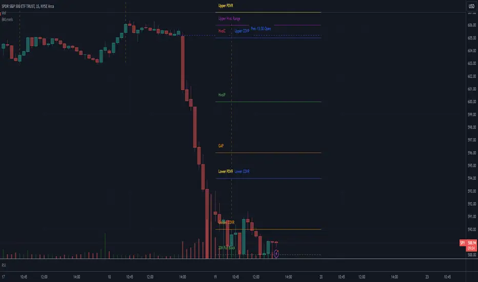
ATT + Key Levels with SessionsKey Features:
ATT Turning Point Numbers:
This input allows the user to define specific numbers (e.g., "3,11,17,29,41,47,53,59") that mark turning points in price action, which are checked using the bar_index modulo 60. If the current bar index matches one of these turning points, it triggers potential buy or sell signals.
RSI (Relative Strength Index):
The RSI is calculated based on a user-defined period (rsi_period), typically 14, and used to indicate overbought or oversold conditions. The script defines overbought (70) and oversold (30) levels, which are used to filter buy or sell signals.
Session Times:
The script includes predefined session times for major trading markets:
New York: From 9:30 AM EST to 4:00 PM EST.
London: From 8:00 AM GMT to 4:30 PM GMT.
Asia: From 12:00 AM GMT to 9:00 AM GMT.
These session times are used to restrict the buy and sell signals to specific market sessions.
Key Levels:
The script calculates and plots key market levels for the current day and week:
Daily High and Low: The highest and lowest prices of the current day.
Weekly High and Low: The highest and lowest prices of the current week.
These levels are plotted with different colors for visual reference.
Signal Logic:
Buy Signal: Triggered when the current bar is a turning point (according to the ATT model), the RSI is below the oversold threshold, and the current time is within the active session times (New York, London, or Asia).
Sell Signal: Triggered when the current bar is a turning point, the RSI is above the overbought threshold, and the current time is within the active session times.
Signal Limitations:
A user-defined limit (max_signals_per_session) controls the maximum number of signals that can be plotted within each session. This prevents excessive signal generation.
Plotting and Background Highlights:
Buy and Sell Signals: The script plots shapes (labels) above or below the bars to indicate buy or sell signals when the conditions are met.
Background Highlight: The background color is highlighted in yellow when the current bar matches one of the defined ATT turning points.
In Summary:
The indicator combines multiple technical factors to generate trading signals:
Turning points in price action (based on custom ATT numbers),
RSI levels (overbought/oversold),
Market session times (New York, London, Asia),
Key price levels (daily and weekly highs and lows).
This combination helps traders identify potential buying and selling opportunities while considering broader market dynamics and limiting the number of signals during each session.

Ensemble Alerts█ OVERVIEW
This indicator creates highly customizable alert conditions and messages by combining several technical conditions into groups , which users can specify directly from the "Settings/Inputs" tab. It offers a flexible framework for building and testing complex alert conditions without requiring code modifications for each adjustment.
█ CONCEPTS
Ensemble analysis
Ensemble analysis is a form of data analysis that combines several "weaker" models to produce a potentially more robust model. In a trading context, one of the most prevalent forms of ensemble analysis is the aggregation (grouping) of several indicators to derive market insights and reinforce trading decisions. With this analysis, traders typically inspect multiple indicators, signaling trade actions when specific conditions or groups of conditions align.
Simplifying ensemble creation
Combining indicators into one or more ensembles can be challenging, especially for users without programming knowledge. It usually involves writing custom scripts to aggregate the indicators and trigger trading alerts based on the confluence of specific conditions. Making such scripts customizable via inputs poses an additional challenge, as it often involves complicated input menus and conditional logic.
This indicator addresses these challenges by providing a simple, flexible input menu where users can easily define alert criteria by listing groups of conditions from various technical indicators in simple text boxes . With this script, you can create complex alert conditions intuitively from the "Settings/Inputs" tab without ever writing or modifying a single line of code. This framework makes advanced alert setups more accessible to non-coders. Additionally, it can help Pine programmers save time and effort when testing various condition combinations.
█ FEATURES
Configurable alert direction
The "Direction" dropdown at the top of the "Settings/Inputs" tab specifies the allowed direction for the alert conditions. There are four possible options:
• Up only : The indicator only evaluates upward conditions.
• Down only : The indicator only evaluates downward conditions.
• Up and down (default): The indicator evaluates upward and downward conditions, creating alert triggers for both.
• Alternating : The indicator prevents alert triggers for consecutive conditions in the same direction. An upward condition must be the first occurrence after a downward condition to trigger an alert, and vice versa for downward conditions.
Flexible condition groups
This script features six text inputs where users can define distinct condition groups (ensembles) for their alerts. An alert trigger occurs if all the conditions in at least one group occur.
Each input accepts a comma-separated list of numbers with optional spaces (e.g., "1, 4, 8"). Each listed number, from 1 to 35, corresponds to a specific individual condition. Below are the conditions that the numbers represent:
1 — RSI above/below threshold
2 — RSI below/above threshold
3 — Stoch above/below threshold
4 — Stoch below/above threshold
5 — Stoch K over/under D
6 — Stoch K under/over D
7 — AO above/below threshold
8 — AO below/above threshold
9 — AO rising/falling
10 — AO falling/rising
11 — Supertrend up/down
12 — Supertrend down/up
13 — Close above/below MA
14 — Close below/above MA
15 — Close above/below open
16 — Close below/above open
17 — Close increase/decrease
18 — Close decrease/increase
19 — Close near Donchian top/bottom (Close > (Mid + HH) / 2)
20 — Close near Donchian bottom/top (Close < (Mid + LL) / 2)
21 — New Donchian high/low
22 — New Donchian low/high
23 — Rising volume
24 — Falling volume
25 — Volume above average (Volume > SMA(Volume, 20))
26 — Volume below average (Volume < SMA(Volume, 20))
27 — High body to range ratio (Abs(Close - Open) / (High - Low) > 0.5)
28 — Low body to range ratio (Abs(Close - Open) / (High - Low) < 0.5)
29 — High relative volatility (ATR(7) > ATR(40))
30 — Low relative volatility (ATR(7) < ATR(40))
31 — External condition 1
32 — External condition 2
33 — External condition 3
34 — External condition 4
35 — External condition 5
These constituent conditions fall into three distinct categories:
• Directional pairs : The numbers 1-22 correspond to pairs of opposing upward and downward conditions. For example, if one of the inputs includes "1" in the comma-separated list, that group uses the "RSI above/below threshold" condition pair. In this case, the RSI must be above a high threshold for the group to trigger an upward alert, and the RSI must be below a defined low threshold to trigger a downward alert.
• Non-directional filters : The numbers 23-30 correspond to conditions that do not represent directional information. These conditions act as filters for both upward and downward alerts. Traders often use non-directional conditions to refine trending or mean reversion signals. For instance, if one of the input lists includes "30", that group uses the "Low relative volatility" condition. The group can trigger an upward or downward alert only if the 7-period Average True Range (ATR) is below the 40-period ATR.
• External conditions : The numbers 31-35 correspond to external conditions based on the plots from other indicators on the chart. To set these conditions, use the source inputs in the "External conditions" section near the bottom of the "Settings/Inputs" tab. The external value can represent an upward, downward, or non-directional condition based on the following logic:
▫ Any value above 0 represents an upward condition.
▫ Any value below 0 represents a downward condition.
▫ If the checkbox next to the source input is selected, the condition becomes non-directional . Any group that uses the condition can trigger upward or downward alerts only if the source value is not 0.
To learn more about using plotted values from other indicators, see this article in our Help Center and the Source input section of our Pine Script™ User Manual.
Group markers
Each comma-separated list represents a distinct group , where all the listed conditions must occur to trigger an alert. This script assigns preset markers (names) to each condition group to make the active ensembles easily identifiable in the generated alert messages and labels. The markers assigned to each group use the format "M", where "M" is short for "Marker" and "x" is the group number. The titles of the inputs at the top of the "Settings/Inputs" tab show these markers for convenience.
For upward conditions, the labels and alert messages show group markers with upward triangles (e.g., "M1▲"). For downward conditions, they show markers with downward triangles (e.g., "M1▼").
NOTE: By default, this script populates the "M1" field with a pre-configured list for a mean reversion group ("2,18,24,28"). The other fields are empty. If any "M*" input does not contain a value, the indicator ignores it in the alert calculations.
Custom alert messages
By default, the indicator's alert message text contains the activated markers and their direction as a comma-separated list. Users can override this message for upward or downward alerts with the two text fields at the bottom of the "Settings/Inputs" tab. When the fields are not empty , the alerts use that text instead of the default marker list.
NOTE: This script generates alert triggers, not the alerts themselves. To set up an alert based on this script's conditions, open the "Create Alert" dialog box, then select the "Ensemble Alerts" and "Any alert() function call" options in the "Condition" tabs. See the Alerts FAQ in our Pine Script™ User Manual for more information.
Condition visualization
This script offers organized visualizations of its conditions, allowing users to inspect the behaviors of each condition alongside the specified groups. The key visual features include:
1) Conditional plots
• The indicator plots the history of each individual condition, excluding the external conditions, as circles at different levels. Opposite conditions appear at positive and negative levels with the same absolute value. The plots for each condition show values only on the bars where they occur.
• Each condition's plot is color-coded based on its type. Aqua and orange plots represent opposing directional conditions, and purple plots represent non-directional conditions. The titles of the plots also contain the condition numbers to which they apply.
• The plots in the separate pane can be turned on or off with the "Show plots in pane" checkbox near the top of the "Settings/Inputs" tab. This input only toggles the color-coded circles, which reduces the graphical load. If you deactivate these visuals, you can still inspect each condition from the script's status line and the Data Window.
• As a bonus, the indicator includes "Up alert" and "Down alert" plots in the Data Window, representing the combined upward and downward ensemble alert conditions. These plots are also usable in additional indicator-on-indicator calculations.
2) Dynamic labels
• The indicator draws a label on the main chart pane displaying the activated group markers (e.g., "M1▲") each time an alert condition occurs.
• The labels for upward alerts appear below chart bars. The labels for downward alerts appear above the bars.
NOTE: This indicator can display up to 500 labels because that is the maximum allowed for a single Pine script.
3) Background highlighting
• The indicator can highlight the main chart's background on bars where upward or downward condition groups activate. Use the "Highlight background" inputs in the "Settings/Inputs" tab to enable these highlights and customize their colors.
• Unlike the dynamic labels, these background highlights are available for all chart bars, irrespective of the number of condition occurrences.
█ NOTES
• This script uses Pine Script™ v6, the latest version of TradingView's programming language. See the Release notes and Migration guide to learn what's new in v6 and how to convert your scripts to this version.
• This script imports our new Alerts library, which features functions that provide high-level simplicity for working with complex compound conditions and alerts. We used the library's `compoundAlertMessage()` function in this indicator. It evaluates items from "bool" arrays in groups specified by an array of strings containing comma-separated index lists , returning a tuple of "string" values containing the marker of each activated group.
• The script imports the latest version of the ta library to calculate several technical indicators not included in the built-in `ta.*` namespace, including Double Exponential Moving Average (DEMA), Triple Exponential Moving Average (TEMA), Fractal Adaptive Moving Average (FRAMA), Tilson T3, Awesome Oscillator (AO), Full Stochastic (%K and %D), SuperTrend, and Donchian Channels.
• The script uses the `force_overlay` parameter in the label.new() and bgcolor() calls to display the drawings and background colors in the main chart pane.
• The plots and hlines use the available `display.*` constants to determine whether the visuals appear in the separate pane.
Look first. Then leap.

Forward Price Performance TableThis calculates the percentage price changes for three key timeframes:
1 week (5 trading days ago)
1 month (17 trading days ago),
3 months (45 trading days ago).
This is to show a forward looking performance based on earlier timeframes that traditionally used. This is the framework I team uses to calculate performance metrics.

ATT Model with Buy/Sell SignalsIndicator Summary
This indicator is based on the ATT (Arithmetic Time Theory) model, using specific turning points derived from the ATT sequence (3, 11, 17, 29, 41, 47, 53, 59) to identify potential market reversals. It also integrates the RSI (Relative Strength Index) to confirm overbought and oversold conditions, triggering buy and sell signals when conditions align with the ATT sequence and RSI level.
Turning Points: Detected based on the ATT sequence applied to bar count. This suggests high-probability areas where the market could turn.
RSI Filter: Adds strength to the signals by ensuring buy signals occur when RSI is oversold (<30) and sell signals when RSI is overbought (>70).
Max Signals Per Session: Limits signals to two per session to reduce over-trading.
Entry Criteria
Buy Signal: Enter a buy trade if:
The indicator displays a green "BUY" marker.
RSI is below the oversold level (default <30), suggesting a potential upward reversal.
Sell Signal: Enter a sell trade if:
The indicator displays a red "SELL" marker.
RSI is above the overbought level (default >70), indicating a potential downward reversal.
Exit Criteria
Take Profit (TP):
Define TP as a fixed percentage or point value based on the asset's volatility. For example, set TP at 1.5-2x the risk, or a predefined point target (like 50-100 points).
Alternatively, exit the position when price approaches a key support/resistance level or the next significant swing high/low.
Stop Loss (SL):
Place the SL below the recent low (for buys) or above the recent high (for sells).
Set a fixed SL in points or percentage based on the asset’s average movement range, like an ATR-based stop, or limit it to a specific risk amount per trade (1-2% of account).
Trailing into Profit
Use a trailing strategy to lock in profits and let winning trades run further. Two main options:
ATR Trailing Stop:
Set the trailing stop based on the ATR (Average True Range), adjusting every time a new candle closes. This can help in volatile markets by keeping the stop at a consistent distance based on recent price movement.
Break-Even and Partial Profits:
When the price moves in your favor by a set amount (e.g., 1:1 risk/reward), move SL to the entry (break-even).
Take partial profit at intermediate levels (e.g., 50% at 1:1 RR) and trail the remainder.
Risk Management for Prop Firm Evaluation
Prop firms often have strict rules on daily loss limits, max drawdowns, and minimum profit targets. Here’s how to align your strategy with these:
Limit Risk per Trade:
Keep risk per trade to a conservative level (e.g., 1% or lower of your account balance). This allows for more room in case of a drawdown and aligns with most prop firm requirements.
Daily Loss Limits:
Set a daily stop-loss that ensures you don’t exceed the firm’s rules. For example, if the daily limit is 5%, stop trading once you reach a 3-4% drawdown.
Avoid Over-Trading:
Stick to the max signals per session rule (one or two trades). Taking only high-probability setups reduces emotional and reactive trades, preserving capital.
Stick to a Profit Target:
Aim to meet the evaluation’s profit goal efficiently but avoid risky or oversized trades to reach it faster.
Avoid Major Economic Events:
News events can disrupt technical setups. Avoid trading around significant releases (like FOMC or NFP) to reduce the chance of sudden losses due to high volatility.
Summary
Using this strategy with discipline, a structured entry/exit approach, and tight risk management can maximize your chances of passing a prop firm evaluation. The ATT model’s turning points, combined with the RSI, provide an edge by highlighting reversal zones, while limiting trades to 1-2 per session helps maintain controlled risk.

Pulse DPO: Major Cycle Tops and Bottoms█ OVERVIEW
Pulse DPO is an oscillator designed to highlight Major Cycle Tops and Bottoms .
It works on any market driven by cycles. It operates by removing the short-term noise from the price action and focuses on the market's cyclical nature.
This indicator uses a Normalized version of the Detrended Price Oscillator (DPO) on a 0-100 scale, making it easier to identify major tops and bottoms.
Credit: The DPO was first developed by William Blau in 1991.
█ HOW TO READ IT
Pulse DPO oscillates in the range between 0 and 100. A value in the upper section signals an OverBought (OB) condition, while a value in the lower section signals an OverSold (OS) condition.
Generally, the triggering of OB and OS conditions don't necessarily translate into swing tops and bottoms, but rather suggest caution on approaching a market that might be overextended.
Nevertheless, this indicator has been customized to trigger the signal only during remarkable top and bottom events.
I suggest using it on the Daily Time Frame , but you're free to experiment with this indicator on other time frames.
The indicator has Built-in Alerts to signal the crossing of the Thresholds. Please don't act on an isolated signal, but rather integrate it to work in conjunction with the indicators present in your Trading Plan.
█ OB SIGNAL ON: ENTERING OVERBOUGHT CONDITION
When Pulse DPO crosses Above the Top Threshold it Triggers ON the OB signal. At this point the oscillator line shifts to OB color.
When Pulse DPO enters the OB Zone, please beware! In this Area the Major Players usually become Active Sellers to the Public. While the OB signal is On, it might be wise to Consider Selling a portion or the whole Long Position.
Please note that even though this indicator aims to focus on major tops and bottoms, a strong trending market might trigger the OB signal and stay with it for a long time. That's especially true on young markets and on bubble-mode markets.
█ OB SIGNAL OFF: EXITING OVERBOUGHT CONDITION
When Pulse DPO crosses Below the Top Threshold it Triggers OFF the OB signal. At this point the oscillator line shifts to its normal color.
When Pulse DPO exits the OB Zone, please beware because a Major Top might just have occurred. In this Area the Major Players usually become Aggressive Sellers. They might wind up any remaining Long Positions and Open new Short Positions.
This might be a good area to Open Shorts or to Close/Reverse any remaining Long Position. Whatever you choose to do, it's usually best to act quickly because the market is prone to enter into panic mode.
█ OS SIGNAL ON: ENTERING OVERSOLD CONDITION
When Pulse DPO crosses Below the Bottom Threshold it Triggers ON the OS signal. At this point the oscillator line shifts to OS color.
When Pulse DPO enters the OS Zone, please beware because in this Area the Major Players usually become Active Buyers accumulating Long Positions from the desperate Public.
While the OS signal is On, it might be wise to Consider becoming a Buyer or to implement a Dollar-Cost Averaging (DCA) Strategy to build a Long Position towards the next Cycle. In contrast to the tops, the OS state usually takes longer to resolve a major bottom.
█ OS SIGNAL OFF: EXITING OVERSOLD CONDITION
When Pulse DPO crosses Above the Bottom Threshold it Triggers OFF the OS signal. At this point the oscillator line shifts to its normal color.
When Pulse DPO exits the OS Zone, please beware because a Major Bottom might already be in place. In this Area the Major Players become Aggresive Buyers. They might wind up any remaining Short Positions and Open new Long Positions.
This might be a good area to Open Longs or to Close/Reverse any remaining Short Positions.
█ WHY WOULD YOU BE INTERESTED IN THIS INDICATOR?
This indicator is built over a solid foundation capable of signaling Major Cycle Tops and Bottoms across many markets. Let's see some examples:
Early Bitcoin Years: From 0 to 1242
This chart is in logarithmic mode in order to properly display various exponential cycles. Pulse DPO is properly signaling the major early highs from 9-Jun-2011 at 31.50, to the next one on 9-Apr-2013 at 240 and the epic top from 29-Nov-2013 at 1242.
Due to the massive price movements, the OB condition stays pinned during most of the exponential price action. But as you can see, the OB condition quickly vanishes once the Cycle Top has been reached. As the market matures, the OB condition becomes more exceptional and triggers much closer from the Cycle Top.
With regards to Cycle Bottoms, the early bottom of 2 after having peaked at 31.50 doesn’t get captured by the indicator. That is the only cycle bottom that escapes the Pulse DPO when the bottom threshold is set at a value of 5. In that event, the oscillator low reached 6.95.
Bitcoin Adoption Spreading: From 257 to 73k
This chart is in logarithmic mode in order to properly display various exponential cycles. Pulse DPO is properly signaling all the major highs from 17-Dec-2017 at 19k, to the next one on 14-Apr-2021 at 64k and the most recent top from 9-Nov-2021 at 68k.
During the massive run of 2017, the OB condition still stayed triggered for a few weeks on each swing top. But on the next cycles it started to signal only for a few days before each swing top actually happened. The OB condition during the last cycle top triggered only for 3 days. Therefore the signal grows in focus as the market matures.
At the time of publishing this indicator, Bitcoin printed a new All Time High (ATH) on 13-Mar-2024 at 73k. That run didn’t trigger the OB condition. Therefore, if the indicator is correct the Bitcoin market still has some way to grow during the next months.
With regards to Cycle Bottoms, the bottom of 3k after having peaked at19k got captured within the wide OS zone. The bottom of 15k after having peaked at 68k got captured too within the OS accumulation area.
Gold
Pulse DPO behaves surprisingly well on a long standing market such as Gold. Moving back to the 197x years it’s been signaling most Cycle Tops and Bottoms with precision. During the last cycle, it shows topping at 2k and bottoming at 1.6k.
The current price action is signaling OB condition in the range of 2.5k to 2.7k. Looking at past cycles, it tends to trigger on and off at multiple swing tops until reaching the final cycle top. Therefore this might indicate the first wave within a potential gold run.
Oil
On the Oil market, we can see that most of the cycle tops and bottoms since the 80s got signaled. The only exception being the low from 2020 which didn’t trigger.
EURUSD
On Forex markets the Pulse DPO also behaves as expected. Looking back at EURUSD we can see the marketing triggering OB and OS conditions during major cycle tops and bottoms from recent times until the 80s.
S&P 500
On the S&P 500 the Pulse DPO catched the lows from 2016 and 2020. Looking at present price action, the recent ATH didn’t trigger the OB condition. Therefore, the indicator is allowing room for another leg up during the next months.
Amazon
On the Amazon chart the Pulse DPO is mirroring pretty accurately the major swings. Scrolling back to the early 2000s, this chart resembles early exponential swings in the crypto space.
Tesla
Moving onto a younger tech stock, Pulse DPO captures pretty accurately the major tops and bottoms. The chart is shown in logarithmic scale to better display the magnitude of the moves.
█ SETTINGS
This indicator is ideal for identifying major market turning points while filtering out short-term noise. You are free to adjust the parameters to align with your preferred trading style.
Parameters : This section allows you to customize any of the Parameters that shape the Oscillator.
Oscillator Length: Defines the period for calculating the Oscillator.
Offset: Shifts the oscillator calculation by a certain number of periods, which is typically half the Oscillator Length.
Lookback Period: Specifies how many bars to look back to find tops and bottoms for normalization.
Smoothing Length: Determines the length of the moving average used to smooth the oscillator.
Thresholds : This section allows you to customize the Thresholds that trigger the OB and OS conditions.
Top: Defines the value of the Top Threshold.
Bottom: Defines the value of the Bottom Threshold.

Flashtrader´s Statistical BandwidthsThe vast majority of traders exclusively concern
themselves with trend-following in all its facets. Scoring
points with trends on a regular basis is a difficult task
since prices do not constantly move in one direction
or another. In the case of the DAX future, for example,
only about 30 per cent of all trading days in a year are
trend days. And of these, there are x percent long ones
and x per cent short ones. Catching the very days when
prices rise or fall from the opening to the close is a major
challenge for a trader who also needs to have previously
recognised the corresponding direction.
However, there are also other ways of profit-taking
every day – for example, by using the mean reversion
strategy. The idea behind this is the fact that prices reach
a high and a low every day – but very rarely close at the
high or the low. This means that prices always move
away from these extreme points and the closing price is
somewhere in between. A profitable trading strategy can
be developed out of this.
But how can you know where the high and the low
will be tomorrow? Is it possible for you to know this in
advance? No – because no one can predict the future. Or
can they? At least it can be statistically determined how
high or low prices could go tomorrow. There is a high
degree of probability that one of the two possibilities
will materialise. It will then be necessary to act.
Calculation
Classic pivot points for the following day are calculated
from the high, low and closing price. But does it really
make sense to use such a mix? I don’t think so and
use a different calculation for this strategy. In a first step,
only the differences between the start and the high or low
are calculated on a daily basis. To avoid being dependent
on individual days and outliers, it is advisable to calculate,
in a second step, the average of these differences over
the past five days. Finally, this average will then be added
at the opening price of the current trading day for the
upper statistical bandwidth and subtracted for the lower
bandwidth.
upper bandwidth = oSTB (violet dashed line in the chart)
lower bandwidth = uSTB (violet dashedline in the chart)
The second interesting question is, if the previous day's high has been exceeded, how much further can the price rise from a mathematical/statistical point of view?
These calculated previous day highs expansions are shown as red dashed lines
Previous day's high expansion = VTHA
Previous day's low expansion = VTTA
For further orientation, the previous day's high (VTH) and the previous day's low (VTT) are shown in light blue dashed lines
And as a supplement, the previous day's close in the DAX Future at 10:00 p.m. VTSA in violet solid lines and the previous day's close in the cash register at 5:30 p.m. VTSN in yellow solid lines
Reaching the calculated extreme values does not mean that the trend has to change immediately, but there is at least temporary exhaustion potential with which you can earn a few points every day in the area of scalping.
Example for cheap entry long:
Example for cheap entry short:
Deutsch:
Die Masse der Trader beschäftigt sich ausschließlich mit Trendfolge in all ihren Facetten. Mit Trends regelmäßig zu punkten ist ein schwieriges Unterfangen, da die Kurse nicht ständig in die eine oder andere Richtung laufen. Beim DAX-Future zum Beispiel sind von allen Börsentagen im Jahr lediglich zirka 30 Prozent Trendtage. Davon sind dann auch noch x Prozent Long und x Prozent Short. Hier genau die Tage abzupassen, an denen die Kurse von Börsenbeginn bis zum Schluss steigen beziehungsweise fallen, ist eine große Herausforderung – wobei der Trader zuvor noch die entsprechende Richtung erkannt haben muss. Es gibt jedoch auch noch andere Methoden täglich Gewinne mitzunehmen, zum Beispiel mit der Mean-Reversion-Strategie (Mittelwertumkehr).
Hintergrund ist die Tatsache, dass die Kurse jeden Tag ein Hoch und ein Tief erreichen – aber sehr selten am Hoch oder am Tief schließen. Das bedeutet, dass die Preise sich immer wie der von diesen Extrempunkten wegbewegen und der Schlusskurs irgendwo dazwischen liegt. Hieraus lässt sich eine profitable Handelsstrategie entwickeln. Aber woher kannst Du wissen, wo morgen das Hoch und das Tief sein wird? Kannst Du das vorher schon wissen? Nein – denn niemand kann die Zukunft vorhersagen. Oder doch? Statistisch lässt sich zumindest bestimmen, wie hoch und wie tief die Kurse morgen steigen oder fallen könnten. Eine Seite wird mit sehr hoher Wahrscheinlichkeit ein treffen. Dann gilt es zu handeln.
Berechnung Klassischer Pivot-Punkte für den folgenden Tag werden aus Hoch, Tief und Schlusskurs berechnet. Aber ist es wirklich sinnvoll, einen solchen Mix zu verwenden? Ich finde das nicht und verwenden für diese Strategie eine andere Berechnung. Im ersten Schritt werden täglich die Differenzen nur vom Start bis zum Hoch beziehungsweise Tief errechnet. Um nicht von einzelnen Tagen und Ausreißern abhängig zu sein, empfiehlt es sich, in einem zweiten Schritt den Durchschnitt dieser Differenzen über die letzten fünf Tage zu errechnen. Zuletzt wird dann dieser Durchschnitt zum Eröffnungskurs des aktuellen Handelstages für die obere statistische Bandbreite addiert und für die untere Bandbreite subtrahiert.
Obere statistische Bandbreite = oSTB (violette gestrichelte Linie im Chart)
Untere statistische Bandbreite = uSTB (violette gestrichelte Linie im Chart)
Die zweite interessante Frage ist, wenn das Vortageshoch überschritten wurde, wie weit kann der Kurs dann noch steigen aus mathematisch/statistischer Sicht?
Diese berechneten Vortagesextremausdehnungen sind als rote gestrichelte Linien dargestellt
Vortageshochausdehnung = VTHA
Vortagestiefausdehnung = VTTA
Für die weitere Orientierung sind die Vortageshochs (VTH) und die Vortagestiefs (VTT) als hellblaue gestrichelte Linien abgebildet.
Als Ergänzung wird noch der Vortages Schluss im Dax Future um 22:00 Uhr VTSA mit einer violetten durchgezogenen Linie und der Kassamarktschluss um 17:30 Uhr mit einer gelben durchgezogenen Linie gezeigt.
Das Erreichen der berechneten Extremwerte bedeutet nicht, das der Trend sofort drehen muss, aber es sind zumindest temporäre Erschöpfungspotentiale mit denen sich im Bereich scalping täglich einige Punkte verdienen lassen.
Beispiel für günstigen Einstieg Long:
Beispiel für günstigen Einstieg Short:
