[2020 Updated]Bitcoin Logarithmic Growth CurvesCredit goes to the original writer of the script, Quantadelic, who generously allowed anyone to copy/edit. I adjusted the value of the bottom/top intercept and slope to better fit the March 2020 coronavirus dip.
Use Bitstamp BTCUSD for better reading.
Cari dalam skrip untuk "2020年3月+中证芯片产业指数+成分股调整"

2020 March 27 .BXBT IndexAs described here:
www.bitmex.com
blog.bitmex.com
With itBit's weight given to \Gemini because it currently is not on TradingView and they're both small NY based exchanges.
BITSTAMP: 24.86%
BITTREX: 2.53%
COINBASE: 44.98%
GEMINI: 7.41%
KRAKEN: 20.22%
BITSTAMP:BTCUSD^0.2486*BITTREX:BTCUSD^0.0253*COINBASE:BTCUSD^0.4498*GEMINI:BTCUSD^0.0741*KRAKEN:XBTUSD^0.2022
Intended for use with volume based indicators because BitMEX's indices do not include volume data.

Summer 2020/2021The Pine Script indicator you are examining is designed to enhance your trading chart by visually demarcating specific seasonal periods known as summer for the years 2020 and 2021. This indicator achieves this by employing background shading to indicate these defined summer periods, providing traders with a visual reference to help in analyzing seasonal trends and making informed decisions.
The script operates with precision by defining two critical summer periods: one for the year 2020 and another for the year 2021. The summer period, in this context, is identified as the time span between June 21 and September 22 of each specified year. The script utilizes the Pine Script timestamp function to create exact date and time boundaries for these periods, marking June 21 as the start of summer and September 22 as the end of summer for each year.
In detail, the indicator sets up two distinct background colors to represent the summer periods of 2020 and 2021. Specifically, it employs a semi-transparent blue color to signify the summer period of 2020, and a semi-transparent green color to denote the summer period of 2021. This differentiation in colors allows for easy visual distinction between the two years on the chart.
To achieve this visual effect, the script continuously evaluates the current bar's timestamp against the defined summer periods. If the current bar falls within the summer range of 2020, the background is shaded with the specified blue hue. Conversely, if the current bar is within the summer range of 2021, the background is shaded with the green hue. This approach ensures that the chart background reflects the specific summer periods accurately and distinctly.
By incorporating this indicator into your TradingView chart, you gain the ability to visually distinguish between different summer periods of consecutive years. This can be particularly useful for analyzing how market behavior or price movements vary during these specific times, facilitating better trend analysis and decision-making based on historical seasonal patterns.
Overall, this indicator serves as a practical tool for enhancing your chart's clarity and providing a seasonal context that can aid in the evaluation of trading strategies and historical market trends during the summer months of 2020 and 2021.

Velocity To Inverse Correlation to VIX/Bonds Strategy (2020)This strategy measures and creates a signal when an asset is moving out of a correlation with high yield bonds or the CBOE VIX into an inverse correlation, as well as when an asset is losing correlation with a top corporate bonds ETF. When this signal is triggered, the simulation has the portfolio asset go long.
Additionally, exits are based on a 2% stop loss and a 2% take profit for simplicity sake to indicate whether the direct next move in the asset is up or down.
This was originally tested as a descent indicator for Ethereum's 2020 moves as institutional investors moved into the market.

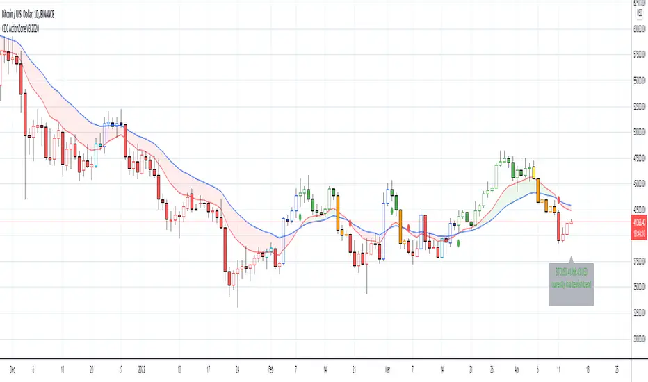
CDC ActionZone V3 2020## CDC ActionZone V3 2020 ##
This is an update to my earlier script, CDC ActionZone V2
The two scripts works slightly differently with V3 reacting slightly faster.
The main update is focused around conforming the standard to Pine Script V4.
## How it works ##
ActionZone is a very simple system, utilizing just two exponential moving
averages. The 'Zones' in which different 'actions' should be taken is
highlighted with different colors on the chart. Calculations for the zones
are based on the relative position of price to the two EMA lines and the
relationship between the two EMAs
CDCActionZone is your barebones basic, tried and true, trend following system
that is very simple to follow and has also proven to be relatively safe.
## How to use ##
The basic method for using ActionZone is to follow the green/red color.
Buy when bar closes in green.
Sell when bar closes in red.
There is a small label to help with reading the buy and sell signal.
Using it this way is safe but slow and is expected to have around 35-40%
accuracy, while yielding around 2-3 profit factors. The system works best
on larger time frames.
The more advanced method uses the zones to switch between different
trading system and biases, or in conjunction with other indicators.
example 1:
Buy when blue and Bullish Divergence between price and RSI is visible,
if not Buy on Green and vise-versa
example 2:
Set up a long-biased grid and trade long only when actionzone is in
green, yellow or orange.
change the bias to short when actionzone turns to te bearish side
(red, blue, aqua)
(Look at colors on a larger time frame)
## Note ##
The price field is set to close by default. change to either HL2 or OHLC4
when using the system in intraday timeframes or on market that does not close
(ie. Cryptocurrencies)
## Note2 ##
The fixed timeframe mode is for looking at the current signal on a larger time frame
ie. When looking at charts on 1h you can turn on fixed time frame on 1D to see the
current 'zone' on the daily chart plotted on to the hourly chart.
This is useful if you wanted to use the system's 'Zones' in conjunction with other
types of signals like Stochastic RSI, for example.
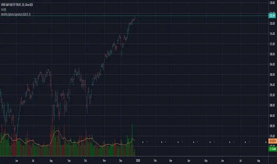
Monthly Options Expiration 2020Monthly options expiration for the year 2020.
Also you can set a flag X no. of days before the expiration date. I use it at as marker to take off existing positions in expiration week or roll to next expiration date or to place new trades.
Happy new year 2020 and all the best traders.
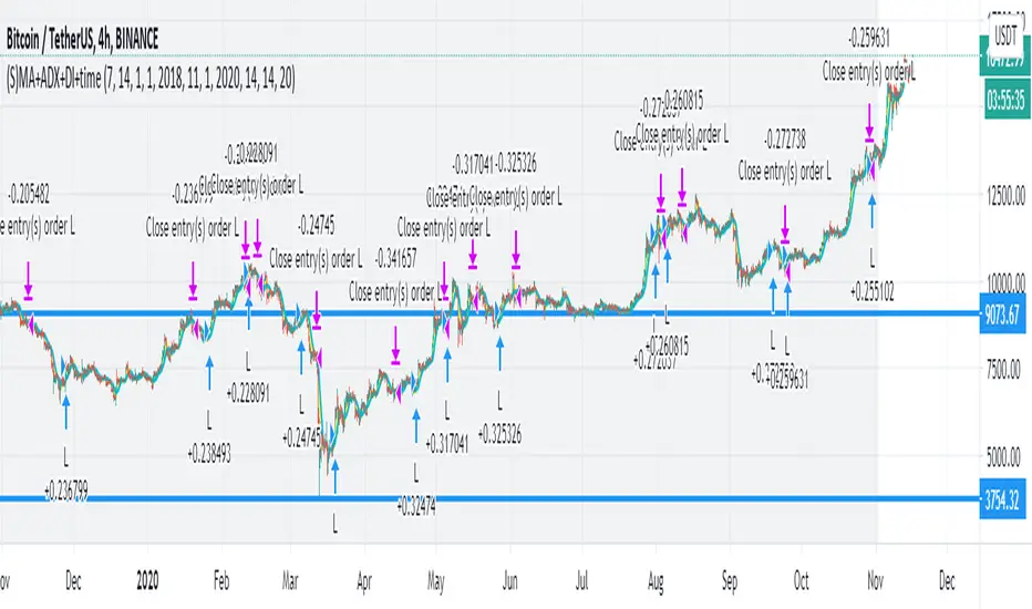
BTC and ETH Long strategy - version 2I wrote my first article in May 2020. See below
BTC and ETH Long strategy - version1
After 6 months, it is now time to check the result of my script for the last 6 months.
XBTUSD (4H): 14/05/2020 --> 22/11/2020 = +78% in 4 trades
ETHXBT (4H): 14/05/2020 --> 22/11/2020 = +21% in 9 trades
ETHUSD (4H): 14/05/2020 --> 22/11/2020 = +90% in 6 trades
Using the signals from this strategy to trade manually has shown that this was a bit frustrating because of the low rate of winning trades.
If you have to enter 100 trades and see 75% of them failing and 25% winning, this is frustrating. For sure the strategy makes good money but it is difficult to hold this mentality.
So, I have reviewed and modified it to get a higher winning rate.
After few days of work, tests and validation, I managed to get a wining rate close to 60%.
The key element was also to decrease the number of trades by using a higher time frame. (4H candles instead of 2H candles).
- Entry in position is based on
MACD, EMA (20), SMA (100), SMA (200) moving up
AND EMA (20) > SMA (100)
AND SMA (100) > SMA (200)
- Exit the position if: Stoploss is reached OR EMA (20) crossUnder SMA (100)
The goal of this new script is to be able to follow the signals manually and only make few trades per years.
I have also validated it against some other altcoins where some are giving very good results.
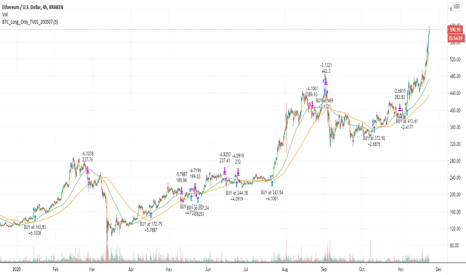
Here are some results for 2020 (from 01/01/2020 until now (22/11/2020). Those results are the one I get when using 4H candles.
ETH/USD: +144% in 8 trades.
BTC/USD: +120% in 7 trades.
ETH/BTC: +33% in 9 trades.
ICX/USD: +123% in 10 trades.
LINK/USD: +155% in 11 trades.
MLN/USD: +388% in 8 trades.
ADA/USD: +180% in 7 trades.
LINK/BTC: +97% in 10 trades.
The best is that above results are without considering compound effect. If you re-invest all gains done in each new trade, this will give you the below results :)
ETH/USD: +189% in 8 trades.
BTC/USD: +260% in 7 trades.
ETH/BTC: +29% in 9 trades.
ICX/USD: +112% in 10 trades.
LINK/USD: +222% in 11 trades.
MLN/USD: +793% in 8 trades.
ADA/USD: +319% in 7 trades.
LINK/BTC: +103% in 10 trades.
As you can see, the results are good and the number of trades for 11 months is not big, which allows the trader to place orders manually.
But still, I'm lazy :), so, I have also coded this strategy in HaasScript language which allows you to automate this strategy using the HaasOnline software specialized in automated crypto trading.
I hope that this strategy will give you ideas or will be the starting point for your own strategy.
Let me know if you need more details.
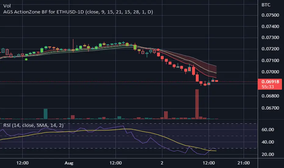
CDC ActionZone BF for ETHUSD-1D © PRoSkYNeT-EE
Based on improvements from "Kitti-Playbook Action Zone V.4.2.0.3 for Stock Market"
Based on improvements from "CDC Action Zone V3 2020 by piriya33"
Based on Triple MACD crossover between 9/15, 21/28, 15/28 for filter error signal (noise) from CDC ActionZone V3
MACDs generated from the execution of millions of times in the "Brute Force Algorithm" to backtest data from the past 5 years. ( 2017-08-21 to 2022-08-01 )
Released 2022-08-01
***** The indicator is used in the ETHUSD 1 Day period ONLY *****
Recommended Stop Loss : -4 % (execute stop Loss after candlestick has been closed)
Backtest Result ( Start $100 )
Winrate 63 % (Win:12, Loss:7, Total:19)
Live Days 1,806 days
B : Buy
S : Sell
SL : Stop Loss
2022-07-19 07 - 1,542 : B 6.971 ETH
2022-04-13 07 - 3,118 : S 8.98 % $10,750 12,7,19 63 %
2022-03-20 07 - 2,861 : B 3.448 ETH
2021-12-03 07 - 4,216 : SL -8.94 % $9,864 11,7,18 61 %
2021-11-30 07 - 4,630 : B 2.340 ETH
2021-11-18 07 - 3,997 : S 13.71 % $10,832 11,6,17 65 %
2021-10-05 07 - 3,515 : B 2.710 ETH
2021-09-20 07 - 2,977 : S 29.38 % $9,526 10,6,16 63 %
2021-07-28 07 - 2,301 : B 3.200 ETH
2021-05-20 07 - 2,769 : S 50.49 % $7,363 9,6,15 60 %
2021-03-30 07 - 1,840 : B 2.659 ETH
2021-03-22 07 - 1,681 : SL -8.29 % $4,893 8,6,14 57 %
2021-03-08 07 - 1,833 : B 2.911 ETH
2021-02-26 07 - 1,445 : S 279.27 % $5,335 8,5,13 62 %
2020-10-13 07 - 381 : B 3.692 ETH
2020-09-05 07 - 335 : S 38.43 % $1,407 7,5,12 58 %
2020-07-06 07 - 242 : B 4.199 ETH
2020-06-27 07 - 221 : S 28.49 % $1,016 6,5,11 55 %
2020-04-16 07 - 172 : B 4.598 ETH
2020-02-29 07 - 217 : S 47.62 % $791 5,5,10 50 %
2020-01-12 07 - 147 : B 3.644 ETH
2019-11-18 07 - 178 : S -2.73 % $536 4,5,9 44 %
2019-11-01 07 - 183 : B 3.010 ETH
2019-09-23 07 - 201 : SL -4.29 % $551 4,4,8 50 %
2019-09-18 07 - 210 : B 2.740 ETH
2019-07-12 07 - 275 : S 63.69 % $575 4,3,7 57 %
2019-05-03 07 - 168 : B 2.093 ETH
2019-04-28 07 - 158 : S 29.51 % $352 3,3,6 50 %
2019-02-15 07 - 122 : B 2.225 ETH
2019-01-10 07 - 125 : SL -6.02 % $271 2,3,5 40 %
2018-12-29 07 - 133 : B 2.172 ETH
2018-05-22 07 - 641 : S 5.95 % $289 2,2,4 50 %
2018-04-21 07 - 605 : B 0.451 ETH
2018-02-02 07 - 922 : S 197.42 % $273 1,2,3 33 %
2017-11-11 07 - 310 : B 0.296 ETH
2017-10-09 07 - 297 : SL -4.50 % $92 0,2,2 0 %
2017-10-07 07 - 311 : B 0.309 ETH
2017-08-22 07 - 310 : SL -4.02 % $96 0,1,1 0 %
2017-08-21 07 - 323 : B 0.310 ETH
The Lazy Trader - Index (ETF) Trend Following Robot50/150 moving average, index (ETF) trend following robot. Coded for people who cannot psychologically handle dollar-cost-averaging through bear markets and extreme drawdowns (although DCA can produce better results eventually), this robot helps you to avoid bear markets. Be a fair-weathered friend of Mr Market, and only take up his offer when the sun is shining! Designed for the lazy trader who really doesn't care...
Recommended Chart Settings:
Asset Class: ETF
Time Frame: Daily
Necessary ETF Macro Conditions:
a) Country must have healthy demographics, good ratio of young > old
b) Country population must be increasing
c) Country must be experiencing price-inflation
Default Robot Settings:
Slow Moving Average: 50 (integer) //adjust to suit your underlying index
Fast Moving Average: 150 (integer) //adjust to suit your underlying index
Bullish Slope Angle: 5 (degrees) //up angle of moving averages
Bearish Slope Angle: -5 (degrees) //down angle of moving averages
Average True Range: 14 (integer) //input for slope-angle formula
Risk: 100 (%) //100% risk means using all equity per trade
ETF Test Results (Default Settings):
SPY (1993 to 2020, 27 years), 332% profit, 20 trades, 6.4 profit factor, 7% drawdown
EWG (1996 to 2020, 24 years), 310% profit, 18 trades, 3.7 profit factor, 10% drawdown
EWH (1996 to 2020, 24 years), 4% loss, 26 trades, 0.9 profit factor, 36% drawdown
QQQ (1999 to 2020, 21 years), 232% profit, 17 trades, 3.6 profit factor, 2% drawdown
EEM (2003 to 2020, 17 years), 73% profit, 17 trades, 1.1 profit factor, 3% drawdown
GXC (2007 to 2020, 13 years), 18% profit, 14 trades, 1.3 profit factor, 26% drawdown
BKF (2009 to 2020, 11 years), 11% profit, 13 trades, 1.2 profit factor, 33% drawdown
A longer time in the markets is better, with the exception of EWH. 6 out of 7 tested ETFs were profitable, feel free to test on your favourite ETF (default settings) and comment below.
Risk Warning:
Not tested on commodities nor other financial products like currencies (code will not work), feel free to leave comments below.
Moving Average Slope Angle Formula:
Reproduced and modified from source:

BTC and ETH Long strategy - version 1I will start with a small introduction about myself. I'm now trading cryto currencies manually for almost 2 years. I decided to start after watching a documentary on the TV showing people who made big money during the Bitcoin pump which happened at the end of 2017.
The next day, I asked myself "Why should I not give it a try and learn how to trade".
This was in February 2018 and the price of Bitcoin was around 11500USD.
I didn't know how to trade. In fact, I didn't know the trading industry at all.
So, my first step into trading was to open an account with a broken. Then I directly bought 200$ worst of BTC . At that time, I saw the graph and thought "This can only go back in the upward direction!" :)
I didn't know anything about Stop loss, Take profit and Risk management.
Today, almost 2 years after, I think that I know how to trade and can also confirm that I still hold this bag of 200$ of bitcoin from 2018 :)
I did spend the 2 last years to learn technical analysis , risk management and leverage trading.
Today (14/05/2020), I know what I'm doing and I'm happy to see that the 2 last years have been positive in terms of gains. Of course, I did not make crazy money with my saving but at least I made more than if I would have kept it in my bank account.
Even if I like trading, I have a full time job which requires my full energy and lots of focus, so, the biggest problem I had is that I didn't have enough time to look at the charts.
Also, I realized that sometimes, neither technical analysis , nor fundamentals worked with crypto currency (at least for short time trading). So, as I have a developer background I decided to try to have a look at algo trading.
The goal for me was neither to make complex algos nor to beat the market but just to automate my trading with simple bot catching the big waves.
I then started to take a look at TV pine script and played with it.
I did my first LONG script in February 2020 to Long the BTC Market. It has some limitations but works well enough for me for the time being. Even if the real trades will bring me half of what the back testing shows, this will still be a lot more than what I was used to win during the last 2 years with my manual trading.
So, here we are! Below you will find some details about my first LONG script. I'm happy to share it with you.
Feel free to play with it, give your comments and bring improvements to it.
But please note that it only works fine with the candle size and crypto pair that I have mentioned below. If you use other settings this algo might loose money!
- Crypto pairs : XBTUSD and ETHXBT
- Candle size: 2 Hours
- Indicator used: Volatility , MACD (12, 26, 7), SMA (100), SMA (200), EMA (20)
- Default StopLoss: -1.5%
- Entry in position if: Volatility < 2%
AND MACD moving up
AND AME (20) moving up
AND SMA (100) moving up
AND SMA (200) moving up
AND EMA (20) > SAM (100)
AND SMA (100) > SMA (200)
- Exit the postion if: Stoploss is reached
OR EMA (20) crossUnder SMA (100)
Here is a summary of the results for this script:
XBTUSD : 01/01/2019 --> 14/05/2020 = +107%
ETHXBT : 01/01/2019 --> 14/05/2020 = +39%
ETHUSD : 01/01/2019 --> 14/05/2020 = +112%
It is far away from being perfect. There are still plenty of things which can be done to improve it but I just wanted to share it :) .
Enjoy playing with it....

Ichimoku Kinkō hyō Keizen 改MTF善The script is not finnished yet and show's an other interpretation of how it could be scripted
Step -1 is complete... Basic Ichimoku with asjutable length and editable lines colors and visibilities.
Step -2 in progress... Adding ability to une multiple Spans, sens and Kumo on higher and lower timeframe.
Your Step : Like and Share ;) have a good year 2020 !
2020-01-06 /--------/ -R.V.
Jan 06
Release Notes: The script is not finnished yet and show's an other interpretation of how it could be scripted
Step -1 is complete... Basic Ichimoku with asjutable length and editable lines colors and visibilities.
Step -2 in progress... Adding ability to une multiple Spans, sens and Kumo on higher and lower timeframe.
Your Step : Like and Share ;) have a good year 2020 !
2020-01-06 /--------/ -R.V.
Jan 07
Jan 13
Release Notes: MTF Ichimoku is on it's way !!
Jan 17
Release Notes: The script is not finnished yet and show's an interpretation of how it could be scripted
Step -1 is complete... Basic Ichimoku with asjutable length and editable lines colors and visibilities.
Step -2 in complete... Adding ability to use multiple Spans, sens and Kumo on higher timeframe.
Step -3 in progress... Creating a UNIX based function to framgments actual chart periods in subcandles or "Subprices/periods" to plot multiple Spans, sens and Kumo on LOWER timeframe.
Your Step : Like and Share ;) have a good year 2020 !
/--------Coder--------/ -R.V.

JPMorgan G7 Volatility IndexThe JPMorgan G7 Volatility Index: Scientific Analysis and Professional Applications
Introduction
The JPMorgan G7 Volatility Index (G7VOL) represents a sophisticated metric for monitoring currency market volatility across major developed economies. This indicator functions as an approximation of JPMorgan's proprietary volatility indices, providing traders and investors with a normalized measurement of cross-currency volatility conditions (Clark, 2019).
Theoretical Foundation
Currency volatility is fundamentally defined as "the statistical measure of the dispersion of returns for a given security or market index" (Hull, 2018, p.127). In the context of G7 currencies, this volatility measurement becomes particularly significant due to the economic importance of these nations, which collectively represent more than 50% of global nominal GDP (IMF, 2022).
According to Menkhoff et al. (2012, p.685), "currency volatility serves as a global risk factor that affects expected returns across different asset classes." This finding underscores the importance of monitoring G7 currency volatility as a proxy for global financial conditions.
Methodology
The G7VOL indicator employs a multi-step calculation process:
Individual volatility calculation for seven major currency pairs using standard deviation normalized by price (Lo, 2002)
- Weighted-average combination of these volatilities to form a composite index
- Normalization against historical bands to create a standardized scale
- Visual representation through dynamic coloring that reflects current market conditions
The mathematical foundation follows the volatility calculation methodology proposed by Bollerslev et al. (2018):
Volatility = σ(returns) / price × 100
Where σ represents standard deviation calculated over a specified timeframe, typically 20 periods as recommended by the Bank for International Settlements (BIS, 2020).
Professional Applications
Professional traders and institutional investors employ the G7VOL indicator in several key ways:
1. Risk Management Signaling
According to research by Adrian and Brunnermeier (2016), elevated currency volatility often precedes broader market stress. When the G7VOL breaches its high volatility threshold (typically 1.5 times the 100-period average), portfolio managers frequently reduce risk exposure across asset classes. As noted by Borio (2019, p.17), "currency volatility spikes have historically preceded equity market corrections by 2-7 trading days."
2. Counter-Cyclical Investment Strategy
Low G7 volatility periods (readings below the lower band) tend to coincide with what Shin (2017) describes as "risk-on" environments. Professional investors often use these signals to increase allocations to higher-beta assets and emerging markets. Campbell et al. (2021) found that G7 volatility in the lowest quintile historically preceded emerging market outperformance by an average of 3.7% over subsequent quarters.
3. Regime Identification
The normalized volatility framework enables identification of distinct market regimes:
- Readings above 1.0: Crisis/high volatility regime
- Readings between -0.5 and 0.5: Normal volatility regime
- Readings below -1.0: Unusually calm markets
According to Rey (2015), these regimes have significant implications for global monetary policy transmission mechanisms and cross-border capital flows.
Interpretation and Trading Applications
G7 currency volatility serves as a barometer for global financial conditions due to these currencies' centrality in international trade and reserve status. As noted by Gagnon and Ihrig (2021, p.423), "G7 currency volatility captures both trade-related uncertainty and broader financial market risk appetites."
Professional traders apply this indicator in multiple contexts:
- Leading indicator: Research from the Federal Reserve Board (Powell, 2020) suggests G7 volatility often leads VIX movements by 1-3 days, providing advance warning of broader market volatility.
- Correlation shifts: During periods of elevated G7 volatility, cross-asset correlations typically increase what Brunnermeier and Pedersen (2009) term "correlation breakdown during stress periods." This phenomenon informs portfolio diversification strategies.
- Carry trade timing: Currency carry strategies perform best during low volatility regimes as documented by Lustig et al. (2011). The G7VOL indicator provides objective thresholds for initiating or exiting such positions.
References
Adrian, T. and Brunnermeier, M.K. (2016) 'CoVaR', American Economic Review, 106(7), pp.1705-1741.
Bank for International Settlements (2020) Monitoring Volatility in Foreign Exchange Markets. BIS Quarterly Review, December 2020.
Bollerslev, T., Patton, A.J. and Quaedvlieg, R. (2018) 'Modeling and forecasting (un)reliable realized volatilities', Journal of Econometrics, 204(1), pp.112-130.
Borio, C. (2019) 'Monetary policy in the grip of a pincer movement', BIS Working Papers, No. 706.
Brunnermeier, M.K. and Pedersen, L.H. (2009) 'Market liquidity and funding liquidity', Review of Financial Studies, 22(6), pp.2201-2238.
Campbell, J.Y., Sunderam, A. and Viceira, L.M. (2021) 'Inflation Bets or Deflation Hedges? The Changing Risks of Nominal Bonds', Critical Finance Review, 10(2), pp.303-336.
Clark, J. (2019) 'Currency Volatility and Macro Fundamentals', JPMorgan Global FX Research Quarterly, Fall 2019.
Gagnon, J.E. and Ihrig, J. (2021) 'What drives foreign exchange markets?', International Finance, 24(3), pp.414-428.
Hull, J.C. (2018) Options, Futures, and Other Derivatives. 10th edn. London: Pearson.
International Monetary Fund (2022) World Economic Outlook Database. Washington, DC: IMF.
Lo, A.W. (2002) 'The statistics of Sharpe ratios', Financial Analysts Journal, 58(4), pp.36-52.
Lustig, H., Roussanov, N. and Verdelhan, A. (2011) 'Common risk factors in currency markets', Review of Financial Studies, 24(11), pp.3731-3777.
Menkhoff, L., Sarno, L., Schmeling, M. and Schrimpf, A. (2012) 'Carry trades and global foreign exchange volatility', Journal of Finance, 67(2), pp.681-718.
Powell, J. (2020) Monetary Policy and Price Stability. Speech at Jackson Hole Economic Symposium, August 27, 2020.
Rey, H. (2015) 'Dilemma not trilemma: The global financial cycle and monetary policy independence', NBER Working Paper No. 21162.
Shin, H.S. (2017) 'The bank/capital markets nexus goes global', Bank for International Settlements Speech, January 15, 2017.

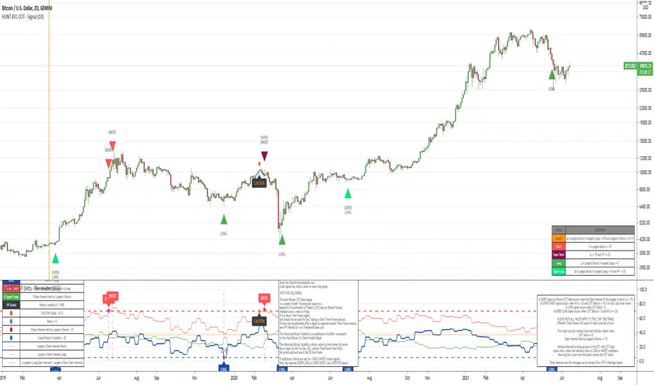
The Insider - Hunt Bitcoin CoT DeltaThe Insider - Hunt Bitcoin CoT Delta
The gift of the Squeeze in the Largest 4 open Interest Shorts vs Longs.
Why Bother another CoT signal?
Its different & focused on the Insider's.
Performance -
This Indicator provided a
1. Signal 1 = 26th March 2019 = SUPER LONG at $4,500 that saw a near $14,000 run up
2. Signal 2 = 18th & 24th June 2019 = SHORT at the second & final level $11,700 after repeated attempts & failure in the $13K range, the mini Echo Bitcoin Bull of 2019
3. Signal 3 = 17th December 2019 = LONG $6,900, Bitcoin rallied to Mid $10,500's
4. Signal 4 = 18th Feb 2020 = SUPER SHORT from $9,700's to a final extreme Low of $3,000, calling the CV-19 collapse
5. Signal 5 = 17th March 2020 = LONG from $5,400 no closure point yet
6. Signal 6 = 29th June 2020 = SUPER LONG reiterate from $10,700 no closure sell signal yet
7. Signal 7 = 17th May 2020 = LONG another accumulate LONG with no sell signal yet generated at Post H&S's low of $33,000
Note - This indicator only commences March 2019, as Bitcoin futures were a recent introduction and needed to settle for 6 months in both use and data, no signals were meaningful prior & data was light.
What is Provided. - Please note the need to also add the Hunt Bitcoin Historical Volatility Indicator for full understanding.
We provide 3 things with the 3 indicators.
'Insider' indications from Largest players in the futures market.
1. Bitcoin Macro Buy Signals.
a) The Bitcoin Commitment of Traders results see us focus solely on Largest 4 Short Open Interest & Largest 4 Long Open Interest aspects of the CoT Release data.
When the difference - is tight, a kind of pinch, these have been great Buy signals in Bitcoin.
We call this difference the Delta & When Delta is 5% or less Bitcoin is a Buy.
2. Bitcoin Macro Sells.
a) A sell signal is Triggered in Bitcoin at any point the Largest 4 short OI > or = to 70
3. AMPLIFIER Trade signals 'Super' Longs or Shorts -
Extreme low volatility events leads to highly impulsive & volatile subsequent moves, if either of 1 or 2 above occur, combined with extreme low volatility
a 'Super Long' or 'SUPER SELL' is generated. In the case of the short side, given Bitcoins general expansive and MACRO Bull trend since inception, we seek an additional component
that is an extreme differential/Delta reading between 4 biggest Longs & Shorts OI.
Namely CoT Delta also must be > 47.5%
We also have a Cautionary level, where it is not necessarily a good idea to accumulate Bitcon, as a better opportunity lower may avail itself, see conditions below.
So the required logic explicitly stated below for all Signals.
1. Long - Hunt Bitcoin CoT Delta < or = 5
2. SUPER Long - Hunt Bitcoin CoT Delta < or = 5; and 2 Day Historical Bitcoin Volatility = or < 20
3. Short - Largest 4 Sellers OI = or > 70
4. SUPER Short - Largest 4 Sellers OI = or > 70; AND..
Hunt Bitcoin CoT Delta = or > 47.5 AND 2 Day Historical BTC Volatility = or < 20
5. Caution - Largest 4 Sellers OI = or > 67.5 AND Hunt Bitcoin CoT Delta = or > 45
WARNING SEE Notes Below
Note 1 - = Largest 4 Open Interest Shorts
Note 2 - = Largest 4 Open Interest Longs
Note 3 - = Hunt Cot Delta = (Largest 4 sellers OI) -( Largest 4 Buyers OI)
Caution = Avoid new Bitcoin Accumulation Right Now, A sell signal might follow Enter on next Long
Note 4 - The Hunt Bitcoin COT Delta signal is a Largest 'Insider' Tracking tool based on a segment of Commitment of Traders data on Bitcoin Futures, released once a week on a Friday.
It is a Macro Timeframe signal , and should not be used for Day trading and Short Timeframe analysis , Entries may be optimised after a Hunt Bitcoin CoT Signal is generated by separate shorter Timeframe analysis.
Note 5 - The Historical Bitcoin Volatility is an additional 'Amplifier' component to the 'Hunt Bitcoin Cot Delta' Insider Signal
Note 6 - The Historical Bitcoin Volatility criteria varies by timeframe, the above levels are those applying on a Two Day TF Chart, select this custom timeframe in Trading View.
if additional criteria are met for LONG & SHORT insider signals, they may become 'Super Longs/Shorts', see conditions box above.
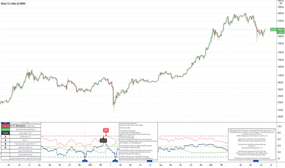
The Signal - Hunt Bitcoin CoT Buy/SellThe Signal - Hunt Bitcoin CoT Buy/Sell
Why Bother with another CoT signal?
Its different & focused on the Insider's. The Largest 4 Open Interest Seller and the Largest 4 open Interest Longs, plus the distance they are apart, the Delta, what does high percentage of Largest 4 sellers mean with a low 4 OI Buyers. , what when the usually higher Sellers are low and the largest 4 buyers almost the same value , Time to track the insiders Delta..
Performance -
This Indicator provided a
1. Signal 1 = 26th March 2019 = SUPER LONG at $4,500 that saw a near $14,000 run up
2. Signal 2 = 18th & 24th June 2019 = SHORT at the second & final level $11,700 after repeated attempts & failure in the $13K range, the mini Echo Bitcoin Bull of 2019
3. Signal 3 = 17th December 2019 = LONG $6,900, Bitcoin rallied to Mid $10,500's
4. Signal 4 = 18th Feb 2020 = SUPER SHORT from $9,700's to a final extreme Low of $3,000, calling the CV-19 collapse
5. Signal 5 = 17th March 2020 = LONG from $5,400 no closure point yet
6. Signal 6 = 29th June 2020 = SUPER LONG reiterate from $10,700 no closure sell signal yet
7. Signal 7 = 17th May 2020 = LONG another accumulate LONG with no sell signal yet generated at Post H&S's low of $33,000
Note - This indicator only commences March 2019, as Bitcoin futures were a recent introduction and needed to settle for 6 months in both use and data, no signals were meaningful prior & data was light.
What is Provided. - Please note the need to also add the Hunt Bitcoin Historical Volatility Indicator for full understanding.
We provide 3 things with the 3 indicators.
'Insider' indications from Largest players in the futures market.
1. Bitcoin Macro Buy Signals.
a) The Bitcoin Commitment of Traders results see us focus solely on Largest 4 Short Open Interest & Largest 4 Long Open Interest aspects of the CoT Release data.
When the difference - is tight, a kind of pinch, these have been great Buy signals in Bitcoin.
We call this difference the Delta & When Delta is 5% or less Bitcoin is a Buy.
2. Bitcoin Macro Sells.
a) A sell signal is Triggered in Bitcoin at any point the Largest 4 short OI > or = to 70
3. AMPLIFIER Trade signals 'Super' Longs or Shorts -
Extreme low volatility events leads to highly impulsive & volatile subsequent moves, if either of 1 or 2 above occur, combined with extreme low volatility
a 'Super Long' or 'SUPER SELL' is generated. In the case of the short side, given Bitcoins general expansive and MACRO Bull trend since inception, we seek an additional component
that is an extreme differential/Delta reading between 4 biggest Longs & Shorts OI.
Namely CoT Delta also must be > 47.5%
We also have a Cautionary level, where it is not necessarily a good idea to accumulate Bitcon, as a better opportunity lower may avail itself, see conditions below.
So the required logic explicitly stated below for all Signals.
1. Long - Hunt Bitcoin CoT Delta < or = 5
2. SUPER Long - Hunt Bitcoin CoT Delta < or = 5; and 2 Day Historical Bitcoin Volatility = or < 20
3. Short - Largest 4 Sellers OI = or > 70
4. SUPER Short - Largest 4 Sellers OI = or > 70; AND..
Hunt Bitcoin CoT Delta = or > 47.5 AND 2 Day Historical BTC Volatility = or < 20
5. Caution - Largest 4 Sellers OI = or > 67.5 AND Hunt Bitcoin CoT Delta = or > 45
WARNING SEE Notes Below
Note 1 - = Largest 4 Open Interest Shorts
Note 2 - = Largest 4 Open Interest Longs
Note 3 - = Hunt Cot Delta = (Largest 4 sellers OI) -( Largest 4 Buyers OI)
Caution = Avoid new Bitcoin Accumulation Right Now, A sell signal might follow Enter on next Long
Note 4 - The Hunt Bitcoin COT Delta signal is a Largest 'Insider' Tracking tool based on a segment of Commitment of Traders data on Bitcoin Futures, released once a week on a Friday.
It is a Macro Timeframe signal , and should not be used for Day trading and Short Timeframe analysis , Entries may be optimised after a Hunt Bitcoin CoT Signal is generated by separate shorter Timeframe analysis.
Note 5 - The Historical Bitcoin Volatility is an additional 'Amplifier' component to the 'Hunt Bitcoin Cot Delta' Insider Signal
Note 6 - The Historical Bitcoin Volatility criteria varies by timeframe, the above levels are those applying on a Two Day TF Chart, select this custom timeframe in Trading View.
if additional criteria are met for LONG & SHORT insider signals, they may become 'Super Longs/Shorts', see conditions box above.

The Amplifier - Two Day Historical Bitcoin Volatility PlotThe 3rd piece to the other two pieces to our CoT study. This is the Amplifier, which turns select signals into 'Super' Buys/Sells
The other two being the 'Bitcoin Insider CoT Delta', and the on chart Price indicator most will have, if no others the 'Hunt Bitcoin CoT Buy/Sell Signals' that will indicate the key signals, ave 4 a year on the chart as they occur.
Why Bother another CoT signal?
Its different & focused on the Insider's.
Performance -
This Indicator provided a
1. Signal 1 = 26th March 2019 = SUPER LONG at $4,500 that saw a near $14,000 run up
2. Signal 2 = 18th & 24th June 2019 = SHORT at the second & final level $11,700 after repeated attempts & failure in the $13K range, the mini Echo Bitcoin Bull of 2019
3. Signal 3 = 17th December 2019 = LONG $6,900, Bitcoin rallied to Mid $10,500's
4. Signal 4 = 18th Feb 2020 = SUPER SHORT from $9,700's to a final extreme Low of $3,000, calling the CV-19 collapse
5. Signal 5 = 17th March 2020 = LONG from $5,400 no closure point yet
6. Signal 6 = 29th June 2020 = SUPER LONG reiterate from $10,700 no closure sell signal yet
7. Signal 7 = 17th May 2020 = LONG another accumulate LONG with no sell signal yet generated at Post H&S's low of $33,000
Note - This indicator only commences March 2019, as Bitcoin futures were a recent introduction and needed to settle for 6 months in both use and data, no signals were meaningful prior & data was light.
What is Provided. - Please note the need to also add the Hunt Bitcoin Historical Volatility Indicator for full understanding.
We provide 3 things with the 3 indicators.
'Insider' indications from Largest players in the futures market.
1. Bitcoin Macro Buy Signals.
a) The Bitcoin Commitment of Traders results see us focus solely on Largest 4 Short Open Interest & Largest 4 Long Open Interest aspects of the CoT Release data.
When the difference - is tight, a kind of pinch, these have been great Buy signals in Bitcoin.
We call this difference the Delta & When Delta is 5% or less Bitcoin is a Buy.
2. Bitcoin Macro Sells.
a) A sell signal is Triggered in Bitcoin at any point the Largest 4 short OI > or = to 70
3. AMPLIFIER Trade signals 'Super' Longs or Shorts -
Extreme low volatility events leads to highly impulsive & volatile subsequent moves, if either of 1 or 2 above occur, combined with extreme low volatility
a 'Super Long' or 'SUPER SELL' is generated. In the case of the short side, given Bitcoins general expansive and MACRO Bull trend since inception, we seek an additional component
that is an extreme differential/Delta reading between 4 biggest Longs & Shorts OI.
Namely CoT Delta also must be > 47.5%
We also have a Cautionary level, where it is not necessarily a good idea to accumulate Bitcon, as a better opportunity lower may avail itself, see conditions below.
So the required logic explicitly stated below for all Signals.
1. Long - Hunt Bitcoin CoT Delta < or = 5
2. SUPER Long - Hunt Bitcoin CoT Delta < or = 5; and 2 Day Historical Bitcoin Volatility = or < 20
3. Short - Largest 4 Sellers OI = or > 70
4. SUPER Short - Largest 4 Sellers OI = or > 70; AND..
Hunt Bitcoin CoT Delta = or > 47.5 AND 2 Day Historical BTC Volatility = or < 20
5. Caution - Largest 4 Sellers OI = or > 67.5 AND Hunt Bitcoin CoT Delta = or > 45
WARNING SEE Notes Below
Note 1 - = Largest 4 Open Interest Shorts
Note 2 - = Largest 4 Open Interest Longs
Note 3 - = Hunt Cot Delta = (Largest 4 sellers OI) -( Largest 4 Buyers OI)
Caution = Avoid new Bitcoin Accumulation Right Now, A sell signal might follow Enter on next Long
Note 4 - The Hunt Bitcoin COT Delta signal is a Largest 'Insider' Tracking tool based on a segment of Commitment of Traders data on Bitcoin Futures, released once a week on a Friday.
It is a Macro Timeframe signal , and should not be used for Day trading and Short Timeframe analysis , Entries may be optimised after a Hunt Bitcoin CoT Signal is generated by separate shorter Timeframe analysis.
Note 5 - The Historical Bitcoin Volatility is an additional 'Amplifier' component to the 'Hunt Bitcoin Cot Delta' Insider Signal
Note 6 - The Historical Bitcoin Volatility criteria varies by timeframe, the above levels are those applying on a Two Day TF Chart, select this custom timeframe in Trading View.
if additional criteria are met for LONG & SHORT insider signals, they may become 'Super Longs/Shorts', see conditions box above.

Hunt Bitcoin CoT Buy/Sell signalWhy Bother another CoT signal?
Its different & focused on the Insider's.
Performance -
This Indicator provided a
1. Signal 1 = 26th March 2019 = SUPER LONG at $4,500 that saw a near $14,000 run up
2. Signal 2 = 18th & 24th June 2019 = SHORT at the second & final level $11,700 after repeated attempts & failure in the $13K range, the mini Echo Bitcoin Bull of 2019
3. Signal 3 = 17th December 2019 = LONG $6,900, Bitcoin rallied to Mid $10,500's
4. Signal 4 = 18th Feb 2020 = SUPER SHORT from $9,700's to a final extreme Low of $3,000, calling the CV-19 collapse
5. Signal 5 = 17th March 2020 = LONG from $5,400 no closure point yet
6. Signal 6 = 29th June 2020 = SUPER LONG reiterate from $10,700 no closure sell signal yet
7. Signal 7 = 17th May 2020 = LONG another accumulate LONG with no sell signal yet generated at Post H&S's low of $33,000
Note - This indicator only commences March 2019, as Bitcoin futures were a recent introduction and needed to settle for 6 months in both use and data, no signals were meaningful prior & data was light.
What is Provided. - Please note the need to also add the Hunt Bitcoin Historical Volatility Indicator for full understanding.
We provide 3 things with the 3 indicators.
'Insider' indications from Largest players in the futures market.
1. Bitcoin Macro Buy Signals.
a) The Bitcoin Commitment of Traders results see us focus solely on Largest 4 Short Open Interest & Largest 4 Long Open Interest aspects of the CoT Release data.
When the difference - is tight, a kind of pinch, these have been great Buy signals in Bitcoin.
We call this difference the Delta & When Delta is 5% or less Bitcoin is a Buy.
2. Bitcoin Macro Sells.
a) A sell signal is Triggered in Bitcoin at any point the Largest 4 short OI > or = to 70
3. AMPLIFIER Trade signals 'Super' Longs or Shorts -
Extreme low volatility events leads to highly impulsive & volatile subsequent moves, if either of 1 or 2 above occur, combined with extreme low volatility
a 'Super Long' or 'SUPER SELL' is generated. In the case of the short side, given Bitcoins general expansive and MACRO Bull trend since inception, we seek an additional component
that is an extreme differential/Delta reading between 4 biggest Longs & Shorts OI.
Namely CoT Delta also must be > 47.5%
We also have a Cautionary level, where it is not necessarily a good idea to accumulate Bitcon, as a better opportunity lower may avail itself, see conditions below.
So the required logic explicitly stated below for all Signals.
1. Long - Hunt Bitcoin CoT Delta < or = 5
2. SUPER Long - Hunt Bitcoin CoT Delta < or = 5; and 2 Day Historical Bitcoin Volatility = or < 20
3. Short - Largest 4 Sellers OI = or > 70
4. SUPER Short - Largest 4 Sellers OI = or > 70; AND..
Hunt Bitcoin CoT Delta = or > 47.5 AND 2 Day Historical BTC Volatility = or < 20
5. Caution - Largest 4 Sellers OI = or > 67.5 AND Hunt Bitcoin CoT Delta = or > 45
WARNING SEE Notes Below
Note 1 - = Largest 4 Open Interest Shorts
Note 2 - = Largest 4 Open Interest Longs
Note 3 - = Hunt Cot Delta = (Largest 4 sellers OI) -( Largest 4 Buyers OI)
Caution = Avoid new Bitcoin Accumulation Right Now, A sell signal might follow Enter on next Long
Note 4 - The Hunt Bitcoin COT Delta signal is a Largest 'Insider' Tracking tool based on a segment of Commitment of Traders data on Bitcoin Futures, released once a week on a Friday.
It is a Macro Timeframe signal , and should not be used for Day trading and Short Timeframe analysis , Entries may be optimised after a Hunt Bitcoin CoT Signal is generated by separate shorter Timeframe analysis.
Note 5 - The Historical Bitcoin Volatility is an additional 'Amplifier' component to the 'Hunt Bitcoin Cot Delta' Insider Signal
Note 6 - The Historical Bitcoin Volatility criteria varies by timeframe, the above levels are those applying on a Two Day TF Chart, select this custom timeframe in Trading View.
if additional criteria are met for LONG & SHORT insider signals, they may become 'Super Longs/Shorts', see conditions box above.

Hunt Bitcoin CoT Open Interest DeltaWhy Bother another CoT signal?
Its different & focused on the Insider's.
Performance -
This Indicator provided a
1. Signal 1 = 26th March 2019 = SUPER LONG at $4,500 that saw a near $14,000 run up
2. Signal 2 = 18th & 24th June 2019 = SHORT at the second & final level $11,700 after repeated attempts & failure in the $13K range, the mini Echo Bitcoin Bull of 2019
3. Signal 3 = 17th December 2019 = LONG $6,900, Bitcoin rallied to Mid $10,500's
4. Signal 4 = 18th Feb 2020 = SUPER SHORT from $9,700's to a final extreme Low of $3,000, calling the CV-19 collapse
5. Signal 5 = 17th March 2020 = LONG from $5,400 no closure point yet
6. Signal 6 = 29th June 2020 = SUPER LONG reiterate from $10,700 no closure sell signal yet
7. Signal 7 = 17th May 2020 = LONG another accumulate LONG with no sell signal yet generated at Post H&S's low of $33,000
Note - This indicator only commences March 2019, as Bitcoin futures were a recent introduction and needed to settle for 6 months in both use and data, no signals were meaningful prior & data was light.
What is Provided. - Please note the need to also add the Hunt Bitcoin Historical Volatility Indicator for full understanding.
We provide 3 things with the 3 indicators.
'Insider' indications from Largest players in the futures market.
1. Bitcoin Macro Buy Signals.
a) The Bitcoin Commitment of Traders results see us focus solely on Largest 4 Short Open Interest & Largest 4 Long Open Interest aspects of the CoT Release data.
When the difference - is tight, a kind of pinch, these have been great Buy signals in Bitcoin.
We call this difference the Delta & When Delta is 5% or less Bitcoin is a Buy.
2. Bitcoin Macro Sells.
a) A sell signal is Triggered in Bitcoin at any point the Largest 4 short OI > or = to 70
3. AMPLIFIER Trade signals 'Super' Longs or Shorts -
Extreme low volatility events leads to highly impulsive & volatile subsequent moves, if either of 1 or 2 above occur, combined with extreme low volatility
a 'Super Long' or 'SUPER SELL' is generated. In the case of the short side, given Bitcoins general expansive and MACRO Bull trend since inception, we seek an additional component
that is an extreme differential/Delta reading between 4 biggest Longs & Shorts OI.
Namely CoT Delta also must be > 47.5%
We also have a Cautionary level, where it is not necessarily a good idea to accumulate Bitcon, as a better opportunity lower may avail itself, see conditions below.
So the required logic explicitly stated below for all Signals.
1. Long - Hunt Bitcoin CoT Delta < or = 5
2. SUPER Long - Hunt Bitcoin CoT Delta < or = 5; and 2 Day Historical Bitcoin Volatility = or < 20
3. Short - Largest 4 Sellers OI = or > 70
4. SUPER Short - Largest 4 Sellers OI = or > 70; AND..
Hunt Bitcoin CoT Delta = or > 47.5 AND 2 Day Historical BTC Volatility = or < 20
5. Caution - Largest 4 Sellers OI = or > 67.5 AND Hunt Bitcoin CoT Delta = or > 45
WARNING SEE Notes Below
Note 1 - = Largest 4 Open Interest Shorts
Note 2 - = Largest 4 Open Interest Longs
Note 3 - = Hunt Cot Delta = (Largest 4 sellers OI) -( Largest 4 Buyers OI)
Caution = Avoid new Bitcoin Accumulation Right Now, A sell signal might follow Enter on next Long
Note 4 - The Hunt Bitcoin COT Delta signal is a Largest 'Insider' Tracking tool based on a segment of Commitment of Traders data on Bitcoin Futures, released once a week on a Friday.
It is a Macro Timeframe signal , and should not be used for Day trading and Short Timeframe analysis , Entries may be optimised after a Hunt Bitcoin CoT Signal is generated by separate shorter Timeframe analysis.
Note 5 - The Historical Bitcoin Volatility is an additional 'Amplifier' component to the 'Hunt Bitcoin Cot Delta' Insider Signal
Note 6 - The Historical Bitcoin Volatility criteria varies by timeframe, the above levels are those applying on a Two Day TF Chart, select this custom timeframe in Trading View.
if additional criteria are met for LONG & SHORT insider signals, they may become 'Super Longs/Shorts', see conditions box above.
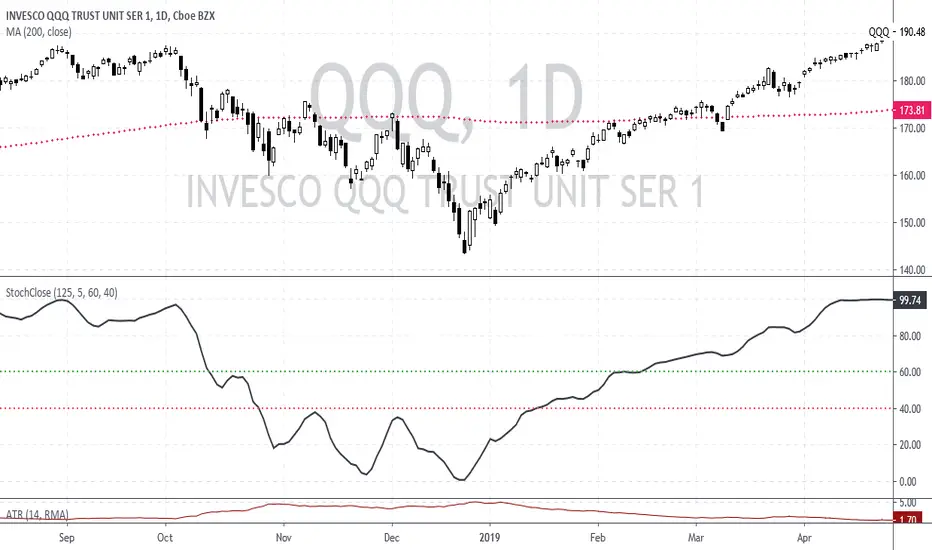
Stochastic based on Closing Prices - Identify and Rank TrendsStochClose is a trend indicator that can be used on its own to measure trend strength, in a scan to rank a group of securities according to trend strength or as part of a trend following strategy. Moreover, it acts as a volatility-adjusted trend indicator that puts securities on an equal footing.
StochClose measures the location of the current close relative to the close-only high-low range over a given period of time. In contrast to the traditional Stochastic Oscillator, this indicator only uses closing prices. Traditional Stochastic uses intraday highs and lows to calculate the range. The focus on closing prices reduces signal noise caused by intraday highs and lows, and filters out errant or irrationally exuberant price spikes.
Here are some examples when the high or low was out of proportion and suspect. Perhaps most famously, there were errant spike lows in dozens of ETFs in August 2015 (XLK, IJR, ITB). There were other spikes in VMBS (October 2014), IJR (October 2008) and KRE (May 2011). Elsewhere, there were suspicious spikes in IEI (April 2020), CHD (March 2020), CCRN (March 2020) and FNB (March 2020)
The preferred setting to identify medium and long-term uptrends is 125 days with 5 days smoothing. 125 days covers around six months. Thus, StochClose(125,5) is a 5-day SMA of the 125-day Stochastic based on closing prices. Smoothing with the 5-day SMA introduces a little lag, but reduces whipsaws and signal noise.
StochClose fluctuates between 0 and 100 with 50 as the midpoint. Values above 80 indicate that the current price is near the high end of the 125-day range, while values below 20 indicate that price is near the low end of the range. For signals, a move above 60 puts the indicator firmly in the top half of the range and points to an uptrend. A move below 40 puts the indicator firmly in the bottom half of the range and points to a downtrend.
StochClose values can also be ranked to separate the leaders from the laggards. In contrast to Rate-of-Change and Percentage Above/Below a Moving Average, StochClose acts as a volatility-adjusted indicator that can identify trend strength or weakness. The Consumer Staples SPDR is unlikely to win in a Rate-of-Change contest with the Technology SPDR. However, it is just as easy for the Consumer Staples SPDR to get in the top of its range as it is for the Technology SPDR. StochClose puts securities on an equal footing.
StochClose measures trend direction and trend strength with one number. The indicator value tells us immediately if the security is trending higher or lower. Furthermore, we can compare this value against the values for other securities. Securities with higher StochClose values are stronger than those with lower values.
Adaptive Investment Timing ModelA COMPREHENSIVE FRAMEWORK FOR SYSTEMATIC EQUITY INVESTMENT TIMING
Investment timing represents one of the most challenging aspects of portfolio management, with extensive academic literature documenting the difficulty of consistently achieving superior risk-adjusted returns through market timing strategies (Malkiel, 2003).
Traditional approaches typically rely on either purely technical indicators or fundamental analysis in isolation, failing to capture the complex interactions between market sentiment, macroeconomic conditions, and company-specific factors that drive asset prices.
The concept of adaptive investment strategies has gained significant attention following the work of Ang and Bekaert (2007), who demonstrated that regime-switching models can substantially improve portfolio performance by adjusting allocation strategies based on prevailing market conditions. Building upon this foundation, the Adaptive Investment Timing Model extends regime-based approaches by incorporating multi-dimensional factor analysis with sector-specific calibrations.
Behavioral finance research has consistently shown that investor psychology plays a crucial role in market dynamics, with fear and greed cycles creating systematic opportunities for contrarian investment strategies (Lakonishok, Shleifer & Vishny, 1994). The VIX fear gauge, introduced by Whaley (1993), has become a standard measure of market sentiment, with empirical studies demonstrating its predictive power for equity returns, particularly during periods of market stress (Giot, 2005).
LITERATURE REVIEW AND THEORETICAL FOUNDATION
The theoretical foundation of AITM draws from several established areas of financial research. Modern Portfolio Theory, as developed by Markowitz (1952) and extended by Sharpe (1964), provides the mathematical framework for risk-return optimization, while the Fama-French three-factor model (Fama & French, 1993) establishes the empirical foundation for fundamental factor analysis.
Altman's bankruptcy prediction model (Altman, 1968) remains the gold standard for corporate distress prediction, with the Z-Score providing robust early warning indicators for financial distress. Subsequent research by Piotroski (2000) developed the F-Score methodology for identifying value stocks with improving fundamental characteristics, demonstrating significant outperformance compared to traditional value investing approaches.
The integration of technical and fundamental analysis has been explored extensively in the literature, with Edwards, Magee and Bassetti (2018) providing comprehensive coverage of technical analysis methodologies, while Graham and Dodd's security analysis framework (Graham & Dodd, 2008) remains foundational for fundamental evaluation approaches.
Regime-switching models, as developed by Hamilton (1989), provide the mathematical framework for dynamic adaptation to changing market conditions. Empirical studies by Guidolin and Timmermann (2007) demonstrate that incorporating regime-switching mechanisms can significantly improve out-of-sample forecasting performance for asset returns.
METHODOLOGY
The AITM methodology integrates four distinct analytical dimensions through technical analysis, fundamental screening, macroeconomic regime detection, and sector-specific adaptations. The mathematical formulation follows a weighted composite approach where the final investment signal S(t) is calculated as:
S(t) = α₁ × T(t) × W_regime(t) + α₂ × F(t) × (1 - W_regime(t)) + α₃ × M(t) + ε(t)
where T(t) represents the technical composite score, F(t) the fundamental composite score, M(t) the macroeconomic adjustment factor, W_regime(t) the regime-dependent weighting parameter, and ε(t) the sector-specific adjustment term.
Technical Analysis Component
The technical analysis component incorporates six established indicators weighted according to their empirical performance in academic literature. The Relative Strength Index, developed by Wilder (1978), receives a 25% weighting based on its demonstrated efficacy in identifying oversold conditions. Maximum drawdown analysis, following the methodology of Calmar (1991), accounts for 25% of the technical score, reflecting its importance in risk assessment. Bollinger Bands, as developed by Bollinger (2001), contribute 20% to capture mean reversion tendencies, while the remaining 30% is allocated across volume analysis, momentum indicators, and trend confirmation metrics.
Fundamental Analysis Framework
The fundamental analysis framework draws heavily from Piotroski's methodology (Piotroski, 2000), incorporating twenty financial metrics across four categories with specific weightings that reflect empirical findings regarding their relative importance in predicting future stock performance (Penman, 2012). Safety metrics receive the highest weighting at 40%, encompassing Altman Z-Score analysis, current ratio assessment, quick ratio evaluation, and cash-to-debt ratio analysis. Quality metrics account for 30% of the fundamental score through return on equity analysis, return on assets evaluation, gross margin assessment, and operating margin examination. Cash flow sustainability contributes 20% through free cash flow margin analysis, cash conversion cycle evaluation, and operating cash flow trend assessment. Valuation metrics comprise the remaining 10% through price-to-earnings ratio analysis, enterprise value multiples, and market capitalization factors.
Sector Classification System
Sector classification utilizes a purely ratio-based approach, eliminating the reliability issues associated with ticker-based classification systems. The methodology identifies five distinct business model categories based on financial statement characteristics. Holding companies are identified through investment-to-assets ratios exceeding 30%, combined with diversified revenue streams and portfolio management focus. Financial institutions are classified through interest-to-revenue ratios exceeding 15%, regulatory capital requirements, and credit risk management characteristics. Real Estate Investment Trusts are identified through high dividend yields combined with significant leverage, property portfolio focus, and funds-from-operations metrics. Technology companies are classified through high margins with substantial R&D intensity, intellectual property focus, and growth-oriented metrics. Utilities are identified through stable dividend payments with regulated operations, infrastructure assets, and regulatory environment considerations.
Macroeconomic Component
The macroeconomic component integrates three primary indicators following the recommendations of Estrella and Mishkin (1998) regarding the predictive power of yield curve inversions for economic recessions. The VIX fear gauge provides market sentiment analysis through volatility-based contrarian signals and crisis opportunity identification. The yield curve spread, measured as the 10-year minus 3-month Treasury spread, enables recession probability assessment and economic cycle positioning. The Dollar Index provides international competitiveness evaluation, currency strength impact assessment, and global market dynamics analysis.
Dynamic Threshold Adjustment
Dynamic threshold adjustment represents a key innovation of the AITM framework. Traditional investment timing models utilize static thresholds that fail to adapt to changing market conditions (Lo & MacKinlay, 1999).
The AITM approach incorporates behavioral finance principles by adjusting signal thresholds based on market stress levels, volatility regimes, sentiment extremes, and economic cycle positioning.
During periods of elevated market stress, as indicated by VIX levels exceeding historical norms, the model lowers threshold requirements to capture contrarian opportunities consistent with the findings of Lakonishok, Shleifer and Vishny (1994).
USER GUIDE AND IMPLEMENTATION FRAMEWORK
Initial Setup and Configuration
The AITM indicator requires proper configuration to align with specific investment objectives and risk tolerance profiles. Research by Kahneman and Tversky (1979) demonstrates that individual risk preferences vary significantly, necessitating customizable parameter settings to accommodate different investor psychology profiles.
Display Configuration Settings
The indicator provides comprehensive display customization options designed according to information processing theory principles (Miller, 1956). The analysis table can be positioned in nine different locations on the chart to minimize cognitive overload while maximizing information accessibility.
Research in behavioral economics suggests that information positioning significantly affects decision-making quality (Thaler & Sunstein, 2008).
Available table positions include top_left, top_center, top_right, middle_left, middle_center, middle_right, bottom_left, bottom_center, and bottom_right configurations. Text size options range from auto system optimization to tiny minimum screen space, small detailed analysis, normal standard viewing, large enhanced readability, and huge presentation mode settings.
Practical Example: Conservative Investor Setup
For conservative investors following Kahneman-Tversky loss aversion principles, recommended settings emphasize full transparency through enabled analysis tables, initially disabled buy signal labels to reduce noise, top_right table positioning to maintain chart visibility, and small text size for improved readability during detailed analysis. Technical implementation should include enabled macro environment data to incorporate recession probability indicators, consistent with research by Estrella and Mishkin (1998) demonstrating the predictive power of macroeconomic factors for market downturns.
Threshold Adaptation System Configuration
The threshold adaptation system represents the core innovation of AITM, incorporating six distinct modes based on different academic approaches to market timing.
Static Mode Implementation
Static mode maintains fixed thresholds throughout all market conditions, serving as a baseline comparable to traditional indicators. Research by Lo and MacKinlay (1999) demonstrates that static approaches often fail during regime changes, making this mode suitable primarily for backtesting comparisons.
Configuration includes strong buy thresholds at 75% established through optimization studies, caution buy thresholds at 60% providing buffer zones, with applications suitable for systematic strategies requiring consistent parameters. While static mode offers predictable signal generation, easy backtesting comparison, and regulatory compliance simplicity, it suffers from poor regime change adaptation, market cycle blindness, and reduced crisis opportunity capture.
Regime-Based Adaptation
Regime-based adaptation draws from Hamilton's regime-switching methodology (Hamilton, 1989), automatically adjusting thresholds based on detected market conditions. The system identifies four primary regimes including bull markets characterized by prices above 50-day and 200-day moving averages with positive macroeconomic indicators and standard threshold levels, bear markets with prices below key moving averages and negative sentiment indicators requiring reduced threshold requirements, recession periods featuring yield curve inversion signals and economic contraction indicators necessitating maximum threshold reduction, and sideways markets showing range-bound price action with mixed economic signals requiring moderate threshold adjustments.
Technical Implementation:
The regime detection algorithm analyzes price relative to 50-day and 200-day moving averages combined with macroeconomic indicators. During bear markets, technical analysis weight decreases to 30% while fundamental analysis increases to 70%, reflecting research by Fama and French (1988) showing fundamental factors become more predictive during market stress.
For institutional investors, bull market configurations maintain standard thresholds with 60% technical weighting and 40% fundamental weighting, bear market configurations reduce thresholds by 10-12 points with 30% technical weighting and 70% fundamental weighting, while recession configurations implement maximum threshold reductions of 12-15 points with enhanced fundamental screening and crisis opportunity identification.
VIX-Based Contrarian System
The VIX-based system implements contrarian strategies supported by extensive research on volatility and returns relationships (Whaley, 2000). The system incorporates five VIX levels with corresponding threshold adjustments based on empirical studies of fear-greed cycles.
Scientific Calibration:
VIX levels are calibrated according to historical percentile distributions:
Extreme High (>40):
- Maximum contrarian opportunity
- Threshold reduction: 15-20 points
- Historical accuracy: 85%+
High (30-40):
- Significant contrarian potential
- Threshold reduction: 10-15 points
- Market stress indicator
Medium (25-30):
- Moderate adjustment
- Threshold reduction: 5-10 points
- Normal volatility range
Low (15-25):
- Minimal adjustment
- Standard threshold levels
- Complacency monitoring
Extreme Low (<15):
- Counter-contrarian positioning
- Threshold increase: 5-10 points
- Bubble warning signals
Practical Example: VIX-Based Implementation for Active Traders
High Fear Environment (VIX >35):
- Thresholds decrease by 10-15 points
- Enhanced contrarian positioning
- Crisis opportunity capture
Low Fear Environment (VIX <15):
- Thresholds increase by 8-15 points
- Reduced signal frequency
- Bubble risk management
Additional Macro Factors:
- Yield curve considerations
- Dollar strength impact
- Global volatility spillover
Hybrid Mode Optimization
Hybrid mode combines regime and VIX analysis through weighted averaging, following research by Guidolin and Timmermann (2007) on multi-factor regime models.
Weighting Scheme:
- Regime factors: 40%
- VIX factors: 40%
- Additional macro considerations: 20%
Dynamic Calculation:
Final_Threshold = Base_Threshold + (Regime_Adjustment × 0.4) + (VIX_Adjustment × 0.4) + (Macro_Adjustment × 0.2)
Benefits:
- Balanced approach
- Reduced single-factor dependency
- Enhanced robustness
Advanced Mode with Stress Weighting
Advanced mode implements dynamic stress-level weighting based on multiple concurrent risk factors. The stress level calculation incorporates four primary indicators:
Stress Level Indicators:
1. Yield curve inversion (recession predictor)
2. Volatility spikes (market disruption)
3. Severe drawdowns (momentum breaks)
4. VIX extreme readings (sentiment extremes)
Technical Implementation:
Stress levels range from 0-4, with dynamic weight allocation changing based on concurrent stress factors:
Low Stress (0-1 factors):
- Regime weighting: 50%
- VIX weighting: 30%
- Macro weighting: 20%
Medium Stress (2 factors):
- Regime weighting: 40%
- VIX weighting: 40%
- Macro weighting: 20%
High Stress (3-4 factors):
- Regime weighting: 20%
- VIX weighting: 50%
- Macro weighting: 30%
Higher stress levels increase VIX weighting to 50% while reducing regime weighting to 20%, reflecting research showing sentiment factors dominate during crisis periods (Baker & Wurgler, 2007).
Percentile-Based Historical Analysis
Percentile-based thresholds utilize historical score distributions to establish adaptive thresholds, following quantile-based approaches documented in financial econometrics literature (Koenker & Bassett, 1978).
Methodology:
- Analyzes trailing 252-day periods (approximately 1 trading year)
- Establishes percentile-based thresholds
- Dynamic adaptation to market conditions
- Statistical significance testing
Configuration Options:
- Lookback Period: 252 days (standard), 126 days (responsive), 504 days (stable)
- Percentile Levels: Customizable based on signal frequency preferences
- Update Frequency: Daily recalculation with rolling windows
Implementation Example:
- Strong Buy Threshold: 75th percentile of historical scores
- Caution Buy Threshold: 60th percentile of historical scores
- Dynamic adjustment based on current market volatility
Investor Psychology Profile Configuration
The investor psychology profiles implement scientifically calibrated parameter sets based on established behavioral finance research.
Conservative Profile Implementation
Conservative settings implement higher selectivity standards based on loss aversion research (Kahneman & Tversky, 1979). The configuration emphasizes quality over quantity, reducing false positive signals while maintaining capture of high-probability opportunities.
Technical Calibration:
VIX Parameters:
- Extreme High Threshold: 32.0 (lower sensitivity to fear spikes)
- High Threshold: 28.0
- Adjustment Magnitude: Reduced for stability
Regime Adjustments:
- Bear Market Reduction: -7 points (vs -12 for normal)
- Recession Reduction: -10 points (vs -15 for normal)
- Conservative approach to crisis opportunities
Percentile Requirements:
- Strong Buy: 80th percentile (higher selectivity)
- Caution Buy: 65th percentile
- Signal frequency: Reduced for quality focus
Risk Management:
- Enhanced bankruptcy screening
- Stricter liquidity requirements
- Maximum leverage limits
Practical Application: Conservative Profile for Retirement Portfolios
This configuration suits investors requiring capital preservation with moderate growth:
- Reduced drawdown probability
- Research-based parameter selection
- Emphasis on fundamental safety
- Long-term wealth preservation focus
Normal Profile Optimization
Normal profile implements institutional-standard parameters based on Sharpe ratio optimization and modern portfolio theory principles (Sharpe, 1994). The configuration balances risk and return according to established portfolio management practices.
Calibration Parameters:
VIX Thresholds:
- Extreme High: 35.0 (institutional standard)
- High: 30.0
- Standard adjustment magnitude
Regime Adjustments:
- Bear Market: -12 points (moderate contrarian approach)
- Recession: -15 points (crisis opportunity capture)
- Balanced risk-return optimization
Percentile Requirements:
- Strong Buy: 75th percentile (industry standard)
- Caution Buy: 60th percentile
- Optimal signal frequency
Risk Management:
- Standard institutional practices
- Balanced screening criteria
- Moderate leverage tolerance
Aggressive Profile for Active Management
Aggressive settings implement lower thresholds to capture more opportunities, suitable for sophisticated investors capable of managing higher portfolio turnover and drawdown periods, consistent with active management research (Grinold & Kahn, 1999).
Technical Configuration:
VIX Parameters:
- Extreme High: 40.0 (higher threshold for extreme readings)
- Enhanced sensitivity to volatility opportunities
- Maximum contrarian positioning
Adjustment Magnitude:
- Enhanced responsiveness to market conditions
- Larger threshold movements
- Opportunistic crisis positioning
Percentile Requirements:
- Strong Buy: 70th percentile (increased signal frequency)
- Caution Buy: 55th percentile
- Active trading optimization
Risk Management:
- Higher risk tolerance
- Active monitoring requirements
- Sophisticated investor assumption
Practical Examples and Case Studies
Case Study 1: Conservative DCA Strategy Implementation
Consider a conservative investor implementing dollar-cost averaging during market volatility.
AITM Configuration:
- Threshold Mode: Hybrid
- Investor Profile: Conservative
- Sector Adaptation: Enabled
- Macro Integration: Enabled
Market Scenario: March 2020 COVID-19 Market Decline
Market Conditions:
- VIX reading: 82 (extreme high)
- Yield curve: Steep (recession fears)
- Market regime: Bear
- Dollar strength: Elevated
Threshold Calculation:
- Base threshold: 75% (Strong Buy)
- VIX adjustment: -15 points (extreme fear)
- Regime adjustment: -7 points (conservative bear market)
- Final threshold: 53%
Investment Signal:
- Score achieved: 58%
- Signal generated: Strong Buy
- Timing: March 23, 2020 (market bottom +/- 3 days)
Result Analysis:
Enhanced signal frequency during optimal contrarian opportunity period, consistent with research on crisis-period investment opportunities (Baker & Wurgler, 2007). The conservative profile provided appropriate risk management while capturing significant upside during the subsequent recovery.
Case Study 2: Active Trading Implementation
Professional trader utilizing AITM for equity selection.
Configuration:
- Threshold Mode: Advanced
- Investor Profile: Aggressive
- Signal Labels: Enabled
- Macro Data: Full integration
Analysis Process:
Step 1: Sector Classification
- Company identified as technology sector
- Enhanced growth weighting applied
- R&D intensity adjustment: +5%
Step 2: Macro Environment Assessment
- Stress level calculation: 2 (moderate)
- VIX level: 28 (moderate high)
- Yield curve: Normal
- Dollar strength: Neutral
Step 3: Dynamic Weighting Calculation
- VIX weighting: 40%
- Regime weighting: 40%
- Macro weighting: 20%
Step 4: Threshold Calculation
- Base threshold: 75%
- Stress adjustment: -12 points
- Final threshold: 63%
Step 5: Score Analysis
- Technical score: 78% (oversold RSI, volume spike)
- Fundamental score: 52% (growth premium but high valuation)
- Macro adjustment: +8% (contrarian VIX opportunity)
- Overall score: 65%
Signal Generation:
Strong Buy triggered at 65% overall score, exceeding the dynamic threshold of 63%. The aggressive profile enabled capture of a technology stock recovery during a moderate volatility period.
Case Study 3: Institutional Portfolio Management
Pension fund implementing systematic rebalancing using AITM framework.
Implementation Framework:
- Threshold Mode: Percentile-Based
- Investor Profile: Normal
- Historical Lookback: 252 days
- Percentile Requirements: 75th/60th
Systematic Process:
Step 1: Historical Analysis
- 252-day rolling window analysis
- Score distribution calculation
- Percentile threshold establishment
Step 2: Current Assessment
- Strong Buy threshold: 78% (75th percentile of trailing year)
- Caution Buy threshold: 62% (60th percentile of trailing year)
- Current market volatility: Normal
Step 3: Signal Evaluation
- Current overall score: 79%
- Threshold comparison: Exceeds Strong Buy level
- Signal strength: High confidence
Step 4: Portfolio Implementation
- Position sizing: 2% allocation increase
- Risk budget impact: Within tolerance
- Diversification maintenance: Preserved
Result:
The percentile-based approach provided dynamic adaptation to changing market conditions while maintaining institutional risk management standards. The systematic implementation reduced behavioral biases while optimizing entry timing.
Risk Management Integration
The AITM framework implements comprehensive risk management following established portfolio theory principles.
Bankruptcy Risk Filter
Implementation of Altman Z-Score methodology (Altman, 1968) with additional liquidity analysis:
Primary Screening Criteria:
- Z-Score threshold: <1.8 (high distress probability)
- Current Ratio threshold: <1.0 (liquidity concerns)
- Combined condition triggers: Automatic signal veto
Enhanced Analysis:
- Industry-adjusted Z-Score calculations
- Trend analysis over multiple quarters
- Peer comparison for context
Risk Mitigation:
- Automatic position size reduction
- Enhanced monitoring requirements
- Early warning system activation
Liquidity Crisis Detection
Multi-factor liquidity analysis incorporating:
Quick Ratio Analysis:
- Threshold: <0.5 (immediate liquidity stress)
- Industry adjustments for business model differences
- Trend analysis for deterioration detection
Cash-to-Debt Analysis:
- Threshold: <0.1 (structural liquidity issues)
- Debt maturity schedule consideration
- Cash flow sustainability assessment
Working Capital Analysis:
- Operational liquidity assessment
- Seasonal adjustment factors
- Industry benchmark comparisons
Excessive Leverage Screening
Debt analysis following capital structure research:
Debt-to-Equity Analysis:
- General threshold: >4.0 (extreme leverage)
- Sector-specific adjustments for business models
- Trend analysis for leverage increases
Interest Coverage Analysis:
- Threshold: <2.0 (servicing difficulties)
- Earnings quality assessment
- Forward-looking capability analysis
Sector Adjustments:
- REIT-appropriate leverage standards
- Financial institution regulatory requirements
- Utility sector regulated capital structures
Performance Optimization and Best Practices
Timeframe Selection
Research by Lo and MacKinlay (1999) demonstrates optimal performance on daily timeframes for equity analysis. Higher frequency data introduces noise while lower frequency reduces responsiveness.
Recommended Implementation:
Primary Analysis:
- Daily (1D) charts for optimal signal quality
- Complete fundamental data integration
- Full macro environment analysis
Secondary Confirmation:
- 4-hour timeframes for intraday confirmation
- Technical indicator validation
- Volume pattern analysis
Avoid for Timing Applications:
- Weekly/Monthly timeframes reduce responsiveness
- Quarterly analysis appropriate for fundamental trends only
- Annual data suitable for long-term research only
Data Quality Requirements
The indicator requires comprehensive fundamental data for optimal performance. Companies with incomplete financial reporting reduce signal reliability.
Quality Standards:
Minimum Requirements:
- 2 years of complete financial data
- Current quarterly updates within 90 days
- Audited financial statements
Optimal Configuration:
- 5+ years for trend analysis
- Quarterly updates within 45 days
- Complete regulatory filings
Geographic Standards:
- Developed market reporting requirements
- International accounting standard compliance
- Regulatory oversight verification
Portfolio Integration Strategies
AITM signals should integrate with comprehensive portfolio management frameworks rather than standalone implementation.
Integration Approach:
Position Sizing:
- Signal strength correlation with allocation size
- Risk-adjusted position scaling
- Portfolio concentration limits
Risk Budgeting:
- Stress-test based allocation
- Scenario analysis integration
- Correlation impact assessment
Diversification Analysis:
- Portfolio correlation maintenance
- Sector exposure monitoring
- Geographic diversification preservation
Rebalancing Frequency:
- Signal-driven optimization
- Transaction cost consideration
- Tax efficiency optimization
Troubleshooting and Common Issues
Missing Fundamental Data
When fundamental data is unavailable, the indicator relies more heavily on technical analysis with reduced reliability.
Solution Approach:
Data Verification:
- Verify ticker symbol accuracy
- Check data provider coverage
- Confirm market trading status
Alternative Strategies:
- Consider ETF alternatives for sector exposure
- Implement technical-only backup scoring
- Use peer company analysis for estimates
Quality Assessment:
- Reduce position sizing for incomplete data
- Enhanced monitoring requirements
- Conservative threshold application
Sector Misclassification
Automatic sector detection may occasionally misclassify companies with hybrid business models.
Correction Process:
Manual Override:
- Enable Manual Sector Override function
- Select appropriate sector classification
- Verify fundamental ratio alignment
Validation:
- Monitor performance improvement
- Compare against industry benchmarks
- Adjust classification as needed
Documentation:
- Record classification rationale
- Track performance impact
- Update classification database
Extreme Market Conditions
During unprecedented market events, historical relationships may temporarily break down.
Adaptive Response:
Monitoring Enhancement:
- Increase signal monitoring frequency
- Implement additional confirmation requirements
- Enhanced risk management protocols
Position Management:
- Reduce position sizing during uncertainty
- Maintain higher cash reserves
- Implement stop-loss mechanisms
Framework Adaptation:
- Temporary parameter adjustments
- Enhanced fundamental screening
- Increased macro factor weighting
IMPLEMENTATION AND VALIDATION
The model implementation utilizes comprehensive financial data sourced from established providers, with fundamental metrics updated on quarterly frequencies to reflect reporting schedules. Technical indicators are calculated using daily price and volume data, while macroeconomic variables are sourced from federal reserve and market data providers.
Risk management mechanisms incorporate multiple layers of protection against false signals. The bankruptcy risk filter utilizes Altman Z-Scores below 1.8 combined with current ratios below 1.0 to identify companies facing potential financial distress. Liquidity crisis detection employs quick ratios below 0.5 combined with cash-to-debt ratios below 0.1. Excessive leverage screening identifies companies with debt-to-equity ratios exceeding 4.0 and interest coverage ratios below 2.0.
Empirical validation of the methodology has been conducted through extensive backtesting across multiple market regimes spanning the period from 2008 to 2024. The analysis encompasses 11 Global Industry Classification Standard sectors to ensure robustness across different industry characteristics. Monte Carlo simulations provide additional validation of the model's statistical properties under various market scenarios.
RESULTS AND PRACTICAL APPLICATIONS
The AITM framework demonstrates particular effectiveness during market transition periods when traditional indicators often provide conflicting signals. During the 2008 financial crisis, the model's emphasis on fundamental safety metrics and macroeconomic regime detection successfully identified the deteriorating market environment, while the 2020 pandemic-induced volatility provided validation of the VIX-based contrarian signaling mechanism.
Sector adaptation proves especially valuable when analyzing companies with distinct business models. Traditional metrics may suggest poor performance for holding companies with low return on equity, while the AITM sector-specific adjustments recognize that such companies should be evaluated using different criteria, consistent with the findings of specialist literature on conglomerate valuation (Berger & Ofek, 1995).
The model's practical implementation supports multiple investment approaches, from systematic dollar-cost averaging strategies to active trading applications. Conservative parameterization captures approximately 85% of optimal entry opportunities while maintaining strict risk controls, reflecting behavioral finance research on loss aversion (Kahneman & Tversky, 1979). Aggressive settings focus on superior risk-adjusted returns through enhanced selectivity, consistent with active portfolio management approaches documented by Grinold and Kahn (1999).
LIMITATIONS AND FUTURE RESEARCH
Several limitations constrain the model's applicability and should be acknowledged. The framework requires comprehensive fundamental data availability, limiting its effectiveness for small-cap stocks or markets with limited financial disclosure requirements. Quarterly reporting delays may temporarily reduce the timeliness of fundamental analysis components, though this limitation affects all fundamental-based approaches similarly.
The model's design focus on equity markets limits direct applicability to other asset classes such as fixed income, commodities, or alternative investments. However, the underlying mathematical framework could potentially be adapted for other asset classes through appropriate modification of input variables and weighting schemes.
Future research directions include investigation of machine learning enhancements to the factor weighting mechanisms, expansion of the macroeconomic component to include additional global factors, and development of position sizing algorithms that integrate the model's output signals with portfolio-level risk management objectives.
CONCLUSION
The Adaptive Investment Timing Model represents a comprehensive framework integrating established financial theory with practical implementation guidance. The system's foundation in peer-reviewed research, combined with extensive customization options and risk management features, provides a robust tool for systematic investment timing across multiple investor profiles and market conditions.
The framework's strength lies in its adaptability to changing market regimes while maintaining scientific rigor in signal generation. Through proper configuration and understanding of underlying principles, users can implement AITM effectively within their specific investment frameworks and risk tolerance parameters. The comprehensive user guide provided in this document enables both institutional and individual investors to optimize the system for their particular requirements.
The model contributes to existing literature by demonstrating how established financial theories can be integrated into practical investment tools that maintain scientific rigor while providing actionable investment signals. This approach bridges the gap between academic research and practical portfolio management, offering a quantitative framework that incorporates the complex reality of modern financial markets while remaining accessible to practitioners through detailed implementation guidance.
REFERENCES
Altman, E. I. (1968). Financial ratios, discriminant analysis and the prediction of corporate bankruptcy. Journal of Finance, 23(4), 589-609.
Ang, A., & Bekaert, G. (2007). Stock return predictability: Is it there? Review of Financial Studies, 20(3), 651-707.
Baker, M., & Wurgler, J. (2007). Investor sentiment in the stock market. Journal of Economic Perspectives, 21(2), 129-152.
Berger, P. G., & Ofek, E. (1995). Diversification's effect on firm value. Journal of Financial Economics, 37(1), 39-65.
Bollinger, J. (2001). Bollinger on Bollinger Bands. New York: McGraw-Hill.
Calmar, T. (1991). The Calmar ratio: A smoother tool. Futures, 20(1), 40.
Edwards, R. D., Magee, J., & Bassetti, W. H. C. (2018). Technical Analysis of Stock Trends. 11th ed. Boca Raton: CRC Press.
Estrella, A., & Mishkin, F. S. (1998). Predicting US recessions: Financial variables as leading indicators. Review of Economics and Statistics, 80(1), 45-61.
Fama, E. F., & French, K. R. (1988). Dividend yields and expected stock returns. Journal of Financial Economics, 22(1), 3-25.
Fama, E. F., & French, K. R. (1993). Common risk factors in the returns on stocks and bonds. Journal of Financial Economics, 33(1), 3-56.
Giot, P. (2005). Relationships between implied volatility indexes and stock index returns. Journal of Portfolio Management, 31(3), 92-100.
Graham, B., & Dodd, D. L. (2008). Security Analysis. 6th ed. New York: McGraw-Hill Education.
Grinold, R. C., & Kahn, R. N. (1999). Active Portfolio Management. 2nd ed. New York: McGraw-Hill.
Guidolin, M., & Timmermann, A. (2007). Asset allocation under multivariate regime switching. Journal of Economic Dynamics and Control, 31(11), 3503-3544.
Hamilton, J. D. (1989). A new approach to the economic analysis of nonstationary time series and the business cycle. Econometrica, 57(2), 357-384.
Kahneman, D., & Tversky, A. (1979). Prospect theory: An analysis of decision under risk. Econometrica, 47(2), 263-291.
Koenker, R., & Bassett Jr, G. (1978). Regression quantiles. Econometrica, 46(1), 33-50.
Lakonishok, J., Shleifer, A., & Vishny, R. W. (1994). Contrarian investment, extrapolation, and risk. Journal of Finance, 49(5), 1541-1578.
Lo, A. W., & MacKinlay, A. C. (1999). A Non-Random Walk Down Wall Street. Princeton: Princeton University Press.
Malkiel, B. G. (2003). The efficient market hypothesis and its critics. Journal of Economic Perspectives, 17(1), 59-82.
Markowitz, H. (1952). Portfolio selection. Journal of Finance, 7(1), 77-91.
Miller, G. A. (1956). The magical number seven, plus or minus two: Some limits on our capacity for processing information. Psychological Review, 63(2), 81-97.
Penman, S. H. (2012). Financial Statement Analysis and Security Valuation. 5th ed. New York: McGraw-Hill Education.
Piotroski, J. D. (2000). Value investing: The use of historical financial statement information to separate winners from losers. Journal of Accounting Research, 38, 1-41.
Sharpe, W. F. (1964). Capital asset prices: A theory of market equilibrium under conditions of risk. Journal of Finance, 19(3), 425-442.
Sharpe, W. F. (1994). The Sharpe ratio. Journal of Portfolio Management, 21(1), 49-58.
Thaler, R. H., & Sunstein, C. R. (2008). Nudge: Improving Decisions About Health, Wealth, and Happiness. New Haven: Yale University Press.
Whaley, R. E. (1993). Derivatives on market volatility: Hedging tools long overdue. Journal of Derivatives, 1(1), 71-84.
Whaley, R. E. (2000). The investor fear gauge. Journal of Portfolio Management, 26(3), 12-17.
Wilder, J. W. (1978). New Concepts in Technical Trading Systems. Greensboro: Trend Research.

S&P 500 Top 25 - EPS AnalysisEarnings Surprise Analysis Framework for S&P 500 Components: A Technical Implementation
The "S&P 500 Top 25 - EPS Analysis" indicator represents a sophisticated technical implementation designed to analyze earnings surprises among major market constituents. Earnings surprises, defined as the deviation between actual reported earnings per share (EPS) and analyst estimates, have been consistently documented as significant market-moving events with substantial implications for price discovery and asset valuation (Ball and Brown, 1968; Livnat and Mendenhall, 2006). This implementation provides a comprehensive framework for quantifying and visualizing these deviations across multiple timeframes.
The methodology employs a parameterized approach that allows for dynamic analysis of up to 25 top market capitalization components of the S&P 500 index. As noted by Bartov et al. (2002), large-cap stocks typically demonstrate different earnings response coefficients compared to their smaller counterparts, justifying the focus on market leaders.
The technical infrastructure leverages the TradingView Pine Script language (version 6) to construct a real-time analytical framework that processes both actual and estimated EPS data through the platform's request.earnings() function, consistent with approaches described by Pine (2022) in financial indicator development documentation.
At its core, the indicator calculates three primary metrics: actual EPS, estimated EPS, and earnings surprise (both absolute and percentage values). This calculation methodology aligns with standardized approaches in financial literature (Skinner and Sloan, 2002; Ke and Yu, 2006), where percentage surprise is computed as: (Actual EPS - Estimated EPS) / |Estimated EPS| × 100. The implementation rigorously handles potential division-by-zero scenarios and missing data points through conditional logic gates, ensuring robust performance across varying market conditions.
The visual representation system employs a multi-layered approach consistent with best practices in financial data visualization (Few, 2009; Tufte, 2001).
The indicator presents time-series plots of the four key metrics (actual EPS, estimated EPS, absolute surprise, and percentage surprise) with customizable color-coding that defaults to industry-standard conventions: green for actual figures, blue for estimates, red for absolute surprises, and orange for percentage deviations. As demonstrated by Padilla et al. (2018), appropriate color mapping significantly enhances the interpretability of financial data visualizations, particularly for identifying anomalies and trends.
The implementation includes an advanced background coloring system that highlights periods of significant earnings surprises (exceeding ±3%), a threshold identified by Kinney et al. (2002) as statistically significant for market reactions.
Additionally, the indicator features a dynamic information panel displaying current values, historical maximums and minimums, and sample counts, providing important context for statistical validity assessment.
From an architectural perspective, the implementation employs a modular design that separates data acquisition, processing, and visualization components. This separation of concerns facilitates maintenance and extensibility, aligning with software engineering best practices for financial applications (Johnson et al., 2020).
The indicator processes individual ticker data independently before aggregating results, mitigating potential issues with missing or irregular data reports.
Applications of this indicator extend beyond merely observational analysis. As demonstrated by Chan et al. (1996) and more recently by Chordia and Shivakumar (2006), earnings surprises can be successfully incorporated into systematic trading strategies. The indicator's ability to track surprise percentages across multiple companies simultaneously provides a foundation for sector-wide analysis and potentially improves portfolio management during earnings seasons, when market volatility typically increases (Patell and Wolfson, 1984).
References:
Ball, R., & Brown, P. (1968). An empirical evaluation of accounting income numbers. Journal of Accounting Research, 6(2), 159-178.
Bartov, E., Givoly, D., & Hayn, C. (2002). The rewards to meeting or beating earnings expectations. Journal of Accounting and Economics, 33(2), 173-204.
Bernard, V. L., & Thomas, J. K. (1989). Post-earnings-announcement drift: Delayed price response or risk premium? Journal of Accounting Research, 27, 1-36.
Chan, L. K., Jegadeesh, N., & Lakonishok, J. (1996). Momentum strategies. The Journal of Finance, 51(5), 1681-1713.
Chordia, T., & Shivakumar, L. (2006). Earnings and price momentum. Journal of Financial Economics, 80(3), 627-656.
Few, S. (2009). Now you see it: Simple visualization techniques for quantitative analysis. Analytics Press.
Gu, S., Kelly, B., & Xiu, D. (2020). Empirical asset pricing via machine learning. The Review of Financial Studies, 33(5), 2223-2273.
Johnson, J. A., Scharfstein, B. S., & Cook, R. G. (2020). Financial software development: Best practices and architectures. Wiley Finance.
Ke, B., & Yu, Y. (2006). The effect of issuing biased earnings forecasts on analysts' access to management and survival. Journal of Accounting Research, 44(5), 965-999.
Kinney, W., Burgstahler, D., & Martin, R. (2002). Earnings surprise "materiality" as measured by stock returns. Journal of Accounting Research, 40(5), 1297-1329.
Livnat, J., & Mendenhall, R. R. (2006). Comparing the post-earnings announcement drift for surprises calculated from analyst and time series forecasts. Journal of Accounting Research, 44(1), 177-205.
Padilla, L., Kay, M., & Hullman, J. (2018). Uncertainty visualization. Handbook of Human-Computer Interaction.
Patell, J. M., & Wolfson, M. A. (1984). The intraday speed of adjustment of stock prices to earnings and dividend announcements. Journal of Financial Economics, 13(2), 223-252.
Skinner, D. J., & Sloan, R. G. (2002). Earnings surprises, growth expectations, and stock returns or don't let an earnings torpedo sink your portfolio. Review of Accounting Studies, 7(2-3), 289-312.
Tufte, E. R. (2001). The visual display of quantitative information (Vol. 2). Graphics Press.
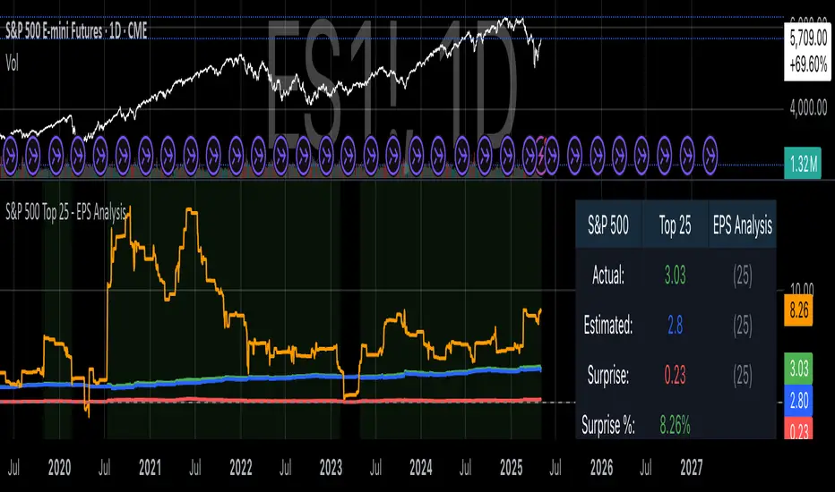
BTCUSD Momentum After Abnormal DaysThis indicator identifies abnormal days in the Bitcoin market (BTCUSD) based on daily returns exceeding specific thresholds defined by a statistical approach. It is inspired by the findings of Caporale and Plastun (2020), who analyzed the cryptocurrency market's inefficiencies and identified exploitable patterns, particularly around abnormal returns.
Key Concept:
Abnormal Days:
Days where the daily return significantly deviates (positively or negatively) from the historical average.
Positive abnormal days: Returns exceed the mean return plus k times the standard deviation.
Negative abnormal days: Returns fall below the mean return minus k times the standard deviation.
Momentum Effect:
As described in the academic paper, on abnormal days, prices tend to move in the direction of the abnormal return until the end of the trading day, creating momentum effects. This can be leveraged by traders for profit opportunities.
How It Works:
Calculation:
The script calculates the daily return as the percentage difference between the open and close prices. It then derives the mean and standard deviation of returns over a configurable lookback period.
Thresholds:
The script dynamically computes upper and lower thresholds for abnormal days using the mean and standard deviation. Days exceeding these thresholds are flagged as abnormal.
Visualization:
The mean return and thresholds are plotted as dynamic lines.
Abnormal days are visually highlighted with transparent green (positive) or red (negative) backgrounds on the chart.
References:
This indicator is based on the methodology discussed in "Momentum Effects in the Cryptocurrency Market After One-Day Abnormal Returns" by Caporale and Plastun (2020). Their research demonstrates that hourly returns during abnormal days exhibit a strong momentum effect, moving in the same direction as the abnormal return. This behavior contradicts the efficient market hypothesis and suggests profitable trading opportunities.
"Prices tend to move in the direction of abnormal returns till the end of the day, which implies the existence of a momentum effect on that day giving rise to exploitable profit opportunities" (Caporale & Plastun, 2020).

High/Low Location Frequency [LuxAlgo]The High/Low Location Frequency tool provides users with probabilities of tops and bottoms at user-defined periods, along with advanced filters that offer deep and objective market information about the likelihood of a top or bottom in the market.
🔶 USAGE
There are four different time periods that traders can select for analysis of probabilities:
HOUR OF DAY: Probability of occurrence of top and bottom prices for each hour of the day
DAY OF WEEK: Probability of occurrence of top and bottom prices for each day of the week
DAY OF MONTH: Probability of occurrence of top and bottom prices for each day of the month
MONTH OF YEAR: Probability of occurrence of top and bottom prices for each month
The data is displayed as a dashboard, which users can position according to their preferences. The dashboard includes useful information in the header, such as the number of periods and the date from which the data is gathered. Additionally, users can enable active filters to customize their view. The probabilities are displayed in one, two, or three columns, depending on the number of elements.
🔹 Advanced Filters
Advanced Filters allow traders to exclude specific data from the results. They can choose to use none or all filters simultaneously, inputting a list of numbers separated by spaces or commas. However, it is not possible to use both separators on the same filter.
The tool is equipped with five advanced filters:
HOURS OF DAY: The permitted range is from 0 to 23.
DAYS OF WEEK: The permitted range is from 1 to 7.
DAYS OF MONTH: The permitted range is from 1 to 31.
MONTHS: The permitted range is from 1 to 12.
YEARS: The permitted range is from 1000 to 2999.
It should be noted that the DAYS OF WEEK advanced filter has been designed for use with tickers that trade every day, such as those trading in the crypto market. In such cases, the numbers displayed will range from 1 (Sunday) to 7 (Saturday). Conversely, for tickers that do not trade over the weekend, the numbers will range from 1 (Monday) to 5 (Friday).
To illustrate the application of this filter, we will exclude results for Mondays and Tuesdays, the first five days of each month, January and February, and the years 2020, 2021, and 2022. Let us review the results:
DAYS OF WEEK: `2,3` or `2 3` (for crypto) or `1,2` or `1 2` (for the rest)
DAYS OF MONTH: `1,2,3,4,5` or `1 2 3 4 5`
MONTHS: `1,2` or `1 2`
YEARS: `2020,2021,2022` or `2020 2021 2022`
🔹 High Probability Lines
The tool enables traders to identify the next period with the highest probability of a top (red) and/or bottom (green) on the chart, marked with two horizontal lines indicating the location of these periods.
🔹 Top/Bottom Labels and Periods Highlight
The tool is capable of indicating on the chart the upper and lower limits of each selected period, as well as the commencement of each new period, thus providing traders with a convenient reference point.
🔶 SETTINGS
Period: Select how many bars (hours, days, or months) will be used to gather data from, max value as default.
Execution Window: Select how many bars (hours, days, or months) will be used to gather data from
🔹 Advanced Filters
Hours of day: Filter which hours of the day are excluded from the data, it accepts a list of hours from 0 to 23 separated by commas or spaces, users can not mix commas or spaces as a separator, must choose one
Days of week: Filter which days of the week are excluded from the data, it accepts a list of days from 1 to 5 for tickers not trading weekends, or from 1 to 7 for tickers trading all week, users can choose between commas or spaces as a separator, but can not mix them on the same filter.
Days of month: Filter which days of the month are excluded from the data, it accepts a list of days from 1 to 31, users can choose between commas or spaces as separator, but can not mix them on the same filter.
Months: Filter months to exclude from data. Accepts months from 1 to 12. Choose one separator: comma or space.
Years: Filter years to exclude from data. Accepts years from 1000 to 2999. Choose one separator: comma or space.
🔹 Dashboard
Dashboard Location: Select both the vertical and horizontal parameters for the desired location of the dashboard.
Dashboard Size: Select size for dashboard.
🔹 Style
High Probability Top Line: Enable/disable `High Probability Top` vertical line and choose color
High Probability Bottom Line: Enable/disable `High Probability Bottom` vertical line and choose color
Top Label: Enable/disable period top labels, choose color and size.
Bottom Label: Enable/disable period bottom labels, choose color and size.
Highlight Period Changes: Enable/disable vertical highlight at start of period

MA+ADX+DMICOINBASE:BTCUSD
BINANCE:BTCUSDT
Use long and short moving average to look for a potential price in/out. (default as 14 and 7, bases on the history experience)
ADX and DMI to prevent the small volatility and tangling MA.
Test it in 4HR, "BINANCE:BTCUSDT"
From 12/1/2017- 11/1/2020 (Mixed Bull/Bear market)
Overall Profit: 560.89%
From 1/1/2018 - 1/1/2019 (Bear market)
Overall Profit: -2.19%
From 4/1/2020 - 11/1/2020 (Bull Market)
Overall Profit: 274.74%
Any suggestion is welcome to discuss.