Volume Weighted LR Z ScoreThis indicator calculates the Volume Weighted Linear Regression
Z-Score (VWLRZS). Unlike a standard Z-Score which measures
deviation from a static mean, this oscillator measures the
statistical distance of price from a dynamic Volume-Weighted
Linear Regression Line (Analysis of Residuals).
Key Features:
1. **Volatility Decomposition:** The indicator separates volatility
based on the 'Estimate Bar Statistics' option.
- **Standard Mode (`Estimate Bar Statistics` = OFF):** Calculates
standard Regression Residuals using the selected `Source`
for both the regression line (baseline) and the signal.
- **Decomposition Mode (`Estimate Bar Statistics` = ON):**
Uses a hybrid statistical approach:
a) **The Model (Baseline):** Uses an estimator to calculate
the 'within-bar' mean and fits the Linear Regression
through these statistical centers. This creates a
stable, trend-following expectation model.
b) **The Signal (Observation):** Compares the actual `Source`
(e.g., Close) against this regression line.
(Result: A Z-Score that measures deviations from the current
trend slope rather than a flat average).
2. **Visual Decomposition Logic:** Total Standard Deviation (of
Residuals) is the primary metric displayed. Since Standard
Deviations are not linearly additive (sqrt(a+b) != sqrt(a)+sqrt(b)),
this indicator calculates the *exact* Total Z-Score and partitions
the area underneath based on the Variance Ratio. This ensures the
displayed total volatility remains mathematically accurate while
showing relative composition.
3. **Normalization (Exponential Regression):** Includes an optional
'Normalize' mode. When enabled, the indicator calculates the
Linear Regression on logarithmic data. Mathematically, this
transforms the baseline into an **Exponential Regression Curve**,
making it ideal for analyzing assets with compounding growth
characteristics (constant percentage trend).
4. **Full Divergence Suite (Class A, B, C):** The indicator's
primary feature is its integrated divergence engine. It
automatically detects and plots all three major divergence
classes between price and the Z-Score:
- Regular (A): Signals potential trend exhaustion and reversals.
- Hidden (B): Signals potential trend continuations during pullbacks.
- Exaggerated (C): Signals weakness at double tops/bottoms.
5. **Divergence Filtering and Visualization:**
- **Price Tolerance Filter:** Divergence detection is enhanced
with a percentage-based price tolerance (`pivPrcTol`) to
filter out insignificant market noise, leading to more
robust signals.
- **Persistent Visualization:** Divergence markers are plotted
for the entire duration of the signal and are visually
anchored to the oscillator level of the confirming pivot.
- **Flexible Pivot Algorithms:** Supports various underlying
mathematical models for pivot detection provided by the
core library
6. **Note on Confirmation (Lag):** Divergence signals rely on a
pivot confirmation method to ensure they do not repaint.
- The **Start** of a divergence is only detected *after* the
confirming pivot is fully formed (a delay based on
`Pivot Right Bars`).
- The **End** of a divergence is detected either instantly
(if the signal is invalidated by price action) or with
a delay (when a new, non-divergent pivot is confirmed).
7. **Multi-Timeframe (MTF) Capability:**
- **MTF Calculation:** The Z-Score line *itself* can be calculated on a
higher timeframe, with standard options to handle gaps
(`Fill Gaps`) and prevent repainting (`Wait for...`).
- **Limitation:** The Divergence detection engine (`pivDiv`)
is designed for the active timeframe. Using it in MTF mode
is not recommended as step-data can lead to inaccurate
pivot detection.
8. **Integrated Alerts:** Includes a comprehensive set of built-in
alerts for the Z-Score crossing the neutral line, the configured
Threshold levels, and the start/end of all divergence types.
---
**DISCLAIMER**
1. **For Informational/Educational Use Only:** This indicator is
provided for informational and educational purposes only. It does
not constitute financial, investment, or trading advice, nor is
it a recommendation to buy or sell any asset.
2. **Use at Your Own Risk:** All trading decisions you make based on
the information or signals generated by this indicator are made
solely at your own risk.
3. **No Guarantee of Performance:** Past performance is not an
indicator of future results. The author makes no guarantee
regarding the accuracy of the signals or future profitability.
4. **No Liability:** The author shall not be held liable for any
financial losses or damages incurred directly or indirectly from
the use of this indicator.
5. **Signals Are Not Recommendations:** The alerts and visual signals
(e.g., crossovers) generated by this tool are not direct
recommendations to buy or sell. They are technical observations
for your own analysis and consideration.
Cari dalam skrip untuk "Exponential"

ED by bigmmED by bigmm identifies significant price divergences from the 200-period Exponential Moving Average (EMA) by analyzing closing and opening price extremes. This tool marks the three most recent candles with the largest percentage deviations.
Key Features
EMA200 Analysis: Uses the 200-period Exponential Moving Average as the primary reference level for measuring price deviations
Deviation Calculation: Computes percentage-based deviations for both closing (below EMA) and opening (above EMA) prices
Top 3 Extremes: Identifies and marks only the three most recent maximum deviations for each direction
Visual Simplicity: Uses minimalistic green and red dots for clear visual identification without chart clutter
Historical Analysis: Evaluates the last 1440 bars (approximately 3 years on daily timeframe) to find significant deviation patterns
Recommended Usage
Best used on higher timeframes (H4, D1, W1) for the following reasons:
Reduced Noise: Higher timeframes filter out market noise and provide cleaner deviation signals
Trend Context: EMA200 carries more significance on daily and weekly charts as a major trend indicator
Strategic Signals: Extreme deviations on higher timeframes often correspond to important support/resistance levels and potential reversal zones
Reduced False Signals: Longer timeframes minimize whipsaws and provide more reliable extreme readings
Position Trading: Ideal for swing traders and position traders who base decisions on daily or weekly price action

4 Fibonacci EMAsAdd 4 Fibonacci EMAs to your charts with one indicator.
Configureable by value, so they don't necessarily have to use Fibonacci numbers, and by colors.

ONE RING 8 MA Bands with RaysCycle analysis tool ...
MAs: Eight moving averages (MA1–MA8) with customizable lengths, types (RMA, WMA, EMA, SMA), and offsets
Bands: Upper/lower bands for each MA, calculated based on final_pctX (Percentage mode) or final_ptsX (Points mode), scaled by multiplier
Rays: Forward-projected lines for bands, with customizable start points, styles (Solid, Dashed, Dotted), and lengths (up to 500 bars)
Band Choices
Manual: Uses individual inputs for band offsets
Uniform: Sets all offsets to base_pct (e.g., 0.1%) or base_pts (e.g., 0.1 points)
Linear: Scales linearly (e.g., base_pct * 1, base_pct * 2, base_pct * 3 ..., base_pct * 8)
Exponential: Scales exponentially (e.g., base_pct * 1, base_pct * 2, base_pct * 4, base_pct * 8 ..., base_pct * 128)
ATR-Based: Offsets are derived from the Average True Range (ATR), scaled by a linear factor. Dynamic bands that adapt to market conditions, useful for breakout or mean-reversion strategies. (final_pct1 = base_pct * atr, final_pct2 = base_pct * atr * 2, ..., final_pct8 = base_pct * atr * 8)
Geometric: Offsets follow a geometric progression (e.g., base_pct * r^0, base_pct * r^1, base_pct * r^2, ..., where r is a ratio like 1.5) This is less aggressive than Exponential (which uses powers of 2) and provides a smoother progression.
Example: If base_pct = 0.1, r = 1.5, then final_pct1 = 0.1%, final_pct2 = 0.15%, final_pct3 = 0.225%, ..., final_pct8 ≈ 1.71%
Harmonic: Offsets are based on harmonic flavored ratios. final_pctX = base_pct * X / (9 - X), final_ptsX = base_pts * X / (9 - X) for X = 1 to 8 This creates a harmonic-like progression where offsets increase non-linearly, ensuring MA8 bands are wider than MA1 bands, and avoids duplicating the Linear choice above.
Ex. offsets for base_pct = 0.1: MA1: ±0.0125% (0.1 * 1/8), MA2: ±0.0286% (0.1 * 2/7), MA3: ±0.05% (0.1 * 3/6), MA4: ±0.08% (0.1 * 4/5), MA5: ±0.125% (0.1 * 5/4), MA6: ±0.2% (0.1 * 6/3), MA7: ±0.35% (0.1 * 7/2), MA8: ±0.8% (0.1 * 8/1)
Square Root: Offsets grow with the square root of the band index (e.g., base_pct * sqrt(1), base_pct * sqrt(2), ..., base_pct * sqrt(8)). This creates a gradual widening, less aggressive than Linear or Exponential. Set final_pct1 = base_pct * sqrt(1), final_pct2 = base_pct * sqrt(2), ..., final_pct8 = base_pct * sqrt(8).
Example: If base_pct = 0.1, then final_pct1 = 0.1%, final_pct2 ≈ 0.141%, final_pct3 ≈ 0.173%, ..., final_pct8 ≈ 0.283%.
Fibonacci: Uses Fibonacci ratios (e.g., base_pct * 1, base_pct * 1.618, base_pct * 2.618
Percentage vs. Points Toggle:
In Percentage mode, bands are calculated as ma * (1 ± (final_pct / 100) * multiplier)
In Points mode, bands are calculated as ma ± final_pts * multiplier, where final_pts is in price units.
Threshold Setting for Slope:
Threshold setting for determining when the slope would be significant enough to call it a change in direction. Can check efficiency by setting MA1 to color on slope temporarily
Arrow table: Shows slope direction of 8 MAs using an Up or Down triangle, or shows Flat condition if no triangle.

Universal Adaptive Tracking🙏🏻 Behold, this is UAT (Universal Adaptive Tracker) , with less words imma proceed how it compares with alternatives:
^^ comparison with non-adaptive quadratic regression (purple line), that has higher overshoots, less precision
^^ comparison with JMA and its adaptive gain. JMA’s gain is heavily limited, while UAT’s negative and positive gains are soft-saturated with p-order Möbius transform
This drop is inspired by, dedicated to, and made will all love towards Jurik Research , who retired in October 2k21. When some1 steps out, some1 has to step in, and that time it’s me (again xd). But there’s some history u gotta know:
Some history u gotta know:
In ~2008 dudes from forexfactory reverse engineered Jurik Moving Average
In late 1990s dudes from Jurik Research approximated the best possible adaptive tracking filter for evolution of prices via engineering miracles
Today in 2k26, me I'm gonna present to you the real mathematical objects/entities behind JMA top-edge engineered approximates. You will prolly be even more happy now then all the dem together back then.
Why all this?
When we talk about object tracking stuff, e.g. air defense, drones, missiles, projectiles, prices, etc, it all comes down to adaptive control and (Position & Velocity & Acceleration) aka PVA state space models (the real stuff many of you count as DSP ).
Why? Cuz while position (P) : (mean), or position & velocity (PV) : (linear regression) are stable enough in dem own ways, Position & Velocity & Acceleration (PVA) : (quadratic regression+) require adaptivity do be stable. And real world stuff needs PVA, due to non-linearity for starters.
So that’s why. If your goal is Really smoothing and no lag, u gotta go there. I see a lot of folks are crazy with it and want it, so here is it, for y’all. And good news, this is perfect for your favorite Moving Windows.
How to use it
The upper study:
The final filter (main state): just as you use other fast smoothers, MAs, etc, you know better than me here
You can also turn in volatility bands in script’s style settings, these do not require any adjustments
Finally, you can turn on, in the same place, separate trackers each based on negative and positive volatility exclusively. When both are almost equal, that indicates stability & persistence in markets. May sound like it’s nothing important, but I've never seen anything like it before. Also, if you'd allow your our inner mental gym hero gloriously arise, you can argue that these 2 separate trackers represent 2 fair prices (one for sellers, one for buyers). All better then 1 imaginary fair price for both (forget about it)
The lower study:
The lower study: you can analyze streams of upward of downward volatilities separately. This is incredibly powerful
You can also turn these off and turn on neg & pos intensities, and use them as trend detector, when each or both cross 1.5 (naturally neutral) threshold.
^^ Upper study with expected typical and maximum volatility bands turned On
...
The method explained
What you got in the end is non-linear, adaptive, lighting fast when needed and slow when required price tracking. All built upon real math entities/objects, not a brilliantly engineered approximation of them. No parameters to optimize, data tells it all.
... It all starts from a process model, in our cause this is...
MFPM (Mechanical Feedback Price Model)
Doesn’t make gaussian assumptions like most quant mainstream tech, accepts that innovations are Laplace “at best”, relies in L inf and L0 spaces.
I created this model neither trynna fit non-fitting ARMA / variants, nor trynna be silly assuming that price state evolution and markets are random.
Theory behind it: if no new volume comes, then price evolution would be simply guided by the feedback based on previous trading activity, pushing prices towards the midrange between 2 latest datapoints, being the main force behind so called “pullbacks” and reason why most pullbacks end just a bit past 50% of a move.
This is the Real mechanical feedback based mean reversion, that is always there in the markets no matter what, think of it as a background process that is always there, and fresh new volume deviates prices away from it. Btw, this can also be expressed as AR2 with both phis = 0.5 .
Then I separate positive and negative innovations from this model and process them separately, reflecting the asymmetry between buy and sell forces, smth that most forget. Both of these follow exponential distribution . Each stream has its own memory so here we use recursive operators . We track maximum innovations (differences between real and expected datapoints) with exponentially decaying damping factor, and keep tracking typical innovation, with the same factor.
Then we calculate what’s called in lovely audio engineering as “ crest factor ”, the difference is we don’t do RMS and stuff. But hey again we work with laplace innovations, so we keep things in L0 and L inf spirit. Then we go a couple of steps further, making this crest factor truly relative (resolution agnostic), and then, most importantly, we apply a natural saturation on it based on p-order Möbius transform, but not with arbitrary p and L, but guided by informational limits of the data. These final "intensity" parameters are what we need next to make our object tracking adaptive.
Extended Beta(2, 2) Window
This is imo the main part of this. Looking at tapering windows in DSP and how wavelets are made from derivatives of PDF functions of probability distributions, I figured that why use just one derivative? That made me come up with Universal Moving Average , that combines PDF and CDF of Beta(2, 2) distribution . And that is fine for P (position) tracking model.
Here we need PVA (position & velocity & acceleration). We can realize that everything starts from PDF, and by adding derivatives and anti-derivatives of it as factors of final window weights, we can create smth truly unique, a weightset that is non-arbitrary and naturally provides response alike quadratic regression does, But, naturally smoothed.
Why do I consider this a discovery, a primordial math object? Because x^2 itself and Beta(2, 2) based on it are the only primitives, esp out of all these dozens of DSP tapering windows, that provide you a finite amount of derivatives. You can keep differentiating Hann window until the kingdom f come, while Welch window aka Beta(2, 2) has a natural stopping point, because the 3rd derivative is 0, so we can’t use it. Symmetrically, we do 2 steps up from PDF, getting 1st and second anti-derivatives. What’s lovely, symmetrically, 3rd antiderivative even tho exist, it stops making any sense. 2nd one still makes sense, it’s smth like “potential” of probability distribution, not really discussed in mainstream open access sources.
Finally, the last part is to introduce adaptivity using these intensity exponents we’ve calculated with MFPM. We do 2 separate trackers, one using the negative intensity exponent, another one uses positive intensity exponent.
And at the end, even tho using both together is cool, the final state estimate is calculated simply as the state which intensity has higher.
^^ impulse response of our final kernel with fixed (non adaptive) intensity exponents: 1 (blue) and 2 (red). You see it's all about phase
…
And that’s all folks.
…
Actually no …
Last, not least, is the ability to add additional innovation weight to the kernel:
^^ Weighting by innovations “On”. Provides incredible tracking precision, paid with smoothness. I think this screenshot, showing what happened after the gap, and how the tracker managed to react, explains it all.
...
Live Long and Prosper, all good TradingView
∞

taLibrary "ta"
█ OVERVIEW
This library holds technical analysis functions calculating values for which no Pine built-in exists.
Look first. Then leap.
█ FUNCTIONS
cagr(entryTime, entryPrice, exitTime, exitPrice)
It calculates the "Compound Annual Growth Rate" between two points in time. The CAGR is a notional, annualized growth rate that assumes all profits are reinvested. It only takes into account the prices of the two end points — not drawdowns, so it does not calculate risk. It can be used as a yardstick to compare the performance of two instruments. Because it annualizes values, the function requires a minimum of one day between the two end points (annualizing returns over smaller periods of times doesn't produce very meaningful figures).
Parameters:
entryTime : The starting timestamp.
entryPrice : The starting point's price.
exitTime : The ending timestamp.
exitPrice : The ending point's price.
Returns: CAGR in % (50 is 50%). Returns `na` if there is not >=1D between `entryTime` and `exitTime`, or until the two time points have not been reached by the script.
█ v2, Mar. 8, 2022
Added functions `allTimeHigh()` and `allTimeLow()` to find the highest or lowest value of a source from the first historical bar to the current bar. These functions will not look ahead; they will only return new highs/lows on the bar where they occur.
allTimeHigh(src)
Tracks the highest value of `src` from the first historical bar to the current bar.
Parameters:
src : (series int/float) Series to track. Optional. The default is `high`.
Returns: (float) The highest value tracked.
allTimeLow(src)
Tracks the lowest value of `src` from the first historical bar to the current bar.
Parameters:
src : (series int/float) Series to track. Optional. The default is `low`.
Returns: (float) The lowest value tracked.
█ v3, Sept. 27, 2022
This version includes the following new functions:
aroon(length)
Calculates the values of the Aroon indicator.
Parameters:
length (simple int) : (simple int) Number of bars (length).
Returns: ( [float, float ]) A tuple of the Aroon-Up and Aroon-Down values.
coppock(source, longLength, shortLength, smoothLength)
Calculates the value of the Coppock Curve indicator.
Parameters:
source (float) : (series int/float) Series of values to process.
longLength (simple int) : (simple int) Number of bars for the fast ROC value (length).
shortLength (simple int) : (simple int) Number of bars for the slow ROC value (length).
smoothLength (simple int) : (simple int) Number of bars for the weigted moving average value (length).
Returns: (float) The oscillator value.
dema(source, length)
Calculates the value of the Double Exponential Moving Average (DEMA).
Parameters:
source (float) : (series int/float) Series of values to process.
length (simple int) : (simple int) Length for the smoothing parameter calculation.
Returns: (float) The double exponentially weighted moving average of the `source`.
dema2(src, length)
An alternate Double Exponential Moving Average (Dema) function to `dema()`, which allows a "series float" length argument.
Parameters:
src : (series int/float) Series of values to process.
length : (series int/float) Length for the smoothing parameter calculation.
Returns: (float) The double exponentially weighted moving average of the `src`.
dm(length)
Calculates the value of the "Demarker" indicator.
Parameters:
length (simple int) : (simple int) Number of bars (length).
Returns: (float) The oscillator value.
donchian(length)
Calculates the values of a Donchian Channel using `high` and `low` over a given `length`.
Parameters:
length (int) : (series int) Number of bars (length).
Returns: ( [float, float, float ]) A tuple containing the channel high, low, and median, respectively.
ema2(src, length)
An alternate ema function to the `ta.ema()` built-in, which allows a "series float" length argument.
Parameters:
src : (series int/float) Series of values to process.
length : (series int/float) Number of bars (length).
Returns: (float) The exponentially weighted moving average of the `src`.
eom(length, div)
Calculates the value of the Ease of Movement indicator.
Parameters:
length (simple int) : (simple int) Number of bars (length).
div (simple int) : (simple int) Divisor used for normalzing values. Optional. The default is 10000.
Returns: (float) The oscillator value.
frama(source, length)
The Fractal Adaptive Moving Average (FRAMA), developed by John Ehlers, is an adaptive moving average that dynamically adjusts its lookback period based on fractal geometry.
Parameters:
source (float) : (series int/float) Series of values to process.
length (int) : (series int) Number of bars (length).
Returns: (float) The fractal adaptive moving average of the `source`.
ft(source, length)
Calculates the value of the Fisher Transform indicator.
Parameters:
source (float) : (series int/float) Series of values to process.
length (simple int) : (simple int) Number of bars (length).
Returns: (float) The oscillator value.
ht(source)
Calculates the value of the Hilbert Transform indicator.
Parameters:
source (float) : (series int/float) Series of values to process.
Returns: (float) The oscillator value.
ichimoku(conLength, baseLength, senkouLength)
Calculates values of the Ichimoku Cloud indicator, including tenkan, kijun, senkouSpan1, senkouSpan2, and chikou. NOTE: offsets forward or backward can be done using the `offset` argument in `plot()`.
Parameters:
conLength (int) : (series int) Length for the Conversion Line (Tenkan). The default is 9 periods, which returns the mid-point of the 9 period Donchian Channel.
baseLength (int) : (series int) Length for the Base Line (Kijun-sen). The default is 26 periods, which returns the mid-point of the 26 period Donchian Channel.
senkouLength (int) : (series int) Length for the Senkou Span 2 (Leading Span B). The default is 52 periods, which returns the mid-point of the 52 period Donchian Channel.
Returns: ( [float, float, float, float, float ]) A tuple of the Tenkan, Kijun, Senkou Span 1, Senkou Span 2, and Chikou Span values. NOTE: by default, the senkouSpan1 and senkouSpan2 should be plotted 26 periods in the future, and the Chikou Span plotted 26 days in the past.
ift(source)
Calculates the value of the Inverse Fisher Transform indicator.
Parameters:
source (float) : (series int/float) Series of values to process.
Returns: (float) The oscillator value.
kvo(fastLen, slowLen, trigLen)
Calculates the values of the Klinger Volume Oscillator.
Parameters:
fastLen (simple int) : (simple int) Length for the fast moving average smoothing parameter calculation.
slowLen (simple int) : (simple int) Length for the slow moving average smoothing parameter calculation.
trigLen (simple int) : (simple int) Length for the trigger moving average smoothing parameter calculation.
Returns: ( [float, float ]) A tuple of the KVO value, and the trigger value.
pzo(length)
Calculates the value of the Price Zone Oscillator.
Parameters:
length (simple int) : (simple int) Length for the smoothing parameter calculation.
Returns: (float) The oscillator value.
rms(source, length)
Calculates the Root Mean Square of the `source` over the `length`.
Parameters:
source (float) : (series int/float) Series of values to process.
length (int) : (series int) Number of bars (length).
Returns: (float) The RMS value.
rwi(length)
Calculates the values of the Random Walk Index.
Parameters:
length (simple int) : (simple int) Lookback and ATR smoothing parameter length.
Returns: ( [float, float ]) A tuple of the `rwiHigh` and `rwiLow` values.
stc(source, fast, slow, cycle, d1, d2)
Calculates the value of the Schaff Trend Cycle indicator.
Parameters:
source (float) : (series int/float) Series of values to process.
fast (simple int) : (simple int) Length for the MACD fast smoothing parameter calculation.
slow (simple int) : (simple int) Length for the MACD slow smoothing parameter calculation.
cycle (simple int) : (simple int) Number of bars for the Stochastic values (length).
d1 (simple int) : (simple int) Length for the initial %D smoothing parameter calculation.
d2 (simple int) : (simple int) Length for the final %D smoothing parameter calculation.
Returns: (float) The oscillator value.
stochFull(periodK, smoothK, periodD)
Calculates the %K and %D values of the Full Stochastic indicator.
Parameters:
periodK (simple int) : (simple int) Number of bars for Stochastic calculation. (length).
smoothK (simple int) : (simple int) Number of bars for smoothing of the %K value (length).
periodD (simple int) : (simple int) Number of bars for smoothing of the %D value (length).
Returns: ( [float, float ]) A tuple of the slow %K and the %D moving average values.
stochRsi(lengthRsi, periodK, smoothK, periodD, source)
Calculates the %K and %D values of the Stochastic RSI indicator.
Parameters:
lengthRsi (simple int) : (simple int) Length for the RSI smoothing parameter calculation.
periodK (simple int) : (simple int) Number of bars for Stochastic calculation. (length).
smoothK (simple int) : (simple int) Number of bars for smoothing of the %K value (length).
periodD (simple int) : (simple int) Number of bars for smoothing of the %D value (length).
source (float) : (series int/float) Series of values to process. Optional. The default is `close`.
Returns: ( [float, float ]) A tuple of the slow %K and the %D moving average values.
supertrend(factor, atrLength, wicks)
Calculates the values of the SuperTrend indicator with the ability to take candle wicks into account, rather than only the closing price.
Parameters:
factor (float) : (series int/float) Multiplier for the ATR value.
atrLength (simple int) : (simple int) Length for the ATR smoothing parameter calculation.
wicks (simple bool) : (simple bool) Condition to determine whether to take candle wicks into account when reversing trend, or to use the close price. Optional. Default is false.
Returns: ( [float, int ]) A tuple of the superTrend value and trend direction.
szo(source, length)
Calculates the value of the Sentiment Zone Oscillator.
Parameters:
source (float) : (series int/float) Series of values to process.
length (simple int) : (simple int) Length for the smoothing parameter calculation.
Returns: (float) The oscillator value.
t3(source, length, vf)
Calculates the value of the Tilson Moving Average (T3).
Parameters:
source (float) : (series int/float) Series of values to process.
length (simple int) : (simple int) Length for the smoothing parameter calculation.
vf (simple float) : (simple float) Volume factor. Affects the responsiveness.
Returns: (float) The Tilson moving average of the `source`.
t3Alt(source, length, vf)
An alternate Tilson Moving Average (T3) function to `t3()`, which allows a "series float" `length` argument.
Parameters:
source (float) : (series int/float) Series of values to process.
length (float) : (series int/float) Length for the smoothing parameter calculation.
vf (simple float) : (simple float) Volume factor. Affects the responsiveness.
Returns: (float) The Tilson moving average of the `source`.
tema(source, length)
Calculates the value of the Triple Exponential Moving Average (TEMA).
Parameters:
source (float) : (series int/float) Series of values to process.
length (simple int) : (simple int) Length for the smoothing parameter calculation.
Returns: (float) The triple exponentially weighted moving average of the `source`.
tema2(source, length)
An alternate Triple Exponential Moving Average (TEMA) function to `tema()`, which allows a "series float" `length` argument.
Parameters:
source (float) : (series int/float) Series of values to process.
length (float) : (series int/float) Length for the smoothing parameter calculation.
Returns: (float) The triple exponentially weighted moving average of the `source`.
trima(source, length)
Calculates the value of the Triangular Moving Average (TRIMA).
Parameters:
source (float) : (series int/float) Series of values to process.
length (int) : (series int) Number of bars (length).
Returns: (float) The triangular moving average of the `source`.
trima2(src, length)
An alternate Triangular Moving Average (TRIMA) function to `trima()`, which allows a "series int" length argument.
Parameters:
src : (series int/float) Series of values to process.
length : (series int) Number of bars (length).
Returns: (float) The triangular moving average of the `src`.
trix(source, length, signalLength, exponential)
Calculates the values of the TRIX indicator.
Parameters:
source (float) : (series int/float) Series of values to process.
length (simple int) : (simple int) Length for the smoothing parameter calculation.
signalLength (simple int) : (simple int) Length for smoothing the signal line.
exponential (simple bool) : (simple bool) Condition to determine whether exponential or simple smoothing is used. Optional. The default is `true` (exponential smoothing).
Returns: ( [float, float, float ]) A tuple of the TRIX value, the signal value, and the histogram.
uo(fastLen, midLen, slowLen)
Calculates the value of the Ultimate Oscillator.
Parameters:
fastLen (simple int) : (series int) Number of bars for the fast smoothing average (length).
midLen (simple int) : (series int) Number of bars for the middle smoothing average (length).
slowLen (simple int) : (series int) Number of bars for the slow smoothing average (length).
Returns: (float) The oscillator value.
vhf(source, length)
Calculates the value of the Vertical Horizontal Filter.
Parameters:
source (float) : (series int/float) Series of values to process.
length (simple int) : (simple int) Number of bars (length).
Returns: (float) The oscillator value.
vi(length)
Calculates the values of the Vortex Indicator.
Parameters:
length (simple int) : (simple int) Number of bars (length).
Returns: ( [float, float ]) A tuple of the viPlus and viMinus values.
vzo(length)
Calculates the value of the Volume Zone Oscillator.
Parameters:
length (simple int) : (simple int) Length for the smoothing parameter calculation.
Returns: (float) The oscillator value.
williamsFractal(period)
Detects Williams Fractals.
Parameters:
period (int) : (series int) Number of bars (length).
Returns: ( [bool, bool ]) A tuple of an up fractal and down fractal. Variables are true when detected.
wpo(length)
Calculates the value of the Wave Period Oscillator.
Parameters:
length (simple int) : (simple int) Length for the smoothing parameter calculation.
Returns: (float) The oscillator value.
█ v7, Nov. 2, 2023
This version includes the following new and updated functions:
atr2(length)
An alternate ATR function to the `ta.atr()` built-in, which allows a "series float" `length` argument.
Parameters:
length (float) : (series int/float) Length for the smoothing parameter calculation.
Returns: (float) The ATR value.
changePercent(newValue, oldValue)
Calculates the percentage difference between two distinct values.
Parameters:
newValue (float) : (series int/float) The current value.
oldValue (float) : (series int/float) The previous value.
Returns: (float) The percentage change from the `oldValue` to the `newValue`.
donchian(length)
Calculates the values of a Donchian Channel using `high` and `low` over a given `length`.
Parameters:
length (int) : (series int) Number of bars (length).
Returns: ( [float, float, float ]) A tuple containing the channel high, low, and median, respectively.
highestSince(cond, source)
Tracks the highest value of a series since the last occurrence of a condition.
Parameters:
cond (bool) : (series bool) A condition which, when `true`, resets the tracking of the highest `source`.
source (float) : (series int/float) Series of values to process. Optional. The default is `high`.
Returns: (float) The highest `source` value since the last time the `cond` was `true`.
lowestSince(cond, source)
Tracks the lowest value of a series since the last occurrence of a condition.
Parameters:
cond (bool) : (series bool) A condition which, when `true`, resets the tracking of the lowest `source`.
source (float) : (series int/float) Series of values to process. Optional. The default is `low`.
Returns: (float) The lowest `source` value since the last time the `cond` was `true`.
relativeVolume(length, anchorTimeframe, isCumulative, adjustRealtime)
Calculates the volume since the last change in the time value from the `anchorTimeframe`, the historical average volume using bars from past periods that have the same relative time offset as the current bar from the start of its period, and the ratio of these volumes. The volume values are cumulative by default, but can be adjusted to non-accumulated with the `isCumulative` parameter.
Parameters:
length (simple int) : (simple int) The number of periods to use for the historical average calculation.
anchorTimeframe (simple string) : (simple string) The anchor timeframe used in the calculation. Optional. Default is "D".
isCumulative (simple bool) : (simple bool) If `true`, the volume values will be accumulated since the start of the last `anchorTimeframe`. If `false`, values will be used without accumulation. Optional. The default is `true`.
adjustRealtime (simple bool) : (simple bool) If `true`, estimates the cumulative value on unclosed bars based on the data since the last `anchor` condition. Optional. The default is `false`.
Returns: ( [float, float, float ]) A tuple of three float values. The first element is the current volume. The second is the average of volumes at equivalent time offsets from past anchors over the specified number of periods. The third is the ratio of the current volume to the historical average volume.
rma2(source, length)
An alternate RMA function to the `ta.rma()` built-in, which allows a "series float" `length` argument.
Parameters:
source (float) : (series int/float) Series of values to process.
length (float) : (series int/float) Length for the smoothing parameter calculation.
Returns: (float) The rolling moving average of the `source`.
supertrend2(factor, atrLength, wicks)
An alternate SuperTrend function to `supertrend()`, which allows a "series float" `atrLength` argument.
Parameters:
factor (float) : (series int/float) Multiplier for the ATR value.
atrLength (float) : (series int/float) Length for the ATR smoothing parameter calculation.
wicks (simple bool) : (simple bool) Condition to determine whether to take candle wicks into account when reversing trend, or to use the close price. Optional. Default is `false`.
Returns: ( [float, int ]) A tuple of the superTrend value and trend direction.
vStop(source, atrLength, atrFactor)
Calculates an ATR-based stop value that trails behind the `source`. Can serve as a possible stop-loss guide and trend identifier.
Parameters:
source (float) : (series int/float) Series of values that the stop trails behind.
atrLength (simple int) : (simple int) Length for the ATR smoothing parameter calculation.
atrFactor (float) : (series int/float) The multiplier of the ATR value. Affects the maximum distance between the stop and the `source` value. A value of 1 means the maximum distance is 100% of the ATR value. Optional. The default is 1.
Returns: ( [float, bool ]) A tuple of the volatility stop value and the trend direction as a "bool".
vStop2(source, atrLength, atrFactor)
An alternate Volatility Stop function to `vStop()`, which allows a "series float" `atrLength` argument.
Parameters:
source (float) : (series int/float) Series of values that the stop trails behind.
atrLength (float) : (series int/float) Length for the ATR smoothing parameter calculation.
atrFactor (float) : (series int/float) The multiplier of the ATR value. Affects the maximum distance between the stop and the `source` value. A value of 1 means the maximum distance is 100% of the ATR value. Optional. The default is 1.
Returns: ( [float, bool ]) A tuple of the volatility stop value and the trend direction as a "bool".
Removed Functions:
allTimeHigh(src)
Tracks the highest value of `src` from the first historical bar to the current bar.
allTimeLow(src)
Tracks the lowest value of `src` from the first historical bar to the current bar.
trima2(src, length)
An alternate Triangular Moving Average (TRIMA) function to `trima()`, which allows a
"series int" length argument.

Why EMA Isn't What You Think It IsMany new traders adopt the Exponential Moving Average (EMA) believing it's simply a "better Simple Moving Average (SMA)". This common misconception leads to fundamental misunderstandings about how EMA works and when to use it.
EMA and SMA differ at their core. SMA use a window of finite number of data points, giving equal weight to each data point in the calculation period. This makes SMA a Finite Impulse Response (FIR) filter in signal processing terms. Remember that FIR means that "all that we need is the 'period' number of data points" to calculate the filter value. Anything beyond the given period is not relevant to FIR filters – much like how a security camera with 14-day storage automatically overwrites older footage, making last month's activity completely invisible regardless of how important it might have been.
EMA, however, is an Infinite Impulse Response (IIR) filter. It uses ALL historical data, with each past price having a diminishing - but never zero - influence on the calculated value. This creates an EMA response that extends infinitely into the past—not just for the last N periods. IIR filters cannot be precise if we give them only a 'period' number of data to work on - they will be off-target significantly due to lack of context, like trying to understand Game of Thrones by watching only the final season and wondering why everyone's so upset about that dragon lady going full pyromaniac.
If we only consider a number of data points equal to the EMA's period, we are capturing no more than 86.5% of the total weight of the EMA calculation. Relying on he period window alone (the warm-up period) will provide only 1 - (1 / e^2) weights, which is approximately 1−0.1353 = 0.8647 = 86.5%. That's like claiming you've read a book when you've skipped the first few chapters – technically, you got most of it, but you probably miss some crucial early context.
▶️ What is period in EMA used for?
What does a period parameter really mean for EMA? When we select a 15-period EMA, we're not selecting a window of 15 data points as with an SMA. Instead, we are using that number to calculate a decay factor (α) that determines how quickly older data loses influence in EMA result. Every trader knows EMA calculation: α = 1 / (1+period) – or at least every trader claims to know this while secretly checking the formula when they need it.
Thinking in terms of "period" seriously restricts EMA. The α parameter can be - should be! - any value between 0.0 and 1.0, offering infinite tuning possibilities of the indicator. When we limit ourselves to whole-number periods that we use in FIR indicators, we can only access a small subset of possible IIR calculations – it's like having access to the entire RGB color spectrum with 16.7 million possible colors but stubbornly sticking to the 8 basic crayons in a child's first art set because the coloring book only mentioned those by name.
For example:
Period 10 → alpha = 0.1818
Period 11 → alpha = 0.1667
What about wanting an alpha of 0.17, which might yield superior returns in your strategy that uses EMA? No whole-number period can provide this! Direct α parameterization offers more precision, much like how an analog tuner lets you find the perfect radio frequency while digital presets force you to choose only from predetermined stations, potentially missing the clearest signal sitting right between channels.
Sidenote: the choice of α = 1 / (1+period) is just a convention from 1970s, probably started by J. Welles Wilder, who popularized the use of the 14-day EMA. It was designed to create an approximate equivalence between EMA and SMA over the same number of periods, even thought SMA needs a period window (as it is FIR filter) and EMA doesn't. In reality, the decay factor α in EMA should be allowed any valye between 0.0 and 1.0, not just some discrete values derived from an integer-based period! Algorithmic systems should find the best α decay for EMA directly, allowing the system to fine-tune at will and not through conversion of integer period to float α decay – though this might put a few traditionalist traders into early retirement. Well, to prevent that, most traditionalist implementations of EMA only use period and no alpha at all. Heaven forbid we disturb people who print their charts on paper, draw trendlines with rulers, and insist the market "feels different" since computers do algotrading!
▶️ Calculating EMAs Efficiently
The standard textbook formula for EMA is:
EMA = CurrentPrice × alpha + PreviousEMA × (1 - alpha)
But did you know that a more efficient version exists, once you apply a tiny bit of high school algebra:
EMA = alpha × (CurrentPrice - PreviousEMA) + PreviousEMA
The first one requires three operations: 2 multiplications + 1 addition. The second one also requires three ops: 1 multiplication + 1 addition + 1 subtraction.
That's pathetic, you say? Not worth implementing? In most computational models, multiplications cost much more than additions/subtractions – much like how ordering dessert costs more than asking for a water refill at restaurants.
Relative CPU cost of float operations :
Addition/Subtraction: ~1 cycle
Multiplication: ~5 cycles (depending on precision and architecture)
Now you see the difference? 2 * 5 + 1 = 11 against 5 + 1 + 1 = 7. That is ≈ 36.36% efficiency gain just by swapping formulas around! And making your high school math teacher proud enough to finally put your test on the refrigerator.
▶️ The Warmup Problem: how to start the EMA sequence right
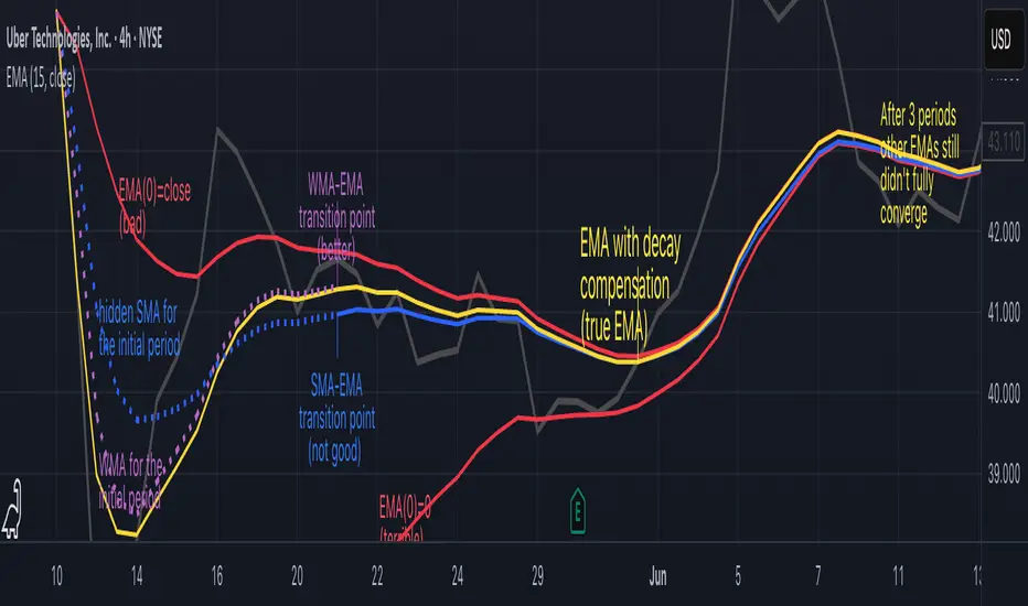
How do we calculate the first EMA value when there's no previous EMA available? Let's see some possible options used throughout the history:
Start with zero : EMA(0) = 0. This creates stupidly large distortion until enough bars pass for the horrible effect to diminish – like starting a trading account with zero balance but backdating a year of missed trades, then watching your balance struggle to climb out of a phantom debt for months.
Start with first price : EMA(0) = first price. This is better than starting with zero, but still causes initial distortion that will be extra-bad if the first price is an outlier – like forming your entire opinion of a stock based solely on its IPO day price, then wondering why your model is tanking for weeks afterward.
Use SMA for warmup : This is the tradition from the pencil-and-paper era of technical analysis – when calculators were luxury items and "algorithmic trading" meant your broker had neat handwriting. We first calculate an SMA over the initial period, then kickstart the EMA with this average value. It's widely used due to tradition, not merit, creating a mathematical Frankenstein that uses an FIR filter (SMA) during the initial period before abruptly switching to an IIR filter (EMA). This methodology is so aesthetically offensive (abrupt kink on the transition from SMA to EMA) that charting platforms hide these early values entirely, pretending EMA simply doesn't exist until the warmup period passes – the technical analysis equivalent of sweeping dust under the rug.
Use WMA for warmup : This one was never popular because it is harder to calculate with a pencil - compared to using simple SMA for warmup. Weighted Moving Average provides a much better approximation of a starting value as its linear descending profile is much closer to the EMA's decay profile.
These methods all share one problem: they produce inaccurate initial values that traders often hide or discard, much like how hedge funds conveniently report awesome performance "since strategy inception" only after their disastrous first quarter has been surgically removed from the track record.
▶️ A Better Way to start EMA: Decaying compensation
Think of it this way: An ideal EMA uses an infinite history of prices, but we only have data starting from a specific point. This creates a problem - our EMA starts with an incorrect assumption that all previous prices were all zero, all close, or all average – like trying to write someone's biography but only having information about their life since last Tuesday.
But there is a better way. It requires more than high school math comprehension and is more computationally intensive, but is mathematically correct and numerically stable. This approach involves compensating calculated EMA values for the "phantom data" that would have existed before our first price point.
Here's how phantom data compensation works:
We start our normal EMA calculation:
EMA_today = EMA_yesterday + α × (Price_today - EMA_yesterday)
But we add a correction factor that adjusts for the missing history:
Correction = 1 at the start
Correction = Correction × (1-α) after each calculation
We then apply this correction:
True_EMA = Raw_EMA / (1-Correction)
This correction factor starts at 1 (full compensation effect) and gets exponentially smaller with each new price bar. After enough data points, the correction becomes so small (i.e., below 0.0000000001) that we can stop applying it as it is no longer relevant.
Let's see how this works in practice:
For the first price bar:
Raw_EMA = 0
Correction = 1
True_EMA = Price (since 0 ÷ (1-1) is undefined, we use the first price)
For the second price bar:
Raw_EMA = α × (Price_2 - 0) + 0 = α × Price_2
Correction = 1 × (1-α) = (1-α)
True_EMA = α × Price_2 ÷ (1-(1-α)) = Price_2
For the third price bar:
Raw_EMA updates using the standard formula
Correction = (1-α) × (1-α) = (1-α)²
True_EMA = Raw_EMA ÷ (1-(1-α)²)
With each new price, the correction factor shrinks exponentially. After about -log₁₀(1e-10)/log₁₀(1-α) bars, the correction becomes negligible, and our EMA calculation matches what we would get if we had infinite historical data.
This approach provides accurate EMA values from the very first calculation. There's no need to use SMA for warmup or discard early values before output converges - EMA is mathematically correct from first value, ready to party without the awkward warmup phase.
Here is Pine Script 6 implementation of EMA that can take alpha parameter directly (or period if desired), returns valid values from the start, is resilient to dirty input values, uses decaying compensator instead of SMA, and uses the least amount of computational cycles possible.
// Enhanced EMA function with proper initialization and efficient calculation
ema(series float source, simple int period=0, simple float alpha=0)=>
// Input validation - one of alpha or period must be provided
if alpha<=0 and period<=0
runtime.error("Alpha or period must be provided")
// Calculate alpha from period if alpha not directly specified
float a = alpha > 0 ? alpha : 2.0 / math.max(period, 1)
// Initialize variables for EMA calculation
var float ema = na // Stores raw EMA value
var float result = na // Stores final corrected EMA
var float e = 1.0 // Decay compensation factor
var bool warmup = true // Flag for warmup phase
if not na(source)
if na(ema)
// First value case - initialize EMA to zero
// (we'll correct this immediately with the compensation)
ema := 0
result := source
else
// Standard EMA calculation (optimized formula)
ema := a * (source - ema) + ema
if warmup
// During warmup phase, apply decay compensation
e *= (1-a) // Update decay factor
float c = 1.0 / (1.0 - e) // Calculate correction multiplier
result := c * ema // Apply correction
// Stop warmup phase when correction becomes negligible
if e <= 1e-10
warmup := false
else
// After warmup, EMA operates without correction
result := ema
result // Return the properly compensated EMA value
▶️ CONCLUSION
EMA isn't just a "better SMA"—it is a fundamentally different tool, like how a submarine differs from a sailboat – both float, but the similarities end there. EMA responds to inputs differently, weighs historical data differently, and requires different initialization techniques.
By understanding these differences, traders can make more informed decisions about when and how to use EMA in trading strategies. And as EMA is embedded in so many other complex and compound indicators and strategies, if system uses tainted and inferior EMA calculatiomn, it is doing a disservice to all derivative indicators too – like building a skyscraper on a foundation of Jell-O.
The next time you add an EMA to your chart, remember: you're not just looking at a "faster moving average." You're using an INFINITE IMPULSE RESPONSE filter that carries the echo of all previous price actions, properly weighted to help make better trading decisions.
EMA done right might significantly improve the quality of all signals, strategies, and trades that rely on EMA somewhere deep in its algorithmic bowels – proving once again that math skills are indeed useful after high school, no matter what your guidance counselor told you.
Smart Money Flow Signals [QuantAlgo]🟢 Overview
The Smart Money Flow Signals indicator synthesizes significant volume-price dynamics through multi-component analysis to identify potential accumulation and distribution phases driven by substantial market participants. It combines Money Flow Index momentum, Chaikin Money Flow accumulation patterns, volume-weighted price momentum, and buying/selling pressure metrics into a unified composite oscillator that quantifies periods of concentrated capital movement, helping traders and investors identify conditions where significant volume participants may be actively positioning across multiple market conditions and timeframes.
🟢 How It Works
The indicator's core methodology lies in its weighted composite approach, where multiple volume-price components are calculated sequentially and then integrated to create a comprehensive significant flow activity signal.
First, the Money Flow Index (MFI) is calculated to measure buying and selling pressure by incorporating volume into price momentum analysis:
raw_money_flow = source * volume
positive_flow = source >= source ? raw_money_flow : 0
negative_flow = source < source ? raw_money_flow : 0
positive_money_flow = math.sum(positive_flow, mfi_period)
negative_money_flow = math.sum(negative_flow, mfi_period)
money_flow_index = 100 - 100 / (1 + positive_money_flow / negative_money_flow)
This creates an RSI-style momentum indicator that tracks whether money (price × volume) is flowing into or out of the asset, with values ranging from 0 to 100 where readings above 50 suggest buying pressure dominance.
Then, Chaikin Money Flow (CMF) is computed to evaluate accumulation and distribution by analyzing where prices close within each bar's range, weighted by volume:
money_flow_multiplier = high != low ? (close - low - (high - close)) / (high - low) : 0
money_flow_volume = money_flow_multiplier * volume
volume_sma = ta.sma(volume, trend_period)
chaikin_money_flow = volume_sma != 0 ? ta.sma(money_flow_volume, trend_period) / volume_sma : 0
Positive CMF values indicate accumulation (closes near the high of the range), while negative values indicate distribution (closes near the low of the range), with volume weighting emphasizing periods of significant participation.
Next, Volume Analysis is performed to quantify current volume intensity relative to historical averages:
volume_average = ta.sma(volume, trend_period)
volume_strength = volume_average != 0 ? volume / volume_average : 1
volume_weight = math.log(volume_strength + 1)
The logarithmic transformation creates a volume weight that amplifies signals during high-volume periods while preventing extreme volume spikes from overwhelming the composite calculation.
Following this, Buy/Sell Pressure is quantified by comparing cumulative volume during bullish versus bearish candles:
buying_pressure = math.sum(volume * (close >= open ? 1 : 0), trend_period)
selling_pressure = math.sum(volume * (close < open ? 1 : 0), trend_period)
pressure_ratio = (buying_pressure - selling_pressure) / (buying_pressure + selling_pressure) * 100
This creates a directional pressure ratio that reveals whether significant participants are predominantly buying or selling, expressed as a percentage between -100 (all selling) and +100 (all buying).
Then, Volume-Weighted Momentum is calculated through an exponential smoothing channel that adjusts price deviation based on volume intensity:
exponential_smooth_average = ta.ema(source, momentum_channel_period)
deviation = ta.ema(math.abs(source - exponential_smooth_average), momentum_channel_period)
channel_index = deviation != 0 ? (source - exponential_smooth_average) / (0.015 * deviation) * (1 + volume_weight * 0.5) : 0
This channel index measures how far price has deviated from its exponential average relative to typical deviation, with the volume weight multiplier (1 + volume_weight * 0.5) amplifying the signal when significant volume accompanies the price movement.
Finally, the Composite Wave is constructed by combining all components with specific weighting to create the final oscillator:
momentum_wave = ta.ema(channel_index, trend_period)
money_flow_wave = (money_flow_index - 50) * 1.2
chaikin_flow_wave = chaikin_money_flow * 100
composite_wave = momentum_wave * 0.5 + chaikin_flow_wave * 0.3 + money_flow_wave * 0.2
smoothed_wave = ta.sma(composite_wave, signal_smoothing)
This creates a multi-dimensional volume flow oscillator that combines price-volume momentum, accumulation-distribution patterns, and buying-selling pressure into a single signal, providing traders with probabilistic insights into periods of concentrated market activity and directional bias based on weighted component convergence.
🟢 Signal Interpretation
▶ Positive Values (Above Zero, Green): Composite money flow above equilibrium indicating net accumulation pressure, positive buying volume dominance, and bullish volume-price alignment = Favorable conditions for long positions, significant capital flowing into the asset = Buy/hold opportunities
▶ Negative Values (Below Zero, Red): Composite money flow below equilibrium indicating net distribution pressure, negative selling volume dominance, and bearish volume-price alignment = Unfavorable conditions for long positions, significant capital flowing out of the asset = Sell/short opportunities
▶ Extreme Overbought Zone: Excessive bullish money flow indicating potential accumulation exhaustion, where buying pressure may have reached unsustainable levels with elevated reversal risk = Caution on new longs, potential distribution phase beginning, profit-taking zone for existing positions
▶ Extreme Oversold Zone: Excessive bearish money flow indicating potential distribution exhaustion, where selling pressure may have reached unsustainable levels with elevated reversal risk = Caution on new shorts, potential accumulation phase beginning, buying opportunity zone for contrarian entries
▶ Smoothed Trend Line (White) Alignment: When the smoothed trend line confirms the composite wave direction, it validates the underlying volume-price trend and filters false signals caused by short-term noise
▶ Volume Intensity Correlation: Gradient intensity (color saturation) reflects combined wave strength, volume participation, and directional alignment, where darker/more saturated colors indicate stronger concentrated activity and higher-probability directional moves
🟢 Features
▶ Preconfigured Presets: Three optimized parameter configurations accommodate different trading styles, timeframes, and market analysis approaches.
1. "Default" provides balanced volume flow measurement suitable for swing trading on 4-hour and daily charts, offering moderate responsiveness to money flow shifts with standard RSI-equivalent MFI period and moderate smoothing for most market conditions.
2. "Fast Response" delivers heightened sensitivity optimized for active intraday trading and scalping on 1-minute to 1-hour charts, using compressed calculation periods across all components and minimal smoothing to capture rapid volume flow changes and quick trend shifts as they develop, ideal for early entry/exit opportunities with acceptance of increased signal frequency during consolidation.
3. "Smooth Trend" offers conservative extreme identification ideal for position trading and long-term analysis on daily to weekly charts, employing extended periods across all money flow components with substantial smoothing to filter short-term noise and isolate only strong, sustained accumulation and distribution phases driven by significant volume participants.
▶ Built-in Alerts: Seven alert conditions enable comprehensive automated monitoring of significant money flow transitions and extreme market states.
1. "Bullish Flow" triggers when the composite wave crosses above zero, signaling the shift from distribution to accumulation and concentrated buying activity beginning.
2. "Bearish Flow" activates when the composite wave crosses below zero, signaling the shift from accumulation to distribution and concentrated selling activity starting.
3. "Any Flow Direction Change" provides a combined notification for either bullish or bearish crossover regardless of direction, useful for general money flow momentum shifts.
4. "Extreme Overbought" alerts when the composite wave reaches or exceeds the overbought threshold (default +60), indicating excessive buying pressure and potential exhaustion.
5. "Extreme Oversold" notifies when the composite wave reaches or falls below the oversold threshold (default -60), indicating excessive selling pressure and potential capitulation.
6. "Overbought Reversal" triggers specifically when the wave crosses back down through the overbought level after being extended, signaling the beginning of distribution from extreme levels.
7. "Oversold Reversal" activates when the wave crosses back up through the oversold level after being extended, signaling the beginning of accumulation from extreme levels.
▶ Color Customization: Six visual themes (Classic, Aqua, Cosmic, Ember, Neon, plus Custom) accommodate different chart backgrounds and visual preferences, ensuring optimal contrast and immediate identification of bullish versus bearish volume flow conditions across various devices and screen sizes. Optional bar coloring provides instant visual context of current significant volume activity intensity and direction without switching between the price pane and indicator pane, enabling traders and investors to immediately assess volume-price positioning dynamics while analyzing price action.

Moving_AveragesLibrary "Moving_Averages"
This library contains majority important moving average functions with int series support. Which means that they can be used with variable length input. For conventional use, please use tradingview built-in ta functions for moving averages as they are more precise. I'll use functions in this library for my other scripts with dynamic length inputs.
ema(src, len)
Exponential Moving Average (EMA)
Parameters:
src : Source
len : Period
Returns: Exponential Moving Average with Series Int Support (EMA)
alma(src, len, a_offset, a_sigma)
Arnaud Legoux Moving Average (ALMA)
Parameters:
src : Source
len : Period
a_offset : Arnaud Legoux offset
a_sigma : Arnaud Legoux sigma
Returns: Arnaud Legoux Moving Average (ALMA)
covwema(src, len)
Coefficient of Variation Weighted Exponential Moving Average (COVWEMA)
Parameters:
src : Source
len : Period
Returns: Coefficient of Variation Weighted Exponential Moving Average (COVWEMA)
covwma(src, len)
Coefficient of Variation Weighted Moving Average (COVWMA)
Parameters:
src : Source
len : Period
Returns: Coefficient of Variation Weighted Moving Average (COVWMA)
dema(src, len)
DEMA - Double Exponential Moving Average
Parameters:
src : Source
len : Period
Returns: DEMA - Double Exponential Moving Average
edsma(src, len, ssfLength, ssfPoles)
EDSMA - Ehlers Deviation Scaled Moving Average
Parameters:
src : Source
len : Period
ssfLength : EDSMA - Super Smoother Filter Length
ssfPoles : EDSMA - Super Smoother Filter Poles
Returns: Ehlers Deviation Scaled Moving Average (EDSMA)
eframa(src, len, FC, SC)
Ehlrs Modified Fractal Adaptive Moving Average (EFRAMA)
Parameters:
src : Source
len : Period
FC : Lower Shift Limit for Ehlrs Modified Fractal Adaptive Moving Average
SC : Upper Shift Limit for Ehlrs Modified Fractal Adaptive Moving Average
Returns: Ehlrs Modified Fractal Adaptive Moving Average (EFRAMA)
ehma(src, len)
EHMA - Exponential Hull Moving Average
Parameters:
src : Source
len : Period
Returns: Exponential Hull Moving Average (EHMA)
etma(src, len)
Exponential Triangular Moving Average (ETMA)
Parameters:
src : Source
len : Period
Returns: Exponential Triangular Moving Average (ETMA)
frama(src, len)
Fractal Adaptive Moving Average (FRAMA)
Parameters:
src : Source
len : Period
Returns: Fractal Adaptive Moving Average (FRAMA)
hma(src, len)
HMA - Hull Moving Average
Parameters:
src : Source
len : Period
Returns: Hull Moving Average (HMA)
jma(src, len, jurik_phase, jurik_power)
Jurik Moving Average - JMA
Parameters:
src : Source
len : Period
jurik_phase : Jurik (JMA) Only - Phase
jurik_power : Jurik (JMA) Only - Power
Returns: Jurik Moving Average (JMA)
kama(src, len, k_fastLength, k_slowLength)
Kaufman's Adaptive Moving Average (KAMA)
Parameters:
src : Source
len : Period
k_fastLength : Number of periods for the fastest exponential moving average
k_slowLength : Number of periods for the slowest exponential moving average
Returns: Kaufman's Adaptive Moving Average (KAMA)
kijun(_high, _low, len, kidiv)
Kijun v2
Parameters:
_high : High value of bar
_low : Low value of bar
len : Period
kidiv : Kijun MOD Divider
Returns: Kijun v2
lsma(src, len, offset)
LSMA/LRC - Least Squares Moving Average / Linear Regression Curve
Parameters:
src : Source
len : Period
offset : Offset
Returns: Least Squares Moving Average (LSMA)/ Linear Regression Curve (LRC)
mf(src, len, beta, feedback, z)
MF - Modular Filter
Parameters:
src : Source
len : Period
beta : Modular Filter, General Filter Only - Beta
feedback : Modular Filter Only - Feedback
z : Modular Filter Only - Feedback Weighting
Returns: Modular Filter (MF)
rma(src, len)
RMA - RSI Moving average
Parameters:
src : Source
len : Period
Returns: RSI Moving average (RMA)
sma(src, len)
SMA - Simple Moving Average
Parameters:
src : Source
len : Period
Returns: Simple Moving Average (SMA)
smma(src, len)
Smoothed Moving Average (SMMA)
Parameters:
src : Source
len : Period
Returns: Smoothed Moving Average (SMMA)
stma(src, len)
Simple Triangular Moving Average (STMA)
Parameters:
src : Source
len : Period
Returns: Simple Triangular Moving Average (STMA)
tema(src, len)
TEMA - Triple Exponential Moving Average
Parameters:
src : Source
len : Period
Returns: Triple Exponential Moving Average (TEMA)
thma(src, len)
THMA - Triple Hull Moving Average
Parameters:
src : Source
len : Period
Returns: Triple Hull Moving Average (THMA)
vama(src, len, volatility_lookback)
VAMA - Volatility Adjusted Moving Average
Parameters:
src : Source
len : Period
volatility_lookback : Volatility lookback length
Returns: Volatility Adjusted Moving Average (VAMA)
vidya(src, len)
Variable Index Dynamic Average (VIDYA)
Parameters:
src : Source
len : Period
Returns: Variable Index Dynamic Average (VIDYA)
vwma(src, len)
Volume-Weighted Moving Average (VWMA)
Parameters:
src : Source
len : Period
Returns: Volume-Weighted Moving Average (VWMA)
wma(src, len)
WMA - Weighted Moving Average
Parameters:
src : Source
len : Period
Returns: Weighted Moving Average (WMA)
zema(src, len)
Zero-Lag Exponential Moving Average (ZEMA)
Parameters:
src : Source
len : Period
Returns: Zero-Lag Exponential Moving Average (ZEMA)
zsma(src, len)
Zero-Lag Simple Moving Average (ZSMA)
Parameters:
src : Source
len : Period
Returns: Zero-Lag Simple Moving Average (ZSMA)
evwma(src, len)
EVWMA - Elastic Volume Weighted Moving Average
Parameters:
src : Source
len : Period
Returns: Elastic Volume Weighted Moving Average (EVWMA)
tt3(src, len, a1_t3)
Tillson T3
Parameters:
src : Source
len : Period
a1_t3 : Tillson T3 Volume Factor
Returns: Tillson T3
gma(src, len)
GMA - Geometric Moving Average
Parameters:
src : Source
len : Period
Returns: Geometric Moving Average (GMA)
wwma(src, len)
WWMA - Welles Wilder Moving Average
Parameters:
src : Source
len : Period
Returns: Welles Wilder Moving Average (WWMA)
ama(src, _high, _low, len, ama_f_length, ama_s_length)
AMA - Adjusted Moving Average
Parameters:
src : Source
_high : High value of bar
_low : Low value of bar
len : Period
ama_f_length : Fast EMA Length
ama_s_length : Slow EMA Length
Returns: Adjusted Moving Average (AMA)
cma(src, len)
Corrective Moving average (CMA)
Parameters:
src : Source
len : Period
Returns: Corrective Moving average (CMA)
gmma(src, len)
Geometric Mean Moving Average (GMMA)
Parameters:
src : Source
len : Period
Returns: Geometric Mean Moving Average (GMMA)
ealf(src, len, LAPercLen_, FPerc_)
Ehler's Adaptive Laguerre filter (EALF)
Parameters:
src : Source
len : Period
LAPercLen_ : Median Length
FPerc_ : Median Percentage
Returns: Ehler's Adaptive Laguerre filter (EALF)
elf(src, len, LAPercLen_, FPerc_)
ELF - Ehler's Laguerre filter
Parameters:
src : Source
len : Period
LAPercLen_ : Median Length
FPerc_ : Median Percentage
Returns: Ehler's Laguerre Filter (ELF)
edma(src, len)
Exponentially Deviating Moving Average (MZ EDMA)
Parameters:
src : Source
len : Period
Returns: Exponentially Deviating Moving Average (MZ EDMA)
pnr(src, len, rank_inter_Perc_)
PNR - percentile nearest rank
Parameters:
src : Source
len : Period
rank_inter_Perc_ : Rank and Interpolation Percentage
Returns: Percentile Nearest Rank (PNR)
pli(src, len, rank_inter_Perc_)
PLI - Percentile Linear Interpolation
Parameters:
src : Source
len : Period
rank_inter_Perc_ : Rank and Interpolation Percentage
Returns: Percentile Linear Interpolation (PLI)
rema(src, len)
Range EMA (REMA)
Parameters:
src : Source
len : Period
Returns: Range EMA (REMA)
sw_ma(src, len)
Sine-Weighted Moving Average (SW-MA)
Parameters:
src : Source
len : Period
Returns: Sine-Weighted Moving Average (SW-MA)
vwap(src, len)
Volume Weighted Average Price (VWAP)
Parameters:
src : Source
len : Period
Returns: Volume Weighted Average Price (VWAP)
mama(src, len)
MAMA - MESA Adaptive Moving Average
Parameters:
src : Source
len : Period
Returns: MESA Adaptive Moving Average (MAMA)
fama(src, len)
FAMA - Following Adaptive Moving Average
Parameters:
src : Source
len : Period
Returns: Following Adaptive Moving Average (FAMA)
hkama(src, len)
HKAMA - Hilbert based Kaufman's Adaptive Moving Average
Parameters:
src : Source
len : Period
Returns: Hilbert based Kaufman's Adaptive Moving Average (HKAMA)
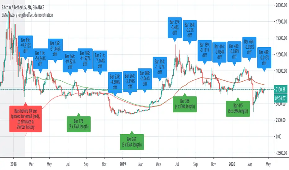
Demonstration of how history length affects all EMA valuesI saw some discussion of this so I whipped up an example to prove the that effect of history length on EMA values is pronounced, even for bars much further than the EMA length from the first candle of the chart.
This chart has two 89-bar EMAs of the close: a green one and a red one. However, for the red one, the first 89 bars of the graph are considered to have a close of "0", which is exactly whatTradingView's EMA calculation uses for bars before the start of the graph.
This is because unlike other moving averages, which reference the price of previous bars, the EMA references the EMA of previous bars. Therefore, bars closer to the beginning of the chart, where TradingView can't calculate an EMA because there is no previous EMA and therefore uses 0, will return substantially different values for the EMA() function that the same cart would with more history.
The further a bar is back in history, the less influence it has. However, every single historical bar has some influence on the EMA of every later bar.
To allow you to see this for yourself, this script contains the following inputs which you can change to see the effect:
-EMA period (default 89)
-Number of bars to ignore for EMA2 (default 89)
-decimal precision to show differences in. By making this a large number you can see that, although the effects diminish, history length affects all EMA values for the char.
-label spacing (increase this if you have a long history and run into TV's 50-label limit)
Multiple EMAMultiple EMA. Color switch of slowest EMA (def=200) when price close below or above. Trend marker when fastest EMA (def=9) cross slowest EMA (def=200).
Multiple EMAMultiple EMA lines. Color switch of slowest EMA (def=200) when price close above or below. Trend marker when fastest EMA (def=9) cross slowest one.

Mean Reversion Cloud (Ornstein-Uhlenbeck) // AlgoFyreThe Mean Reversion Cloud (Ornstein-Uhlenbeck) indicator detects mean-reversion opportunities by applying the Ornstein-Uhlenbeck process. It calculates a dynamic mean using an Exponential Weighted Moving Average, surrounded by volatility bands, signaling potential buy/sell points when prices deviate.
TABLE OF CONTENTS
🔶 ORIGINALITY
🔸Adaptive Mean Calculation
🔸Volatility-Based Cloud
🔸Speed of Reversion (θ)
🔶 FUNCTIONALITY
🔸Dynamic Mean and Volatility Bands
🞘 How it works
🞘 How to calculate
🞘 Code extract
🔸Visualization via Table and Plotshapes
🞘 Table Overview
🞘 Plotshapes Explanation
🞘 Code extract
🔶 INSTRUCTIONS
🔸Step-by-Step Guidelines
🞘 Setting Up the Indicator
🞘 Understanding What to Look For on the Chart
🞘 Possible Entry Signals
🞘 Possible Take Profit Strategies
🞘 Possible Stop-Loss Levels
🞘 Additional Tips
🔸Customize settings
🔶 CONCLUSION
▅▅▅▅▅▅▅▅▅▅▅▅▅▅▅▅▅▅▅▅▅▅▅▅▅▅▅▅▅▅▅▅▅▅▅▅▅▅▅▅▅▅▅▅▅▅
🔶 ORIGINALITY The Mean Reversion Cloud (Ornstein-Uhlenbeck) is a unique indicator that applies the Ornstein-Uhlenbeck stochastic process to identify mean-reverting behavior in asset prices. Unlike traditional moving average-based indicators, this model uses an Exponentially Weighted Moving Average (EWMA) to calculate the long-term mean, dynamically adjusting to recent price movements while still considering all historical data. It also incorporates volatility bands, providing a "cloud" that visually highlights overbought or oversold conditions. By calculating the speed of mean reversion (θ) through the autocorrelation of log returns, this indicator offers traders a more nuanced and mathematically robust tool for identifying mean-reversion opportunities. These innovations make it especially useful for markets that exhibit range-bound characteristics, offering timely buy and sell signals based on statistical deviations from the mean.
🔸Adaptive Mean Calculation Traditional MA indicators use fixed lengths, which can lead to lagging signals or over-sensitivity in volatile markets. The Mean Reversion Cloud uses an Exponentially Weighted Moving Average (EWMA), which adapts to price movements by dynamically adjusting its calculation, offering a more responsive mean.
🔸Volatility-Based Cloud Unlike simple moving averages that only plot a single line, the Mean Reversion Cloud surrounds the dynamic mean with volatility bands. These bands, based on standard deviations, provide traders with a visual cue of when prices are statistically likely to revert, highlighting potential reversal zones.
🔸Speed of Reversion (θ) The indicator goes beyond price averages by calculating the speed at which the price reverts to the mean (θ), using the autocorrelation of log returns. This gives traders an additional tool for estimating the likelihood and timing of mean reversion, making the signals more reliable in practice.
🔶 FUNCTIONALITY The Mean Reversion Cloud (Ornstein-Uhlenbeck) indicator is designed to detect potential mean-reversion opportunities in asset prices by applying the Ornstein-Uhlenbeck stochastic process. It calculates a dynamic mean through the Exponentially Weighted Moving Average (EWMA) and plots volatility bands based on the standard deviation of the asset's price over a specified period. These bands create a "cloud" that represents expected price fluctuations, helping traders to identify overbought or oversold conditions. By calculating the speed of reversion (θ) from the autocorrelation of log returns, the indicator offers a more refined way of assessing how quickly prices may revert to the mean. Additionally, the inclusion of volatility provides a comprehensive view of market conditions, allowing for more accurate buy and sell signals.
Let's dive into the details:
🔸Dynamic Mean and Volatility Bands The dynamic mean (μ) is calculated using the EWMA, giving more weight to recent prices but considering all historical data. This process closely resembles the Ornstein-Uhlenbeck (OU) process, which models the tendency of a stochastic variable (such as price) to revert to its mean over time. Volatility bands are plotted around the mean using standard deviation, forming the "cloud" that signals overbought or oversold conditions. The cloud adapts dynamically to price fluctuations and market volatility, making it a versatile tool for mean-reversion strategies. 🞘 How it works Step one: Calculate the dynamic mean (μ) The Ornstein-Uhlenbeck process describes how a variable, such as an asset's price, tends to revert to a long-term mean while subject to random fluctuations. In this indicator, the EWMA is used to compute the dynamic mean (μ), mimicking the mean-reverting behavior of the OU process. Use the EWMA formula to compute a weighted mean that adjusts to recent price movements. Assign exponentially decreasing weights to older data while giving more emphasis to current prices. Step two: Plot volatility bands Calculate the standard deviation of the price over a user-defined period to determine market volatility. Position the upper and lower bands around the mean by adding and subtracting a multiple of the standard deviation. 🞘 How to calculate Exponential Weighted Moving Average (EWMA)
The EWMA dynamically adjusts to recent price movements:
mu_t = lambda * mu_{t-1} + (1 - lambda) * P_t
Where mu_t is the mean at time t, lambda is the decay factor, and P_t is the price at time t. The higher the decay factor, the more weight is given to recent data.
Autocorrelation (ρ) and Standard Deviation (σ)
To measure mean reversion speed and volatility: rho = correlation(log(close), log(close ), length) Where rho is the autocorrelation of log returns over a specified period.
To calculate volatility:
sigma = stdev(close, length)
Where sigma is the standard deviation of the asset's closing price over a specified length.
Upper and Lower Bands
The upper and lower bands are calculated as follows:
upper_band = mu + (threshold * sigma)
lower_band = mu - (threshold * sigma)
Where threshold is a multiplier for the standard deviation, usually set to 2. These bands represent the range within which the price is expected to fluctuate, based on current volatility and the mean.
🞘 Code extract // Calculate Returns
returns = math.log(close / close )
// Calculate Long-Term Mean (μ) using EWMA over the entire dataset
var float ewma_mu = na // Initialize ewma_mu as 'na'
ewma_mu := na(ewma_mu ) ? close : decay_factor * ewma_mu + (1 - decay_factor) * close
mu = ewma_mu
// Calculate Autocorrelation at Lag 1
rho1 = ta.correlation(returns, returns , corr_length)
// Ensure rho1 is within valid range to avoid errors
rho1 := na(rho1) or rho1 <= 0 ? 0.0001 : rho1
// Calculate Speed of Mean Reversion (θ)
theta = -math.log(rho1)
// Calculate Volatility (σ)
sigma = ta.stdev(close, corr_length)
// Calculate Upper and Lower Bands
upper_band = mu + threshold * sigma
lower_band = mu - threshold * sigma
🔸Visualization via Table and Plotshapes
The table shows key statistics such as the current value of the dynamic mean (μ), the number of times the price has crossed the upper or lower bands, and the consecutive number of bars that the price has remained in an overbought or oversold state.
Plotshapes (diamonds) are used to signal buy and sell opportunities. A green diamond below the price suggests a buy signal when the price crosses below the lower band, and a red diamond above the price indicates a sell signal when the price crosses above the upper band.
The table and plotshapes provide a comprehensive visualization, combining both statistical and actionable information to aid decision-making.
🞘 Code extract // Reset consecutive_bars when price crosses the mean
var consecutive_bars = 0
if (close < mu and close >= mu) or (close > mu and close <= mu)
consecutive_bars := 0
else if math.abs(deviation) > 0
consecutive_bars := math.min(consecutive_bars + 1, dev_length)
transparency = math.max(0, math.min(100, 100 - (consecutive_bars * 100 / dev_length)))
🔶 INSTRUCTIONS
The Mean Reversion Cloud (Ornstein-Uhlenbeck) indicator can be set up by adding it to your TradingView chart and configuring parameters such as the decay factor, autocorrelation length, and volatility threshold to suit current market conditions. Look for price crossovers and deviations from the calculated mean for potential entry signals. Use the upper and lower bands as dynamic support/resistance levels for setting take profit and stop-loss orders. Combining this indicator with additional trend-following or momentum-based indicators can improve signal accuracy. Adjust settings for better mean-reversion detection and risk management.
🔸Step-by-Step Guidelines
🞘 Setting Up the Indicator
Adding the Indicator to the Chart:
Go to your TradingView chart.
Click on the "Indicators" button at the top.
Search for "Mean Reversion Cloud (Ornstein-Uhlenbeck)" in the indicators list.
Click on the indicator to add it to your chart.
Configuring the Indicator:
Open the indicator settings by clicking on the gear icon next to its name on the chart.
Decay Factor: Adjust the decay factor (λ) to control the responsiveness of the mean calculation. A higher value prioritizes recent data.
Autocorrelation Length: Set the autocorrelation length (θ) for calculating the speed of mean reversion. Longer lengths consider more historical data.
Threshold: Define the number of standard deviations for the upper and lower bands to determine how far price must deviate to trigger a signal.
Chart Setup:
Select the appropriate timeframe (e.g., 1-hour, daily) based on your trading strategy.
Consider using other indicators such as RSI or MACD to confirm buy and sell signals.
🞘 Understanding What to Look For on the Chart
Indicator Behavior:
Observe how the price interacts with the dynamic mean and volatility bands. The price staying within the bands suggests mean-reverting behavior, while crossing the bands signals potential entry points.
The indicator calculates overbought/oversold conditions based on deviation from the mean, highlighted by color-coded cloud areas on the chart.
Crossovers and Deviation:
Look for crossovers between the price and the mean (μ) or the bands. A bullish crossover occurs when the price crosses below the lower band, signaling a potential buying opportunity.
A bearish crossover occurs when the price crosses above the upper band, suggesting a potential sell signal.
Deviations from the mean indicate market extremes. A large deviation indicates that the price is far from the mean, suggesting a potential reversal.
Slope and Direction:
Pay attention to the slope of the mean (μ). A rising slope suggests bullish market conditions, while a declining slope signals a bearish market.
The steepness of the slope can indicate the strength of the mean-reversion trend.
🞘 Possible Entry Signals
Bullish Entry:
Crossover Entry: Enter a long position when the price crosses below the lower band with a positive deviation from the mean.
Confirmation Entry: Use additional indicators like RSI (above 50) or increasing volume to confirm the bullish signal.
Bearish Entry:
Crossover Entry: Enter a short position when the price crosses above the upper band with a negative deviation from the mean.
Confirmation Entry: Look for RSI (below 50) or decreasing volume to confirm the bearish signal.
Deviation Confirmation:
Enter trades when the deviation from the mean is significant, indicating that the price has strayed far from its expected value and is likely to revert.
🞘 Possible Take Profit Strategies
Static Take Profit Levels:
Set predefined take profit levels based on historical volatility, using the upper and lower bands as guides.
Place take profit orders near recent support/resistance levels, ensuring you're capitalizing on the mean-reversion behavior.
Trailing Stop Loss:
Use a trailing stop based on a percentage of the price deviation from the mean to lock in profits as the trend progresses.
Adjust the trailing stop dynamically along the calculated bands to protect profits as the price returns to the mean.
Deviation-Based Exits:
Exit when the deviation from the mean starts to decrease, signaling that the price is returning to its equilibrium.
🞘 Possible Stop-Loss Levels
Initial Stop Loss:
Place an initial stop loss outside the lower band (for long positions) or above the upper band (for short positions) to protect against excessive deviations.
Use a volatility-based buffer to avoid getting stopped out during normal price fluctuations.
Dynamic Stop Loss:
Move the stop loss closer to the mean as the price converges back towards equilibrium, reducing risk.
Adjust the stop loss dynamically along the bands to account for sudden market movements.
🞘 Additional Tips
Combine with Other Indicators:
Enhance your strategy by combining the Mean Reversion Cloud with momentum indicators like MACD, RSI, or Bollinger Bands to confirm market conditions.
Backtesting and Practice:
Backtest the indicator on historical data to understand how it performs in various market environments.
Practice using the indicator on a demo account before implementing it in live trading.
Market Awareness:
Keep an eye on market news and events that might cause extreme price movements. The indicator reacts to price data and might not account for news-driven events that can cause large deviations.
🔸Customize settings 🞘 Decay Factor (λ): Defines the weight assigned to recent price data in the calculation of the mean. A value closer to 1 places more emphasis on recent prices, while lower values create a smoother, more lagging mean.
🞘 Autocorrelation Length (θ): Sets the period for calculating the speed of mean reversion and volatility. Longer lengths capture more historical data, providing smoother calculations, while shorter lengths make the indicator more responsive.
🞘 Threshold (σ): Specifies the number of standard deviations used to create the upper and lower bands. Higher thresholds widen the bands, producing fewer signals, while lower thresholds tighten the bands for more frequent signals.
🞘 Max Gradient Length (γ): Determines the maximum number of consecutive bars for calculating the deviation gradient. This setting impacts the transparency of the plotted bands based on the length of deviation from the mean.
🔶 CONCLUSION
The Mean Reversion Cloud (Ornstein-Uhlenbeck) indicator offers a sophisticated approach to identifying mean-reversion opportunities by applying the Ornstein-Uhlenbeck stochastic process. This dynamic indicator calculates a responsive mean using an Exponentially Weighted Moving Average (EWMA) and plots volatility-based bands to highlight overbought and oversold conditions. By incorporating advanced statistical measures like autocorrelation and standard deviation, traders can better assess market extremes and potential reversals. The indicator’s ability to adapt to price behavior makes it a versatile tool for traders focused on both short-term price deviations and longer-term mean-reversion strategies. With its unique blend of statistical rigor and visual clarity, the Mean Reversion Cloud provides an invaluable tool for understanding and capitalizing on market inefficiencies.
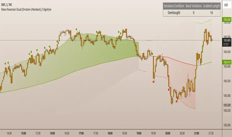
Moving Averages ProxyLibrary "MovingAveragesProxy"
Moving Averages Proxy - Library of all moving averages spread out in different libraries
rvwap(_src, fixedTfInput, minsInput, hoursInput, daysInput, minBarsInput)
Calculates the Rolling VWAP (customized VWAP developed by the team of TradingView)
Parameters:
_src : (float) Source. Default: close
fixedTfInput : (bool) Use a fixed time period. Default: false
minsInput : (int) Minutes. Default: 0
hoursInput : (int) Hours. Default: 0
daysInput : (int) Days. Default: 1
minBarsInput : (int) Bars. Default: 10
Returns: (float) Rolling VWAP
correlationMa(src, len, factor)
Correlation Moving Average
Parameters:
src : (float) Source. Default: close
len : (int) Length
factor : (float) Factor. Default: 1.7
Returns: (float) Correlation Moving Average
regma(src, len, lambda)
Regularized Exponential Moving Average
Parameters:
src : (float) Source. Default: close
len : (int) Length
lambda : (float) Lambda. Default: 0.5
Returns: (float) Regularized Exponential Moving Average
repma(src, len)
Repulsion Moving Average
Parameters:
src : (float) Source. Default: close
len : (int) Length
Returns: (float) Repulsion Moving Average
epma(src, length, offset)
End Point Moving Average
Parameters:
src : (float) Source. Default: close
length : (int) Length
offset : (float) Offset. Default: 4
Returns: (float) End Point Moving Average
lc_lsma(src, length)
1LC-LSMA (1 line code lsma with 3 functions)
Parameters:
src : (float) Source. Default: close
length : (int) Length
Returns: (float) 1LC-LSMA Moving Average
aarma(src, length)
Adaptive Autonomous Recursive Moving Average
Parameters:
src : (float) Source. Default: close
length : (int) Length
Returns: (float) Adaptive Autonomous Recursive Moving Average
alsma(src, length)
Adaptive Least Squares
Parameters:
src : (float) Source. Default: close
length : (int) Length
Returns: (float) Adaptive Least Squares
ahma(src, length)
Ahrens Moving Average
Parameters:
src : (float) Source. Default: close
length : (int) Length
Returns: (float) Ahrens Moving Average
adema(src)
Ahrens Moving Average
Parameters:
src : (float) Source. Default: close
Returns: (float) Moving Average
autol(src, lenDev)
Auto-Line
Parameters:
src : (float) Source. Default: close
lenDev : (int) Length for standard deviation
Returns: (float) Auto-Line
fibowma(src, length)
Fibonacci Weighted Moving Average
Parameters:
src : (float) Source. Default: close
length : (int) Length
Returns: (float) Moving Average
fisherlsma(src, length)
Fisher Least Squares Moving Average
Parameters:
src : (float) Source. Default: close
length : (int) Length
Returns: (float) Moving Average
leoma(src, length)
Leo Moving Average
Parameters:
src : (float) Source. Default: close
length : (int) Length
Returns: (float) Moving Average
linwma(src, period, weight)
Linear Weighted Moving Average
Parameters:
src : (float) Source. Default: close
period : (int) Length
weight : (int) Weight
Returns: (float) Moving Average
mcma(src, length)
McNicholl Moving Average
Parameters:
src : (float) Source. Default: close
length : (int) Length
Returns: (float) Moving Average
srwma(src, length)
Square Root Weighted Moving Average
Parameters:
src : (float) Source. Default: close
length : (int) Length
Returns: (float) Moving Average
EDSMA(src, len)
Ehlers Dynamic Smoothed Moving Average.
Parameters:
src : Series to use ('close' is used if no argument is supplied).
len : Lookback length to use.
Returns: EDSMA smoothing.
dema(x, t)
Double Exponential Moving Average.
Parameters:
x : Series to use ('close' is used if no argument is supplied).
t : Lookback length to use.
Returns: DEMA smoothing.
tema(src, len)
Triple Exponential Moving Average.
Parameters:
src : Series to use ('close' is used if no argument is supplied).
len : Lookback length to use.
Returns: TEMA smoothing.
smma(src, len)
Smoothed Moving Average.
Parameters:
src : Series to use ('close' is used if no argument is supplied).
len : Lookback length to use.
Returns: SMMA smoothing.
hullma(src, len)
Hull Moving Average.
Parameters:
src : Series to use ('close' is used if no argument is supplied).
len : Lookback length to use.
Returns: Hull smoothing.
frama(x, t)
Fractal Reactive Moving Average.
Parameters:
x : Series to use ('close' is used if no argument is supplied).
t : Lookback length to use.
Returns: FRAMA smoothing.
kama(x, t)
Kaufman's Adaptive Moving Average.
Parameters:
x : Series to use ('close' is used if no argument is supplied).
t : Lookback length to use.
Returns: KAMA smoothing.
vama(src, len)
Volatility Adjusted Moving Average.
Parameters:
src : Series to use ('close' is used if no argument is supplied).
len : Lookback length to use.
Returns: VAMA smoothing.
donchian(len)
Donchian Calculation.
Parameters:
len : Lookback length to use.
Returns: Average of the highest price and the lowest price for the specified look-back period.
Jurik(src, len)
Jurik Moving Average.
Parameters:
src : Series to use ('close' is used if no argument is supplied).
len : Lookback length to use.
Returns: JMA smoothing.
xema(src, len)
Optimized Exponential Moving Average.
Parameters:
src : Series to use ('close' is used if no argument is supplied).
len : Lookback length to use.
Returns: XEMA smoothing.
ehma(src, len)
EHMA - Exponential Hull Moving Average
Parameters:
src : Source
len : Period
Returns: Exponential Hull Moving Average (EHMA)
covwema(src, len)
Coefficient of Variation Weighted Exponential Moving Average (COVWEMA)
Parameters:
src : Source
len : Period
Returns: Coefficient of Variation Weighted Exponential Moving Average (COVWEMA)
covwma(src, len)
Coefficient of Variation Weighted Moving Average (COVWMA)
Parameters:
src : Source
len : Period
Returns: Coefficient of Variation Weighted Moving Average (COVWMA)
eframa(src, len, FC, SC)
Ehlrs Modified Fractal Adaptive Moving Average (EFRAMA)
Parameters:
src : Source
len : Period
FC : Lower Shift Limit for Ehlrs Modified Fractal Adaptive Moving Average
SC : Upper Shift Limit for Ehlrs Modified Fractal Adaptive Moving Average
Returns: Ehlrs Modified Fractal Adaptive Moving Average (EFRAMA)
etma(src, len)
Exponential Triangular Moving Average (ETMA)
Parameters:
src : Source
len : Period
Returns: Exponential Triangular Moving Average (ETMA)
rma(src, len)
RMA - RSI Moving average
Parameters:
src : Source
len : Period
Returns: RSI Moving average (RMA)
thma(src, len)
THMA - Triple Hull Moving Average
Parameters:
src : Source
len : Period
Returns: Triple Hull Moving Average (THMA)
vidya(src, len)
Variable Index Dynamic Average (VIDYA)
Parameters:
src : Source
len : Period
Returns: Variable Index Dynamic Average (VIDYA)
zsma(src, len)
Zero-Lag Simple Moving Average (ZSMA)
Parameters:
src : Source
len : Period
Returns: Zero-Lag Simple Moving Average (ZSMA)
zema(src, len)
Zero-Lag Exponential Moving Average (ZEMA)
Parameters:
src : Source
len : Period
Returns: Zero-Lag Exponential Moving Average (ZEMA)
evwma(src, len)
EVWMA - Elastic Volume Weighted Moving Average
Parameters:
src : Source
len : Period
Returns: Elastic Volume Weighted Moving Average (EVWMA)
tt3(src, len, a1_t3)
Tillson T3
Parameters:
src : Source
len : Period
a1_t3 : Tillson T3 Volume Factor
Returns: Tillson T3
gma(src, len)
GMA - Geometric Moving Average
Parameters:
src : Source
len : Period
Returns: Geometric Moving Average (GMA)
wwma(src, len)
WWMA - Welles Wilder Moving Average
Parameters:
src : Source
len : Period
Returns: Welles Wilder Moving Average (WWMA)
cma(src, len)
Corrective Moving average (CMA)
Parameters:
src : Source
len : Period
Returns: Corrective Moving average (CMA)
edma(src, len)
Exponentially Deviating Moving Average (MZ EDMA)
Parameters:
src : Source
len : Period
Returns: Exponentially Deviating Moving Average (MZ EDMA)
rema(src, len)
Range EMA (REMA)
Parameters:
src : Source
len : Period
Returns: Range EMA (REMA)
sw_ma(src, len)
Sine-Weighted Moving Average (SW-MA)
Parameters:
src : Source
len : Period
Returns: Sine-Weighted Moving Average (SW-MA)
mama(src, len)
MAMA - MESA Adaptive Moving Average
Parameters:
src : Source
len : Period
Returns: MESA Adaptive Moving Average (MAMA)
fama(src, len)
FAMA - Following Adaptive Moving Average
Parameters:
src : Source
len : Period
Returns: Following Adaptive Moving Average (FAMA)
hkama(src, len)
HKAMA - Hilbert based Kaufman's Adaptive Moving Average
Parameters:
src : Source
len : Period
Returns: Hilbert based Kaufman's Adaptive Moving Average (HKAMA)
getMovingAverage(type, src, len, lsmaOffset, inputAlmaOffset, inputAlmaSigma, FC, SC, a1_t3, fixedTfInput, daysInput, hoursInput, minsInput, minBarsInput, lambda, volumeWeighted, gamma_aarma, smooth, linweight, volatility_lookback, jurik_phase, jurik_power)
Abstract proxy function that invokes the calculation of a moving average according to type
Parameters:
type : (string) Type of moving average
src : (float) Source of series (close, high, low, etc.)
len : (int) Period of loopback to calculate the average
lsmaOffset : (int) Offset for Least Squares MA
inputAlmaOffset : (float) Offset for ALMA
inputAlmaSigma : (float) Sigma for ALMA
FC : (int) Lower Shift Limit for Ehlrs Modified Fractal Adaptive Moving Average
SC : (int) Upper Shift Limit for Ehlrs Modified Fractal Adaptive Moving Average
a1_t3 : (float) Tillson T3 Volume Factor
fixedTfInput : (bool) Use a fixed time period in Rolling VWAP
daysInput : (int) Days in Rolling VWAP
hoursInput : (int) Hours in Rolling VWAP
minsInput : (int) Minutrs in Rolling VWAP
minBarsInput : (int) Bars in Rolling VWAP
lambda : (float) Regularization Constant in Regularized EMA
volumeWeighted : (bool) Apply volume weighted calculation in selected moving average
gamma_aarma : (float) Gamma for Adaptive Autonomous Recursive Moving Average
smooth : (float) Smooth for Adaptive Least Squares
linweight : (float) Weight for Volume Weighted Moving Average
volatility_lookback : (int) Loopback for Volatility Adjusted Moving Average
jurik_phase : (int) Phase for Jurik Moving Average
jurik_power : (int) Power for Jurik Moving Average
Returns: (float) Moving average
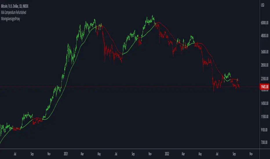
Volatility Signal-to-Noise Ratio🙏🏻 this is VSNR: the most effective and simple volatility regime detector & automatic volatility threshold scaler that somehow no1 ever talks about.
This is simply an inverse of the coefficient of variation of absolute returns, but properly constructed taking into account temporal information, and made online via recursive math with algocomplexity O(1) both in expanding and moving windows modes.
How do the available alternatives differ (while some’re just worse)?
Mainstream quant stat tests like Durbin-Watson, Dickey-Fuller etc: default implementations are ALL not time aware. They measure different kinds of regime, which is less (if at all) relevant for actual trading context. Mix of different math, high algocomplexity.
The closest one is MMI by financialhacker, but his approach is also not time aware, and has a higher algocomplexity anyways. Best alternative to mine, but pls modify it to use a time-weighted median.
Fractal dimension & its derivatives by John Ehlers: again not time aware, very low info gain, relies on bar sizes (high and lows), which don’t always exist unlike changes between datapoints. But it’s a geometric tool in essence, so this is fundamental. Let it watch your back if you already use it.
Hurst exponent: much higher algocomplexity, mix of parametric and non-parametric math inside. An invention, not a math entity. Again, not time aware. Also measures different kinds of regime.
How to set it up:
Given my other tools, I choose length so that it will match the amount of data that your trading method or study uses multiplied by ~ 4-5. E.g if you use some kind of bands to trade volatility and you calculate them over moving window 64, put VSNR on 256.
However it depends mathematically on many things, so for your methods you may instead need multipliers of 1 or ~ 16.
Additionally if you wanna use all data to estimate SNR, put 0 into length input.
How to use for regime detection:
First we define:
MR bias: mean reversion bias meaning volatility shorts would work better, fading levels would work better
Momo bias: momentum bias meaning volatility longs would work better, trading breakouts of levels would work better.
The study plots 3 horizontal thresholds for VSNR, just check its location:
Above upper level: significant Momo bias
Above 1 : Momo bias
Below 1 : MR bias
Below lower level: significant MR bias
Take a look at the screenshots, 2 completely different volatility regimes are spotted by VSNR, while an ADF does not show different regime:
^^ CBOT:ZN1!
^^ INDEX:BTCUSD
How to use as automatic volatility threshold scaler
Copy the code from the script, and use VSNR as a multiplier for your volatility threshold.
E.g you use a regression channel and fade/push upper and lower thresholds which are RMSEs multiples. Inside the code, multiply RMSE by VSNR, now you’re adaptive.
^^ The same logic as when MM bots widen spreads with vola goes wild.
How it works:
Returns follow Laplace distro -> logically abs returns follow exponential distro , cuz laplace = double exponential.
Exponential distro has a natural coefficient of variation = 1 -> signal to noise ratio defined as mean/stdev = 1 as well. The same can be said for Student t distro with parameter v = 4. So 1 is our main threshold.
We can add additional thresholds by discovering SNRs of Student t with v = 3 and v = 5 (+- 1 from baseline v = 4). These have lighter & heavier tails each favoring mean reversion or momentum more. I computed the SNR values you see in the code with mpmath python module, with precision 256 decimals, so you can trust it I put it on my momma.
Then I use exponential smoothing with properly defined alphas (one matches cumulative WMA and another minimizes error with WMA in moving window mode) to estimate SNR of abs returns.
…
Lightweight huh?
∞
Impulse Trend Levels [BOSWaves]Impulse Trend Levels - Momentum-Adaptive Trend Detection with Impulse-Driven Confidence Bands
Overview
Impulse Trend Levels is a momentum-aware trend identification system that tracks directional price movement through adaptive confidence bands, where band width dynamically adjusts based on impulse strength and freshness to reflect real-time conviction in the current trend direction.
Instead of relying on fixed moving average crossovers or static band multipliers, trend state, band positioning, and zone thickness are determined through impulse detection patterns, exponential decay modeling, and volatility-normalized momentum measurement.
This creates dynamic trend boundaries that reflect actual momentum intensity rather than arbitrary technical levels - contracting during fresh impulse conditions when trend conviction is high, expanding during impulse decay periods when directional confidence weakens, and incorporating momentum freshness calculations to reveal whether trends are accelerating or deteriorating.
Price is therefore evaluated relative to bands that adapt to momentum state rather than conventional static thresholds.
Conceptual Framework
Impulse Trend Levels is founded on the principle that meaningful trend signals emerge when price momentum intensity reaches significant thresholds relative to recent volatility rather than when price simply crosses moving averages.
Traditional trend-following methods identify directional changes through price-indicator crossovers, which often ignore the underlying momentum dynamics and conviction levels that sustain those moves. This framework replaces static-threshold logic with impulse-driven band construction informed by actual momentum strength and decay characteristics.
Three core principles guide the design:
Trend direction should be determined by volatility-normalized momentum breaches, not simple price crossovers alone.
Band width must adapt to impulse freshness, reflecting real-time confidence in the current trend.
Momentum decay modeling reveals whether trends are maintaining strength or losing conviction.
This shifts trend analysis from static indicator levels into adaptive, momentum-anchored confidence boundaries.
Theoretical Foundation
The indicator combines exponential moving average smoothing, mean absolute deviation measurement, impulse detection methodology, and exponential decay tracking.
An EMA-based trend baseline provides directional reference, while Mean Absolute Deviation (MAD) offers volatility-normalized scaling for momentum measurement. Impulse detection identifies significant price movements relative to recent volatility, triggering fresh momentum readings that decay exponentially over time. Band multipliers interpolate between tight and wide settings based on calculated impulse freshness.
Four internal systems operate in tandem:
Trend Baseline Engine : Computes EMA-smoothed price levels for directional reference and band anchoring.
Volatility Measurement System : Calculates MAD to provide adaptive scaling that normalizes momentum across varying market conditions.
Impulse Detection Logic : Identifies volatility-normalized price movements exceeding threshold levels, capturing momentum intensity and direction.
Decay-Based Confidence Modeling : Applies exponential decay to impulse readings, converting raw momentum into time-weighted freshness metrics that drive band adaptation.
This design allows trend confidence to reflect actual momentum behavior rather than reacting mechanically to price formations.
How It Works
Impulse Trend Levels evaluates price through a sequence of momentum-aware processes:
Baseline Calculation : EMA smoothing of open and close creates a directional trend reference that filters short-term noise.
Volatility Normalization : MAD calculation over a specified lookback provides dynamic scaling for momentum measurement.
Raw Impulse Detection : Price change over impulse lookback divided by MAD creates volatility-normalized momentum readings.
Threshold-Based Activation : When normalized momentum exceeds threshold (1.0), impulse registers with absolute magnitude and directional sign.
Exponential Decay Application : Between impulse events, stored impulse value decays exponentially via configurable decay rate.
Freshness Conversion : Decaying impulse transforms into freshness metric (0-100%) representing current momentum conviction.
Adaptive Band Construction : Band multiplier interpolates between minimum (fresh) and maximum (stale) settings based on freshness, then scales MAD to determine band width.
Trend State Logic : Price crossing above upper band triggers bullish state; crossing below lower band triggers bearish state; state persists until opposite breach.
Signal Generation : Trend state switches from bearish to bullish produce buy signals; bullish to bearish switches produce sell signals.
Retest Identification : Price touching inner band edge after signal buffer period marks retests, with cooldown periods preventing excessive plotting.
Together, these elements form a continuously updating trend framework anchored in momentum reality.
Interpretation
Impulse Trend Levels should be interpreted as momentum-anchored trend confidence boundaries:
Bullish Trend State (Cyan) : Established when price closes above adaptive upper band, indicating upward momentum breach with associated confidence level.
Bearish Trend State (Magenta) : Established when price closes below adaptive lower band, signaling downward momentum breach with directional conviction.
Trend Cloud : Visual gradient zone displays between outer and inner band edges, with opacity reflecting current trend state and confidence.
Band Width Dynamics : Tighter bands indicate fresh impulse (high confidence), wider bands indicate impulse decay (reduced confidence).
▲ Buy Signals : Green upward triangles mark bullish trend state initiations at crossovers above upper band.
▼ Sell Signals : Red downward triangles mark bearish trend state initiations at crossovers below lower band.
✦ Retest Markers : Small diamonds identify price retouching inner band edge after sufficient buffer period from initial signal.
Retest Extension Lines : Horizontal projections from retest points extend forward, marking potential support/resistance levels.
Colored Candles : Optional bar coloring reflects current trend state for immediate visual reference. Note: The original chart candles must be disabled in chart settings for the trend-colored candles to display properly.
Impulse freshness, band width dynamics, and momentum normalization outweigh isolated price movements.
Signal Logic & Visual Cues
Impulse Trend Levels presents two primary interaction signals:
Buy Signal (▲) : Green label appears when trend state switches from bearish to bullish via upper band crossover, suggesting momentum shift to upside.
Sell Signal (▼) : Red label displays when trend state switches from bullish to bearish via lower band crossunder, indicating momentum shift to downside.
Retest detection provides secondary confirmation when price revisits inner band boundaries after signal buffer cooldown expires.
Alert generation covers trend state switches (long/short), retest occurrences, and impulse freshness decay below 50% threshold for systematic monitoring.
Strategy Integration
Impulse Trend Levels fits within momentum-informed and adaptive trend-following approaches:
Momentum-Confirmed Entries : Use band crossovers as high-probability trend initiation points where volatility-normalized momentum exceeded threshold.
Freshness-Based Position Sizing : Scale exposure based on impulse freshness - larger positions during fresh impulse periods, reduced sizing as impulse decays.
Band-Width Risk Management : Expect wider price ranges when bands expand during decay, tighter ranges when bands contract during fresh impulse.
Retest-Based Re-entry : Use inner band retests as lower-risk entry opportunities within established trends after initial signal cooldown.
Cloud-Aligned Directional Bias : Favor trades aligning with current trend state rather than counter-trend positions.
Multi-Timeframe Momentum Confirmation : Apply higher-timeframe impulse trend state to filter lower-timeframe entry precision.
Technical Implementation Details
Core Engine : EMA-based baseline with MAD volatility measurement
Impulse Model : Volatility-normalized momentum detection with directional sign capture
Decay System : Exponential decay application (0.8-0.99 range) with freshness conversion
Band Construction : Linear interpolation between min/max multipliers scaled by MAD
Visualization : Gradient-filled cloud zones with bar coloring and signal labels
Signal Logic : State-switch detection with retest buffer and cooldown mechanisms
Performance Profile : Optimized for real-time execution across all timeframes
Optimal Application Parameters
Timeframe Guidance:
1 - 5 min : Micro-trend detection for scalping with responsive impulse settings
15 - 60 min : Intraday momentum tracking with balanced decay characteristics
4H - Daily : Swing-level trend identification with sustained impulse persistence
Suggested Baseline Configuration:
Trend Length : 19
Impulse Lookback : 5
Decay Rate : 0.99
MAD Length : 20
Band Min (Fresh) : 1.5
Band Max (Stale) : 1.9
Signal Buffer Period : 10
Show Trend Cloud : Enabled
Color Bars : Enabled (requires disabling original chart candles in chart settings)
Show Buy/Sell Signals : Enabled
These suggested parameters should be used as a baseline; their effectiveness depends on the asset's volatility profile, momentum characteristics, and preferred signal frequency, so fine-tuning is expected for optimal performance.
Parameter Calibration Notes
Use the following adjustments to refine behavior without altering the core logic:
Excessive signal noise : Increase Trend Length to demand smoother baseline crossovers or increase Impulse Lookback for less reactive momentum detection.
Missed momentum shifts : Decrease Impulse Lookback to capture shorter-term momentum changes or reduce Decay Rate to allow faster impulse fade.
Bands too tight/wide : Adjust Band Min and Band Max multipliers to modify confidence zone thickness across freshness spectrum.
Impulse decays too quickly : Increase Decay Rate toward 0.99 to sustain impulse readings longer between fresh events.
Impulse decays too slowly : Decrease Decay Rate toward 0.8 for faster momentum fade and more frequent band expansion.
Unstable volatility scaling : Increase MAD Length to smooth volatility measurement and reduce sensitivity to short-term spikes.
Too many retest markers : Increase retest cooldown period (55 bars hardcoded) or increase Signal Buffer Period to space out signals.
Adjustments should be incremental and evaluated across multiple session types rather than isolated market conditions.
Performance Characteristics
High Effectiveness:
Trending markets with clear momentum phases and directional persistence
Instruments with consistent volatility characteristics where MAD scaling normalizes effectively
Momentum continuation strategies entering on fresh impulse signals
Trend-following approaches benefiting from adaptive confidence measurement
Reduced Effectiveness:
Choppy, range-bound markets with frequent whipsaw crossovers
Extremely low volatility environments where impulse threshold becomes difficult to breach
News-driven or gapped markets with discontinuous momentum patterns
Mean-reversion dominant conditions where momentum breaches quickly reverse
Consolidation and sideways price action where trend-following methodologies inherently struggle due to lack of sustained directional movement
Integration Guidelines
Confluence : Combine with BOSWaves structure, volume analysis, or traditional trend indicators
Freshness Respect : Trust signals occurring during high impulse freshness periods with contracted bands
Decay Awareness : Reduce position sizing or tighten stops as impulse decays and bands widen
Retest Utilization : Treat inner band retests as continuation confirmation rather than reversal signals
State Discipline : Maintain directional bias aligned with current trend state until opposite band breach occurs
Disclaimer
Impulse Trend Levels is a professional-grade momentum and trend analysis tool. It uses volatility-normalized impulse detection with exponential decay modeling but does not predict future price movements. Results depend on market conditions, volatility characteristics, parameter selection, and disciplined execution. BOSWaves recommends deploying this indicator within a broader analytical framework that incorporates price structure, volume context, and comprehensive risk management.

TA█ TA Library
📊 OVERVIEW
TA is a Pine Script technical analysis library. This library provides 25+ moving averages and smoothing filters , from classic SMA/EMA to Kalman Filters and adaptive algorithms, implemented based on academic research.
🎯 Core Features
Academic Based - Algorithms follow original papers and formulas
Performance Optimized - Pre-calculated constants for faster response
Unified Interface - Consistent function design
Research Based - Integrates technical analysis research
🎯 CONCEPTS
Library Design Philosophy
This technical analysis library focuses on providing:
Academic Foundation
Algorithms based on published research papers and academic standards
Implementations that follow original mathematical formulations
Clear documentation with research references
Developer Experience
Unified interface design for consistent usage patterns
Pre-calculated constants for optimal performance
Comprehensive function collection to reduce development time
Single import statement for immediate access to all functions
Each indicator encapsulated as a simple function call - one line of code simplifies complexity
Technical Excellence
25+ carefully implemented moving averages and filters
Support for advanced algorithms like Kalman Filter and MAMA/FAMA
Optimized code structure for maintainability and reliability
Regular updates incorporating latest research developments
🚀 USING THIS LIBRARY
Import Library
//@version=6
import DCAUT/TA/1 as dta
indicator("Advanced Technical Analysis", overlay=true)
Basic Usage Example
// Classic moving average combination
ema20 = ta.ema(close, 20)
kama20 = dta.kama(close, 20)
plot(ema20, "EMA20", color.red, 2)
plot(kama20, "KAMA20", color.green, 2)
Advanced Trading System
// Adaptive moving average system
kama = dta.kama(close, 20, 2, 30)
= dta.mamaFama(close, 0.5, 0.05)
// Trend confirmation and entry signals
bullTrend = kama > kama and mamaValue > famaValue
bearTrend = kama < kama and mamaValue < famaValue
longSignal = ta.crossover(close, kama) and bullTrend
shortSignal = ta.crossunder(close, kama) and bearTrend
plot(kama, "KAMA", color.blue, 3)
plot(mamaValue, "MAMA", color.orange, 2)
plot(famaValue, "FAMA", color.purple, 2)
plotshape(longSignal, "Buy", shape.triangleup, location.belowbar, color.green)
plotshape(shortSignal, "Sell", shape.triangledown, location.abovebar, color.red)
📋 FUNCTIONS REFERENCE
ewma(source, alpha)
Calculates the Exponentially Weighted Moving Average with dynamic alpha parameter.
Parameters:
source (series float) : Series of values to process.
alpha (series float) : The smoothing parameter of the filter.
Returns: (float) The exponentially weighted moving average value.
dema(source, length)
Calculates the Double Exponential Moving Average (DEMA) of a given data series.
Parameters:
source (series float) : Series of values to process.
length (simple int) : Number of bars for the moving average calculation.
Returns: (float) The calculated Double Exponential Moving Average value.
tema(source, length)
Calculates the Triple Exponential Moving Average (TEMA) of a given data series.
Parameters:
source (series float) : Series of values to process.
length (simple int) : Number of bars for the moving average calculation.
Returns: (float) The calculated Triple Exponential Moving Average value.
zlema(source, length)
Calculates the Zero-Lag Exponential Moving Average (ZLEMA) of a given data series. This indicator attempts to eliminate the lag inherent in all moving averages.
Parameters:
source (series float) : Series of values to process.
length (simple int) : Number of bars for the moving average calculation.
Returns: (float) The calculated Zero-Lag Exponential Moving Average value.
tma(source, length)
Calculates the Triangular Moving Average (TMA) of a given data series. TMA is a double-smoothed simple moving average that reduces noise.
Parameters:
source (series float) : Series of values to process.
length (simple int) : Number of bars for the moving average calculation.
Returns: (float) The calculated Triangular Moving Average value.
frama(source, length)
Calculates the Fractal Adaptive Moving Average (FRAMA) of a given data series. FRAMA adapts its smoothing factor based on fractal geometry to reduce lag. Developed by John Ehlers.
Parameters:
source (series float) : Series of values to process.
length (simple int) : Number of bars for the moving average calculation.
Returns: (float) The calculated Fractal Adaptive Moving Average value.
kama(source, length, fastLength, slowLength)
Calculates Kaufman's Adaptive Moving Average (KAMA) of a given data series. KAMA adjusts its smoothing based on market efficiency ratio. Developed by Perry J. Kaufman.
Parameters:
source (series float) : Series of values to process.
length (simple int) : Number of bars for the efficiency calculation.
fastLength (simple int) : Fast EMA length for smoothing calculation. Optional. Default is 2.
slowLength (simple int) : Slow EMA length for smoothing calculation. Optional. Default is 30.
Returns: (float) The calculated Kaufman's Adaptive Moving Average value.
t3(source, length, volumeFactor)
Calculates the Tilson Moving Average (T3) of a given data series. T3 is a triple-smoothed exponential moving average with improved lag characteristics. Developed by Tim Tillson.
Parameters:
source (series float) : Series of values to process.
length (simple int) : Number of bars for the moving average calculation.
volumeFactor (simple float) : Volume factor affecting responsiveness. Optional. Default is 0.7.
Returns: (float) The calculated Tilson Moving Average value.
ultimateSmoother(source, length)
Calculates the Ultimate Smoother of a given data series. Uses advanced filtering techniques to reduce noise while maintaining responsiveness. Based on digital signal processing principles by John Ehlers.
Parameters:
source (series float) : Series of values to process.
length (simple int) : Number of bars for the smoothing calculation.
Returns: (float) The calculated Ultimate Smoother value.
kalmanFilter(source, processNoise, measurementNoise)
Calculates the Kalman Filter of a given data series. Optimal estimation algorithm that estimates true value from noisy observations. Based on the Kalman Filter algorithm developed by Rudolf Kalman (1960).
Parameters:
source (series float) : Series of values to process.
processNoise (simple float) : Process noise variance (Q). Controls adaptation speed. Optional. Default is 0.05.
measurementNoise (simple float) : Measurement noise variance (R). Controls smoothing. Optional. Default is 1.0.
Returns: (float) The calculated Kalman Filter value.
mcginleyDynamic(source, length)
Calculates the McGinley Dynamic of a given data series. McGinley Dynamic is an adaptive moving average that adjusts to market speed changes. Developed by John R. McGinley Jr.
Parameters:
source (series float) : Series of values to process.
length (simple int) : Number of bars for the dynamic calculation.
Returns: (float) The calculated McGinley Dynamic value.
mama(source, fastLimit, slowLimit)
Calculates the Mesa Adaptive Moving Average (MAMA) of a given data series. MAMA uses Hilbert Transform Discriminator to adapt to market cycles dynamically. Developed by John F. Ehlers.
Parameters:
source (series float) : Series of values to process.
fastLimit (simple float) : Maximum alpha (responsiveness). Optional. Default is 0.5.
slowLimit (simple float) : Minimum alpha (smoothing). Optional. Default is 0.05.
Returns: (float) The calculated Mesa Adaptive Moving Average value.
fama(source, fastLimit, slowLimit)
Calculates the Following Adaptive Moving Average (FAMA) of a given data series. FAMA follows MAMA with reduced responsiveness for crossover signals. Developed by John F. Ehlers.
Parameters:
source (series float) : Series of values to process.
fastLimit (simple float) : Maximum alpha (responsiveness). Optional. Default is 0.5.
slowLimit (simple float) : Minimum alpha (smoothing). Optional. Default is 0.05.
Returns: (float) The calculated Following Adaptive Moving Average value.
mamaFama(source, fastLimit, slowLimit)
Calculates Mesa Adaptive Moving Average (MAMA) and Following Adaptive Moving Average (FAMA).
Parameters:
source (series float) : Series of values to process.
fastLimit (simple float) : Maximum alpha (responsiveness). Optional. Default is 0.5.
slowLimit (simple float) : Minimum alpha (smoothing). Optional. Default is 0.05.
Returns: ( ) Tuple containing values.
laguerreFilter(source, length, gamma, order)
Calculates the standard N-order Laguerre Filter of a given data series. Standard Laguerre Filter uses uniform weighting across all polynomial terms. Developed by John F. Ehlers.
Parameters:
source (series float) : Series of values to process.
length (simple int) : Length for UltimateSmoother preprocessing.
gamma (simple float) : Feedback coefficient (0-1). Lower values reduce lag. Optional. Default is 0.8.
order (simple int) : The order of the Laguerre filter (1-10). Higher order increases lag. Optional. Default is 8.
Returns: (float) The calculated standard Laguerre Filter value.
laguerreBinomialFilter(source, length, gamma)
Calculates the Laguerre Binomial Filter of a given data series. Uses 6-pole feedback with binomial weighting coefficients. Developed by John F. Ehlers.
Parameters:
source (series float) : Series of values to process.
length (simple int) : Length for UltimateSmoother preprocessing.
gamma (simple float) : Feedback coefficient (0-1). Lower values reduce lag. Optional. Default is 0.5.
Returns: (float) The calculated Laguerre Binomial Filter value.
superSmoother(source, length)
Calculates the Super Smoother of a given data series. SuperSmoother is a second-order Butterworth filter from aerospace technology. Developed by John F. Ehlers.
Parameters:
source (series float) : Series of values to process.
length (simple int) : Period for the filter calculation.
Returns: (float) The calculated Super Smoother value.
rangeFilter(source, length, multiplier)
Calculates the Range Filter of a given data series. Range Filter reduces noise by filtering price movements within a dynamic range.
Parameters:
source (series float) : Series of values to process.
length (simple int) : Number of bars for the average range calculation.
multiplier (simple float) : Multiplier for the smooth range. Higher values increase filtering. Optional. Default is 2.618.
Returns: ( ) Tuple containing filtered value, trend direction, upper band, and lower band.
qqe(source, rsiLength, rsiSmooth, qqeFactor)
Calculates the Quantitative Qualitative Estimation (QQE) of a given data series. QQE is an improved RSI that reduces noise and provides smoother signals. Developed by Igor Livshin.
Parameters:
source (series float) : Series of values to process.
rsiLength (simple int) : Number of bars for the RSI calculation. Optional. Default is 14.
rsiSmooth (simple int) : Number of bars for smoothing the RSI. Optional. Default is 5.
qqeFactor (simple float) : QQE factor for volatility band width. Optional. Default is 4.236.
Returns: ( ) Tuple containing smoothed RSI and QQE trend line.
sslChannel(source, length)
Calculates the Semaphore Signal Level (SSL) Channel of a given data series. SSL Channel provides clear trend signals using moving averages of high and low prices.
Parameters:
source (series float) : Series of values to process.
length (simple int) : Number of bars for the moving average calculation.
Returns: ( ) Tuple containing SSL Up and SSL Down lines.
ma(source, length, maType)
Calculates a Moving Average based on the specified type. Universal interface supporting all moving average algorithms.
Parameters:
source (series float) : Series of values to process.
length (simple int) : Number of bars for the moving average calculation.
maType (simple MaType) : Type of moving average to calculate. Optional. Default is SMA.
Returns: (float) The calculated moving average value based on the specified type.
atr(length, maType)
Calculates the Average True Range (ATR) using the specified moving average type. Developed by J. Welles Wilder Jr.
Parameters:
length (simple int) : Number of bars for the ATR calculation.
maType (simple MaType) : Type of moving average to use for smoothing. Optional. Default is RMA.
Returns: (float) The calculated Average True Range value.
macd(source, fastLength, slowLength, signalLength, maType, signalMaType)
Calculates the Moving Average Convergence Divergence (MACD) with customizable MA types. Developed by Gerald Appel.
Parameters:
source (series float) : Series of values to process.
fastLength (simple int) : Period for the fast moving average.
slowLength (simple int) : Period for the slow moving average.
signalLength (simple int) : Period for the signal line moving average.
maType (simple MaType) : Type of moving average for main MACD calculation. Optional. Default is EMA.
signalMaType (simple MaType) : Type of moving average for signal line calculation. Optional. Default is EMA.
Returns: ( ) Tuple containing MACD line, signal line, and histogram values.
dmao(source, fastLength, slowLength, maType)
Calculates the Dual Moving Average Oscillator (DMAO) of a given data series. Uses the same algorithm as the Percentage Price Oscillator (PPO), but can be applied to any data series.
Parameters:
source (series float) : Series of values to process.
fastLength (simple int) : Period for the fast moving average.
slowLength (simple int) : Period for the slow moving average.
maType (simple MaType) : Type of moving average to use for both calculations. Optional. Default is EMA.
Returns: (float) The calculated Dual Moving Average Oscillator value as a percentage.
continuationIndex(source, length, gamma, order)
Calculates the Continuation Index of a given data series. The index represents the Inverse Fisher Transform of the normalized difference between an UltimateSmoother and an N-order Laguerre filter. Developed by John F. Ehlers, published in TASC 2025.09.
Parameters:
source (series float) : Series of values to process.
length (simple int) : The calculation length.
gamma (simple float) : Controls the phase response of the Laguerre filter. Optional. Default is 0.8.
order (simple int) : The order of the Laguerre filter (1-10). Optional. Default is 8.
Returns: (float) The calculated Continuation Index value.
📚 RELEASE NOTES
v1.0 (2025.09.24)
✅ 25+ technical analysis functions
✅ Complete adaptive moving average series (KAMA, FRAMA, MAMA/FAMA)
✅ Advanced signal processing filters (Kalman, Laguerre, SuperSmoother, UltimateSmoother)
✅ Performance optimized with pre-calculated constants and efficient algorithms
✅ Unified function interface design following TradingView best practices
✅ Comprehensive moving average collection (DEMA, TEMA, ZLEMA, T3, etc.)
✅ Volatility and trend detection tools (QQE, SSL Channel, Range Filter)
✅ Continuation Index - Latest research from TASC 2025.09
✅ MACD and ATR calculations supporting multiple moving average types
✅ Dual Moving Average Oscillator (DMAO) for arbitrary data series analysis
GWAP (Gamma Weighted Average Price)Gamma Weighted Average Price (GWAP) Indicator
The Gamma Weighted Average Price (GWAP) is a dynamic financial indicator that applies exponentially decaying weights to historical prices to calculate a weighted average. The method leverages the exponential decay function, controlled by a gamma factor, to prioritize recent price data while gradually diminishing the influence of older observations. This approach builds upon techniques commonly found in time-series analysis, including Exponentially Weighted Moving Averages (EWMA), which are extensively used in financial modeling (Campbell, Lo & MacKinlay, 1997).
Theoretical Context and Justification
The gamma-weighted approach follows principles similar to those in Exponentially Weighted Moving Averages (EWMA), often used in volatility modeling, where weights decay exponentially over time. The exponential decay model can improve signal responsiveness compared to simple moving averages (Hyndman & Athanasopoulos, 2018). This design helps capture recent market dynamics without ignoring past trends, a common requirement in high-frequency trading systems (Bandi & Russell, 2006).
Practical Applications
1. Trend Detection:
The GWAP can help identify bullish and bearish trends:
• When the price is above GWAP, the market exhibits bullish momentum.
• Conversely, when the price is below GWAP, bearish momentum prevails.
2. Volatility Filtering:
Because of the gamma weighting mechanism, GWAP reduces the noise commonly seen in volatile markets, making it a useful tool for traders looking to smooth price fluctuations while retaining actionable signals.
3. Crossovers for Trade Signals:
Similar to moving average strategies, traders can use price crossovers with the GWAP as trade signals:
• Buy Signal: When the price crosses above the GWAP.
• Sell Signal: When the price crosses below the GWAP.
4. Adaptive Gamma Weighting:
The gamma factor allows for further customization.
• Higher gamma values (>1) place greater emphasis on older data, suitable for long-term trend analysis.
• Lower gamma values (<1) heavily weight recent price movements, ideal for fast-moving markets.
Example Use Case
A trader analyzing the S&P 500 may use a gamma factor of 0.92 with a 14-period GWAP to detect shifts in market sentiment during periods of heightened volatility. When the index price crosses above the GWAP, this could signal a potential recovery, prompting a buy entry. Conversely, when the price moves below the GWAP during a correction, it may suggest a short-selling opportunity.
Scientific References
• Campbell, J. Y., Lo, A. W., & MacKinlay, A. C. (1997). The Econometrics of Financial Markets. Princeton University Press.
• Hyndman, R. J., & Athanasopoulos, G. (2018). Forecasting: Principles and Practice. OTexts.
• Bandi, F. M., & Russell, J. R. (2006). Microstructure Noise, Realized Variance, and Optimal Sampling. Econometrica.
Multiple Timeframe continuity with Crossover Alerts█ OVERVIEW
This Indicator calculates the EMA 9/20 and the RSI with its SMA on multiple timeframes and indicates their crossings. In addition this script alerts the user when crossings appear.
█ USAGE
Use the checkboxes to activate different timeframes. With the dropdown menu you can select the timeframe in minutes.
Furthermroie use the checkboxes to activate different crossovers. At the end of the settings you can find the same options for the RSI.
You can also let the script indicate only the overlapping of both indicator crossovers by using the combination option.
█ KNOWLEDGE
EMA: The ema function returns the exponentially weighted moving average. In ema weighting factors decrease exponentially. It calculates by using a formula: EMA = alpha * source + (1 - alpha) * EMA , where alpha = 2 / (length + 1).
SMA: The sma function returns the moving average, that is the sum of last y values of x, divided by y.
RSI: The RSI is classified as a momentum oscillator, measuring the velocity and magnitude of price movements. Momentum is the rate of the rise or fall in price. The RSI computes momentum as the ratio of higher closes to lower closes: stocks which have had more or stronger positive changes have a higher RSI than stocks which have had more or stronger negative changes.
RMA: Moving average used in RSI. It is the exponentially weighted moving average with alpha = 1 / length.
(Source: TradingView PineScript reference & en.wikipedia.org)
█ Credits
Thanks to @KhanPhelan with his EMA 9/20 trading idea
Credits to TradingView for their RSI function
█ Disclaimer
This is my first Script, any feedback is welcome.
EVaR Indicator and Position SizingThe Problem:
Financial markets consistently show "fat-tailed" distributions where extreme events occur with higher frequency than predicted by normal distributions (Gaussian or even log-normal). These fat tails manifest in sudden price crashes, volatility spikes, and black swan events that traditional risk measures like volatility can underestimate. Standard deviation and conventional VaR calculations assume normally distributed returns, leaving traders vulnerable to severe drawdowns during market stress.
Cryptocurrencies and volatile instruments display particularly pronounced fat-tailed behavior, with extreme moves occurring 5-10 times more frequently than normal distribution models would predict. This reality demands a more sophisticated approach to risk measurement and position sizing.
The Solution: Entropic Value at Risk (EVAR)
EVaR addresses these limitations by incorporating principles from statistical mechanics and information theory through Tsallis entropy. This advanced approach captures the non-linear dependencies and power-law distributions characteristic of real financial markets.
Entropy is more adaptive than standard deviations and volatility measures.
I was inspired to create this indicator after reading the paper " The End of Mean-Variance? Tsallis Entropy Revolutionises Portfolio Optimisation in Cryptocurrencies " by by Sana Gaied Chortane and Kamel Naoui.
Key advantages of EVAR over traditional risk measures:
Superior tail risk capture: More accurately quantifies the probability of extreme market moves
Adaptability to market regimes: Self-calibrates to changing volatility environments
Non-parametric flexibility: Makes less assumptions about the underlying return distribution
Forward-looking risk assessment: Better anticipates potential market changes (just look at the charts :)
Mathematically, EVAR is defined as:
EVAR_α(X) = inf_{z>0} {z * log(1/α * M_X(1/z))}
Where the moment-generating function is calculated using q-exponentials rather than conventional exponentials, allowing precise modeling of fat-tailed behavior.
Technical Implementation
This indicator implements EVAR through a q-exponential approach from Tsallis statistics:
Returns Calculation: Price returns are calculated over the lookback period
Moment Generating Function: Approximated using q-exponentials to account for fat tails
EVAR Computation: Derived from the MGF and confidence parameter
Normalization: Scaled to for intuitive visualization
Position Sizing: Inversely modulated based on normalized EVAR
The q-parameter controls tail sensitivity—higher values (1.5-2.0) increase the weighting of extreme events in the calculation, making the model more conservative during potentially turbulent conditions.
Indicator Components
1. EVAR Risk Visualization
Dynamic EVAR Plot: Color-coded from red to green normalized risk measurement (0-1)
Risk Thresholds: Reference lines at 0.3, 0.5, and 0.7 delineating risk zones
2. Position Sizing Matrix
Risk Assessment: Current risk level and raw EVAR value
Position Recommendations: Percentage allocation, dollar value, and quantity
Stop Parameters: Mathematically derived stop price with percentage distance
Drawdown Projection: Maximum theoretical loss if stop is triggered
Interpretation and Application
The normalized EVAR reading provides a probabilistic risk assessment:
< 0.3: Low risk environment with minimal tail concerns
0.3-0.5: Moderate risk with standard tail behavior
0.5-0.7: Elevated risk with increased probability of significant moves
> 0.7: High risk environment with substantial tail risk present
Position sizing is automatically calculated using an inverse relationship to EVAR, contracting during high-risk periods and expanding during low-risk conditions. This is a counter-cyclical approach that ensures consistent risk exposure across varying market regimes, especially when the market is hyped or overheated.
Parameter Optimization
For optimal risk assessment across market conditions:
Lookback Period: Determines the historical window for risk calculation
Q Parameter: Controls tail sensitivity (higher values increase conservatism)
Confidence Level: Sets the statistical threshold for risk assessment
For cryptocurrencies and highly volatile instruments, a q-parameter between 1.5-2.0 typically provides the most accurate risk assessment because it helps capturing the fat-tailed behavior characteristic of these markets. You can also increase the q-parameter for more conservative approaches.
Practical Applications
Adaptive Risk Management: Quantify and respond to changing tail risk conditions
Volatility-Normalized Positioning: Maintain consistent exposure across market regimes
Black Swan Detection: Early identification of potential extreme market conditions
Portfolio Construction: Apply consistent risk-based sizing across diverse instruments
This indicator is my own approach to entropy-based risk measures as an alterative to volatility and standard deviations and it helps with fat-tailed markets.
Enjoy!

[EG] MA ATR ChannelsGreetings - the aim of this indicator was to code a single indicator with a selectable moving average, so I could examine price relationships to MA's and Average True Range (ATR) bollinger type bands. You can obviously approach this tool in so many different ways so I am going to share first an overview of moving averages and a short overview of how I use this this indicator.
Simple ( SMA ) – A simple average of the past N (length) prices. Just add the price data for each N (bar) and divide the total by N.
Exponential ( EMA ) – An exponential moving average with a greater weight for recent prices. The weighting is exponential. An N-period EMA takes more than N data points into account and gradually dilutes past data’s effect.
Double Exponential ( DEMA ) - Same as an EMA , the Double exponential moving average , or DEMA , is a measure of a security's trending average price that gives the even more weight to recent price data. Aimed to help reduce lag.
Triple Exponential ( TEMA ) - Same as an EMA , the Triple exponential moving average , or TEMA , is a measure of a security's trending average price that gives the even more weight to recent price data than EMA or DEMA . Aimed to help reduce lag.
Weighted ( WMA ) – An average of the past N prices with a linear weighting, again giving greater weight to more recent prices.
Hull ( HMA ) - The Hull Moving Average (developed by Alan Hull) has the purpose of reducing lag, increasing responsiveness while at the same time eliminating noise. It emphasises recent prices over older ones, resulting in a fast-acting yet smooth moving average that can be used to identify the prevailing market trend.
Wilder's (RMA) - Wilder's smoothing is a type of exponential moving average . It takes one parameter, the period n, and price. Larger values for n will have a greater smoothing effect on the input data but will also create more lag. It is equivalent to a 2n-1 Exponential Moving Average . For example, a 10 period Wilder's smoothing is the same as a 19 period exponential moving average .
Symmetrically Weighted ( SWMA ) - Weight distribution starts from median of given period and it's reduced linearly to the sides so the ending and starting point of period have the least weight. It's smooth and fast but reacts late to trend changes on higher lengths (lookback).
Arnaud Legoux ( ALMA ) - Arnaud Legoux Moving Average removes small price fluctuations and enhances trend via applying a moving average twice, once from left to right, and once from right to left and combines both. At the end of this process the phase shift (price lag) commonly associated with moving averages is significantly reduced.
Volume-Weighted ( VWMA ) - A Volume-Weighted Moving Average gives a different weight to each closing price and this weight depends on the volume of that period. For example, the closing price of a day with high volume will have a greater weight on the moving average value.
Volume Weighted Average Price ( VWAP ) - Though not necessarily a MA - Volume-weighted average price ( VWAP ) is a ratio of the cumulative share price to the cumulative volume traded over a given time period and so I thought would be useful as an ATR tool. The VWAP is calculated using the opening price for each day and adjusting in real time right up until the close of the session. Thus, the calculation uses intraday data only.
So what is Average True Range ?
Average True Range is a measure of volatility . It's an area that represents roughly how much you can expect a security to change in price over a time period. Average true range is usually calculated by applying Wilders Smoothing to True Range. If you want regular ATR - use RMA as the input for the ATR. The ATR is then divided into periods based on derivatives of Phi (3.14) and Fibs (0.618, 1.618 etc.) You will notice price bounces off the lines. Look for patterns.
The indicator - consisting of 3 parts:
Price/Fast MA - this is an MA anywhere between 3-20 periods that is reflective of very recent price action. It is red when price is below - and green when above. Recommendations : SMA , EMA , WMA , HMA
Trend/Medium MA - this is a slower MA that you could set anywhere between 30 - 100 periods that is reflective of overall bull/bear market trend depending on both it's direction and whether the Price MA / price is lower or higher. Recommendations: EMA , WMA , VWMA , RMA, ALMA
Average True Range - this is a way to measure and visualise range the price may be capable of in - if it is towards or below the 2.1 multiplier - a bull reversal is more likely and vice versea. The multi's are set to factors of Pi and Fibonacci ratio's. Green channel means bullish, red channel means bearish. Gold means sign of a likely reversal. If the PMA enters the channel - it is likely the reversal is cancelled for a short period more.
Recommendations : RMA, EMA , VWMA , ALMA , SWMA , VWAP
How I use it :
First of all - Consider longs when channel is green - or going to bounce on a support line - and consider shorts based on the opposite. This is not a buy/sell indicator - this is a MAP to PRICE to give reference and meaning to price movements across multiple time frames - very useful when using with a volume indicator and an RSI. I personally use it on the 3m chart but change the TFM to 5 for 15m data.
If you wish to see any other more exotic or interesting MA's added please feel free to request them in the comments ! And thanks for checking out my first indicator
PineStats█ OVERVIEW
PineStats is a comprehensive statistical analysis library for Pine Script v6, providing 104 functions across 6 modules. Built for quantitative traders, researchers, and indicator developers who need professional-grade statistics without reinventing the wheel.
For building mean-reversion strategies, analyzing return distributions, measuring correlations, or testing for market regimes.
█ MODULES
CORE STATISTICS (20 functions)
• Central tendency: mean, median, WMA, EMA
• Dispersion: variance, stdev, MAD, range
• Standardization: z-score, robust z-score, normalize, percentile
• Distribution shape: skewness, kurtosis
PROBABILITY DISTRIBUTIONS (17 functions)
• Normal: PDF, CDF, inverse CDF (quantile function)
• Power-law: Hill estimator, MLE alpha, survival function
• Exponential: PDF, CDF, rate estimation
• Normality testing: Jarque-Bera test
ENTROPY (9 functions)
• Shannon entropy (information theory)
• Tsallis entropy (non-extensive, fat-tail sensitive)
• Permutation entropy (ordinal patterns)
• Approximate entropy (regularity measure)
• Entropy-based regime detection
PROBABILITY (21 functions)
• Win rates and expected value
• First passage time estimation
• TP/SL probability analysis
• Conditional probability and Bayes updates
• Streak and drawdown probabilities
REGRESSION (19 functions)
• Linear regression: slope, intercept, forecast
• Goodness of fit: R², adjusted R², standard error
• Statistical tests: t-statistic, p-value, significance
• Trend analysis: strength, angle, acceleration
• Quadratic regression
CORRELATION (18 functions)
• Pearson, Spearman, Kendall correlation
• Covariance, beta, alpha (Jensen's)
• Rolling correlation analysis
• Autocorrelation and cross-correlation
• Information ratio, tracking error
█ QUICK START
import HenriqueCentieiro/PineStats/1 as stats
// Z-score for mean reversion
z = stats.zscore(close, 20)
// Test if returns are normally distributed
returns = (close - close ) / close
isGaussian = stats.is_normal(returns, 100, 0.05)
// Regression channel
= stats.linreg_channel(close, 50, 2.0)
// Correlation with benchmark
spyReturns = request.security("SPY", timeframe.period, close/close - 1)
beta = stats.beta(returns, spyReturns, 60)
█ USE CASES
✓ Mean Reversion — z-scores, percentiles, Bollinger-style analysis
✓ Regime Detection — entropy measures, correlation regimes
✓ Risk Analysis — drawdown probability, VaR via quantiles
✓ Strategy Evaluation — expected value, win rates, R:R analysis
✓ Distribution Analysis — normality tests, fat-tail detection
✓ Multi-Asset — beta, alpha, correlation, relative strength
█ NOTES
• All functions return `na` on invalid inputs
• Designed for Pine Script v6
• Fully documented in the library header
• Part of the Pine ecosystem: PineStats, PineQuant, PineCriticality, PineWavelet
█ REFERENCES
• Abramowitz & Stegun — Normal CDF approximation
• Acklam's algorithm — Inverse normal CDF
• Hill estimator — Power-law tail estimation
• Tsallis statistics — Non-extensive entropy
Full documentation in the library header.
mean(src, length)
Calculates the arithmetic mean (simple moving average) over a lookback period
Parameters:
src (float) : Source series
length (simple int) : Lookback period (must be >= 1)
Returns: Arithmetic mean of the last `length` values, or `na` if inputs invalid
wma_custom(src, length)
Calculates weighted moving average with linearly decreasing weights
Parameters:
src (float) : Source series
length (simple int) : Lookback period (must be >= 1)
Returns: Weighted moving average, or `na` if inputs invalid
ema_custom(src, length)
Calculates exponential moving average
Parameters:
src (float) : Source series
length (simple int) : Lookback period (must be >= 1)
Returns: Exponential moving average, or `na` if inputs invalid
median(src, length)
Calculates the median value over a lookback period
Parameters:
src (float) : Source series
length (simple int) : Lookback period (must be >= 1)
Returns: Median value, or `na` if inputs invalid
variance(src, length)
Calculates population variance over a lookback period
Parameters:
src (float) : Source series
length (simple int) : Lookback period (must be >= 1)
Returns: Population variance, or `na` if inputs invalid
stdev(src, length)
Calculates population standard deviation over a lookback period
Parameters:
src (float) : Source series
length (simple int) : Lookback period (must be >= 1)
Returns: Population standard deviation, or `na` if inputs invalid
mad(src, length)
Calculates Median Absolute Deviation (MAD) - robust dispersion measure
Parameters:
src (float) : Source series
length (simple int) : Lookback period (must be >= 1)
Returns: MAD value, or `na` if inputs invalid
data_range(src, length)
Calculates the range (highest - lowest) over a lookback period
Parameters:
src (float) : Source series
length (simple int) : Lookback period (must be >= 1)
Returns: Range value, or `na` if inputs invalid
zscore(src, length)
Calculates z-score (number of standard deviations from mean)
Parameters:
src (float) : Source series
length (simple int) : Lookback period for mean and stdev calculation (must be >= 2)
Returns: Z-score, or `na` if inputs invalid or stdev is zero
zscore_robust(src, length)
Calculates robust z-score using median and MAD (resistant to outliers)
Parameters:
src (float) : Source series
length (simple int) : Lookback period (must be >= 2)
Returns: Robust z-score, or `na` if inputs invalid or MAD is zero
normalize(src, length)
Normalizes value to range using min-max scaling
Parameters:
src (float) : Source series
length (simple int) : Lookback period (must be >= 1)
Returns: Normalized value in , or `na` if inputs invalid or range is zero
percentile(src, length)
Calculates percentile rank of current value within lookback window
Parameters:
src (float) : Source series
length (simple int) : Lookback period (must be >= 1)
Returns: Percentile rank (0 to 100), or `na` if inputs invalid
winsorize(src, length, lower_pct, upper_pct)
Winsorizes values by clamping to percentile bounds (reduces outlier impact)
Parameters:
src (float) : Source series
length (simple int) : Lookback period (must be >= 1)
lower_pct (simple float) : Lower percentile bound (0-100, e.g., 5 for 5th percentile)
upper_pct (simple float) : Upper percentile bound (0-100, e.g., 95 for 95th percentile)
Returns: Winsorized value clamped to bounds
skewness(src, length)
Calculates sample skewness (measure of distribution asymmetry)
Parameters:
src (float) : Source series
length (simple int) : Lookback period (must be >= 3)
Returns: Skewness value (negative = left tail, positive = right tail), or `na` if invalid
kurtosis(src, length)
Calculates excess kurtosis (measure of distribution tail heaviness)
Parameters:
src (float) : Source series
length (simple int) : Lookback period (must be >= 4)
Returns: Excess kurtosis (>0 = heavy tails, <0 = light tails), or `na` if invalid
count_valid(src, length)
Counts non-na values in lookback window (useful for data quality checks)
Parameters:
src (float) : Source series
length (simple int) : Lookback period (must be >= 1)
Returns: Count of valid (non-na) values
sum(src, length)
Calculates sum over lookback period
Parameters:
src (float) : Source series
length (simple int) : Lookback period (must be >= 1)
Returns: Sum of values, or `na` if inputs invalid
cumsum(src)
Calculates cumulative sum (running total from first bar)
Parameters:
src (float) : Source series
Returns: Cumulative sum
change(src, length)
Returns the change (difference) from n bars ago
Parameters:
src (float) : Source series
length (simple int) : Number of bars to look back (must be >= 1)
Returns: Current value minus value from `length` bars ago
roc(src, length)
Calculates Rate of Change (percentage change from n bars ago)
Parameters:
src (float) : Source series
length (simple int) : Number of bars to look back (must be >= 1)
Returns: Percentage change as decimal (0.05 = 5%), or `na` if invalid
normal_pdf_standard(x)
Calculates the standard normal probability density function (PDF)
Parameters:
x (float) : The value to evaluate
Returns: PDF value at x for standard normal N(0,1)
normal_pdf(x, mu, sigma)
Calculates the normal probability density function (PDF)
Parameters:
x (float) : The value to evaluate
mu (float) : Mean of the distribution (default: 0)
sigma (float) : Standard deviation (default: 1, must be > 0)
Returns: PDF value at x for normal N(mu, sigma²)
normal_cdf_standard(x)
Calculates the standard normal cumulative distribution function (CDF)
Parameters:
x (float) : The value to evaluate
Returns: Probability P(X <= x) for standard normal N(0,1)
@description Uses Abramowitz & Stegun approximation (formula 7.1.26), accurate to ~1.5e-7
normal_cdf(x, mu, sigma)
Calculates the normal cumulative distribution function (CDF)
Parameters:
x (float) : The value to evaluate
mu (float) : Mean of the distribution (default: 0)
sigma (float) : Standard deviation (default: 1, must be > 0)
Returns: Probability P(X <= x) for normal N(mu, sigma²)
normal_inv_standard(p)
Calculates the inverse standard normal CDF (quantile function)
Parameters:
p (float) : Probability value (must be in (0, 1))
Returns: x such that P(X <= x) = p for standard normal N(0,1)
@description Uses Acklam's algorithm, accurate to ~1.15e-9
normal_inv(p, mu, sigma)
Calculates the inverse normal CDF (quantile function)
Parameters:
p (float) : Probability value (must be in (0, 1))
mu (float) : Mean of the distribution
sigma (float) : Standard deviation (must be > 0)
Returns: x such that P(X <= x) = p for normal N(mu, sigma²)
power_law_alpha(src, length, tail_pct)
Estimates power-law exponent (alpha) using Hill estimator
Parameters:
src (float) : Source series (typically absolute returns or drawdowns)
length (simple int) : Lookback period (must be >= 10 for reliable estimates)
tail_pct (simple float) : Percentage of data to use for tail estimation (default: 0.1 = top 10%)
Returns: Estimated alpha (tail index), typically 2-4 for financial data
@description Alpha < 2 indicates infinite variance (very heavy tails)
@description Alpha < 3 indicates infinite kurtosis
@description Alpha > 4 suggests near-Gaussian behavior
power_law_alpha_mle(src, length, x_min)
Estimates power-law alpha using maximum likelihood (Clauset method)
Parameters:
src (float) : Source series (positive values expected)
length (simple int) : Lookback period (must be >= 20)
x_min (float) : Minimum threshold for power-law behavior
Returns: Estimated alpha using MLE
power_law_pdf(x, alpha, x_min)
Calculates power-law probability density (Pareto Type I)
Parameters:
x (float) : Value to evaluate (must be >= x_min)
alpha (float) : Power-law exponent (must be > 1)
x_min (float) : Minimum value / scale parameter (must be > 0)
Returns: PDF value
power_law_survival(x, alpha, x_min)
Calculates power-law survival function P(X > x)
Parameters:
x (float) : Value to evaluate (must be >= x_min)
alpha (float) : Power-law exponent (must be > 1)
x_min (float) : Minimum value / scale parameter (must be > 0)
Returns: Probability of exceeding x
power_law_ks(src, length, alpha, x_min)
Tests if data follows power-law using simplified Kolmogorov-Smirnov
Parameters:
src (float) : Source series
length (simple int) : Lookback period
alpha (float) : Estimated alpha from power_law_alpha()
x_min (float) : Threshold value
Returns: KS statistic (lower = better fit, typically < 0.1 for good fit)
is_power_law(src, length, tail_pct, ks_threshold)
Simple test if distribution appears to follow power-law
Parameters:
src (float) : Source series
length (simple int) : Lookback period
tail_pct (simple float) : Tail percentage for alpha estimation
ks_threshold (simple float) : Maximum KS statistic for acceptance (default: 0.1)
Returns: true if KS test suggests power-law fit
exp_pdf(x, lambda)
Calculates exponential probability density function
Parameters:
x (float) : Value to evaluate (must be >= 0)
lambda (float) : Rate parameter (must be > 0)
Returns: PDF value
exp_cdf(x, lambda)
Calculates exponential cumulative distribution function
Parameters:
x (float) : Value to evaluate (must be >= 0)
lambda (float) : Rate parameter (must be > 0)
Returns: Probability P(X <= x)
exp_lambda(src, length)
Estimates exponential rate parameter (lambda) using MLE
Parameters:
src (float) : Source series (positive values)
length (simple int) : Lookback period
Returns: Estimated lambda (1/mean)
jarque_bera(src, length)
Calculates Jarque-Bera test statistic for normality
Parameters:
src (float) : Source series
length (simple int) : Lookback period (must be >= 10)
Returns: JB statistic (higher = more deviation from normality)
@description Under normality, JB ~ chi-squared(2). JB > 6 suggests non-normality at 5% level
is_normal(src, length, significance)
Tests if distribution is approximately normal
Parameters:
src (float) : Source series
length (simple int) : Lookback period
significance (simple float) : Significance level (default: 0.05)
Returns: true if Jarque-Bera test does not reject normality
shannon_entropy(src, length, n_bins)
Calculates Shannon entropy from a probability distribution
Parameters:
src (float) : Source series
length (simple int) : Lookback period (must be >= 10)
n_bins (simple int) : Number of histogram bins for discretization (default: 10)
Returns: Shannon entropy in bits (log base 2)
@description Higher entropy = more randomness/uncertainty, lower = more predictability
shannon_entropy_norm(src, length, n_bins)
Calculates normalized Shannon entropy
Parameters:
src (float) : Source series
length (simple int) : Lookback period
n_bins (simple int) : Number of histogram bins
Returns: Normalized entropy where 0 = perfectly predictable, 1 = maximum randomness
tsallis_entropy(src, length, q, n_bins)
Calculates Tsallis entropy with q-parameter
Parameters:
src (float) : Source series
length (simple int) : Lookback period (must be >= 10)
q (float) : Entropic index (q=1 recovers Shannon entropy)
n_bins (simple int) : Number of histogram bins
Returns: Tsallis entropy value
@description q < 1: emphasizes rare events (fat tails)
@description q = 1: equivalent to Shannon entropy
@description q > 1: emphasizes common events
optimal_q(src, length)
Estimates optimal q parameter from kurtosis
Parameters:
src (float) : Source series
length (simple int) : Lookback period
Returns: Estimated q value that best captures the distribution's tail behavior
@description Uses relationship: q ≈ (5 + kurtosis) / (3 + kurtosis) for kurtosis > 0
tsallis_q_gaussian(x, q, beta)
Calculates Tsallis q-Gaussian probability density
Parameters:
x (float) : Value to evaluate
q (float) : Tsallis q parameter (must be < 3)
beta (float) : Width parameter (inverse temperature, must be > 0)
Returns: q-Gaussian PDF value
@description q=1 recovers standard Gaussian
permutation_entropy(src, length, order)
Calculates permutation entropy (ordinal pattern complexity)
Parameters:
src (float) : Source series
length (simple int) : Lookback period (must be >= 20)
order (simple int) : Embedding dimension / pattern length (2-5, default: 3)
Returns: Normalized permutation entropy
@description Measures complexity of temporal ordering patterns
@description 0 = perfectly predictable sequence, 1 = random
approx_entropy(src, length, m, r)
Calculates Approximate Entropy (ApEn) - regularity measure
Parameters:
src (float) : Source series
length (simple int) : Lookback period (must be >= 50)
m (simple int) : Embedding dimension (default: 2)
r (simple float) : Tolerance as fraction of stdev (default: 0.2)
Returns: Approximate entropy value (higher = more irregular/complex)
@description Lower ApEn indicates more self-similarity and predictability
entropy_regime(src, length, q, n_bins)
Detects market regime based on entropy level
Parameters:
src (float) : Source series (typically returns)
length (simple int) : Lookback period
q (float) : Tsallis q parameter (use optimal_q() or default 1.5)
n_bins (simple int) : Number of histogram bins
Returns: Regime indicator: -1 = trending (low entropy), 0 = transition, 1 = ranging (high entropy)
entropy_risk(src, length)
Calculates entropy-based risk indicator
Parameters:
src (float) : Source series (typically returns)
length (simple int) : Lookback period
Returns: Risk score where 1 = maximum divergence from Gaussian 1
hit_rate(src, length)
Calculates hit rate (probability of positive outcome) over lookback
Parameters:
src (float) : Source series (positive values count as hits)
length (simple int) : Lookback period
Returns: Hit rate as decimal
hit_rate_cond(condition, length)
Calculates hit rate for custom condition over lookback
Parameters:
condition (bool) : Boolean series (true = hit)
length (simple int) : Lookback period
Returns: Hit rate as decimal
expected_value(src, length)
Calculates expected value of a series
Parameters:
src (float) : Source series
length (simple int) : Lookback period
Returns: Expected value (mean)
expected_value_trade(win_prob, take_profit, stop_loss)
Calculates expected value for a trade with TP and SL levels
Parameters:
win_prob (float) : Probability of hitting TP (0-1)
take_profit (float) : Take profit in price units or %
stop_loss (float) : Stop loss in price units or % (positive value)
Returns: Expected value per trade
@description EV = (win_prob * TP) - ((1 - win_prob) * SL)
breakeven_winrate(take_profit, stop_loss)
Calculates breakeven win rate for given TP/SL ratio
Parameters:
take_profit (float) : Take profit distance
stop_loss (float) : Stop loss distance
Returns: Required win rate for breakeven (EV = 0)
reward_risk_ratio(take_profit, stop_loss)
Calculates the reward-to-risk ratio
Parameters:
take_profit (float) : Take profit distance
stop_loss (float) : Stop loss distance
Returns: R:R ratio
fpt_probability(src, length, target, max_bars)
Estimates probability of price reaching target within N bars
Parameters:
src (float) : Source series (typically returns)
length (simple int) : Lookback for volatility estimation
target (float) : Target move (in same units as src, e.g., % return)
max_bars (simple int) : Maximum bars to consider
Returns: Probability of reaching target within max_bars
@description Based on random walk with drift approximation
fpt_mean(src, length, target)
Estimates mean first passage time to target level
Parameters:
src (float) : Source series (typically returns)
length (simple int) : Lookback for volatility estimation
target (float) : Target move
Returns: Expected number of bars to reach target (can be infinite)
fpt_historical(src, length, target)
Counts historical bars to reach target from each point
Parameters:
src (float) : Source series (typically price or returns)
length (simple int) : Lookback period
target (float) : Target move from each starting point
Returns: Array of first passage times (na if target not reached within lookback)
tp_probability(src, length, tp_distance, sl_distance)
Estimates probability of hitting TP before SL
Parameters:
src (float) : Source series (typically returns)
length (simple int) : Lookback for estimation
tp_distance (float) : Take profit distance (positive)
sl_distance (float) : Stop loss distance (positive)
Returns: Probability of TP being hit first
trade_probability(src, length, tp_pct, sl_pct)
Calculates complete trade probability and EV analysis
Parameters:
src (float) : Source series (typically returns)
length (simple int) : Lookback period
tp_pct (float) : Take profit percentage
sl_pct (float) : Stop loss percentage
Returns: Tuple:
cond_prob(condition_a, condition_b, length)
Calculates conditional probability P(B|A) from historical data
Parameters:
condition_a (bool) : Condition A (the given condition)
condition_b (bool) : Condition B (the outcome)
length (simple int) : Lookback period
Returns: P(B|A) = P(A and B) / P(A)
bayes_update(prior, likelihood, false_positive)
Updates probability using Bayes' theorem
Parameters:
prior (float) : Prior probability P(H)
likelihood (float) : P(E|H) - probability of evidence given hypothesis
false_positive (float) : P(E|~H) - probability of evidence given hypothesis is false
Returns: Posterior probability P(H|E)
streak_prob(win_rate, streak_length)
Calculates probability of N consecutive wins given win rate
Parameters:
win_rate (float) : Single-trade win probability
streak_length (simple int) : Number of consecutive wins
Returns: Probability of streak
losing_streak_prob(win_rate, streak_length)
Calculates probability of experiencing N consecutive losses
Parameters:
win_rate (float) : Single-trade win probability
streak_length (simple int) : Number of consecutive losses
Returns: Probability of losing streak
drawdown_prob(src, length, dd_threshold)
Estimates probability of drawdown exceeding threshold
Parameters:
src (float) : Source series (returns)
length (simple int) : Lookback period
dd_threshold (float) : Drawdown threshold (as positive decimal, e.g., 0.10 = 10%)
Returns: Historical probability of exceeding drawdown threshold
prob_to_odds(prob)
Calculates odds from probability
Parameters:
prob (float) : Probability (0-1)
Returns: Odds (prob / (1 - prob))
odds_to_prob(odds)
Calculates probability from odds
Parameters:
odds (float) : Odds ratio
Returns: Probability (0-1)
implied_prob(decimal_odds)
Calculates implied probability from decimal odds (betting)
Parameters:
decimal_odds (float) : Decimal odds (e.g., 2.5 means $2.50 return per $1 bet)
Returns: Implied probability
logit(prob)
Calculates log-odds (logit) from probability
Parameters:
prob (float) : Probability (must be in (0, 1))
Returns: Log-odds
inv_logit(log_odds)
Calculates probability from log-odds (inverse logit / sigmoid)
Parameters:
log_odds (float) : Log-odds value
Returns: Probability (0-1)
linreg_slope(src, length)
Calculates linear regression slope
Parameters:
src (float) : Source series
length (simple int) : Lookback period (must be >= 2)
Returns: Slope coefficient (change per bar)
linreg_intercept(src, length)
Calculates linear regression intercept
Parameters:
src (float) : Source series
length (simple int) : Lookback period (must be >= 2)
Returns: Intercept (predicted value at oldest bar in window)
linreg_value(src, length)
Calculates predicted value at current bar using linear regression
Parameters:
src (float) : Source series
length (simple int) : Lookback period
Returns: Predicted value at current bar (end of regression line)
linreg_forecast(src, length, offset)
Forecasts value N bars ahead using linear regression
Parameters:
src (float) : Source series
length (simple int) : Lookback period for regression
offset (simple int) : Bars ahead to forecast (positive = future)
Returns: Forecasted value
linreg_channel(src, length, mult)
Calculates linear regression channel with bands
Parameters:
src (float) : Source series
length (simple int) : Lookback period
mult (simple float) : Standard deviation multiplier for bands
Returns: Tuple:
r_squared(src, length)
Calculates R-squared (coefficient of determination)
Parameters:
src (float) : Source series
length (simple int) : Lookback period
Returns: R² value where 1 = perfect linear fit
adj_r_squared(src, length)
Calculates adjusted R-squared (accounts for sample size)
Parameters:
src (float) : Source series
length (simple int) : Lookback period
Returns: Adjusted R² value
std_error(src, length)
Calculates standard error of estimate (residual standard deviation)
Parameters:
src (float) : Source series
length (simple int) : Lookback period
Returns: Standard error
residual(src, length)
Calculates residual at current bar
Parameters:
src (float) : Source series
length (simple int) : Lookback period
Returns: Residual (actual - predicted)
residuals(src, length)
Returns array of all residuals in lookback window
Parameters:
src (float) : Source series
length (simple int) : Lookback period
Returns: Array of residuals
t_statistic(src, length)
Calculates t-statistic for slope coefficient
Parameters:
src (float) : Source series
length (simple int) : Lookback period
Returns: T-statistic (slope / standard error of slope)
slope_pvalue(src, length)
Approximates p-value for slope t-test (two-tailed)
Parameters:
src (float) : Source series
length (simple int) : Lookback period
Returns: Approximate p-value
is_significant(src, length, alpha)
Tests if regression slope is statistically significant
Parameters:
src (float) : Source series
length (simple int) : Lookback period
alpha (simple float) : Significance level (default: 0.05)
Returns: true if slope is significant at alpha level
trend_strength(src, length)
Calculates normalized trend strength based on R² and slope
Parameters:
src (float) : Source series
length (simple int) : Lookback period
Returns: Trend strength where sign indicates direction
trend_angle(src, length)
Calculates trend angle in degrees
Parameters:
src (float) : Source series
length (simple int) : Lookback period
Returns: Angle in degrees (positive = uptrend, negative = downtrend)
linreg_acceleration(src, length)
Calculates trend acceleration (second derivative)
Parameters:
src (float) : Source series
length (simple int) : Lookback period for each regression
Returns: Acceleration (change in slope)
linreg_deviation(src, length)
Calculates deviation from regression line in standard error units
Parameters:
src (float) : Source series
length (simple int) : Lookback period
Returns: Deviation in standard error units (like z-score)
quadreg_coefficients(src, length)
Fits quadratic regression and returns coefficients
Parameters:
src (float) : Source series
length (simple int) : Lookback period (must be >= 4)
Returns: Tuple: for y = a*x² + b*x + c
quadreg_value(src, length)
Calculates quadratic regression value at current bar
Parameters:
src (float) : Source series
length (simple int) : Lookback period
Returns: Predicted value from quadratic fit
correlation(x, y, length)
Calculates Pearson correlation coefficient between two series
Parameters:
x (float) : First series
y (float) : Second series
length (simple int) : Lookback period (must be >= 3)
Returns: Correlation coefficient
covariance(x, y, length)
Calculates sample covariance between two series
Parameters:
x (float) : First series
y (float) : Second series
length (simple int) : Lookback period (must be >= 2)
Returns: Covariance value
beta(asset, benchmark, length)
Calculates beta coefficient (slope of regression of y on x)
Parameters:
asset (float) : Asset returns series
benchmark (float) : Benchmark returns series
length (simple int) : Lookback period
Returns: Beta coefficient
@description Beta = Cov(asset, benchmark) / Var(benchmark)
alpha(asset, benchmark, length, risk_free)
Calculates alpha (Jensen's alpha / intercept)
Parameters:
asset (float) : Asset returns series
benchmark (float) : Benchmark returns series
length (simple int) : Lookback period
risk_free (float) : Risk-free rate (default: 0)
Returns: Alpha value (excess return not explained by beta)
spearman(x, y, length)
Calculates Spearman rank correlation coefficient
Parameters:
x (float) : First series
y (float) : Second series
length (simple int) : Lookback period (must be >= 3)
Returns: Spearman correlation
@description More robust to outliers than Pearson correlation
kendall_tau(x, y, length)
Calculates Kendall's tau rank correlation (simplified)
Parameters:
x (float) : First series
y (float) : Second series
length (simple int) : Lookback period (must be >= 3)
Returns: Kendall's tau
correlation_change(x, y, length, change_period)
Calculates change in correlation over time
Parameters:
x (float) : First series
y (float) : Second series
length (simple int) : Lookback period for correlation
change_period (simple int) : Period over which to measure change
Returns: Change in correlation
correlation_regime(x, y, length, ma_length)
Detects correlation regime based on level and stability
Parameters:
x (float) : First series
y (float) : Second series
length (simple int) : Lookback period for correlation
ma_length (simple int) : Moving average length for smoothing
Returns: Regime: -1 = negative, 0 = uncorrelated, 1 = positive
correlation_stability(x, y, length, stability_length)
Calculates correlation stability (inverse of volatility)
Parameters:
x (float) : First series
y (float) : Second series
length (simple int) : Lookback for correlation
stability_length (simple int) : Lookback for stability calculation
Returns: Stability score where 1 = perfectly stable
relative_strength(asset, benchmark, length)
Calculates relative strength of asset vs benchmark
Parameters:
asset (float) : Asset price series
benchmark (float) : Benchmark price series
length (simple int) : Smoothing period
Returns: Relative strength ratio (normalized)
tracking_error(asset, benchmark, length)
Calculates tracking error (standard deviation of excess returns)
Parameters:
asset (float) : Asset returns
benchmark (float) : Benchmark returns
length (simple int) : Lookback period
Returns: Tracking error (annualize by multiplying by sqrt(252) for daily data)
information_ratio(asset, benchmark, length)
Calculates information ratio (risk-adjusted excess return)
Parameters:
asset (float) : Asset returns
benchmark (float) : Benchmark returns
length (simple int) : Lookback period
Returns: Information ratio
capture_ratio(asset, benchmark, length, up_capture)
Calculates up/down capture ratio
Parameters:
asset (float) : Asset returns
benchmark (float) : Benchmark returns
length (simple int) : Lookback period
up_capture (simple bool) : If true, calculate up capture; if false, down capture
Returns: Capture ratio
autocorrelation(src, length, lag)
Calculates autocorrelation at specified lag
Parameters:
src (float) : Source series
length (simple int) : Lookback period
lag (simple int) : Lag for autocorrelation (default: 1)
Returns: Autocorrelation at specified lag
partial_autocorr(src, length)
Calculates partial autocorrelation at lag 1
Parameters:
src (float) : Source series
length (simple int) : Lookback period
Returns: PACF at lag 1 (equals ACF at lag 1)
autocorr_test(src, length, max_lag)
Tests for significant autocorrelation (Ljung-Box inspired)
Parameters:
src (float) : Source series
length (simple int) : Lookback period
max_lag (simple int) : Maximum lag to test
Returns: Sum of squared autocorrelations (higher = more autocorrelation)
cross_correlation(x, y, length, lag)
Calculates cross-correlation at specified lag
Parameters:
x (float) : First series
y (float) : Second series (lagged)
length (simple int) : Lookback period
lag (simple int) : Lag to apply to y (positive = y leads x)
Returns: Cross-correlation at specified lag
cross_correlation_peak(x, y, length, max_lag)
Finds lag with maximum cross-correlation
Parameters:
x (float) : First series
y (float) : Second series
length (simple int) : Lookback period
max_lag (simple int) : Maximum lag to search (both directions)
Returns: Tuple:

Fast EMA above Slow EMA with MACD (by Coinrule)An exponential moving average ( EMA ) is a type of moving average (MA) that places a greater weight and significance on the most recent data points. The exponential moving average is also referred to as the exponentially weighted moving average . An exponentially weighted moving average reacts more significantly to recent price changes than a simple moving average simple moving average ( SMA ), which applies an equal weight to all observations in the period.
Moving average convergence divergence ( MACD ) is a trend-following momentum indicator that shows the relationship between two moving averages of a security’s price. The MACD is calculated by subtracting the 26-period exponential moving average ( EMA ) from the 12-period EMA .
The result of that calculation is the MACD line. A nine-day EMA of the MACD called the "signal line," is then plotted on top of the MACD line, which can function as a trigger for buy and sell signals. Traders may buy the coin when the MACD crosses above its signal line and sell—or short—the security when the MACD crosses below the signal line. Moving average convergence divergence ( MACD ) indicators can be interpreted in several ways, but the more common methods are crossovers, divergences, and rapid rises/falls.
The Strategy enters and closes the trade when the following conditions are met:
LONG
The MACD histogram turns bullish
EMA8 is greater than EMA26
EXIT
Price increases 3% trailing
Price decreases 1% trailing
This strategy is back-tested from 1 January 2022 to simulate how the strategy would work in a bear market and provides good returns.
Pairs that produce very strong results include AXSUSDT on the 5-minute timeframe. This short timeframe means that this strategy opens and closes trades regularly.
Additionally, the trailing stop loss and take profit conditions can also be changed to match your needs.
The strategy assumes each order is using 30% of the available coins to make the results more realistic and to simulate you only ran this strategy on 30% of your holdings. A trading fee of 0.1% is also taken into account and is aligned to the base fee applied on Binance.
