Catching the Bottom (by Coinrule)This script utilises the RSI and EMA indicators to enter and close the trade.
The relative strength index (RSI) is a momentum indicator used in technical analysis. RSI measures the speed and magnitude of a security's recent price changes to evaluate overvalued or undervalued conditions in the price of that security. The RSI is displayed as an oscillator (a line graph) on a scale of zero to 100. The RSI can do more than point to overbought and oversold securities. It can also indicate securities that may be primed for a trend reversal or corrective pullback in price. It can signal when to buy and sell. Traditionally, an RSI reading of 70 or above indicates an overbought situation. A reading of 30 or below indicates an oversold condition.
An exponential moving average (EMA) is a type of moving average (MA) that places a greater weight and significance on the most recent data points. The exponential moving average is also referred to as the exponentially weighted moving average. An exponentially weighted moving average reacts more significantly to recent price changes than a simple moving average simple moving average (SMA), which applies an equal weight to all observations in the period.
The strategy enters and exits the trade based on the following conditions.
ENTRY
RSI has a decrease of 3.
RSI <40.
EMA100 has crossed above the EMA50.
EXIT
RSI is greater than 65.
EMA9 has crossed above EMA50.
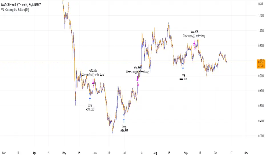
This strategy is back tested from 1 April 2022 to simulate how the strategy would work in a bear market and provides good returns.
Pairs that produce very strong results include ETH on the 5m timeframe, BNB on 5m timeframe, XRP on the 45m timeframe, MATIC on the 30m timeframe and MATIC on the 2H timeframe.
The strategy assumes each order is using 30% of the available coins to make the results more realistic and to simulate you only ran this strategy on 30% of your holdings. A trading fee of 0.1% is also taken into account and is aligned to the base fee applied on Binance.
Cari dalam skrip untuk "Exponential"
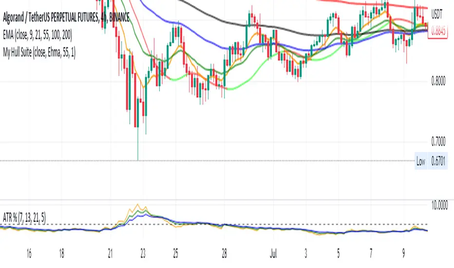
EMA curvesPlot EMAs for lengths 9, 21, 55 ,100, 200
An exponential moving average (EMA) is a type of moving average (MA) that places a greater weight and significance on the most recent data points. The exponential moving average is also referred to as the exponentially weighted moving average. An exponentially weighted moving average reacts more significantly to recent price changes than a simple moving average simple moving average (SMA), which applies an equal weight to all observations in the period.
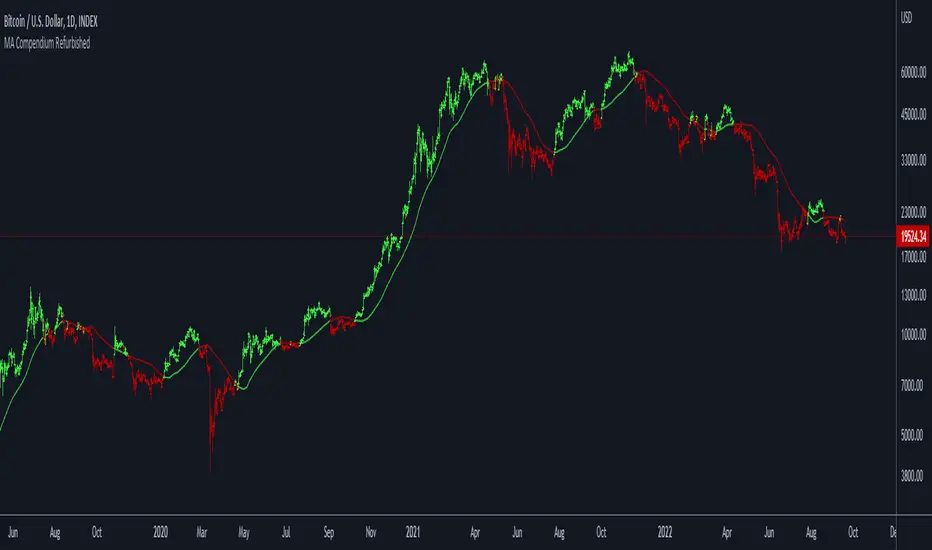
Moving Average Compendium RefurbishedThis is my effort to bring together in a single script the widest range of moving averages possible.
I aggregated the calculation of averages within a library.
For more information about the library follow the link:
Basically this indicator is the visual result of this library.
You can choose the moving average and the script updates the chart as per the type.
The unique parameters of certain moving averages remain at their default values.
To have a rainbow of moving averages I also made an indicator:
Available moving averages:
AARMA = 'Adaptive Autonomous Recursive Moving Average'
ADEMA = '* Alpha-Decreasing Exponential Moving Average'
AHMA = 'Ahrens Moving Average'
ALMA = 'Arnaud Legoux Moving Average'
ALSMA = 'Adaptive Least Squares'
AUTOL = 'Auto-Line'
CMA = 'Corrective Moving average'
CORMA = 'Correlation Moving Average Price'
COVWEMA = 'Coefficient of Variation Weighted Exponential Moving Average'
COVWMA = 'Coefficient of Variation Weighted Moving Average'
DEMA = 'Double Exponential Moving Average'
DONCHIAN = 'Donchian Middle Channel'
EDMA = 'Exponentially Deviating Moving Average'
EDSMA = 'Ehlers Dynamic Smoothed Moving Average'
EFRAMA = '* Ehlrs Modified Fractal Adaptive Moving Average'
EHMA = 'Exponential Hull Moving Average'
EMA = 'Exponential Moving Average'
EPMA = 'End Point Moving Average'
ETMA = 'Exponential Triangular Moving Average'
EVWMA = 'Elastic Volume Weighted Moving Average'
FAMA = 'Following Adaptive Moving Average'
FIBOWMA = 'Fibonacci Weighted Moving Average'
FISHLSMA = 'Fisher Least Squares Moving Average'
FRAMA = 'Fractal Adaptive Moving Average'
GMA = 'Geometric Moving Average'
HKAMA = 'Hilbert based Kaufman\'s Adaptive Moving Average'
HMA = 'Hull Moving Average'
JURIK = 'Jurik Moving Average'
KAMA = 'Kaufman\'s Adaptive Moving Average'
LC_LSMA = '1LC-LSMA (1 line code lsma with 3 functions)'
LEOMA = 'Leo Moving Average'
LINWMA = 'Linear Weighted Moving Average'
LSMA = 'Least Squares Moving Average'
MAMA = 'MESA Adaptive Moving Average'
MCMA = 'McNicholl Moving Average'
MEDIAN = 'Median'
REGMA = 'Regularized Exponential Moving Average'
REMA = 'Range EMA'
REPMA = 'Repulsion Moving Average'
RMA = 'Relative Moving Average'
RSIMA = 'RSI Moving average'
RVWAP = '* Rolling VWAP'
SMA = 'Simple Moving Average'
SMMA = 'Smoothed Moving Average'
SRWMA = 'Square Root Weighted Moving Average'
SW_MA = 'Sine-Weighted Moving Average'
SWMA = '* Symmetrically Weighted Moving Average'
TEMA = 'Triple Exponential Moving Average'
THMA = 'Triple Hull Moving Average'
TREMA = 'Triangular Exponential Moving Average'
TRSMA = 'Triangular Simple Moving Average'
TT3 = 'Tillson T3'
VAMA = 'Volatility Adjusted Moving Average'
VIDYA = 'Variable Index Dynamic Average'
VWAP = '* VWAP'
VWMA = 'Volume-weighted Moving Average'
WMA = 'Weighted Moving Average'
WWMA = 'Welles Wilder Moving Average'
XEMA = 'Optimized Exponential Moving Average'
ZEMA = 'Zero-Lag Exponential Moving Average'
ZSMA = 'Zero-Lag Simple Moving Average'
Moving Averages RefurbishedIntroduction
This is a collection of multiple moving averages, where you can have a rainbow of moving averages with different types that can be defined by the user.
There are already other indicators in this rainbow style, however certain averages are absent in certain indicators and present in others,
needing the merge to have a more complete solution.
Resources
Here there is the possibility to individually define each moving average.
In addition, it is possible to adjust some details, such as themes, coloring and periods.
Regarding the calculation of averages, credit goes to the following authors.
What I've done here is to group these averages together and allow them to combine.
Credits
TradingView
PineCoders
CrackingCryptocurrency
MightyZinger
Alex Orekhov (everget)
alexgrover
paragjyoti2012
Moving averages available
1. Exponential Moving Average
2. Simple Moving Average
3. Relative Moving Average
4. Weighted Moving Average
5. Ehlers Dynamic Smoothed Moving Average
6. Double Exponential Moving Average
7. Triple Exponential Moving Average
8. Smoothed Moving Average
9. Hull Moving Average
10. Fractal Adaptive Moving Average
11. Kaufman's Adaptive Moving Average
12. Volatility Adjusted Moving Average
13. Jurik Moving Average
14. Optimized Exponential Moving Average
15. Exponential Hull Moving Average
16. Arnaud Legoux Moving Average
17. Coefficient of Variation Weighted Exponential Moving Average
18. Coefficient of Variation Weighted Moving Average
19. * Ehlrs Modified Fractal Adaptive Moving Average
20. Exponential Triangular Moving Average
21. Least Squares Moving Average
22. RSI Moving average
23. Simple Triangular Moving Average
24. Triple Hull Moving Average
25. Variable Index Dynamic Average
26. Volume-weighted Moving Average
27. Zero-Lag Exponential Moving Average
28. Zero-Lag Simple Moving Average
29. Elastic Volume Weighted Moving Average
30. Tillson T3
31. Geometric Moving Average
32. Welles Wilder Moving Average
33. Adjusted Moving Average
34. Corrective Moving average
35. Exponentially Deviating Moving Average
36. EMA Range
37. Sine-Weighted Moving Average
38. Adaptive Moving Average TABLE
39. Following Adaptive Moving Average
40. Hilbert based Kaufman's Adaptive Moving Average
41. Median
42. * VWAP
43. * Rolling VWAP
44. Triangular Simple Moving Average
45. Triangular Exponential Moving Average
46. Moving Average Price Correlation
47. Regularized Exponential Moving Average
48. Repulsion Moving Average
49. * Symmetrically Weighted Moving Average
* fixed period averages

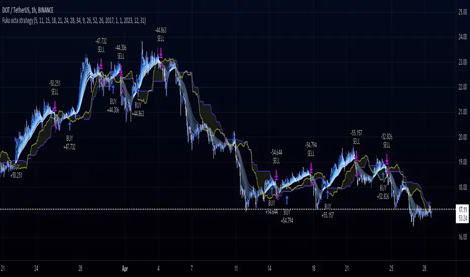
Fukuiz Octa-EMA + Ichimoku (Strategy)This strategy is based EMA of 8 different period and Ichimoku Cloud which works better in 1hr 4hr and daily time frame.
#A brief introduction to Ichimoku #
The Ichimoku Cloud is a collection of technical indicators that show support and resistance levels, as well as momentum and trend direction. It does this by taking multiple averages and plotting them on a chart. It also uses these figures to compute a “cloud” that attempts to forecast where the price may find support or resistance in the future.
#A brief introduction to EMA#
An exponential moving average ( EMA ) is a type of moving average (MA) that places a greater weight and significance on the most recent data points. The exponential moving average is also referred to as the exponentially weighted moving average . An exponentially weighted moving average reacts more significantly to recent price changes than a simple moving average ( SMA ), which applies an equal weight to all observations in the period.
#How to use#
The strategy will give entry points itself, you can monitor and take profit manually(recommended), or you can use the exit setup.
EMA (Color) = Bullish trend
EMA (Gray) = Bearish trend
#Condition#
Buy = All Ema (color) above the cloud.
SELL= All Ema turn to gray color.
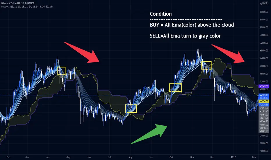
Fukuiz Octa-EMA + IchimokuThis indicator base on EMA of 8 different period and Ichimoku Cloud.
#A brief introduction to Ichimoku #
The Ichimoku Cloud is a collection of technical indicators that show support and resistance levels, as well as momentum and trend direction. It does this by taking multiple averages and plotting them on a chart. It also uses these figures to compute a “cloud” that attempts to forecast where the price may find support or resistance in the future.
#A brief introduction to EMA#
An exponential moving average (EMA) is a type of moving average (MA) that places a greater weight and significance on the most recent data points. The exponential moving average is also referred to as the exponentially weighted moving average. An exponentially weighted moving average reacts more significantly to recent price changes than a simple moving average (SMA), which applies an equal weight to all observations in the period.
I combine this together to help you reduce the false signals in Ichimoku.
#How to use#
EMA (Color) = Bullish trend
EMA (Gray) = Bearish trend
#Buy condition#
Buy = All Ema(color) above the cloud.
#Sell condition#
SELL= All Ema turn to gray color.
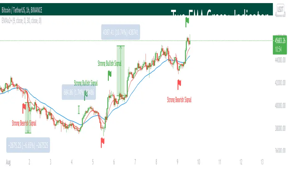
Two EMA Cross+ IndicatorHello traders!
Today we gonna demonstrate out heuristic of classical EMA Indicator. We decided to simplify your trading staff and add some meta data. So, let’s look at it from the very beginning and initially speak about what EMA is and then I’ll tell you why our indicator is extremely convenient and useful.
So, what is EMA? An exponential moving average ( EMA ) is a type of moving average (MA) that places a greater weight and significance on the most recent data points. The exponential moving average is also referred to as the exponentially weighted moving average . An exponentially weighted moving average reacts more significantly to recent price changes than a simple moving average ( SMA ), which applies an equal weight to all observations in the period.
Key takeaways:
-The EMA is a moving average that places a greater weight and significance on the most recent data points.
-Like all moving averages, this technical indicator is used to produce buy and sell signals based on crossovers and divergences from the historical average.
As you know, EMA Cross is one of basic and most popular Entry Indicators. It’s kinda easy to understand and even easier to use. This indicator consists of two EMAs - fast (red line) and slow (blue line). Fast EMA is EMA of less length that the fast EMA (default parameter is 9). Thus, it reacts the price change more actively than the slow. We can say that it takes into consideration the most actual price movements. Speaking about slow EMA (default parameter is 30) it’s more inert and it’s more difficult to change its action vastly. We can say that the EMA «looks» at the historical data more accurate, but doesn’t forget about actual price movements.
But how it works? Trivial. When the fast EMA crosses the slow bellow, it provides bearish signal, whereas when it crosses it above, it’s bullish signal. Even more, we added some «confirmation» factor. As you know, when the price is above the slow EMA, the slow EMA plays the role of support line for price and means that the price is in uptrend. Thus, when we see the cross above and it takes place under the price, we called it «strong Bullish Signal». When the price is bellow the slow EMA, slow EMA is resistance. Thus, when we see the cross bellow and it’s under the slow EMA, we called it «strong Bearish Signal».
To make your trading process easier, we plotted the places of crosses on the chart and added the descriptions of the crosses. The flags mean the place of cross. The default parameters have nice backtest on 1H chart. However, you can also change them depending on your goals and the time period. The places of cross looks like flags (red flag is «bearish» cross, green - «bullish»). As you can see, it’s really convenient.
I hope you’ll enjoy our heuristic of classical EMA Cross. We are sure that the meta data that we are taking into consideration makes the signals more accurate and the deals more profitable. The SkyRock Team with support of Trading View try to make your trading process more successful and profitable. Every day we works in conjunction to boost both your skills and trading balance. We hope, it’s really useful for you, dear traders!
MyLibraryLibrary "MyLibrary"
This library contains various trading strategies and utility functions for Pine Script.
simple_moving_average(src, length)
simple_moving_average
@description Calculates the Simple Moving Average (SMA) of a given series.
Parameters:
src (float) : (series float) The input series (e.g., close prices).
length (int) : (int) The number of periods to use for the SMA calculation.
Returns: (series float) The calculated SMA series.
exponential_moving_average(src, length)
exponential_moving_average
@description Calculates the Exponential Moving Average (EMA) of a given series.
Parameters:
src (float) : (series float) The input series (e.g., close prices).
length (simple int) : (int) The number of periods to use for the EMA calculation.
Returns: (series float) The calculated EMA series.
safe_division(numerator, denominator)
safe_division
@description Performs division with error handling for division by zero.
Parameters:
numerator (float) : (float) The numerator for the division.
denominator (float) : (float) The denominator for the division.
Returns: (float) The result of the division, or na if the denominator is zero.
strategy_moving_average_crossover(shortLength, longLength)
strategy_moving_average_crossover
@description Implements a Moving Average Crossover strategy.
Parameters:
shortLength (int) : (int) The length for the short period SMA.
longLength (int) : (int) The length for the long period SMA.
Returns: (series float, series float, series bool, series bool) The short SMA, long SMA, crossover signals, and crossunder signals.
strategy_rsi(rsiLength, overbought, oversold)
strategy_rsi
@description Implements an RSI-based trading strategy.
Parameters:
rsiLength (simple int) : (int) The length for the RSI calculation.
overbought (float) : (float) The overbought threshold.
oversold (float) : (float) The oversold threshold.
Returns: (series float, series bool, series bool) The RSI values, long signals, and short signals.
ichimoku_cloud(convPeriod, basePeriod, spanBPeriod, laggingSpanPeriod)
ichimoku_cloud
@description Computes Ichimoku Cloud components.
Parameters:
convPeriod (int) : (int) The conversion line period.
basePeriod (int) : (int) The base line period.
spanBPeriod (int)
laggingSpanPeriod (int)
Returns: (series float, series float, series float, series float, series float) The conversion line, base line, leading span A, leading span B, and lagging span.
strategy_ichimoku_conversion_baseline()
strategy_ichimoku_conversion_baseline
@description Implements an Ichimoku Conversion Line and Baseline strategy.
Returns: (series float, series float, series bool, series bool) The conversion line, baseline, crossover signals, and crossunder signals.
debug_print(labelText, value, barIndex)
debug_print
@description Prints values to the chart for debugging purposes.
Parameters:
labelText (string) : (string) The label text.
value (float) : (float) The value to display.
barIndex (int) : (int) The bar index where the label should be displayed.

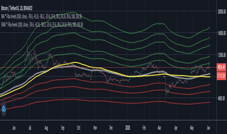
BAERMThe Bitcoin Auto-correlation Exchange Rate Model: A Novel Two Step Approach
THIS IS NOT FINANCIAL ADVICE. THIS ARTICLE IS FOR EDUCATIONAL AND ENTERTAINMENT PURPOSES ONLY.
If you enjoy this software and information, please consider contributing to my lightning address
Prelude
It has been previously established that the Bitcoin daily USD exchange rate series is extremely auto-correlated
In this article, we will utilise this fact to build a model for Bitcoin/USD exchange rate. But not a model for predicting the exchange rate, but rather a model to understand the fundamental reasons for the Bitcoin to have this exchange rate to begin with.
This is a model of sound money, scarcity and subjective value.
Introduction
Bitcoin, a decentralised peer to peer digital value exchange network, has experienced significant exchange rate fluctuations since its inception in 2009. In this article, we explore a two-step model that reasonably accurately captures both the fundamental drivers of Bitcoin’s value and the cyclical patterns of bull and bear markets. This model, whilst it can produce forecasts, is meant more of a way of understanding past exchange rate changes and understanding the fundamental values driving the ever increasing exchange rate. The forecasts from the model are to be considered inconclusive and speculative only.
Data preparation
To develop the BAERM, we used historical Bitcoin data from Coin Metrics, a leading provider of Bitcoin market data. The dataset includes daily USD exchange rates, block counts, and other relevant information. We pre-processed the data by performing the following steps:
Fixing date formats and setting the dataset’s time index
Generating cumulative sums for blocks and halving periods
Calculating daily rewards and total supply
Computing the log-transformed price
Step 1: Building the Base Model
To build the base model, we analysed data from the first two epochs (time periods between Bitcoin mining reward halvings) and regressed the logarithm of Bitcoin’s exchange rate on the mining reward and epoch. This base model captures the fundamental relationship between Bitcoin’s exchange rate, mining reward, and halving epoch.
where Yt represents the exchange rate at day t, Epochk is the kth epoch (for that t), and epsilont is the error term. The coefficients beta0, beta1, and beta2 are estimated using ordinary least squares regression.
Base Model Regression
We use ordinary least squares regression to estimate the coefficients for the betas in figure 2. In order to reduce the possibility of over-fitting and ensure there is sufficient out of sample for testing accuracy, the base model is only trained on the first two epochs. You will notice in the code we calculate the beta2 variable prior and call it “phaseplus”.
The code below shows the regression for the base model coefficients:
\# Run the regression
mask = df\ < 2 # we only want to use Epoch's 0 and 1 to estimate the coefficients for the base model
reg\_X = df.loc\ [mask, \ \].shift(1).iloc\
reg\_y = df.loc\ .iloc\
reg\_X = sm.add\_constant(reg\_X)
ols = sm.OLS(reg\_y, reg\_X).fit()
coefs = ols.params.values
print(coefs)
The result of this regression gives us the coefficients for the betas of the base model:
\
or in more human readable form: 0.029, 0.996869586, -0.00043. NB that for the auto-correlation/momentum beta, we did NOT round the significant figures at all. Since the momentum is so important in this model, we must use all available significant figures.
Fundamental Insights from the Base Model
Momentum effect: The term 0.997 Y suggests that the exchange rate of Bitcoin on a given day (Yi) is heavily influenced by the exchange rate on the previous day. This indicates a momentum effect, where the price of Bitcoin tends to follow its recent trend.
Momentum effect is a phenomenon observed in various financial markets, including stocks and other commodities. It implies that an asset’s price is more likely to continue moving in its current direction, either upwards or downwards, over the short term.
The momentum effect can be driven by several factors:
Behavioural biases: Investors may exhibit herding behaviour or be subject to cognitive biases such as confirmation bias, which could lead them to buy or sell assets based on recent trends, reinforcing the momentum.
Positive feedback loops: As more investors notice a trend and act on it, the trend may gain even more traction, leading to a self-reinforcing positive feedback loop. This can cause prices to continue moving in the same direction, further amplifying the momentum effect.
Technical analysis: Many traders use technical analysis to make investment decisions, which often involves studying historical exchange rate trends and chart patterns to predict future exchange rate movements. When a large number of traders follow similar strategies, their collective actions can create and reinforce exchange rate momentum.
Impact of halving events: In the Bitcoin network, new bitcoins are created as a reward to miners for validating transactions and adding new blocks to the blockchain. This reward is called the block reward, and it is halved approximately every four years, or every 210,000 blocks. This event is known as a halving.
The primary purpose of halving events is to control the supply of new bitcoins entering the market, ultimately leading to a capped supply of 21 million bitcoins. As the block reward decreases, the rate at which new bitcoins are created slows down, and this can have significant implications for the price of Bitcoin.
The term -0.0004*(50/(2^epochk) — (epochk+1)²) accounts for the impact of the halving events on the Bitcoin exchange rate. The model seems to suggest that the exchange rate of Bitcoin is influenced by a function of the number of halving events that have occurred.
Exponential decay and the decreasing impact of the halvings: The first part of this term, 50/(2^epochk), indicates that the impact of each subsequent halving event decays exponentially, implying that the influence of halving events on the Bitcoin exchange rate diminishes over time. This might be due to the decreasing marginal effect of each halving event on the overall Bitcoin supply as the block reward gets smaller and smaller.
This is antithetical to the wrong and popular stock to flow model, which suggests the opposite. Given the accuracy of the BAERM, this is yet another reason to question the S2F model, from a fundamental perspective.
The second part of the term, (epochk+1)², introduces a non-linear relationship between the halving events and the exchange rate. This non-linear aspect could reflect that the impact of halving events is not constant over time and may be influenced by various factors such as market dynamics, speculation, and changing market conditions.
The combination of these two terms is expressed by the graph of the model line (see figure 3), where it can be seen the step from each halving is decaying, and the step up from each halving event is given by a parabolic curve.
NB - The base model has been trained on the first two halving epochs and then seeded (i.e. the first lag point) with the oldest data available.
Constant term: The constant term 0.03 in the equation represents an inherent baseline level of growth in the Bitcoin exchange rate.
In any linear or linear-like model, the constant term, also known as the intercept or bias, represents the value of the dependent variable (in this case, the log-scaled Bitcoin USD exchange rate) when all the independent variables are set to zero.
The constant term indicates that even without considering the effects of the previous day’s exchange rate or halving events, there is a baseline growth in the exchange rate of Bitcoin. This baseline growth could be due to factors such as the network’s overall growth or increasing adoption, or changes in the market structure (more exchanges, changes to the regulatory environment, improved liquidity, more fiat on-ramps etc).
Base Model Regression Diagnostics
Below is a summary of the model generated by the OLS function
OLS Regression Results
\==============================================================================
Dep. Variable: logprice R-squared: 0.999
Model: OLS Adj. R-squared: 0.999
Method: Least Squares F-statistic: 2.041e+06
Date: Fri, 28 Apr 2023 Prob (F-statistic): 0.00
Time: 11:06:58 Log-Likelihood: 3001.6
No. Observations: 2182 AIC: -5997.
Df Residuals: 2179 BIC: -5980.
Df Model: 2
Covariance Type: nonrobust
\==============================================================================
coef std err t P>|t| \
\------------------------------------------------------------------------------
const 0.0292 0.009 3.081 0.002 0.011 0.048
logprice 0.9969 0.001 1012.724 0.000 0.995 0.999
phaseplus -0.0004 0.000 -2.239 0.025 -0.001 -5.3e-05
\==============================================================================
Omnibus: 674.771 Durbin-Watson: 1.901
Prob(Omnibus): 0.000 Jarque-Bera (JB): 24937.353
Skew: -0.765 Prob(JB): 0.00
Kurtosis: 19.491 Cond. No. 255.
\==============================================================================
Below we see some regression diagnostics along with the regression itself.
Diagnostics: We can see that the residuals are looking a little skewed and there is some heteroskedasticity within the residuals. The coefficient of determination, or r2 is very high, but that is to be expected given the momentum term. A better r2 is manually calculated by the sum square of the difference of the model to the untrained data. This can be achieved by the following code:
\# Calculate the out-of-sample R-squared
oos\_mask = df\ >= 2
oos\_actual = df.loc\
oos\_predicted = df.loc\
residuals\_oos = oos\_actual - oos\_predicted
SSR = np.sum(residuals\_oos \*\* 2)
SST = np.sum((oos\_actual - oos\_actual.mean()) \*\* 2)
R2\_oos = 1 - SSR/SST
print("Out-of-sample R-squared:", R2\_oos)
The result is: 0.84, which indicates a very close fit to the out of sample data for the base model, which goes some way to proving our fundamental assumption around subjective value and sound money to be accurate.
Step 2: Adding the Damping Function
Next, we incorporated a damping function to capture the cyclical nature of bull and bear markets. The optimal parameters for the damping function were determined by regressing on the residuals from the base model. The damping function enhances the model’s ability to identify and predict bull and bear cycles in the Bitcoin market. The addition of the damping function to the base model is expressed as the full model equation.
This brings me to the question — why? Why add the damping function to the base model, which is arguably already performing extremely well out of sample and providing valuable insights into the exchange rate movements of Bitcoin.
Fundamental reasoning behind the addition of a damping function:
Subjective Theory of Value: The cyclical component of the damping function, represented by the cosine function, can be thought of as capturing the periodic fluctuations in market sentiment. These fluctuations may arise from various factors, such as changes in investor risk appetite, macroeconomic conditions, or technological advancements. Mathematically, the cyclical component represents the frequency of these fluctuations, while the phase shift (α and β) allows for adjustments in the alignment of these cycles with historical data. This flexibility enables the damping function to account for the heterogeneity in market participants’ preferences and expectations, which is a key aspect of the subjective theory of value.
Time Preference and Market Cycles: The exponential decay component of the damping function, represented by the term e^(-0.0004t), can be linked to the concept of time preference and its impact on market dynamics. In financial markets, the discounting of future cash flows is a common practice, reflecting the time value of money and the inherent uncertainty of future events. The exponential decay in the damping function serves a similar purpose, diminishing the influence of past market cycles as time progresses. This decay term introduces a time-dependent weight to the cyclical component, capturing the dynamic nature of the Bitcoin market and the changing relevance of past events.
Interactions between Cyclical and Exponential Decay Components: The interplay between the cyclical and exponential decay components in the damping function captures the complex dynamics of the Bitcoin market. The damping function effectively models the attenuation of past cycles while also accounting for their periodic nature. This allows the model to adapt to changing market conditions and to provide accurate predictions even in the face of significant volatility or structural shifts.
Now we have the fundamental reasoning for the addition of the function, we can explore the actual implementation and look to other analogies for guidance —
Financial and physical analogies to the damping function:
Mathematical Aspects: The exponential decay component, e^(-0.0004t), attenuates the amplitude of the cyclical component over time. This attenuation factor is crucial in modelling the diminishing influence of past market cycles. The cyclical component, represented by the cosine function, accounts for the periodic nature of market cycles, with α determining the frequency of these cycles and β representing the phase shift. The constant term (+3) ensures that the function remains positive, which is important for practical applications, as the damping function is added to the rest of the model to obtain the final predictions.
Analogies to Existing Damping Functions: The damping function in the BAERM is similar to damped harmonic oscillators found in physics. In a damped harmonic oscillator, an object in motion experiences a restoring force proportional to its displacement from equilibrium and a damping force proportional to its velocity. The equation of motion for a damped harmonic oscillator is:
x’’(t) + 2γx’(t) + ω₀²x(t) = 0
where x(t) is the displacement, ω₀ is the natural frequency, and γ is the damping coefficient. The damping function in the BAERM shares similarities with the solution to this equation, which is typically a product of an exponential decay term and a sinusoidal term. The exponential decay term in the BAERM captures the attenuation of past market cycles, while the cosine term represents the periodic nature of these cycles.
Comparisons with Financial Models: In finance, damped oscillatory models have been applied to model interest rates, stock prices, and exchange rates. The famous Black-Scholes option pricing model, for instance, assumes that stock prices follow a geometric Brownian motion, which can exhibit oscillatory behavior under certain conditions. In fixed income markets, the Cox-Ingersoll-Ross (CIR) model for interest rates also incorporates mean reversion and stochastic volatility, leading to damped oscillatory dynamics.
By drawing on these analogies, we can better understand the technical aspects of the damping function in the BAERM and appreciate its effectiveness in modelling the complex dynamics of the Bitcoin market. The damping function captures both the periodic nature of market cycles and the attenuation of past events’ influence.
Conclusion
In this article, we explored the Bitcoin Auto-correlation Exchange Rate Model (BAERM), a novel 2-step linear regression model for understanding the Bitcoin USD exchange rate. We discussed the model’s components, their interpretations, and the fundamental insights they provide about Bitcoin exchange rate dynamics.
The BAERM’s ability to capture the fundamental properties of Bitcoin is particularly interesting. The framework underlying the model emphasises the importance of individuals’ subjective valuations and preferences in determining prices. The momentum term, which accounts for auto-correlation, is a testament to this idea, as it shows that historical price trends influence market participants’ expectations and valuations. This observation is consistent with the notion that the price of Bitcoin is determined by individuals’ preferences based on past information.
Furthermore, the BAERM incorporates the impact of Bitcoin’s supply dynamics on its price through the halving epoch terms. By acknowledging the significance of supply-side factors, the model reflects the principles of sound money. A limited supply of money, such as that of Bitcoin, maintains its value and purchasing power over time. The halving events, which reduce the block reward, play a crucial role in making Bitcoin increasingly scarce, thus reinforcing its attractiveness as a store of value and a medium of exchange.
The constant term in the model serves as the baseline for the model’s predictions and can be interpreted as an inherent value attributed to Bitcoin. This value emphasizes the significance of the underlying technology, network effects, and Bitcoin’s role as a medium of exchange, store of value, and unit of account. These aspects are all essential for a sound form of money, and the model’s ability to account for them further showcases its strength in capturing the fundamental properties of Bitcoin.
The BAERM offers a potential robust and well-founded methodology for understanding the Bitcoin USD exchange rate, taking into account the key factors that drive it from both supply and demand perspectives.
In conclusion, the Bitcoin Auto-correlation Exchange Rate Model provides a comprehensive fundamentally grounded and hopefully useful framework for understanding the Bitcoin USD exchange rate.

Debye-Einstein Trend Oscillator [Dual Mode] | IkkeOmarDebye-Einstein Trend Oscillator
Indicator Settings Guide
Visual Settings View Mode: Switches the chart display. Select "Standard Flow" to see the raw physics energy bars and crossover lines. Select "Trend Diff (MACD)" to see the histogram that highlights momentum shifts and chaos spikes.
Physics Engine Trend Lookback: Defines the "Mass" of the trend. This sets the long-term baseline (default 1500 bars). Higher values filter out noise and focus only on macro-cycles; lower values make the system faster but noisier. Chaos Threshold (%): Controls the trigger for the Einstein (Chaos) state. Set to 95, only the top 5% of highest-energy volume events will trigger the vertical white spikes. Lowering this value makes the system more sensitive to volatility.
Flow Moving Averages MA Type: Choose between SMA (Simple) or EMA (Exponential) for the smoothing calculation. Fast / Slow Length: These settings determine the sensitivity of the momentum logic. The difference between these two lengths creates the histogram in "Trend Diff" mode.
1. Concept & Theoretical Basis
This script applies principles from Solid State Physics—specifically the Debye and Einstein models of specific heat capacity—to financial market trend analysis.
The core hypothesis is that market trends behave like physical lattices:
Low Energy State (Debye Model): The market moves in a coordinated, wave-like manner (phonons). Trends are sustainable and correlated.
High Energy State (Einstein Model): The market becomes chaotic. Individual participants (atoms) vibrate independently and violently. This represents capitulation or euphoria.
We model "Price" as the position of particles and "Volume × Range" as the thermal energy (Temperature) entering the system.
2. Implementation Models
We constructed the oscillator using three primary physical components:
A. The Trend Vector (Mass)
We assume the "Mass" of the market is its inertia relative to a long-term baseline.
Model: Distance from a 1500-period SMA, normalized by ATR.
Assumption: Price deviation from a deep baseline indicates the magnitude of the trend "force."
B. Thermodynamics (Temperature)
We define "Work" as Volume * True Range.
Temperature (T): The Percentile Rank of this Work over the lookback period (1500 bars).
Assumption: High volume combined with high range equals high thermal energy.
C. The Dual Regimes (Amplifiers)
This is the engine of the script. We apply a scalar multiplier to the Trend Vector based on the current Temperature (T).
Debye Regime (Sustainable): When T is below the critical threshold (95%), we use a polynomial function (T^2). This mimics the Debye T^3 law where energy scales smoothly.
Effect: Smoothly amplifies standard trends.
Einstein Regime (Chaos): When T breaches the critical threshold (95%), we switch to an exponential function derived from the Einstein Solid model.
Effect: Creates massive vertical spikes during trend exhaustions or breakouts.
3. Code Explanation
The Physics Scalars
debye_amp(t) => 1.0 + (math.pow(t, 2) * 5.0)
Defines the sustainable state multiplier. Squaring the temperature t creates a non-linear but smooth response curve that gradually increases with volatility.
einstein_amp(t) => 1.0 + ((1.0 / (math.exp(1.0 / t_safe) - 1.0)) * 15.0)
Deep Dive: This function applies the Bose-Einstein distribution formula (1 / (e^(1/T) - 1)).
The Physics: In quantum mechanics, this formula calculates the occupancy of energy states. At low temperatures, the value is effectively zero (the "frozen" state).
The Function: As our market "Temperature" (T) rises, the denominator shrinks, causing the output to grow exponentially.
The Result: This mathematically forces the system to ignore low-volatility noise but react explosively once the "Boiling Point" is reached, creating the vertical spikes seen on the chart.
is_einstein = (T * 100) >= thresh_einstein
A boolean check that determines if the current market energy (Temperature) has exceeded the user-defined chaos threshold (default 95%).
physics_scalar = is_einstein ? einstein_amp(T) : debye_amp(T)
The regime switch. If the threshold is breached, the system applies the exponential Einstein scalar; otherwise, it applies the polynomial Debye scalar.
Trend Differentiation Logic
final_flow = trend_vector * physics_scalar
Calculates the primary oscillator value by multiplying the directional Trend Vector (Mass) by the active Physics Scalar (Energy).
diff_val = ma_fast - ma_slow
Calculates the momentum of the flow itself by subtracting the Slow Moving Average from the Fast Moving Average. This creates the MACD-style histogram.
4. Visual Reporting & Chart Analysis
Referring to the generated charts (Trend Diff Mode):
The Histogram: Represents the diff_val (Fast MA - Slow MA).
Cyan/Pink: Standard trend momentum (Debye mode).
White Spikes: These represent the Einstein Threshold (Chaos). These spikes generally appear at local bottoms or explosive breakout points, confirming that "Temperature" has exceeded the 95th percentile.
Zero Line: Crossing the zero line implies the trend momentum has shifted (Fast MA crossed Slow MA).
5. Assumptions & Limitations
A. The "Always in Trend" Bias
The "Trend Diff" mode calculates the delta between two moving averages of the flow.
Risk: MAs are laggy by definition. By using a 200/500 MA combo on the oscillator, we are smoothing the data significantly.
Consequence: In a ranging market, the MAs will converge near zero. However, if a sudden burst of Volume enters (Temperature rises) without price moving much, the Einstein scalar will trigger. This may amplify a small move into a large signal, implying a trend where there is only volatility.
B. Lag
The lookback period is 1500 bars. This is a "Macro" trend system. It will not react quickly to short-term reversals unless the Volume/Range shock is massive enough to trigger the Einstein scalar immediately.
Example "physics values"
In the Standard Flow view, the vertical columns represent the raw energy of the trend—Teal and Red bars indicate normal, sustainable market movement (Debye state), while bright Lime and Fuchsia bars signal chaotic, high-volatility events (Einstein state). The height of these bars shows the combined strength of price direction and volume. Overlaying these columns are two moving averages, a fast Blue line and a slow Red line, which smooth out this data to show the underlying momentum. When the Blue line crosses the Red line, it signals a shift in the trend's direction, while the color of the bars warns you if that move is stable or nearing exhaustion.

Chande Kroll Trend Strategy (SPX, 1H) | PINEINDICATORSThe "Chande Kroll Stop Strategy" is designed to optimize trading on the SPX using a 1-hour timeframe. This strategy effectively combines the Chande Kroll Stop indicator with a Simple Moving Average (SMA) to create a robust method for identifying long entry and exit points. This detailed description will explain the components, rationale, and usage to ensure compliance with TradingView's guidelines and help traders understand the strategy's utility and application.
Objective
The primary goal of this strategy is to identify potential long trading opportunities in the SPX by leveraging volatility-adjusted stop levels and trend-following principles. It aims to capture upward price movements while managing risk through dynamically calculated stops.
Chande Kroll Stop Parameters:
Calculation Mode: Offers "Linear" and "Exponential" options for position size calculation. The default mode is "Exponential."
Risk Multiplier: An adjustable multiplier for risk management and position sizing, defaulting to 5.
ATR Period: Defines the period for calculating the Average True Range (ATR), with a default of 10.
ATR Multiplier: A multiplier applied to the ATR to set stop levels, defaulting to 3.
Stop Length: Period used to determine the highest high and lowest low for stop calculation, defaulting to 21.
SMA Length: Period for the Simple Moving Average, defaulting to 21.
Calculation Details:
ATR Calculation: ATR is calculated over the specified period to measure market volatility.
Chande Kroll Stop Calculation:
High Stop: The highest high over the stop length minus the ATR multiplied by the ATR multiplier.
Low Stop: The lowest low over the stop length plus the ATR multiplied by the ATR multiplier.
SMA Calculation: The 21-period SMA of the closing price is used as a trend filter.
Entry and Exit Conditions:
Long Entry: A long position is initiated when the closing price crosses over the low stop and is above the 21-period SMA. This condition ensures that the market is trending upward and that the entry is made in the direction of the prevailing trend.
Exit Long: The long position is exited when the closing price falls below the high stop, indicating potential downward movement and protecting against significant drawdowns.
Position Sizing:
The quantity of shares to trade is calculated based on the selected calculation mode (linear or exponential) and the risk multiplier. This ensures position size is adjusted dynamically based on current market conditions and user-defined risk tolerance.
Exponential Mode: Quantity is calculated using the formula: riskMultiplier / lowestClose * 1000 * strategy.equity / strategy.initial_capital.
Linear Mode: Quantity is calculated using the formula: riskMultiplier / lowestClose * 1000.
Execution:
When the long entry condition is met, the strategy triggers a buy signal, and a long position is entered with the calculated quantity. An alert is generated to notify the trader.
When the exit condition is met, the strategy closes the position and triggers a sell signal, accompanied by an alert.
Plotting:
Buy Signals: Indicated with an upward triangle below the bar.
Sell Signals: Indicated with a downward triangle above the bar.
Application
This strategy is particularly effective for trading the SPX on a 1-hour timeframe, capitalizing on price movements by adjusting stop levels dynamically based on market volatility and trend direction.
Default Setup
Initial Capital: $1,000
Risk Multiplier: 5
ATR Period: 10
ATR Multiplier: 3
Stop Length: 21
SMA Length: 21
Commission: 0.01
Slippage: 3 Ticks
Backtesting Results
Backtesting indicates that the "Chande Kroll Stop Strategy" performs optimally on the SPX when applied to the 1-hour timeframe. The strategy's dynamic adjustment of stop levels helps manage risk effectively while capturing significant upward price movements. Backtesting was conducted with a realistic initial capital of $1,000, and commissions and slippage were included to ensure the results are not misleading.
Risk Management
The strategy incorporates risk management through dynamically calculated stop levels based on the ATR and a user-defined risk multiplier. This approach ensures that position sizes are adjusted according to market volatility, helping to mitigate potential losses. Trades are sized to risk a sustainable amount of equity, adhering to the guideline of risking no more than 5-10% per trade.
Usage Notes
Customization: Users can adjust the ATR period, ATR multiplier, stop length, and SMA length to better suit their trading style and risk tolerance.
Alerts: The strategy includes alerts for buy and sell signals to keep traders informed of potential entry and exit points.
Pyramiding: Although possible, the strategy yields the best results without pyramiding.
Justification of Components
The Chande Kroll Stop indicator and the 21-period SMA are combined to provide a robust framework for identifying long trading opportunities in trending markets. Here is why they work well together:
Chande Kroll Stop Indicator: This indicator provides dynamic stop levels that adapt to market volatility, allowing traders to set logical stop-loss levels that account for current price movements. It is particularly useful in volatile markets where fixed stops can be easily hit by random price fluctuations. By using the ATR, the stop levels adjust based on recent market activity, ensuring they remain relevant in varying market conditions.
21-Period SMA: The 21-period SMA acts as a trend filter to ensure trades are taken in the direction of the prevailing market trend. By requiring the closing price to be above the SMA for long entries, the strategy aligns itself with the broader market trend, reducing the risk of entering trades against the overall market direction. This helps to avoid false signals and ensures that the trades are in line with the dominant market movement.
Combining these two components creates a balanced approach that captures trending price movements while protecting against significant drawdowns through adaptive stop levels. The Chande Kroll Stop ensures that the stops are placed at levels that reflect current volatility, while the SMA filter ensures that trades are only taken when the market is trending in the desired direction.
Concepts Underlying Calculations
ATR (Average True Range): Used to measure market volatility, which informs the stop levels.
SMA (Simple Moving Average): Used to filter trades, ensuring positions are taken in the direction of the trend.
Chande Kroll Stop: Combines high and low price levels with ATR to create dynamic stop levels that adapt to market conditions.
Risk Disclaimer
Trading involves substantial risk, and most day traders incur losses. The "Chande Kroll Stop Strategy" is provided for informational and educational purposes only. Past performance is not indicative of future results. Users are advised to adjust and personalize this trading strategy to better match their individual trading preferences and risk tolerance.

Softmax Normalized T3 Histogram [Loxx]Softmax Normalized T3 Histogram is a T3 moving average that is morphed into a normalized oscillator from -1 to 1.
What is the Softmax function?
The softmax function, also known as softargmax: or normalized exponential function, converts a vector of K real numbers into a probability distribution of K possible outcomes. It is a generalization of the logistic function to multiple dimensions, and used in multinomial logistic regression. The softmax function is often used as the last activation function of a neural network to normalize the output of a network to a probability distribution over predicted output classes, based on Luce's choice axiom.
What is the T3 moving average?
Better Moving Averages Tim Tillson
November 1, 1998
Tim Tillson is a software project manager at Hewlett-Packard, with degrees in Mathematics and Computer Science. He has privately traded options and equities for 15 years.
Introduction
"Digital filtering includes the process of smoothing, predicting, differentiating, integrating, separation of signals, and removal of noise from a signal. Thus many people who do such things are actually using digital filters without realizing that they are; being unacquainted with the theory, they neither understand what they have done nor the possibilities of what they might have done."
This quote from R. W. Hamming applies to the vast majority of indicators in technical analysis . Moving averages, be they simple, weighted, or exponential, are lowpass filters; low frequency components in the signal pass through with little attenuation, while high frequencies are severely reduced.
"Oscillator" type indicators (such as MACD , Momentum, Relative Strength Index ) are another type of digital filter called a differentiator.
Tushar Chande has observed that many popular oscillators are highly correlated, which is sensible because they are trying to measure the rate of change of the underlying time series, i.e., are trying to be the first and second derivatives we all learned about in Calculus.
We use moving averages (lowpass filters) in technical analysis to remove the random noise from a time series, to discern the underlying trend or to determine prices at which we will take action. A perfect moving average would have two attributes:
It would be smooth, not sensitive to random noise in the underlying time series. Another way of saying this is that its derivative would not spuriously alternate between positive and negative values.
It would not lag behind the time series it is computed from. Lag, of course, produces late buy or sell signals that kill profits.
The only way one can compute a perfect moving average is to have knowledge of the future, and if we had that, we would buy one lottery ticket a week rather than trade!
Having said this, we can still improve on the conventional simple, weighted, or exponential moving averages. Here's how:
Two Interesting Moving Averages
We will examine two benchmark moving averages based on Linear Regression analysis.
In both cases, a Linear Regression line of length n is fitted to price data.
I call the first moving average ILRS, which stands for Integral of Linear Regression Slope. One simply integrates the slope of a linear regression line as it is successively fitted in a moving window of length n across the data, with the constant of integration being a simple moving average of the first n points. Put another way, the derivative of ILRS is the linear regression slope. Note that ILRS is not the same as a SMA ( simple moving average ) of length n, which is actually the midpoint of the linear regression line as it moves across the data.
We can measure the lag of moving averages with respect to a linear trend by computing how they behave when the input is a line with unit slope. Both SMA (n) and ILRS(n) have lag of n/2, but ILRS is much smoother than SMA .
Our second benchmark moving average is well known, called EPMA or End Point Moving Average. It is the endpoint of the linear regression line of length n as it is fitted across the data. EPMA hugs the data more closely than a simple or exponential moving average of the same length. The price we pay for this is that it is much noisier (less smooth) than ILRS, and it also has the annoying property that it overshoots the data when linear trends are present.
However, EPMA has a lag of 0 with respect to linear input! This makes sense because a linear regression line will fit linear input perfectly, and the endpoint of the LR line will be on the input line.
These two moving averages frame the tradeoffs that we are facing. On one extreme we have ILRS, which is very smooth and has considerable phase lag. EPMA has 0 phase lag, but is too noisy and overshoots. We would like to construct a better moving average which is as smooth as ILRS, but runs closer to where EPMA lies, without the overshoot.
A easy way to attempt this is to split the difference, i.e. use (ILRS(n)+EPMA(n))/2. This will give us a moving average (call it IE /2) which runs in between the two, has phase lag of n/4 but still inherits considerable noise from EPMA. IE /2 is inspirational, however. Can we build something that is comparable, but smoother? Figure 1 shows ILRS, EPMA, and IE /2.
Filter Techniques
Any thoughtful student of filter theory (or resolute experimenter) will have noticed that you can improve the smoothness of a filter by running it through itself multiple times, at the cost of increasing phase lag.
There is a complementary technique (called twicing by J.W. Tukey) which can be used to improve phase lag. If L stands for the operation of running data through a low pass filter, then twicing can be described by:
L' = L(time series) + L(time series - L(time series))
That is, we add a moving average of the difference between the input and the moving average to the moving average. This is algebraically equivalent to:
2L-L(L)
This is the Double Exponential Moving Average or DEMA , popularized by Patrick Mulloy in TASAC (January/February 1994).
In our taxonomy, DEMA has some phase lag (although it exponentially approaches 0) and is somewhat noisy, comparable to IE /2 indicator.
We will use these two techniques to construct our better moving average, after we explore the first one a little more closely.
Fixing Overshoot
An n-day EMA has smoothing constant alpha=2/(n+1) and a lag of (n-1)/2.
Thus EMA (3) has lag 1, and EMA (11) has lag 5. Figure 2 shows that, if I am willing to incur 5 days of lag, I get a smoother moving average if I run EMA (3) through itself 5 times than if I just take EMA (11) once.
This suggests that if EPMA and DEMA have 0 or low lag, why not run fast versions (eg DEMA (3)) through themselves many times to achieve a smooth result? The problem is that multiple runs though these filters increase their tendency to overshoot the data, giving an unusable result. This is because the amplitude response of DEMA and EPMA is greater than 1 at certain frequencies, giving a gain of much greater than 1 at these frequencies when run though themselves multiple times. Figure 3 shows DEMA (7) and EPMA(7) run through themselves 3 times. DEMA^3 has serious overshoot, and EPMA^3 is terrible.
The solution to the overshoot problem is to recall what we are doing with twicing:
DEMA (n) = EMA (n) + EMA (time series - EMA (n))
The second term is adding, in effect, a smooth version of the derivative to the EMA to achieve DEMA . The derivative term determines how hot the moving average's response to linear trends will be. We need to simply turn down the volume to achieve our basic building block:
EMA (n) + EMA (time series - EMA (n))*.7;
This is algebraically the same as:
EMA (n)*1.7-EMA( EMA (n))*.7;
I have chosen .7 as my volume factor, but the general formula (which I call "Generalized Dema") is:
GD (n,v) = EMA (n)*(1+v)-EMA( EMA (n))*v,
Where v ranges between 0 and 1. When v=0, GD is just an EMA , and when v=1, GD is DEMA . In between, GD is a cooler DEMA . By using a value for v less than 1 (I like .7), we cure the multiple DEMA overshoot problem, at the cost of accepting some additional phase delay. Now we can run GD through itself multiple times to define a new, smoother moving average T3 that does not overshoot the data:
T3(n) = GD ( GD ( GD (n)))
In filter theory parlance, T3 is a six-pole non-linear Kalman filter. Kalman filters are ones which use the error (in this case (time series - EMA (n)) to correct themselves. In Technical Analysis , these are called Adaptive Moving Averages; they track the time series more aggressively when it is making large moves.
Included:
Bar coloring
Signals
Alerts
Loxx's Expanded Source Types
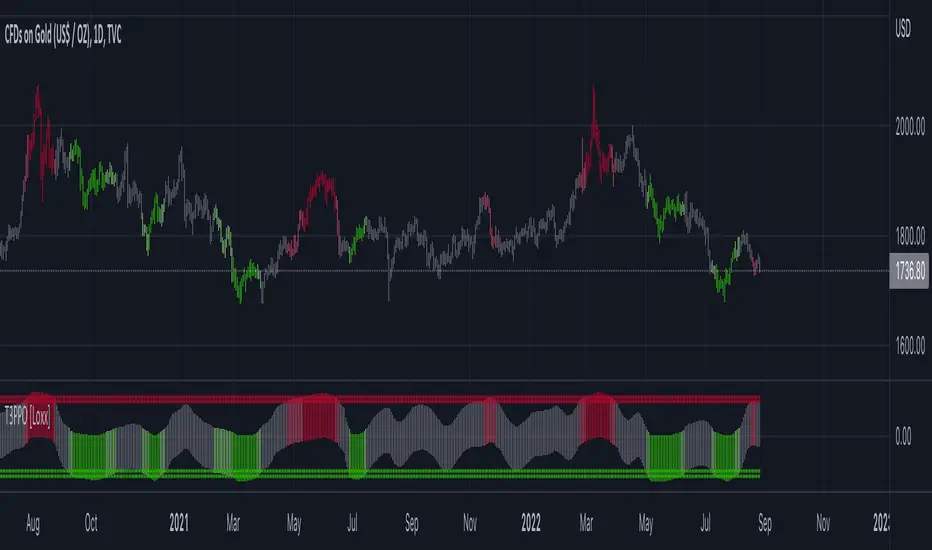
T3 PPO [Loxx]T3 PPO is a percentage price oscillator indicator using T3 moving average. This indicator is used to spot reversals. Dark red is upward price exhaustion, dark green is downward price exhaustion.
What is Percentage Price Oscillator (PPO)?
The percentage price oscillator (PPO) is a technical momentum indicator that shows the relationship between two moving averages in percentage terms. The moving averages are a 26-period and 12-period exponential moving average (EMA).
The PPO is used to compare asset performance and volatility, spot divergence that could lead to price reversals, generate trade signals, and help confirm trend direction.
What is the T3 moving average?
Better Moving Averages Tim Tillson
November 1, 1998
Tim Tillson is a software project manager at Hewlett-Packard, with degrees in Mathematics and Computer Science. He has privately traded options and equities for 15 years.
Introduction
"Digital filtering includes the process of smoothing, predicting, differentiating, integrating, separation of signals, and removal of noise from a signal. Thus many people who do such things are actually using digital filters without realizing that they are; being unacquainted with the theory, they neither understand what they have done nor the possibilities of what they might have done."
This quote from R. W. Hamming applies to the vast majority of indicators in technical analysis . Moving averages, be they simple, weighted, or exponential, are lowpass filters; low frequency components in the signal pass through with little attenuation, while high frequencies are severely reduced.
"Oscillator" type indicators (such as MACD , Momentum, Relative Strength Index ) are another type of digital filter called a differentiator.
Tushar Chande has observed that many popular oscillators are highly correlated, which is sensible because they are trying to measure the rate of change of the underlying time series, i.e., are trying to be the first and second derivatives we all learned about in Calculus.
We use moving averages (lowpass filters) in technical analysis to remove the random noise from a time series, to discern the underlying trend or to determine prices at which we will take action. A perfect moving average would have two attributes:
It would be smooth, not sensitive to random noise in the underlying time series. Another way of saying this is that its derivative would not spuriously alternate between positive and negative values.
It would not lag behind the time series it is computed from. Lag, of course, produces late buy or sell signals that kill profits.
The only way one can compute a perfect moving average is to have knowledge of the future, and if we had that, we would buy one lottery ticket a week rather than trade!
Having said this, we can still improve on the conventional simple, weighted, or exponential moving averages. Here's how:
Two Interesting Moving Averages
We will examine two benchmark moving averages based on Linear Regression analysis.
In both cases, a Linear Regression line of length n is fitted to price data.
I call the first moving average ILRS, which stands for Integral of Linear Regression Slope. One simply integrates the slope of a linear regression line as it is successively fitted in a moving window of length n across the data, with the constant of integration being a simple moving average of the first n points. Put another way, the derivative of ILRS is the linear regression slope. Note that ILRS is not the same as a SMA ( simple moving average ) of length n, which is actually the midpoint of the linear regression line as it moves across the data.
We can measure the lag of moving averages with respect to a linear trend by computing how they behave when the input is a line with unit slope. Both SMA (n) and ILRS(n) have lag of n/2, but ILRS is much smoother than SMA .
Our second benchmark moving average is well known, called EPMA or End Point Moving Average. It is the endpoint of the linear regression line of length n as it is fitted across the data. EPMA hugs the data more closely than a simple or exponential moving average of the same length. The price we pay for this is that it is much noisier (less smooth) than ILRS, and it also has the annoying property that it overshoots the data when linear trends are present.
However, EPMA has a lag of 0 with respect to linear input! This makes sense because a linear regression line will fit linear input perfectly, and the endpoint of the LR line will be on the input line.
These two moving averages frame the tradeoffs that we are facing. On one extreme we have ILRS, which is very smooth and has considerable phase lag. EPMA has 0 phase lag, but is too noisy and overshoots. We would like to construct a better moving average which is as smooth as ILRS, but runs closer to where EPMA lies, without the overshoot.
A easy way to attempt this is to split the difference, i.e. use (ILRS(n)+EPMA(n))/2. This will give us a moving average (call it IE /2) which runs in between the two, has phase lag of n/4 but still inherits considerable noise from EPMA. IE /2 is inspirational, however. Can we build something that is comparable, but smoother? Figure 1 shows ILRS, EPMA, and IE /2.
Filter Techniques
Any thoughtful student of filter theory (or resolute experimenter) will have noticed that you can improve the smoothness of a filter by running it through itself multiple times, at the cost of increasing phase lag.
There is a complementary technique (called twicing by J.W. Tukey) which can be used to improve phase lag. If L stands for the operation of running data through a low pass filter, then twicing can be described by:
L' = L(time series) + L(time series - L(time series))
That is, we add a moving average of the difference between the input and the moving average to the moving average. This is algebraically equivalent to:
2L-L(L)
This is the Double Exponential Moving Average or DEMA , popularized by Patrick Mulloy in TASAC (January/February 1994).
In our taxonomy, DEMA has some phase lag (although it exponentially approaches 0) and is somewhat noisy, comparable to IE /2 indicator.
We will use these two techniques to construct our better moving average, after we explore the first one a little more closely.
Fixing Overshoot
An n-day EMA has smoothing constant alpha=2/(n+1) and a lag of (n-1)/2.
Thus EMA (3) has lag 1, and EMA (11) has lag 5. Figure 2 shows that, if I am willing to incur 5 days of lag, I get a smoother moving average if I run EMA (3) through itself 5 times than if I just take EMA (11) once.
This suggests that if EPMA and DEMA have 0 or low lag, why not run fast versions (eg DEMA (3)) through themselves many times to achieve a smooth result? The problem is that multiple runs though these filters increase their tendency to overshoot the data, giving an unusable result. This is because the amplitude response of DEMA and EPMA is greater than 1 at certain frequencies, giving a gain of much greater than 1 at these frequencies when run though themselves multiple times. Figure 3 shows DEMA (7) and EPMA(7) run through themselves 3 times. DEMA^3 has serious overshoot, and EPMA^3 is terrible.
The solution to the overshoot problem is to recall what we are doing with twicing:
DEMA (n) = EMA (n) + EMA (time series - EMA (n))
The second term is adding, in effect, a smooth version of the derivative to the EMA to achieve DEMA . The derivative term determines how hot the moving average's response to linear trends will be. We need to simply turn down the volume to achieve our basic building block:
EMA (n) + EMA (time series - EMA (n))*.7;
This is algebraically the same as:
EMA (n)*1.7-EMA( EMA (n))*.7;
I have chosen .7 as my volume factor, but the general formula (which I call "Generalized Dema") is:
GD (n,v) = EMA (n)*(1+v)-EMA( EMA (n))*v,
Where v ranges between 0 and 1. When v=0, GD is just an EMA , and when v=1, GD is DEMA . In between, GD is a cooler DEMA . By using a value for v less than 1 (I like .7), we cure the multiple DEMA overshoot problem, at the cost of accepting some additional phase delay. Now we can run GD through itself multiple times to define a new, smoother moving average T3 that does not overshoot the data:
T3(n) = GD ( GD ( GD (n)))
In filter theory parlance, T3 is a six-pole non-linear Kalman filter. Kalman filters are ones which use the error (in this case (time series - EMA (n)) to correct themselves. In Technical Analysis , these are called Adaptive Moving Averages; they track the time series more aggressively when it is making large moves.
Mean-Reversion with CooldownThis strategy requires no indicators or fundamental analysis. It is designed for longer-term positions and works especially well on unleveraged instruments with strong long-term upward trends, such as precious metals. Feel free to experiment with different timeframes — I’ve found that 1-hour charts work particularly well for cryptocurrencies.
The idea is to filter out ongoing bear phases as effectively as possible and capitalize on long-term bull runs.
The script implements an idea that came to me in a state of complete sleep deprivation: open a random long position with a fixed take-profit (TP) and a tight stop-loss (SL).
If the TP is hit — great, we simply try again.
If the SL is triggered — too bad, we pause for a while and then try again.
## Cooldown (Waiting) Mechanism
The waiting mechanism is simple: the more consecutive SL hits we get, the longer we wait before opening the next trade. The waiting time is measured in closed candles, and thus depends on the timeframe you are using.
## Two cooldown calculation modes are currently supported:
### 1. FIBONACCI
The cooldown follows the Fibonacci sequence, based on the number of consecutive losses:
1st loss → wait 1 bar
2nd loss → wait 1 bar
3rd loss → wait 2 or 3 bars (depending on definition)
4th loss → wait 3 or 5 bars
etc.
### 2. POWER OF TWO
The cooldown increases exponentially:
1st loss → wait 2 bars
2nd loss → wait 4 bars
3rd loss → wait 8 bars
4th loss → wait 16 bars
and so on, using the formula 2ⁿ.
## Configurable Parameters
### Cooldown Pause Calculation
The settings allow you to define the SL and TP as percentages of the position value.
The "Cooldown Pause Calculation" option determines how the next cooldown duration is computed after a losing trade.
The system keeps track of how many consecutive losses have occurred since the last profitable trade. That counter is then used to compute how many bars we must wait before opening the next position.
### Maximum Cooldown
The "Max Cooldown Candles" setting defines the maximum number of bars we are allowed to wait before placing a new trade. This prevents the strategy from “locking itself out” for too long and mitigates the fear of missing out (FOMO).
Once the cooldown duration reaches this maximum, the system essentially wraps around and starts the progression again. In the script, this is handled using a simple modulo operation based on the chosen maximum.

Algorithm Predator - ML-liteAlgorithm Predator - ML-lite
This indicator combines four specialized trading agents with an adaptive multi-armed bandit selection system to identify high-probability trade setups. It is designed for swing and intraday traders who want systematic signal generation based on institutional order flow patterns , momentum exhaustion , liquidity dynamics , and statistical mean reversion .
Core Architecture
Why These Components Are Combined:
The script addresses a fundamental challenge in algorithmic trading: no single detection method works consistently across all market conditions. By deploying four independent agents and using reinforcement learning algorithms to select or blend their outputs, the system adapts to changing market regimes without manual intervention.
The Four Trading Agents
1. Spoofing Detector Agent 🎭
Detects iceberg orders through persistent volume at similar price levels over 5 bars
Identifies spoofing patterns via asymmetric wick analysis (wicks exceeding 60% of bar range with volume >1.8× average)
Monitors order clustering using simplified Hawkes process intensity tracking (exponential decay model)
Signal Logic: Contrarian—fades false breakouts caused by institutional manipulation
Best Markets: Consolidations, institutional trading windows, low-liquidity hours
2. Exhaustion Detector Agent ⚡
Calculates RSI divergence between price movement and momentum indicator over 5-bar window
Detects VWAP exhaustion (price at 2σ bands with declining volume)
Uses VPIN reversals (volume-based toxic flow dissipation) to identify momentum failure
Signal Logic: Counter-trend—enters when momentum extreme shows weakness
Best Markets: Trending markets reaching climax points, over-extended moves
3. Liquidity Void Detector Agent 💧
Measures Bollinger Band squeeze (width <60% of 50-period average)
Identifies stop hunts via 20-bar high/low penetration with immediate reversal and volume spike
Detects hidden liquidity absorption (volume >2× average with range <0.3× ATR)
Signal Logic: Breakout anticipation—enters after liquidity grab but before main move
Best Markets: Range-bound pre-breakout, volatility compression zones
4. Mean Reversion Agent 📊
Calculates price z-scores relative to 50-period SMA and standard deviation (triggers at ±2σ)
Implements Ornstein-Uhlenbeck process scoring (mean-reverting stochastic model)
Uses entropy analysis to detect algorithmic trading patterns (low entropy <0.25 = high predictability)
Signal Logic: Statistical reversion—enters when price deviates significantly from statistical equilibrium
Best Markets: Range-bound, low-volatility, algorithmically-dominated instruments
Adaptive Selection: Multi-Armed Bandit System
The script implements four reinforcement learning algorithms to dynamically select or blend agents based on performance:
Thompson Sampling (Default - Recommended):
Uses Bayesian inference with beta distributions (tracks alpha/beta parameters per agent)
Balances exploration (trying underused agents) vs. exploitation (using proven winners)
Each agent's win/loss history informs its selection probability
Lite Approximation: Uses pseudo-random sampling from price/volume noise instead of true random number generation
UCB1 (Upper Confidence Bound):
Calculates confidence intervals using: average_reward + sqrt(2 × ln(total_pulls) / agent_pulls)
Deterministic algorithm favoring agents with high uncertainty (potential upside)
More conservative than Thompson Sampling
Epsilon-Greedy:
Exploits best-performing agent (1-ε)% of the time
Explores randomly ε% of the time (default 10%, configurable 1-50%)
Simple, transparent, easily tuned via epsilon parameter
Gradient Bandit:
Uses softmax probability distribution over agent preference weights
Updates weights via gradient ascent based on rewards
Best for Blend mode where all agents contribute
Selection Modes:
Switch Mode: Uses only the selected agent's signal (clean, decisive)
Blend Mode: Combines all agents using exponentially weighted confidence scores controlled by temperature parameter (smooth, diversified)
Lock Agent Feature:
Optional manual override to force one specific agent
Useful after identifying which agent dominates your specific instrument
Only applies in Switch mode
Four choices: Spoofing Detector, Exhaustion Detector, Liquidity Void, Mean Reversion
Memory System
Dual-Layer Architecture:
Short-Term Memory: Stores last 20 trade outcomes per agent (configurable 10-50)
Long-Term Memory: Stores episode averages when short-term reaches transfer threshold (configurable 5-20 bars)
Memory Boost Mechanism: Recent performance modulates agent scores by up to ±20%
Episode Transfer: When an agent accumulates sufficient results, averages are condensed into long-term storage
Persistence: Manual restoration of learned parameters via input fields (alpha, beta, weights, microstructure thresholds)
How Memory Works:
Agent generates signal → outcome tracked after 8 bars (performance horizon)
Result stored in short-term memory (win = 1.0, loss = 0.0)
Short-term average influences agent's future scores (positive feedback loop)
After threshold met (default 10 results), episode averaged into long-term storage
Long-term patterns (weighted 30%) + short-term patterns (weighted 70%) = total memory boost
Market Microstructure Analysis
These advanced metrics quantify institutional order flow dynamics:
Order Flow Toxicity (Simplified VPIN):
Measures buy/sell volume imbalance over 20 bars: |buy_vol - sell_vol| / (buy_vol + sell_vol)
Detects informed trading activity (institutional players with non-public information)
Values >0.4 indicate "toxic flow" (informed traders active)
Lite Approximation: Uses simple open/close heuristic instead of tick-by-tick trade classification
Price Impact Analysis (Simplified Kyle's Lambda):
Measures market impact efficiency: |price_change_10| / sqrt(volume_sum_10)
Low values = large orders with minimal price impact ( stealth accumulation )
High values = retail-dominated moves with high slippage
Lite Approximation: Uses simplified denominator instead of regression-based signed order flow
Market Randomness (Entropy Analysis):
Counts unique price changes over 20 bars / 20
Measures market predictability
High entropy (>0.6) = human-driven, chaotic price action
Low entropy (<0.25) = algorithmic trading dominance (predictable patterns)
Lite Approximation: Simple ratio instead of true Shannon entropy H(X) = -Σ p(x)·log₂(p(x))
Order Clustering (Simplified Hawkes Process):
Tracks self-exciting event intensity (coordinated order activity)
Decays at 0.9× per bar, spikes +1.0 when volume >1.5× average
High intensity (>0.7) indicates clustering (potential spoofing/accumulation)
Lite Approximation: Simple exponential decay instead of full λ(t) = μ + Σ α·exp(-β(t-tᵢ)) with MLE
Signal Generation Process
Multi-Stage Validation:
Stage 1: Agent Scoring
Each agent calculates internal score based on its detection criteria
Scores must exceed agent-specific threshold (adjusted by sensitivity multiplier)
Agent outputs: Signal direction (+1/-1/0) and Confidence level (0.0-1.0)
Stage 2: Memory Boost
Agent scores multiplied by memory boost factor (0.8-1.2 based on recent performance)
Successful agents get amplified, failing agents get dampened
Stage 3: Bandit Selection/Blending
If Adaptive Mode ON:
Switch: Bandit selects single best agent, uses only its signal
Blend: All agents combined using softmax-weighted confidence scores
If Adaptive Mode OFF:
Traditional consensus voting with confidence-squared weighting
Signal fires when consensus exceeds threshold (default 70%)
Stage 4: Confirmation Filter
Raw signal must repeat for consecutive bars (default 3, configurable 2-4)
Minimum confidence threshold: 0.25 (25%) enforced regardless of mode
Trend alignment check: Long signals require trend_score ≥ -2, Short signals require trend_score ≤ 2
Stage 5: Cooldown Enforcement
Minimum bars between signals (default 10, configurable 5-15)
Prevents over-trading during choppy conditions
Stage 6: Performance Tracking
After 8 bars (performance horizon), signal outcome evaluated
Win = price moved in signal direction, Loss = price moved against
Results fed back into memory and bandit statistics
Trading Modes (Presets)
Pre-configured parameter sets:
Conservative: 85% consensus, 4 confirmations, 15-bar cooldown
Expected: 60-70% win rate, 3-8 signals/week
Best for: Swing trading, capital preservation, beginners
Balanced: 70% consensus, 3 confirmations, 10-bar cooldown
Expected: 55-65% win rate, 8-15 signals/week
Best for: Day trading, most traders, general use
Aggressive: 60% consensus, 2 confirmations, 5-bar cooldown
Expected: 50-58% win rate, 15-30 signals/week
Best for: Scalping, high-frequency trading, active management
Elite: 75% consensus, 3 confirmations, 12-bar cooldown
Expected: 58-68% win rate, 5-12 signals/week
Best for: Selective trading, high-conviction setups
Adaptive: 65% consensus, 2 confirmations, 8-bar cooldown
Expected: Varies based on learning
Best for: Experienced users leveraging bandit system
How to Use
1. Initial Setup (5 Minutes):
Select Trading Mode matching your style (start with Balanced)
Enable Adaptive Learning (recommended for automatic agent selection)
Choose Thompson Sampling algorithm (best all-around performance)
Keep Microstructure Metrics enabled for liquid instruments (>100k daily volume)
2. Agent Tuning (Optional):
Adjust Agent Sensitivity multipliers (0.5-2.0):
<0.8 = Highly selective (fewer signals, higher quality)
0.9-1.2 = Balanced (recommended starting point)
1.3 = Aggressive (more signals, lower individual quality)
Monitor dashboard for 20-30 signals to identify dominant agent
If one agent consistently outperforms, consider using Lock Agent feature
3. Bandit Configuration (Advanced):
Blend Temperature (0.1-2.0):
0.3 = Sharp decisions (best agent dominates)
0.5 = Balanced (default)
1.0+ = Smooth (equal weighting, democratic)
Memory Decay (0.8-0.99):
0.90 = Fast adaptation (volatile markets)
0.95 = Balanced (most instruments)
0.97+ = Long memory (stable trends)
4. Signal Interpretation:
Green triangle (▲): Long signal confirmed
Red triangle (▼): Short signal confirmed
Dashboard shows:
Active agent (highlighted row with ► marker)
Win rate per agent (green >60%, yellow 40-60%, red <40%)
Confidence bars (█████ = maximum confidence)
Memory size (short-term buffer count)
Colored zones display:
Entry level (current close)
Stop-loss (1.5× ATR)
Take-profit 1 (2.0× ATR)
Take-profit 2 (3.5× ATR)
5. Risk Management:
Never risk >1-2% per signal (use ATR-based stops)
Signals are entry triggers, not complete strategies
Combine with your own market context analysis
Consider fundamental catalysts and news events
Use "Confirming" status to prepare entries (not to enter early)
6. Memory Persistence (Optional):
After 50-100 trades, check Memory Export Panel
Record displayed alpha/beta/weight values for each agent
Record VPIN and Kyle threshold values
Enable "Restore From Memory" and input saved values to continue learning
Useful when switching timeframes or restarting indicator
Visual Components
On-Chart Elements:
Spectral Layers: EMA8 ± 0.5 ATR bands (dynamic support/resistance, colored by trend)
Energy Radiance: Multi-layer glow boxes at signal points (intensity scales with confidence, configurable 1-5 layers)
Probability Cones: Projected price paths with uncertainty wedges (15-bar projection, width = confidence × ATR)
Connection Lines: Links sequential signals (solid = same direction continuation, dotted = reversal)
Kill Zones: Risk/reward boxes showing entry, stop-loss, and dual take-profit targets
Signal Markers: Triangle up/down at validated entry points
Dashboard (Configurable Position & Size):
Regime Indicator: 4-level trend classification (Strong Bull/Bear, Weak Bull/Bear)
Mode Status: Shows active system (Adaptive Blend, Locked Agent, or Consensus)
Agent Performance Table: Real-time win%, confidence, and memory stats
Order Flow Metrics: Toxicity and impact indicators (when microstructure enabled)
Signal Status: Current state (Long/Short/Confirming/Waiting) with confirmation progress
Memory Panel (Configurable Position & Size):
Live Parameter Export: Alpha, beta, and weight values per agent
Adaptive Thresholds: Current VPIN sensitivity and Kyle threshold
Save Reminder: Visual indicator if parameters should be recorded
What Makes This Original
This script's originality lies in three key innovations:
1. Genuine Meta-Learning Framework:
Unlike traditional indicator mashups that simply display multiple signals, this implements authentic reinforcement learning (multi-armed bandits) to learn which detection method works best in current conditions. The Thompson Sampling implementation with beta distribution tracking (alpha for successes, beta for failures) is statistically rigorous and adapts continuously. This is not post-hoc optimization—it's real-time learning.
2. Episodic Memory Architecture with Transfer Learning:
The dual-layer memory system mimics human learning patterns:
Short-term memory captures recent performance (recency bias)
Long-term memory preserves historical patterns (experience)
Automatic transfer mechanism consolidates knowledge
Memory boost creates positive feedback loops (successful strategies become stronger)
This architecture allows the system to adapt without retraining , unlike static ML models that require batch updates.
3. Institutional Microstructure Integration:
Combines retail-focused technical analysis (RSI, Bollinger Bands, VWAP) with institutional-grade microstructure metrics (VPIN, Kyle's Lambda, Hawkes processes) typically found in academic finance literature and professional trading systems, not standard retail platforms. While simplified for Pine Script constraints, these metrics provide insight into informed vs. uninformed trading , a dimension entirely absent from traditional technical analysis.
Mashup Justification:
The four agents are combined specifically for risk diversification across failure modes:
Spoofing Detector: Prevents false breakout losses from manipulation
Exhaustion Detector: Prevents chasing extended trends into reversals
Liquidity Void: Exploits volatility compression (different regime than trending)
Mean Reversion: Provides mathematical anchoring when patterns fail
The bandit system ensures the optimal tool is automatically selected for each market situation, rather than requiring manual interpretation of conflicting signals.
Why "ML-lite"? Simplifications and Approximations
This is the "lite" version due to necessary simplifications for Pine Script execution:
1. Simplified VPIN Calculation:
Academic Implementation: True VPIN uses volume bucketing (fixed-volume bars) and tick-by-tick buy/sell classification via Lee-Ready algorithm or exchange-provided trade direction flags
This Implementation: 20-bar rolling window with simple open/close heuristic (close > open = buy volume)
Impact: May misclassify volume during ranging/choppy markets; works best in directional moves
2. Pseudo-Random Sampling:
Academic Implementation: Thompson Sampling requires true random number generation from beta distributions using inverse transform sampling or acceptance-rejection methods
This Implementation: Deterministic pseudo-randomness derived from price and volume decimal digits: (close × 100 - floor(close × 100)) + (volume % 100) / 100
Impact: Not cryptographically random; may have subtle biases in specific price ranges; provides sufficient variation for agent selection
3. Hawkes Process Approximation:
Academic Implementation: Full Hawkes process uses maximum likelihood estimation with exponential kernels: λ(t) = μ + Σ α·exp(-β(t-tᵢ)) fitted via iterative optimization
This Implementation: Simple exponential decay (0.9 multiplier) with binary event triggers (volume spike = event)
Impact: Captures self-exciting property but lacks parameter optimization; fixed decay rate may not suit all instruments
4. Kyle's Lambda Simplification:
Academic Implementation: Estimated via regression of price impact on signed order flow over multiple time intervals: Δp = λ × Δv + ε
This Implementation: Simplified ratio: price_change / sqrt(volume_sum) without proper signed order flow or regression
Impact: Provides directional indicator of impact but not true market depth measurement; no statistical confidence intervals
5. Entropy Calculation:
Academic Implementation: True Shannon entropy requires probability distribution: H(X) = -Σ p(x)·log₂(p(x)) where p(x) is probability of each price change magnitude
This Implementation: Simple ratio of unique price changes to total observations (variety measure)
Impact: Measures diversity but not true information entropy with probability weighting; less sensitive to distribution shape
6. Memory System Constraints:
Full ML Implementation: Neural networks with backpropagation, experience replay buffers (storing state-action-reward tuples), gradient descent optimization, and eligibility traces
This Implementation: Fixed-size array queues with simple averaging; no gradient-based learning, no state representation beyond raw scores
Impact: Cannot learn complex non-linear patterns; limited to linear performance tracking
7. Limited Feature Engineering:
Advanced Implementation: Dozens of engineered features, polynomial interactions (x², x³), dimensionality reduction (PCA, autoencoders), feature selection algorithms
This Implementation: Raw agent scores and basic market metrics (RSI, ATR, volume ratio); minimal transformation
Impact: May miss subtle cross-feature interactions; relies on agent-level intelligence rather than feature combinations
8. Single-Instrument Data:
Full Implementation: Multi-asset correlation analysis (sector ETFs, currency pairs, volatility indices like VIX), lead-lag relationships, risk-on/risk-off regimes
This Implementation: Only OHLCV data from displayed instrument
Impact: Cannot incorporate broader market context; vulnerable to correlated moves across assets
9. Fixed Performance Horizon:
Full Implementation: Adaptive horizon based on trade duration, volatility regime, or profit target achievement
This Implementation: Fixed 8-bar evaluation window
Impact: May evaluate too early in slow markets or too late in fast markets; one-size-fits-all approach
Performance Impact Summary:
These simplifications make the script:
✅ Faster: Executes in milliseconds vs. seconds (or minutes) for full academic implementations
✅ More Accessible: Runs on any TradingView plan without external data feeds, APIs, or compute servers
✅ More Transparent: All calculations visible in Pine Script (no black-box compiled models)
✅ Lower Resource Usage: <500 bars lookback, minimal memory footprint
⚠️ Less Precise: Approximations may reduce statistical edge by 5-15% vs. academic implementations
⚠️ Limited Scope: Cannot capture tick-level dynamics, multi-order-book interactions, or cross-asset flows
⚠️ Fixed Parameters: Some thresholds hardcoded rather than dynamically optimized
When to Upgrade to Full Implementation:
Consider professional Python/C++ versions with institutional data feeds if:
Trading with >$100K capital where precision differences materially impact returns
Operating in microsecond-competitive environments (HFT, market making)
Requiring regulatory-grade audit trails and reproducibility
Backtesting with tick-level precision for strategy validation
Need true real-time adaptation with neural network-based learning
For retail swing/day trading and position management, these approximations provide sufficient signal quality while maintaining usability, transparency, and accessibility. The core logic—multi-agent detection with adaptive selection—remains intact.
Technical Notes
All calculations use standard Pine Script built-in functions ( ta.ema, ta.atr, ta.rsi, ta.bb, ta.sma, ta.stdev, ta.vwap )
VPIN and Kyle's Lambda use simplified formulas optimized for OHLCV data (see "Lite" section above)
Thompson Sampling uses pseudo-random noise from price/volume decimal digits for beta distribution sampling
No repainting: All calculations use confirmed bar data (no forward-looking)
Maximum lookback: 500 bars (set via max_bars_back parameter)
Performance evaluation: 8-bar forward-looking window for reward calculation (clearly disclosed)
Confidence threshold: Minimum 0.25 (25%) enforced on all signals
Memory arrays: Dynamic sizing with FIFO queue management
Limitations and Disclaimers
Not Predictive: This indicator identifies patterns in historical data. It cannot predict future price movements with certainty.
Requires Human Judgment: Signals are entry triggers, not complete trading strategies. Must be confirmed with your own analysis, risk management rules, and market context.
Learning Period Required: The adaptive system requires 50-100 bars minimum to build statistically meaningful performance data for bandit algorithms.
Overfitting Risk: Restoring memory parameters from one market regime to a drastically different regime (e.g., low volatility to high volatility) may cause poor initial performance until system re-adapts.
Approximation Limitations: Simplified calculations (see "Lite" section) may underperform academic implementations by 5-15% in highly efficient markets.
No Guarantee of Profit: Past performance, whether backtested or live-traded, does not guarantee future performance. All trading involves risk of loss.
Forward-Looking Bias: Performance evaluation uses 8-bar forward window—this creates slight look-ahead for learning (though not for signals). Real-time performance may differ from indicator's internal statistics.
Single-Instrument Limitation: Does not account for correlations with related assets or broader market regime changes.
Recommended Settings
Timeframe: 15-minute to 4-hour charts (sufficient volatility for ATR-based stops; adequate bar volume for learning)
Assets: Liquid instruments with >100k daily volume (forex majors, large-cap stocks, BTC/ETH, major indices)
Not Recommended: Illiquid small-caps, penny stocks, low-volume altcoins (microstructure metrics unreliable)
Complementary Tools: Volume profile, order book depth, market breadth indicators, fundamental catalysts
Position Sizing: Risk no more than 1-2% of capital per signal using ATR-based stop-loss
Signal Filtering: Consider external confluence (support/resistance, trendlines, round numbers, session opens)
Start With: Balanced mode, Thompson Sampling, Blend mode, default agent sensitivities (1.0)
After 30+ Signals: Review agent win rates, consider increasing sensitivity of top performers or locking to dominant agent
Alert Configuration
The script includes built-in alert conditions:
Long Signal: Fires when validated long entry confirmed
Short Signal: Fires when validated short entry confirmed
Alerts fire once per bar (after confirmation requirements met)
Set alert to "Once Per Bar Close" for reliability
Taking you to school. — Dskyz, Trade with insight. Trade with anticipation.

Auto-Fit Growth Trendline# **Theoretical Algorithmic Principles of the Auto-Fit Growth Trendline (AFGT)**
## **🎯 What Does This Algorithm Do?**
The Auto-Fit Growth Trendline is an advanced technical analysis system that **automates the identification of long-term growth trends** and **projects future price levels** based on historical cyclical patterns.
### **Primary Functionality:**
- **Automatically detects** the most significant lows in regular periods (monthly, quarterly, semi-annually, annually)
- **Constructs a dynamic trendline** that connects these historical lows
- **Projects the trend into the future** with high mathematical precision
- **Generates Fibonacci bands** that act as dynamic support and resistance levels
- **Automatically adapts** to different timeframes and market conditions
### **Strategic Purpose:**
The algorithm is designed to identify **fundamental value zones** where price has historically found support, enabling traders to:
- Identify optimal entry points for long positions
- Establish realistic price targets based on mathematical projections
- Recognize dynamic support and resistance levels
- Anticipate long-term price movements
---
## **🧮 Core Mathematical Foundations**
### **Adaptive Temporal Segmentation Theory**
The algorithm is based on **dynamic temporal partition theory**, where time is divided into mathematically coherent uniform intervals. It uses modular transformations to create bijective mappings between continuous timestamps and discrete periods, ensuring each temporal point belongs uniquely to a specific period.
**What does this achieve?** It allows the algorithm to automatically identify natural market cycles (annual, quarterly, etc.) without manual intervention, adapting to the inherent periodicity of each asset.
The temporal mapping function implements a **discrete affine transformation** that normalizes different frequencies (monthly, quarterly, semi-annual, annual) to a space of unique identifiers, enabling consistent cross-temporal comparative analysis.
---
## **📊 Local Extrema Detection Theory**
### **Multi-Point Retrospective Validation Principle**
Local minima detection is founded on **relative extrema theory with sliding window**. Instead of using a simple minimum finder, it implements a cross-validation system that examines the persistence of the extremum across multiple historical periods.
**What problem does this solve?** It eliminates false minima caused by temporal volatility, identifying only those points that represent true historical support levels with statistical significance.
This approach is based on the **statistical confirmation principle**, where a minimum is only considered valid if it maintains its extremum condition during a defined observation period, significantly reducing false positives caused by transitory volatility.
---
## **🔬 Robust Interpolation Theory with Outlier Control**
### **Contextual Adaptive Interpolation Model**
The mathematical core uses **piecewise linear interpolation with adaptive outlier correction**. The key innovation lies in implementing a **contextual anomaly detector** that identifies not only absolute extreme values, but relative deviations to the local context.
**Why is this important?** Financial markets contain extreme events (crashes, bubbles) that can distort projections. This system identifies and appropriately weights them without completely eliminating them, preserving directional information while attenuating distortions.
### **Implicit Bayesian Smoothing Algorithm**
When an outlier is detected (deviation >300% of local average), the system applies a **simplified Kalman filter** that combines the current observation with a local trend estimation, using a weight factor that preserves directional information while attenuating extreme fluctuations.
---
## **📈 Stabilized Extrapolation Theory**
### **Exponential Growth Model with Dampening**
Extrapolation is based on a **modified exponential growth model with progressive dampening**. It uses multiple historical points to calculate local growth ratios, implements statistical filtering to eliminate outliers, and applies a dampening factor that increases with extrapolation distance.
**What advantage does this offer?** Long-term projections in finance tend to be exponentially unrealistic. This system maintains short-to-medium term accuracy while converging toward realistic long-term projections, avoiding the typical "exponential explosions" of other methods.
### **Asymptotic Convergence Principle**
For long-term projections, the algorithm implements **controlled asymptotic convergence**, where growth ratios gradually converge toward pre-established limits, avoiding unrealistic exponential projections while preserving short-to-medium term accuracy.
---
## **🌟 Dynamic Fibonacci Projection Theory**
### **Continuous Proportional Scaling Model**
Fibonacci bands are constructed through **uniform proportional scaling** of the base curve, where each level represents a linear transformation of the main curve by a constant factor derived from the Fibonacci sequence.
**What is its practical utility?** It provides dynamic resistance and support levels that move with the trend, offering price targets and profit-taking points that automatically adapt to market evolution.
### **Topological Preservation Principle**
The system maintains the **topological properties** of the base curve in all Fibonacci projections, ensuring that spatial and temporal relationships are consistently preserved across all resistance/support levels.
---
## **⚡ Adaptive Computational Optimization**
### **Multi-Scale Resolution Theory**
It implements **automatic multi-resolution analysis** where data granularity is dynamically adjusted according to the analysis timeframe. It uses the **adaptive Nyquist principle** to optimize the signal-to-noise ratio according to the temporal observation scale.
**Why is this necessary?** Different timeframes require different levels of detail. A 1-minute chart needs more granularity than a monthly one. This system automatically optimizes resolution for each case.
### **Adaptive Density Algorithm**
Calculation point density is optimized through **adaptive sampling theory**, where calculation frequency is adjusted according to local trend curvature and analysis timeframe, balancing visual precision with computational efficiency.
---
## **🛡️ Robustness and Fault Tolerance**
### **Graceful Degradation Theory**
The system implements **multi-level graceful degradation**, where under error conditions or insufficient data, the algorithm progressively falls back to simpler but reliable methods, maintaining basic functionality under any condition.
**What does this guarantee?** That the indicator functions consistently even with incomplete data, new symbols with limited history, or extreme market conditions.
### **State Consistency Principle**
It uses **mathematical invariants** to guarantee that the algorithm's internal state remains consistent between executions, implementing consistency checks that validate data structure integrity in each iteration.
---
## **🔍 Key Theoretical Innovations**
### **A. Contextual vs. Absolute Outlier Detection**
It revolutionizes traditional outlier detection by considering not only the absolute magnitude of deviations, but their relative significance within the local context of the time series.
**Practical impact:** It distinguishes between legitimate market movements and technical anomalies, preserving important events like breakouts while filtering noise.
### **B. Extrapolation with Weighted Historical Memory**
It implements a memory system that weights different historical periods according to their relevance for current prediction, creating projections more adaptable to market regime changes.
**Competitive advantage:** It automatically adapts to fundamental changes in asset dynamics without requiring manual recalibration.
### **C. Automatic Multi-Timeframe Adaptation**
It develops an automatic temporal resolution selection system that optimizes signal extraction according to the intrinsic characteristics of the analysis timeframe.
**Result:** A single indicator that functions optimally from 1-minute to monthly charts without manual adjustments.
### **D. Intelligent Asymptotic Convergence**
It introduces the concept of controlled asymptotic convergence in financial extrapolations, where long-term projections converge toward realistic limits based on historical fundamentals.
**Added value:** Mathematically sound long-term projections that avoid the unrealistic extremes typical of other extrapolation methods.
---
## **📊 Complexity and Scalability Theory**
### **Optimized Linear Complexity Model**
The algorithm maintains **linear computational complexity** O(n) in the number of historical data points, guaranteeing scalability for extensive time series analysis without performance degradation.
### **Temporal Locality Principle**
It implements **temporal locality**, where the most expensive operations are concentrated in the most relevant temporal regions (recent periods and near projections), optimizing computational resource usage.
---
## **🎯 Convergence and Stability**
### **Probabilistic Convergence Theory**
The system guarantees **probabilistic convergence** toward the real underlying trend, where projection accuracy increases with the amount of available historical data, following **law of large numbers** principles.
**Practical implication:** The more history an asset has, the more accurate the algorithm's projections will be.
### **Guaranteed Numerical Stability**
It implements **intrinsic numerical stability** through the use of robust floating-point arithmetic and validations that prevent overflow, underflow, and numerical error propagation.
**Result:** Reliable operation even with extreme-priced assets (from satoshis to thousand-dollar stocks).
---
## **💼 Comprehensive Practical Application**
**The algorithm functions as a "financial GPS"** that:
1. **Identifies where we've been** (significant historical lows)
2. **Determines where we are** (current position relative to the trend)
3. **Projects where we're going** (future trend with specific price levels)
4. **Provides alternative routes** (Fibonacci bands as alternative targets)
This theoretical framework represents an innovative synthesis of time series analysis, approximation theory, and computational optimization, specifically designed for long-term financial trend analysis with robust and mathematically grounded projections.
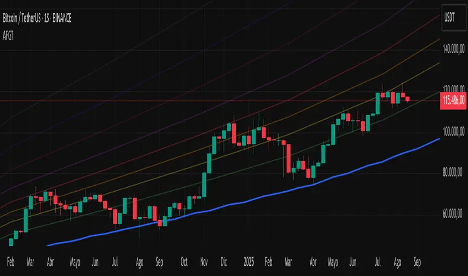
remaLibrary " REMA "
Custom Regional Exponential Moving Average with enhanced sensitivity to recent price action
Description: What Makes REMA Unique?
REMA introduces a dual-region weighting system that intelligently balances short-term responsiveness with long-term trend context, solving the fundamental limitation of standard EMAs where longer periods necessarily sacrifice recent price sensitivity.
Key Differences from Standard EMA:
Adaptive Regional Weighting: Applies stronger exponential decay to recent price data while maintaining appropriate weighting for historical context.
Maintains Responsiveness at Any Length: Unlike standard EMAs where longer periods become progressively less responsive, REMA preserves significant sensitivity to recent price action even at 100+ period lengths.
Mathematically Sound Enhancement: Preserves the core mathematical integrity of exponential averaging while introducing region-specific weighting that better reflects how traders actually interpret price action.
Value to TradingView Community:
Improved Signal Timing: Detects reversals 1-3 bars earlier than traditional EMAs without increasing false signals.
Better Multi-Timeframe Analysis: Provides more consistent behavior across different period settings, reducing conflicting signals between timeframes.
Ideal for Modern Markets: Better handles today's high-volatility, algorithm-driven markets where traditional indicators often lag too much to be effective.
Optimized for Both Trend and Reversal Trading: Simultaneously provides strong trend-following capabilities while remaining sensitive to legitimate reversal signals.
Computation Efficiency: The fast implementation offers enhanced capabilities with minimal computational overhead, making it practical for real-time analysis.
REMA fills a critical gap between lagging long-period EMAs and noisy short-period EMAs, giving traders a single, versatile tool that adapts to market conditions more effectively than standard technical indicators.
Implementation:
rema(src, length, recency_bias, transition_point)
Regional Exponential Moving Average that maintains recent price sensitivity even with long lookback periods
Parameters:
src (float) : Input source series
length (int) : Overall EMA period length
recency_bias (float) : Weighting factor to increase sensitivity to recent prices (1.0-3.0 recommended)
transition_point (float) : Percentage point (0.0-1.0) in the lookback period where weighting shifts from recent to historical
Returns: Custom exponentially weighted moving average with regional bias
rema_fast(src, length, recency_bias)
Simplified Regional EMA that uses a recursive calculation method
Parameters:
src (float) : Input source series
length (int) : Overall EMA period
recency_bias (float) : Factor to increase sensitivity to recent price (1.0-3.0 recommended)
Returns: Computationally efficient regional EMA
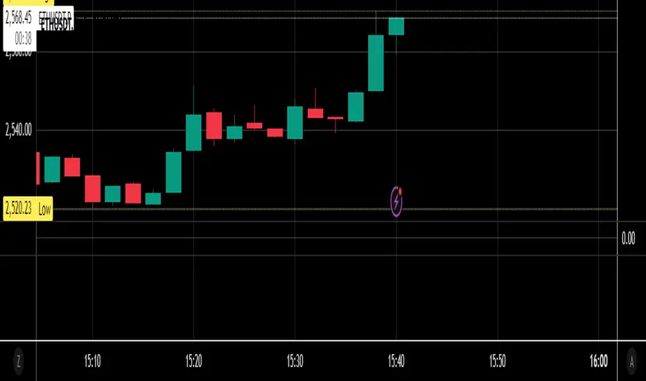
Uptrick: Acceleration ShiftsIntroduction
Uptrick: Acceleration Shifts is designed to measure and visualize price momentum shifts by focusing on acceleration —the rate of change in velocity over time. It uses various moving average techniques as a trend filter, providing traders with a clearer perspective on market direction and potential trade entries or exits.
Purpose
The main goal of this indicator is to spot strong momentum changes (accelerations) and confirm them with a chosen trend filter. It attempts to distinguish genuine market moves from noise, helping traders make more informed decisions. The script can also trigger multiple entries (smart pyramiding) within the same trend, if desired.
Overview
By measuring how quickly price velocity changes (acceleration) and comparing it against a smoothed average of itself, this script generates buy or sell signals once the acceleration surpasses a given threshold. A trend filter is added for further validation. Users can choose from multiple smoothing methods and color schemes, and they can optionally enable a small table that displays real-time acceleration values.
Originality and Uniqueness
This script offers an acceleration-based approach, backed by several different moving average choices. The blend of acceleration thresholds, a trend filter, and an optional extra-entry (pyramiding) feature provides a flexible toolkit for various trading styles. The inclusion of multiple color themes and a slope-based coloring of the trend line adds clarity and user customization.
Inputs & Features
1. Acceleration Length (length)
This input determines the number of bars used when calculating velocity. Specifically, the script computes velocity by taking the difference in closing prices over length bars, and then calculates acceleration based on how that velocity changes over an additional length. The default is 14.
2. Trend Filter Length (smoothing)
This sets the lookback period for the chosen trend filter method. The default of 50 results in a moderately smooth trend line. A higher smoothing value will create a slower-moving trend filter.
3. Acceleration Threshold (threshold)
This multiplier determines when acceleration is considered strong enough to trigger a main buy or sell signal. A default value of 2.5 means the current acceleration must exceed 2.5 times the average acceleration before signaling.
4. Smart Pyramiding Strength (pyramidingThreshold)
This lower threshold is used for additional (pyramiding) entries once the main trend has already been identified. For instance, if set to 0.5, the script looks for acceleration crossing ±0.5 times its average acceleration to add extra positions.
5. Max Pyramiding Entries (maxPyramidingEntries)
This sets a limit on how many extra positions can be opened (beyond the first main signal) in a single directional trend. The default of 3 ensures traders do not become overexposed.
6. Show Acceleration Table (showTable)
When enabled, a small table displaying the current acceleration and its average is added to the top-right corner of the chart. This table helps monitor real-time momentum changes.
7. Smart Pyramiding (enablePyramiding)
This toggle decides whether additional entries (buy or sell) will be generated once a main signal is active. If enabled, these extra signals act as filtered entries, only firing when acceleration re-crosses a smaller threshold (pyramidingThreshold). These signals have a '+' next to their signal on the label.
8. Select Color Scheme (selectedColorScheme)
Allows choosing between various pre-coded color themes, such as Default, Emerald, Sapphire, Golden Blaze, Mystic, Monochrome, Pastel, Vibrant, Earth, or Neon. Each theme applies a distinct pair of colors for bullish and bearish conditions.
9. Trend Filter (TrendFilter)
Lets the user pick one of several moving average approaches to determine the prevailing trend. The options include:
Short Term (TEMA)
EWMA
Medium Term (HMA)
Classic (SMA)
Quick Reaction (DEMA)
Each method behaves differently, balancing reactivity and smoothness.
10. Slope Lookback (slopeOffset)
Used to measure the slope of the trend filter over a set number of bars (default is 10). This slope then influences the coloring of the trend filter line, indicating bullish or bearish tilt.
Note: The script refers to this as the "Massive Slope Index," but it effectively serves as a Trend Slope Calculation, measuring how the chosen trend filter changes over a specified period.
11. Alerts for Buy/Sell and Pyramiding Signals
The script includes built-in alert conditions that can be enabled or configured. These alerts trigger whenever the script detects a main Buy or Sell signal, as well as extra (pyramiding) signals if Smart Pyramiding is active. This feature allows traders to receive immediate notifications or automate a trading response.
Calculation Methodology
1. Velocity and Acceleration
Velocity is derived by subtracting the closing price from its value length bars ago. Acceleration is the difference in velocity over an additional length period. This highlights how quickly momentum is shifting.
2. Average Acceleration
The script smooths raw acceleration with a simple moving average (SMA) using the smoothing input. Comparing current acceleration against this average provides a threshold-based signal mechanism.
3. Trend Filter
Users can pick one of five moving average types to form a trend baseline. These range from quick-reacting methods (DEMA, TEMA) to smoother options (SMA, HMA, EWMA). The script checks whether the price is above or below this filter to confirm trend direction.
4. Buy/Sell Logic
A buy occurs when acceleration surpasses avgAcceleration * threshold and price closes above the trend filter. A sell occurs under the opposite conditions. An additional overbought/oversold check (based on a longer SMA) refines these signals further.
When price is considered oversold (i.e., close is below a longer-term SMA), a bullish acceleration signal has a higher likelihood of success because it indicates that the market is attempting to reverse from a lower price region. Conversely, when price is considered overbought (close is above this longer-term SMA), a bearish acceleration signal is more likely to be valid. This helps reduce false signals by waiting until the market is extended enough that a reversal or continuation has a stronger chance of following through.
5. Smart Pyramiding
Once a main buy or sell signal is triggered, additional (filtered) entries can be taken if acceleration crosses a smaller multiplier (pyramidingThreshold). This helps traders scale into strong moves. The script enforces a cap (maxPyramidingEntries) to limit risk.
6. Visual Elements
Candles can be recolored based on the active signal. Labels appear on the chart whenever a main or pyramiding entry signal is triggered. An optional table can show real-time acceleration values.
Color Schemes
The script includes a variety of predefined color themes. For bullish conditions, it might use turquoise or green, and for bearish conditions, magenta or red—depending on which color scheme the user selects. Each scheme aims to provide clear visual differentiation between bullish and bearish market states.
Why Each Indicator Was Part of This Component
Acceleration is employed to detect swift changes in momentum, capturing shifts that may not yet appear in more traditional measures. To further adapt to different trading styles and market conditions, several moving average methods are incorporated:
• TEMA (Triple Exponential Moving Average) is chosen for its ability to reduce lag more effectively than a standard EMA while still reacting swiftly to price changes. Its construction layers exponential smoothing in a way that can highlight sudden momentum shifts without sacrificing too much smoothness.
• DEMA (Double Exponential Moving Average) provides a faster response than a single EMA by using two layers of exponential smoothing. It is slightly less smoothed than TEMA but can alert traders to momentum changes earlier, though with a higher risk of noise in choppier markets.
• HMA (Hull Moving Average) is known for its balance of smoothness and reduced lag. Its weighted calculations help track trend direction clearly, making it useful for traders who want a smoother line that still reacts fairly quickly.
• SMA (Simple Moving Average) is the classic baseline for smoothing price data. It offers a clear, stable perspective on long-term trends, though it reacts more slowly than other methods. Its simplicity can be beneficial in lower-volatility or more stable market environments.
• EWMA (Exponentially Weighted Moving Average) provides a middle ground by emphasizing recent price data while still retaining some degree of smoothing. It typically responds faster than an SMA but is less aggressive than DEMA or TEMA.
Alongside these moving average techniques, the script employs a slope calculation (referred to as the “Massive Slope Index”) to visually indicate whether the chosen filter is sloping upward or downward. This adds an extra layer of clarity to directional analysis. The indicator also uses overbought/oversold checks, based on a longer-term SMA, to help filter out signals in overstretched markets—reducing the likelihood of false entries in conditions where the price is already extensively extended.
Additional Features
Alerts can be set up for both main signals and additional pyramiding signals, which is helpful for automated or semi-automated trading. The optional acceleration table offers quick reference values, making momentum monitoring more intuitive. Including explicit alert conditions for Buy/Sell and Pyramiding ensures traders can respond promptly to market movements or integrate these triggers into automated strategies.
Summary
This script serves as a comprehensive momentum-based trading framework, leveraging acceleration metrics and multiple moving average filters to identify potential shifts in market direction. By combining overbought/oversold checks with threshold-based triggers, it aims to reduce the noise that commonly plagues purely reactive indicators. The flexibility of Smart Pyramiding, customizable color schemes, and built-in alerts allows users to tailor their experience and respond swiftly to valid signals, potentially enhancing trading decisions across various market conditions.
Disclaimer
All trading involves significant risk, and users should apply their own judgment, risk management, and broader analysis before making investment decisions.
STD-Adaptive T3 [Loxx]STD-Adaptive T3 is a standard deviation adaptive T3 moving average filter. This indicator acts more like a trend overlay indicator with gradient coloring.
What is the T3 moving average?
Better Moving Averages Tim Tillson
November 1, 1998
Tim Tillson is a software project manager at Hewlett-Packard, with degrees in Mathematics and Computer Science. He has privately traded options and equities for 15 years.
Introduction
"Digital filtering includes the process of smoothing, predicting, differentiating, integrating, separation of signals, and removal of noise from a signal. Thus many people who do such things are actually using digital filters without realizing that they are; being unacquainted with the theory, they neither understand what they have done nor the possibilities of what they might have done."
This quote from R. W. Hamming applies to the vast majority of indicators in technical analysis . Moving averages, be they simple, weighted, or exponential, are lowpass filters; low frequency components in the signal pass through with little attenuation, while high frequencies are severely reduced.
"Oscillator" type indicators (such as MACD , Momentum, Relative Strength Index ) are another type of digital filter called a differentiator.
Tushar Chande has observed that many popular oscillators are highly correlated, which is sensible because they are trying to measure the rate of change of the underlying time series, i.e., are trying to be the first and second derivatives we all learned about in Calculus.
We use moving averages (lowpass filters) in technical analysis to remove the random noise from a time series, to discern the underlying trend or to determine prices at which we will take action. A perfect moving average would have two attributes:
It would be smooth, not sensitive to random noise in the underlying time series. Another way of saying this is that its derivative would not spuriously alternate between positive and negative values.
It would not lag behind the time series it is computed from. Lag, of course, produces late buy or sell signals that kill profits.
The only way one can compute a perfect moving average is to have knowledge of the future, and if we had that, we would buy one lottery ticket a week rather than trade!
Having said this, we can still improve on the conventional simple, weighted, or exponential moving averages. Here's how:
Two Interesting Moving Averages
We will examine two benchmark moving averages based on Linear Regression analysis.
In both cases, a Linear Regression line of length n is fitted to price data.
I call the first moving average ILRS, which stands for Integral of Linear Regression Slope. One simply integrates the slope of a linear regression line as it is successively fitted in a moving window of length n across the data, with the constant of integration being a simple moving average of the first n points. Put another way, the derivative of ILRS is the linear regression slope. Note that ILRS is not the same as a SMA ( simple moving average ) of length n, which is actually the midpoint of the linear regression line as it moves across the data.
We can measure the lag of moving averages with respect to a linear trend by computing how they behave when the input is a line with unit slope. Both SMA (n) and ILRS(n) have lag of n/2, but ILRS is much smoother than SMA .
Our second benchmark moving average is well known, called EPMA or End Point Moving Average. It is the endpoint of the linear regression line of length n as it is fitted across the data. EPMA hugs the data more closely than a simple or exponential moving average of the same length. The price we pay for this is that it is much noisier (less smooth) than ILRS, and it also has the annoying property that it overshoots the data when linear trends are present.
However, EPMA has a lag of 0 with respect to linear input! This makes sense because a linear regression line will fit linear input perfectly, and the endpoint of the LR line will be on the input line.
These two moving averages frame the tradeoffs that we are facing. On one extreme we have ILRS, which is very smooth and has considerable phase lag. EPMA has 0 phase lag, but is too noisy and overshoots. We would like to construct a better moving average which is as smooth as ILRS, but runs closer to where EPMA lies, without the overshoot.
A easy way to attempt this is to split the difference, i.e. use (ILRS(n)+EPMA(n))/2. This will give us a moving average (call it IE /2) which runs in between the two, has phase lag of n/4 but still inherits considerable noise from EPMA. IE /2 is inspirational, however. Can we build something that is comparable, but smoother? Figure 1 shows ILRS, EPMA, and IE /2.
Filter Techniques
Any thoughtful student of filter theory (or resolute experimenter) will have noticed that you can improve the smoothness of a filter by running it through itself multiple times, at the cost of increasing phase lag.
There is a complementary technique (called twicing by J.W. Tukey) which can be used to improve phase lag. If L stands for the operation of running data through a low pass filter, then twicing can be described by:
L' = L(time series) + L(time series - L(time series))
That is, we add a moving average of the difference between the input and the moving average to the moving average. This is algebraically equivalent to:
2L-L(L)
This is the Double Exponential Moving Average or DEMA , popularized by Patrick Mulloy in TASAC (January/February 1994).
In our taxonomy, DEMA has some phase lag (although it exponentially approaches 0) and is somewhat noisy, comparable to IE /2 indicator.
We will use these two techniques to construct our better moving average, after we explore the first one a little more closely.
Fixing Overshoot
An n-day EMA has smoothing constant alpha=2/(n+1) and a lag of (n-1)/2.
Thus EMA (3) has lag 1, and EMA (11) has lag 5. Figure 2 shows that, if I am willing to incur 5 days of lag, I get a smoother moving average if I run EMA (3) through itself 5 times than if I just take EMA (11) once.
This suggests that if EPMA and DEMA have 0 or low lag, why not run fast versions (eg DEMA (3)) through themselves many times to achieve a smooth result? The problem is that multiple runs though these filters increase their tendency to overshoot the data, giving an unusable result. This is because the amplitude response of DEMA and EPMA is greater than 1 at certain frequencies, giving a gain of much greater than 1 at these frequencies when run though themselves multiple times. Figure 3 shows DEMA (7) and EPMA(7) run through themselves 3 times. DEMA^3 has serious overshoot, and EPMA^3 is terrible.
The solution to the overshoot problem is to recall what we are doing with twicing:
DEMA (n) = EMA (n) + EMA (time series - EMA (n))
The second term is adding, in effect, a smooth version of the derivative to the EMA to achieve DEMA . The derivative term determines how hot the moving average's response to linear trends will be. We need to simply turn down the volume to achieve our basic building block:
EMA (n) + EMA (time series - EMA (n))*.7;
This is algebraically the same as:
EMA (n)*1.7-EMA( EMA (n))*.7;
I have chosen .7 as my volume factor, but the general formula (which I call "Generalized Dema") is:
GD (n,v) = EMA (n)*(1+v)-EMA( EMA (n))*v,
Where v ranges between 0 and 1. When v=0, GD is just an EMA , and when v=1, GD is DEMA . In between, GD is a cooler DEMA . By using a value for v less than 1 (I like .7), we cure the multiple DEMA overshoot problem, at the cost of accepting some additional phase delay. Now we can run GD through itself multiple times to define a new, smoother moving average T3 that does not overshoot the data:
T3(n) = GD ( GD ( GD (n)))
In filter theory parlance, T3 is a six-pole non-linear Kalman filter. Kalman filters are ones which use the error (in this case (time series - EMA (n)) to correct themselves. In Technical Analysis , these are called Adaptive Moving Averages; they track the time series more aggressively when it is making large moves.
Included
Bar coloring
Loxx's Expanded Source Types

T3 Velocity Candles [Loxx]T3 Velocity Candles is a candle coloring overlay that calculates its gradient coloring using T3 velocity.
What is the T3 moving average?
Better Moving Averages Tim Tillson
November 1, 1998
Tim Tillson is a software project manager at Hewlett-Packard, with degrees in Mathematics and Computer Science. He has privately traded options and equities for 15 years.
Introduction
"Digital filtering includes the process of smoothing, predicting, differentiating, integrating, separation of signals, and removal of noise from a signal. Thus many people who do such things are actually using digital filters without realizing that they are; being unacquainted with the theory, they neither understand what they have done nor the possibilities of what they might have done."
This quote from R. W. Hamming applies to the vast majority of indicators in technical analysis . Moving averages, be they simple, weighted, or exponential, are lowpass filters; low frequency components in the signal pass through with little attenuation, while high frequencies are severely reduced.
"Oscillator" type indicators (such as MACD , Momentum, Relative Strength Index ) are another type of digital filter called a differentiator.
Tushar Chande has observed that many popular oscillators are highly correlated, which is sensible because they are trying to measure the rate of change of the underlying time series, i.e., are trying to be the first and second derivatives we all learned about in Calculus.
We use moving averages (lowpass filters) in technical analysis to remove the random noise from a time series, to discern the underlying trend or to determine prices at which we will take action. A perfect moving average would have two attributes:
It would be smooth, not sensitive to random noise in the underlying time series. Another way of saying this is that its derivative would not spuriously alternate between positive and negative values.
It would not lag behind the time series it is computed from. Lag, of course, produces late buy or sell signals that kill profits.
The only way one can compute a perfect moving average is to have knowledge of the future, and if we had that, we would buy one lottery ticket a week rather than trade!
Having said this, we can still improve on the conventional simple, weighted, or exponential moving averages. Here's how:
Two Interesting Moving Averages
We will examine two benchmark moving averages based on Linear Regression analysis.
In both cases, a Linear Regression line of length n is fitted to price data.
I call the first moving average ILRS, which stands for Integral of Linear Regression Slope. One simply integrates the slope of a linear regression line as it is successively fitted in a moving window of length n across the data, with the constant of integration being a simple moving average of the first n points. Put another way, the derivative of ILRS is the linear regression slope. Note that ILRS is not the same as a SMA ( simple moving average ) of length n, which is actually the midpoint of the linear regression line as it moves across the data.
We can measure the lag of moving averages with respect to a linear trend by computing how they behave when the input is a line with unit slope. Both SMA (n) and ILRS(n) have lag of n/2, but ILRS is much smoother than SMA .
Our second benchmark moving average is well known, called EPMA or End Point Moving Average. It is the endpoint of the linear regression line of length n as it is fitted across the data. EPMA hugs the data more closely than a simple or exponential moving average of the same length. The price we pay for this is that it is much noisier (less smooth) than ILRS, and it also has the annoying property that it overshoots the data when linear trends are present.
However, EPMA has a lag of 0 with respect to linear input! This makes sense because a linear regression line will fit linear input perfectly, and the endpoint of the LR line will be on the input line.
These two moving averages frame the tradeoffs that we are facing. On one extreme we have ILRS, which is very smooth and has considerable phase lag. EPMA has 0 phase lag, but is too noisy and overshoots. We would like to construct a better moving average which is as smooth as ILRS, but runs closer to where EPMA lies, without the overshoot.
A easy way to attempt this is to split the difference, i.e. use (ILRS(n)+EPMA(n))/2. This will give us a moving average (call it IE /2) which runs in between the two, has phase lag of n/4 but still inherits considerable noise from EPMA. IE /2 is inspirational, however. Can we build something that is comparable, but smoother? Figure 1 shows ILRS, EPMA, and IE /2.
Filter Techniques
Any thoughtful student of filter theory (or resolute experimenter) will have noticed that you can improve the smoothness of a filter by running it through itself multiple times, at the cost of increasing phase lag.
There is a complementary technique (called twicing by J.W. Tukey) which can be used to improve phase lag. If L stands for the operation of running data through a low pass filter, then twicing can be described by:
L' = L(time series) + L(time series - L(time series))
That is, we add a moving average of the difference between the input and the moving average to the moving average. This is algebraically equivalent to:
2L-L(L)
This is the Double Exponential Moving Average or DEMA , popularized by Patrick Mulloy in TASAC (January/February 1994).
In our taxonomy, DEMA has some phase lag (although it exponentially approaches 0) and is somewhat noisy, comparable to IE /2 indicator.
We will use these two techniques to construct our better moving average, after we explore the first one a little more closely.
Fixing Overshoot
An n-day EMA has smoothing constant alpha=2/(n+1) and a lag of (n-1)/2.
Thus EMA (3) has lag 1, and EMA (11) has lag 5. Figure 2 shows that, if I am willing to incur 5 days of lag, I get a smoother moving average if I run EMA (3) through itself 5 times than if I just take EMA (11) once.
This suggests that if EPMA and DEMA have 0 or low lag, why not run fast versions (eg DEMA (3)) through themselves many times to achieve a smooth result? The problem is that multiple runs though these filters increase their tendency to overshoot the data, giving an unusable result. This is because the amplitude response of DEMA and EPMA is greater than 1 at certain frequencies, giving a gain of much greater than 1 at these frequencies when run though themselves multiple times. Figure 3 shows DEMA (7) and EPMA(7) run through themselves 3 times. DEMA^3 has serious overshoot, and EPMA^3 is terrible.
The solution to the overshoot problem is to recall what we are doing with twicing:
DEMA (n) = EMA (n) + EMA (time series - EMA (n))
The second term is adding, in effect, a smooth version of the derivative to the EMA to achieve DEMA . The derivative term determines how hot the moving average's response to linear trends will be. We need to simply turn down the volume to achieve our basic building block:
EMA (n) + EMA (time series - EMA (n))*.7;
This is algebraically the same as:
EMA (n)*1.7-EMA( EMA (n))*.7;
I have chosen .7 as my volume factor, but the general formula (which I call "Generalized Dema") is:
GD (n,v) = EMA (n)*(1+v)-EMA( EMA (n))*v,
Where v ranges between 0 and 1. When v=0, GD is just an EMA , and when v=1, GD is DEMA . In between, GD is a cooler DEMA . By using a value for v less than 1 (I like .7), we cure the multiple DEMA overshoot problem, at the cost of accepting some additional phase delay. Now we can run GD through itself multiple times to define a new, smoother moving average T3 that does not overshoot the data:
T3(n) = GD ( GD ( GD (n)))
In filter theory parlance, T3 is a six-pole non-linear Kalman filter. Kalman filters are ones which use the error (in this case (time series - EMA (n)) to correct themselves. In Technical Analysis , these are called Adaptive Moving Averages; they track the time series more aggressively when it is making large moves.

T3 Striped [Loxx]Theory:
Although T3 is widely used, some of the details on how it is calculated are less known. T3 has, internally, 6 "levels" or "steps" that it uses for its calculation.
This version:
Instead of showing the final T3 value, this indicator shows those intermediate steps. This shows the "building steps" of T3 and can be used for trend assessment as well as for possible support / resistance values.
What is the T3 moving average?
Better Moving Averages Tim Tillson
November 1, 1998
Tim Tillson is a software project manager at Hewlett-Packard, with degrees in Mathematics and Computer Science. He has privately traded options and equities for 15 years.
Introduction
"Digital filtering includes the process of smoothing, predicting, differentiating, integrating, separation of signals, and removal of noise from a signal. Thus many people who do such things are actually using digital filters without realizing that they are; being unacquainted with the theory, they neither understand what they have done nor the possibilities of what they might have done."
This quote from R. W. Hamming applies to the vast majority of indicators in technical analysis . Moving averages, be they simple, weighted, or exponential, are lowpass filters; low frequency components in the signal pass through with little attenuation, while high frequencies are severely reduced.
"Oscillator" type indicators (such as MACD , Momentum, Relative Strength Index ) are another type of digital filter called a differentiator.
Tushar Chande has observed that many popular oscillators are highly correlated, which is sensible because they are trying to measure the rate of change of the underlying time series, i.e., are trying to be the first and second derivatives we all learned about in Calculus.
We use moving averages (lowpass filters) in technical analysis to remove the random noise from a time series, to discern the underlying trend or to determine prices at which we will take action. A perfect moving average would have two attributes:
It would be smooth, not sensitive to random noise in the underlying time series. Another way of saying this is that its derivative would not spuriously alternate between positive and negative values.
It would not lag behind the time series it is computed from. Lag, of course, produces late buy or sell signals that kill profits.
The only way one can compute a perfect moving average is to have knowledge of the future, and if we had that, we would buy one lottery ticket a week rather than trade!
Having said this, we can still improve on the conventional simple, weighted, or exponential moving averages. Here's how:
Two Interesting Moving Averages
We will examine two benchmark moving averages based on Linear Regression analysis.
In both cases, a Linear Regression line of length n is fitted to price data.
I call the first moving average ILRS, which stands for Integral of Linear Regression Slope. One simply integrates the slope of a linear regression line as it is successively fitted in a moving window of length n across the data, with the constant of integration being a simple moving average of the first n points. Put another way, the derivative of ILRS is the linear regression slope. Note that ILRS is not the same as a SMA ( simple moving average ) of length n, which is actually the midpoint of the linear regression line as it moves across the data.
We can measure the lag of moving averages with respect to a linear trend by computing how they behave when the input is a line with unit slope. Both SMA (n) and ILRS(n) have lag of n/2, but ILRS is much smoother than SMA .
Our second benchmark moving average is well known, called EPMA or End Point Moving Average. It is the endpoint of the linear regression line of length n as it is fitted across the data. EPMA hugs the data more closely than a simple or exponential moving average of the same length. The price we pay for this is that it is much noisier (less smooth) than ILRS, and it also has the annoying property that it overshoots the data when linear trends are present.
However, EPMA has a lag of 0 with respect to linear input! This makes sense because a linear regression line will fit linear input perfectly, and the endpoint of the LR line will be on the input line.
These two moving averages frame the tradeoffs that we are facing. On one extreme we have ILRS, which is very smooth and has considerable phase lag. EPMA has 0 phase lag, but is too noisy and overshoots. We would like to construct a better moving average which is as smooth as ILRS, but runs closer to where EPMA lies, without the overshoot.
A easy way to attempt this is to split the difference, i.e. use (ILRS(n)+EPMA(n))/2. This will give us a moving average (call it IE /2) which runs in between the two, has phase lag of n/4 but still inherits considerable noise from EPMA. IE /2 is inspirational, however. Can we build something that is comparable, but smoother? Figure 1 shows ILRS, EPMA, and IE /2.
Filter Techniques
Any thoughtful student of filter theory (or resolute experimenter) will have noticed that you can improve the smoothness of a filter by running it through itself multiple times, at the cost of increasing phase lag.
There is a complementary technique (called twicing by J.W. Tukey) which can be used to improve phase lag. If L stands for the operation of running data through a low pass filter, then twicing can be described by:
L' = L(time series) + L(time series - L(time series))
That is, we add a moving average of the difference between the input and the moving average to the moving average. This is algebraically equivalent to:
2L-L(L)
This is the Double Exponential Moving Average or DEMA , popularized by Patrick Mulloy in TASAC (January/February 1994).
In our taxonomy, DEMA has some phase lag (although it exponentially approaches 0) and is somewhat noisy, comparable to IE /2 indicator.
We will use these two techniques to construct our better moving average, after we explore the first one a little more closely.
Fixing Overshoot
An n-day EMA has smoothing constant alpha=2/(n+1) and a lag of (n-1)/2.
Thus EMA (3) has lag 1, and EMA (11) has lag 5. Figure 2 shows that, if I am willing to incur 5 days of lag, I get a smoother moving average if I run EMA (3) through itself 5 times than if I just take EMA (11) once.
This suggests that if EPMA and DEMA have 0 or low lag, why not run fast versions (eg DEMA (3)) through themselves many times to achieve a smooth result? The problem is that multiple runs though these filters increase their tendency to overshoot the data, giving an unusable result. This is because the amplitude response of DEMA and EPMA is greater than 1 at certain frequencies, giving a gain of much greater than 1 at these frequencies when run though themselves multiple times. Figure 3 shows DEMA (7) and EPMA(7) run through themselves 3 times. DEMA^3 has serious overshoot, and EPMA^3 is terrible.
The solution to the overshoot problem is to recall what we are doing with twicing:
DEMA (n) = EMA (n) + EMA (time series - EMA (n))
The second term is adding, in effect, a smooth version of the derivative to the EMA to achieve DEMA . The derivative term determines how hot the moving average's response to linear trends will be. We need to simply turn down the volume to achieve our basic building block:
EMA (n) + EMA (time series - EMA (n))*.7;
This is algebraically the same as:
EMA (n)*1.7-EMA( EMA (n))*.7;
I have chosen .7 as my volume factor, but the general formula (which I call "Generalized Dema") is:
GD (n,v) = EMA (n)*(1+v)-EMA( EMA (n))*v,
Where v ranges between 0 and 1. When v=0, GD is just an EMA , and when v=1, GD is DEMA . In between, GD is a cooler DEMA . By using a value for v less than 1 (I like .7), we cure the multiple DEMA overshoot problem, at the cost of accepting some additional phase delay. Now we can run GD through itself multiple times to define a new, smoother moving average T3 that does not overshoot the data:
T3(n) = GD ( GD ( GD (n)))
In filter theory parlance, T3 is a six-pole non-linear Kalman filter. Kalman filters are ones which use the error (in this case (time series - EMA (n)) to correct themselves. In Technical Analysis , these are called Adaptive Moving Averages; they track the time series more aggressively when it is making large moves.
Included
Alerts
Signals
Bar coloring
Loxx's Expanded Source Types
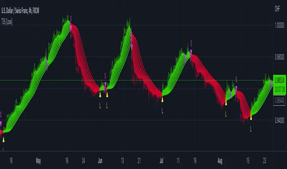
R-squared Adaptive T3 Ribbon Filled Simple [Loxx]R-squared Adaptive T3 Ribbon Filled Simple is a T3 ribbons indicator that uses a special implementation of T3 that is R-squared adaptive.
What is the T3 moving average?
Better Moving Averages Tim Tillson
November 1, 1998
Tim Tillson is a software project manager at Hewlett-Packard, with degrees in Mathematics and Computer Science. He has privately traded options and equities for 15 years.
Introduction
"Digital filtering includes the process of smoothing, predicting, differentiating, integrating, separation of signals, and removal of noise from a signal. Thus many people who do such things are actually using digital filters without realizing that they are; being unacquainted with the theory, they neither understand what they have done nor the possibilities of what they might have done."
This quote from R. W. Hamming applies to the vast majority of indicators in technical analysis . Moving averages, be they simple, weighted, or exponential, are lowpass filters; low frequency components in the signal pass through with little attenuation, while high frequencies are severely reduced.
"Oscillator" type indicators (such as MACD , Momentum, Relative Strength Index ) are another type of digital filter called a differentiator.
Tushar Chande has observed that many popular oscillators are highly correlated, which is sensible because they are trying to measure the rate of change of the underlying time series, i.e., are trying to be the first and second derivatives we all learned about in Calculus.
We use moving averages (lowpass filters) in technical analysis to remove the random noise from a time series, to discern the underlying trend or to determine prices at which we will take action. A perfect moving average would have two attributes:
It would be smooth, not sensitive to random noise in the underlying time series. Another way of saying this is that its derivative would not spuriously alternate between positive and negative values.
It would not lag behind the time series it is computed from. Lag, of course, produces late buy or sell signals that kill profits.
The only way one can compute a perfect moving average is to have knowledge of the future, and if we had that, we would buy one lottery ticket a week rather than trade!
Having said this, we can still improve on the conventional simple, weighted, or exponential moving averages. Here's how:
Two Interesting Moving Averages
We will examine two benchmark moving averages based on Linear Regression analysis.
In both cases, a Linear Regression line of length n is fitted to price data.
I call the first moving average ILRS, which stands for Integral of Linear Regression Slope. One simply integrates the slope of a linear regression line as it is successively fitted in a moving window of length n across the data, with the constant of integration being a simple moving average of the first n points. Put another way, the derivative of ILRS is the linear regression slope. Note that ILRS is not the same as a SMA ( simple moving average ) of length n, which is actually the midpoint of the linear regression line as it moves across the data.
We can measure the lag of moving averages with respect to a linear trend by computing how they behave when the input is a line with unit slope. Both SMA (n) and ILRS(n) have lag of n/2, but ILRS is much smoother than SMA .
Our second benchmark moving average is well known, called EPMA or End Point Moving Average. It is the endpoint of the linear regression line of length n as it is fitted across the data. EPMA hugs the data more closely than a simple or exponential moving average of the same length. The price we pay for this is that it is much noisier (less smooth) than ILRS, and it also has the annoying property that it overshoots the data when linear trends are present.
However, EPMA has a lag of 0 with respect to linear input! This makes sense because a linear regression line will fit linear input perfectly, and the endpoint of the LR line will be on the input line.
These two moving averages frame the tradeoffs that we are facing. On one extreme we have ILRS, which is very smooth and has considerable phase lag. EPMA has 0 phase lag, but is too noisy and overshoots. We would like to construct a better moving average which is as smooth as ILRS, but runs closer to where EPMA lies, without the overshoot.
A easy way to attempt this is to split the difference, i.e. use (ILRS(n)+EPMA(n))/2. This will give us a moving average (call it IE /2) which runs in between the two, has phase lag of n/4 but still inherits considerable noise from EPMA. IE /2 is inspirational, however. Can we build something that is comparable, but smoother? Figure 1 shows ILRS, EPMA, and IE /2.
Filter Techniques
Any thoughtful student of filter theory (or resolute experimenter) will have noticed that you can improve the smoothness of a filter by running it through itself multiple times, at the cost of increasing phase lag.
There is a complementary technique (called twicing by J.W. Tukey) which can be used to improve phase lag. If L stands for the operation of running data through a low pass filter, then twicing can be described by:
L' = L(time series) + L(time series - L(time series))
That is, we add a moving average of the difference between the input and the moving average to the moving average. This is algebraically equivalent to:
2L-L(L)
This is the Double Exponential Moving Average or DEMA , popularized by Patrick Mulloy in TASAC (January/February 1994).
In our taxonomy, DEMA has some phase lag (although it exponentially approaches 0) and is somewhat noisy, comparable to IE /2 indicator.
We will use these two techniques to construct our better moving average, after we explore the first one a little more closely.
Fixing Overshoot
An n-day EMA has smoothing constant alpha=2/(n+1) and a lag of (n-1)/2.
Thus EMA (3) has lag 1, and EMA (11) has lag 5. Figure 2 shows that, if I am willing to incur 5 days of lag, I get a smoother moving average if I run EMA (3) through itself 5 times than if I just take EMA (11) once.
This suggests that if EPMA and DEMA have 0 or low lag, why not run fast versions (eg DEMA (3)) through themselves many times to achieve a smooth result? The problem is that multiple runs though these filters increase their tendency to overshoot the data, giving an unusable result. This is because the amplitude response of DEMA and EPMA is greater than 1 at certain frequencies, giving a gain of much greater than 1 at these frequencies when run though themselves multiple times. Figure 3 shows DEMA (7) and EPMA(7) run through themselves 3 times. DEMA^3 has serious overshoot, and EPMA^3 is terrible.
The solution to the overshoot problem is to recall what we are doing with twicing:
DEMA (n) = EMA (n) + EMA (time series - EMA (n))
The second term is adding, in effect, a smooth version of the derivative to the EMA to achieve DEMA . The derivative term determines how hot the moving average's response to linear trends will be. We need to simply turn down the volume to achieve our basic building block:
EMA (n) + EMA (time series - EMA (n))*.7;
This is algebraically the same as:
EMA (n)*1.7-EMA( EMA (n))*.7;
I have chosen .7 as my volume factor, but the general formula (which I call "Generalized Dema") is:
GD (n,v) = EMA (n)*(1+v)-EMA( EMA (n))*v,
Where v ranges between 0 and 1. When v=0, GD is just an EMA , and when v=1, GD is DEMA . In between, GD is a cooler DEMA . By using a value for v less than 1 (I like .7), we cure the multiple DEMA overshoot problem, at the cost of accepting some additional phase delay. Now we can run GD through itself multiple times to define a new, smoother moving average T3 that does not overshoot the data:
T3(n) = GD ( GD ( GD (n)))
In filter theory parlance, T3 is a six-pole non-linear Kalman filter. Kalman filters are ones which use the error (in this case (time series - EMA (n)) to correct themselves. In Technical Analysis , these are called Adaptive Moving Averages; they track the time series more aggressively when it is making large moves.
What is R-squared Adaptive?
One tool available in forecasting the trendiness of the breakout is the coefficient of determination ( R-squared ), a statistical measurement.
The R-squared indicates linear strength between the security's price (the Y - axis) and time (the X - axis). The R-squared is the percentage of squared error that the linear regression can eliminate if it were used as the predictor instead of the mean value. If the R-squared were 0.99, then the linear regression would eliminate 99% of the error for prediction versus predicting closing prices using a simple moving average .
R-squared is used here to derive a T3 factor used to modify price before passing price through a six-pole non-linear Kalman filter.
Included:
Alerts
Signals
Loxx's Expanded Source Types