Quarterly Theory ICT 01 [TradingFinder] XAMD + Q1-Q4 Sessions🔵 Introduction
The Quarterly Theory ICT indicator is an advanced analytical system based on the concepts of ICT (Inner Circle Trader) and fractal time. It divides time into quarterly periods and accurately determines entry and exit points for trades by using the True Open as the starting point of each cycle. This system is applicable across various time frames including annual, monthly, weekly, daily, and even 90-minute sessions.
Time is divided into four quarters: in the first quarter (Q1), which is dedicated to the Accumulation phase, the market is in a consolidation state, laying the groundwork for a new trend; in the second quarter (Q2), allocated to the Manipulation phase (also known as Judas Swing), sudden price changes and false moves occur, marking the true starting point of a trend change; the third quarter (Q3) is dedicated to the Distribution phase, during which prices are broadly distributed and price volatility peaks; and the fourth quarter (Q4), corresponding to the Continuation/Reversal phase, either continues or reverses the previous trend.
By leveraging smart algorithms and technical analysis, this system identifies optimal price patterns and trading positions through the precise detection of stop-run and liquidity zones.
With the division of time into Q1 through Q4 and by incorporating key terms such as Quarterly Theory ICT, True Open, Accumulation, Manipulation (Judas Swing), Distribution, Continuation/Reversal, ICT, fractal time, smart algorithms, technical analysis, price patterns, trading positions, stop-run, and liquidity, this system enables traders to identify market trends and make informed trading decisions using real data and precise analysis.
♦ Important Note :
This indicator and the "Quarterly Theory ICT" concept have been developed based on material published in primary sources, notably the articles on Daye( traderdaye ) and Joshuuu . All copyright rights are reserved.
🔵 How to Use
The Quarterly Theory ICT strategy is built on dividing time into four distinct periods across various time frames such as annual, monthly, weekly, daily, and even 90-minute sessions. In this approach, time is segmented into four quarters, during which the phases of Accumulation, Manipulation (Judas Swing), Distribution, and Continuation/Reversal appear in a systematic and recurring manner.
The first segment (Q1) functions as the Accumulation phase, where the market consolidates and lays the foundation for future movement; the second segment (Q2) represents the Manipulation phase, during which prices experience sudden initial changes, and with the aid of the True Open concept, the real starting point of the market’s movement is determined; in the third segment (Q3), the Distribution phase takes place, where prices are widely dispersed and price volatility reaches its peak; and finally, the fourth segment (Q4) is recognized as the Continuation/Reversal phase, in which the previous trend either continues or reverses.
This strategy, by harnessing the concepts of fractal time and smart algorithms, enables precise analysis of price patterns across multiple time frames and, through the identification of key points such as stop-run and liquidity zones, assists traders in optimizing their trading positions. Utilizing real market data and dividing time into Q1 through Q4 allows for a comprehensive and multi-level technical analysis in which optimal entry and exit points are identified by comparing prices to the True Open.
Thus, by focusing on keywords like Quarterly Theory ICT, True Open, Accumulation, Manipulation, Distribution, Continuation/Reversal, ICT, fractal time, smart algorithms, technical analysis, price patterns, trading positions, stop-run, and liquidity, the Quarterly Theory ICT strategy acts as a coherent framework for predicting market trends and developing trading strategies.
🔵b]Settings
Cycle Display Mode: Determines whether the cycle is displayed on the chart or on the indicator panel.
Show Cycle: Enables or disables the display of the ranges corresponding to each quarter within the micro cycles (e.g., Q1/1, Q1/2, Q1/3, Q1/4, etc.).
Show Cycle Label: Toggles the display of textual labels for identifying the micro cycle phases (for example, Q1/1 or Q2/2).
Table Display Mode: Enables or disables the ability to display cycle information in a tabular format.
Show Table: Determines whether the table—which summarizes the phases (Q1 to Q4)—is displayed.
Show More Info: Adds additional details to the table, such as the name of the phase (Accumulation, Manipulation, Distribution, or Continuation/Reversal) or further specifics about each cycle.
🔵 Conclusion
Quarterly Theory ICT provides a fractal and recurring approach to analyzing price behavior by dividing time into four quarters (Q1, Q2, Q3, and Q4) and defining the True Open at the beginning of the second phase.
The Accumulation, Manipulation (Judas Swing), Distribution, and Continuation/Reversal phases repeat in each cycle, allowing traders to identify price patterns with greater precision across annual, monthly, weekly, daily, and even micro-level time frames.
Focusing on the True Open as the primary reference point enables faster recognition of potential trend changes and facilitates optimal management of trading positions. In summary, this strategy, based on ICT principles and fractal time concepts, offers a powerful framework for predicting future market movements, identifying optimal entry and exit points, and managing risk in various trading conditions.
Cari dalam skrip untuk "Fractal"

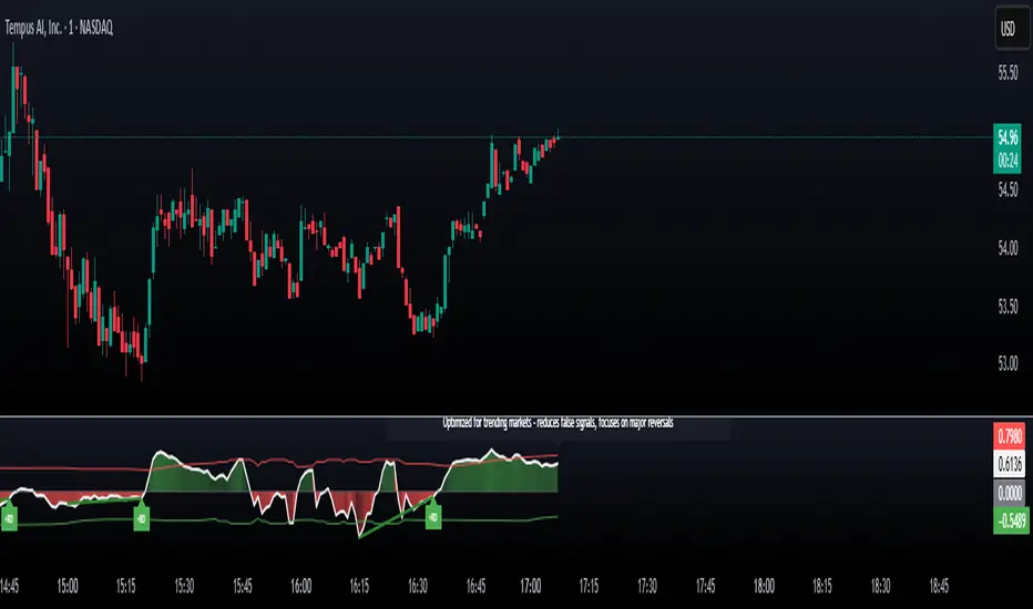
Market Participation Index [PhenLabs]📊 Market Participation Index
Version: PineScript™ v6
📌 Description
Market Participation Index is a well-evolved statistical oscillator that constantly learns to develop by adapting to changing market behavior through the intricate mathematical modeling process. MPI combines different statistical approaches and Bayes’ probability theory of analysis to provide extensive insight into market participation and building momentum. MPI combines diverse statistical thinking principles of physics and information and marries them for subtle changes to occur in markets, levels to become influential as important price targets, and pattern divergences to unveil before it is visible by analytical methods in an old-fashioned methodology.
🚀 Points of Innovation:
Automatic market condition detection system with intelligent preset selection
Multi-statistical approach combining classical and advanced metrics
Fractal-based divergence system with quality scoring
Adaptive threshold calculation using statistical properties of current market
🚨 Important🚨
The ‘Auto’ mode intelligently selects the optimal preset based on real-time market conditions, if the visualization does not appear to the best of your liking then select the option in parenthesis next to the auto mode on the label in the oscillator in the settings panel.
🔧 Core Components
Statistical Foundation: Multiple statistical measures combined with weighted approach
Market Condition Analysis: Real-time detection of market states (trending, ranging, volatile)
Change Point Detection: Bayesian analysis for finding significant market structure shifts
Divergence System: Fractal-based pattern detection with quality assessment
Adaptive Visualization: Dynamic color schemes with context-appropriate settings
🔥 Key Features
The indicator provides comprehensive market analysis through:
Multi-statistical Oscillator: Combines Z-score, MAD, and fractal dimensions
Advanced Statistical Components: Includes skewness, kurtosis, and entropy analysis
Auto-preset System: Automatically selects optimal settings for current conditions
Fractal Divergence Analysis: Detects and grades quality of divergence patterns
Adaptive Thresholds: Dynamically adjusts overbought/oversold levels
🎨 Visualization
Color-coded Oscillator: Gradient-filled oscillator line showing intensity
Divergence Markings: Clear visualization of bullish and bearish divergences
Threshold Lines: Dynamic or fixed overbought/oversold levels
Preset Information: On-chart display of current market conditions
Multiple Color Schemes: Modern, Classic, Monochrome, and Neon themes
Classic
Modern
Monochrome
Neon
📖 Usage Guidelines
The indicator offers several customization options:
Market Condition Settings:
Preset Mode: Choose between Auto-detection or specific market condition presets
Color Theme: Select visual theme matching your chart style
Divergence Labels: Choose whether or not you’d like to see the divergence
✅ Best Use Cases:
Identify potential market reversals through statistical divergences
Detect changes in market structure before price confirmation
Filter trades based on current market condition (trending vs. ranging)
Find optimal entry and exit points using adaptive thresholds
Monitor shifts in market participation and momentum
⚠️ Limitations
Requires sufficient historical data for accurate statistical analysis
Auto-detection may lag during rapid market condition changes
Advanced statistical calculations have higher computational requirements
Manual preset selection may be required in certain transitional markets
💡 What Makes This Unique
Statistical Depth: Goes beyond traditional indicators with advanced statistical measures
Adaptive Intelligence: Automatically adjusts to current market conditions
Bayesian Analysis: Identifies statistically significant change points in market structure
Multi-factor Approach: Combines multiple statistical dimensions for confirmation
Fractal Divergence System: More robust than traditional divergence detection methods
🔬 How It Works
The indicator processes market data through four main components:
Market Condition Analysis:
Evaluates trend strength, volatility, and price patterns
Automatically selects optimal preset parameters
Adapts sensitivity based on current conditions
Statistical Oscillator:
Combines multiple statistical measures with weights
Normalizes values to consistent scale
Applies adaptive smoothing
Advanced Statistical Analysis:
Calculates higher-order statistical moments
Applies information-theoretic measures
Detects distribution anomalies
Divergence Detection:
Uses fractal theory to identify pivot points
Detects and scores divergence quality
Filters signals based on current market phase
💡 Note:
The Market Participation Index performs optimally when used across multiple timeframes for confirmation. Its statistical foundation makes it particularly valuable during market transitions and periods of changing volatility, where traditional indicators often fail to provide clear signals.
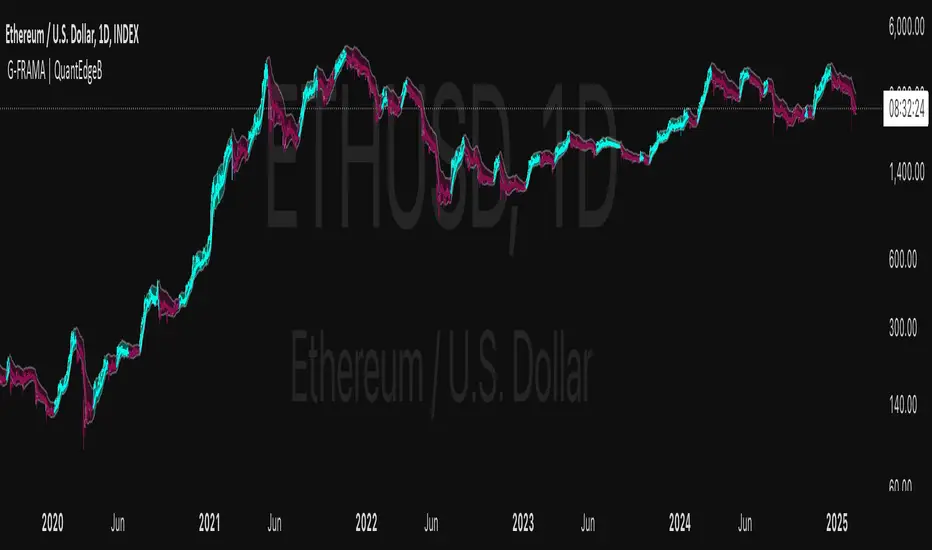
G-FRAMA | QuantEdgeBIntroducing G-FRAMA by QuantEdgeB
Overview
The Gaussian FRAMA (G-FRAMA) is an adaptive trend-following indicator that leverages the power of Fractal Adaptive Moving Averages (FRAMA), enhanced with a Gaussian filter for noise reduction and an ATR-based dynamic band for trade signal confirmation. This combination results in a highly responsive moving average that adapts to market volatility while filtering out insignificant price movements.
_____
1. Key Features
- 📈 Gaussian Smoothing – Utilizes a Gaussian filter to refine price input, reducing short-term noise while maintaining responsiveness.
- 📊 Fractal Adaptive Moving Average (FRAMA) – A self-adjusting moving average that adapts its sensitivity to market trends.
- 📉 ATR-Based Volatility Bands – Dynamic upper and lower bands based on the Average True Range (ATR), improving signal reliability.
- ⚡ Adaptive Trend Signals – Automatically detects shifts in market structure by evaluating price in relation to FRAMA and its ATR bands.
_____
2. How It Works
- Gaussian Filtering
The Gaussian function preprocesses the price data, giving more weight to recent values and smoothing fluctuations. This reduces whipsaws and allows the FRAMA calculation to focus on meaningful trend developments.
- Fractal Adaptive Moving Average (FRAMA)
Unlike traditional moving averages, FRAMA uses fractal dimension calculations to adjust its smoothing factor dynamically. In trending markets, it reacts faster, while in sideways conditions, it reduces sensitivity, filtering out noise.
- ATR-Based Volatility Bands
ATR is applied to determine upper and lower thresholds around FRAMA:
- 🔹 Long Condition: Price closes above FRAMA + ATR*Multiplier
- 🔻 Short Condition: Price closes below FRAMA - ATR
This setup ensures entries are volatility-adjusted, preventing premature exits or false signals in choppy conditions.
_____
3. Use Cases
✔ Adaptive Trend Trading – Automatically adjusts to different market conditions, making it ideal for both short-term and long-term traders.
✔ Noise-Filtered Entries – Gaussian smoothing prevents false breakouts, allowing for cleaner entries.
✔ Breakout & Volatility Strategies – The ATR bands confirm valid price movements, reducing false signals.
✔ Smooth but Aggressive Shorts – While the indicator is smooth in overall trend detection, it reacts aggressively to downside moves, making it well-suited for traders focusing on short opportunities.
_____
4. Customization Options
- Gaussian Filter Settings – Adjust length & sigma to fine-tune the smoothness of the input price. (Default: Gaussian length = 4, Gaussian sigma = 2.0, Gaussian source = close)
- FRAMA Length & Limits – Modify how quickly FRAMA reacts to price changes.(Default: Base FRAMA = 20, Upper FRAMA Limit = 8, Lower FRAMA Limit = 40)
- ATR Multiplier – Control how wide the volatility bands are for long/short entries.(Default: ATR Length = 14, ATR Multiplier = 1.9)
- Color Themes – Multiple visual styles to match different trading environments.
_____
Conclusion
The G-FRAMA is an intelligent trend-following tool that combines the adaptability of FRAMA with the precision of Gaussian filtering and volatility-based confirmation. It is versatile across different timeframes and asset classes, offering traders an edge in trend detection and trade execution.
____
🔹 Disclaimer: Past performance is not indicative of future results. No trading strategy can guarantee success in financial markets.
🔹 Strategic Advice: Always backtest, optimize, and align parameters with your trading objectives and risk tolerance before live trading.
ZenAlgo - Aggregated DeltaZenAlgo - Aggregated Delta is an advanced market analysis tool designed to provide traders with a holistic view of market sentiment by leveraging multi-exchange volume aggregation, cumulative delta analysis, and divergence detection. Unlike traditional indicators that rely on a single data source, this tool aggregates order flow data from multiple exchanges, reducing the impact of exchange-specific anomalies and liquidity disparities.
This indicator is ideal for traders looking to enhance their understanding of market dynamics, trend confirmations, and order flow patterns. By intelligently combining multiple analytical components, it eliminates the need for manually interpreting separate indicators and offers traders a streamlined approach to market analysis.
This indicator was inspired by aggregated volume analysis techniques. Independently developed with a focus on cumulative delta and divergence detection.
Key Features & Their Interaction
Multi-Exchange Volume Aggregation: Aggregates buy and sell volumes from up to nine major exchanges, including Binance, Bybit, Coinbase, and Kraken. Unlike traditional single-source indicators, this ensures a robust, diversified measure of market sentiment and smooths out exchange-specific volume fluctuations.
Cumulative Delta Analysis: Tracks the net difference between buy and sell volumes across all aggregated exchanges, helping traders identify true buying/selling pressure rather than misleading short-term volume spikes.
Advanced Divergence Detection: Unlike basic divergence indicators, this tool detects divergences not only between price and cumulative delta but also across multiple analytical layers, including moving averages and temperature zones, offering deeper confirmation signals.
Dynamic Market Temperature Zones: Unlike fixed overbought/oversold indicators, this feature applies adaptive standard deviation-based filtering to classify market conditions dynamically as "Extreme Hot," "Hot," "Neutral," "Cold," and "Extreme Cold."
Intelligent Market State Classification: Determines whether the market is in a Full Bull, Bearish, or Neutral state by analyzing multi-exchange volume flow, cumulative delta positioning, and market-wide liquidity trends.
Real-Time Alerts & Adaptive Visualization: Provides fully configurable real-time alerts for trend shifts, divergences, and market conditions, allowing traders to act immediately on high-confidence signals.
What Makes ZenAlgo - Aggregated Delta Unique?
Unlike free or open-source alternatives, ZenAlgo - Aggregated Delta applies a multi-layered data processing approach to smooth inconsistencies and improve signal reliability. Instead of using raw exchange feeds, the system incorporates adaptive volume aggregation and standard deviation-based market classification to ensure accuracy and reduce noise. These enhancements lead to more precise trend signals and a clearer representation of market sentiment.
Multi-Exchange Order Flow Validation: Unlike single-source indicators that rely on individual exchange feeds, this tool ensures cross-market consistency by aggregating volume data dynamically.
Fractal-Based Divergence Detection: Detects divergences using fractal logic rather than contextual volume trends, reducing false-positive divergence signals while maintaining accuracy.
Automated Sentiment Analysis: Classifies market sentiment into structured phases (Full Bull, Bearish, etc.), reducing the manual effort needed to interpret order flow trends.
How It Works (Technical Breakdown)
Multi-Exchange Volume Aggregation: The system fetches and validates buy/sell volume data from multiple exchanges, applying volume aggregation techniques to smooth out inconsistencies. It ensures that data from low-liquidity exchanges does not disproportionately influence the analysis.
Cumulative Delta Computation: Cumulative delta is computed as the net difference between buy and sell volumes over a given period. By summing up these values across multiple exchanges, traders can identify real accumulation or distribution zones, reducing false signals from isolated exchange anomalies.
Divergence Detection Methodology: The tool uses a fractal-based logic approach to detect high-confidence divergences across price, volume, and delta trends. This allows for a more structured detection process compared to simple peak/trough analysis, reducing noise in the signals.
Temperature Zones Filtering: Market conditions are dynamically classified using a rolling standard deviation model, ensuring that hot/cold states adjust automatically based on recent volatility levels. This means that instead of using arbitrary fixed thresholds, the tool adapts based on historical data behavior.
Market Sentiment State Calculation: The tool evaluates liquidity conditions, volume trends, and cumulative delta flow, categorizing the market into predefined states (Bullish, Bearish, Neutral). This helps traders assess the broader context of price movements rather than reacting to isolated signals.
Real-Time Adaptive Alerts: The system provides fully configurable alerts that notify traders about key trend shifts, high-confidence divergences, and changes in market conditions as they occur. This ensures that traders can make timely and well-informed decisions.
Why This Approach Works
By aggregating data from multiple exchanges, it reduces the impact of exchange-specific liquidity disparities and anomalies, leading to a more holistic view of order flow.
The cumulative delta analysis ensures that price movements are validated by actual buying/selling pressure, filtering out misleading short-term spikes.
Dynamic market classification adapts to current conditions rather than using outdated fixed thresholds, making it more relevant in different market regimes.
Fractal-based divergence detection avoids common pitfalls of traditional divergence analysis, reducing false signals while maintaining accuracy.
Combining real-time adaptive alerts with well-structured classification improves traders’ ability to respond to market shifts efficiently.
Practical Use Cases
Identifying High-Probability Trend Reversals: If cumulative delta shows bullish divergence while the market is in an Extreme Cold zone, it signals a strong potential for reversal.
Confirming Trend Continuation: When bullish moving average crossovers align with a rising cumulative delta, traders can enter positions with higher confidence.
Detecting Exhaustion in Market Moves: If price enters an "Extreme Hot" zone but cumulative delta starts declining, this suggests trend exhaustion and a possible reversal.
Filtering False Breakouts: If price breaks a resistance level but aggregated buy volume fails to increase, this invalidates the breakout, helping traders avoid bad trades.
Cross-Exchange Sentiment Confirmation: If cumulative delta on aggregated exchanges contradicts price action on an individual exchange, traders can identify localized exchange-based distortions.
Customization & Settings Overview
Exchange Selection: Traders can fine-tune exchange sources for aggregation, allowing for custom market-specific insights.
Adaptive Divergence Settings: Configure detection thresholds, lookback periods, and divergence filtering options to reduce noise and focus on high-confidence signals.
Moving Average Adjustments: Select custom MA types, lengths, and visualization preferences to match different trading styles.
Market Temperature Thresholds: Adjust hot/cold sensitivity to align with preferred risk levels and volatility expectations.
Configurable Alerts & Theme Customization: Full control over notification triggers, color themes, and label formatting to enhance user experience.
Important Considerations
Market Context Dependency: This tool provides order flow analysis, which should be used in conjunction with broader market context and risk management.
Data Source Variability: While multi-exchange aggregation improves reliability, some exchanges may report inaccurate or delayed data.
Extreme Volatility Handling: Large price swings can temporarily distort delta readings, so traders should always validate with additional context.
Liquidity Limitations: In low-liquidity conditions, order flow signals may be less reliable due to fragmented market participation.

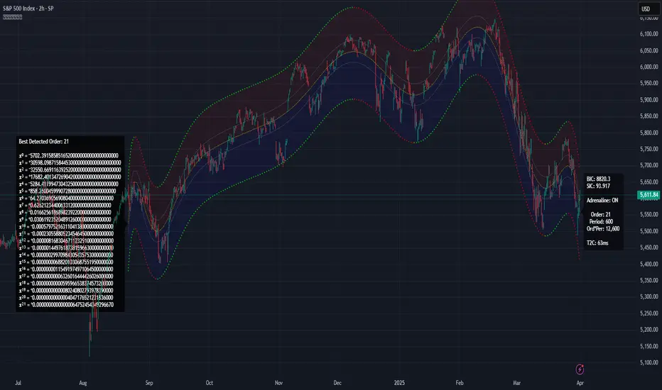
[Excalibur] Advanced Polynomial Regression Trend ChannelIt's been a long time coming... Regression channel enthusiasts, it's 'ultimately' here! Welcome to my Apophis page. But first, let me explain the origins of its attributed name blending both descriptive & engaging content with concise & technical topics...
EGYPTIAN ROOTED TALES:
Apophis (Greek) or Apep (Egyptian) was known by many cultures to be a mighty Egyptian archetype of chaos, darkness, and destruction. In ancient Egyptian mythology, Apophis was often depicted in the form of a fearsome menacing serpent, in those days, with an insatiable appetite for relentless malevolence. This dreaded entity was considered a formidable enemy and was also believed to appear as a giant serpent arising from the underworld.
Forever engaging in eternal battle, according to lore, Apophis' adversarial attributes represented the forces of disorder and anarchy clashing with the forces of order and harmony. This serpent's wickedly described figure was significantly symbolic of the disruptive, treacherous powers that Apophis embodied, those which threatened to plunge the perceivable archaic world into darkness. To the ancients, the legendary cyclical struggles against Apophis served as allegory reflecting on the macrocosm of the larger conflict between good and evil disparities that shaped early ancient civilization, much like the tree serpent.
One of Apophis’ mythological roots was immortally depicted on tomb stone. On one particular hieroglyphic wall tableau, in the second chamber of Inherkau’s tomb at Deir el-Medina, within the Theban Necropolis, portrays a mural of a serpent (Apep) under an edible fruit tree being slain in defeat. The species of snake depicted on various locations of tomb walls appears to me to bear a striking resemblance to the big eyed Echis pyramidum (Egyptian saw-scaled viper) native to regions of North Africa and the Middle East. It's a species of viper notoriously contributing to the most snake bite fatalities in the world still to this day; talk about a true harbinger of chaos incarnate. You do NOT want to cross paths with this asp in the dark of night, ever! Nor the other species of Echis found around Echid trees in the garden.
As we all know, fabled archaic storytelling can be misconstruing. Yet, these archaic serpent narratives still have echoes of significant notions and wisdom to learn from, especially in a modern technological society still rife with miscalculating deep snakes slithering about with intent to specifically plot disorder on national scales, and then profitably capitalize on it. Many deep black snakes are hiding in plain sight and under rocks. They do indeed speak and spell with forked tongues and malfeasance to the masses. I have great news. Tools now exist in the realms of AI combined with fractal programming circles to uncover these venomous viper mesh networks and investigatively monitor their subversive activities, so their days are surely numbered for... GAME OVER. Prepare to meet the doom you vain vipers have sought!
The arrival of the great and powerful international storm of the century has come, clothed in vindication. It's the only just way for the globe to clean house and move forward economically into the evolving herafter unobstructed by rampant evils and corruption. The foundations of future architectures are being established, and these nefarious obstacles MUST NOT hinder that path ahead.
With my former days of serpent wrangling being behind me, I now explore avenues of history, philosophy, programming, and mathematics, weaving them all into my daily routine. Now is the time to make some mathematical history unfold and get to the good and spicy stuff that you as the reader seek...
CALCULATING ON CHAOS:
Perhaps frightful characteristics of serpents (their maneuverability to adapt to any swervy situation) could be harnessed and channeled into a powerful tool for navigating the treacherous waters of data chaos. What if taming a monstrous beast of mayhem was not only possible, but fully achievable? Well, I think I have improved upon an approach to better tackle fractal chaos handling and observation within a modest PSv6 float environment without doubles. Finally, I've successfully turned my pet anaconda, Apophis, into a docile form of mathematical charting resilience beyond anything I have ever visually witnessed before. This novel work clearly deprecates ALL of my prior regression works by performing everything those delivered AND more, but it doesn't necessarily eliminate them into extinction.
INTRODUCTION:
Allow me to introduce Apophis! What you see showcased above is also referred to as 'Advanced Polynomial Regression Trend Channel' (APRTC) for technical minds. I would describe it as an avant-garde trend channel obtaining accurate polynomial approximations on market data with Pine v6.0. APRTC is a fractal following demystifier that I can only describe as being a signal trajectory tracking stalker manifesting as a data devouring demon. My full-fledged 'Excalibur' version of poly-regression swiftly captures undulating patterns present in market data with ease and at warp speed faster than you can blink. Now unchained, this is my rendering of polynomial wrath employing the "Immense Power of Pine".
By pushing techniques of regression to extremes, I am able to trace the serpentine trajectory of chaos up to a 50th order with 100s or 1000s of samples via "advanced polynomial regression" (APR), aka Apophis. This uniquely reactive trend channel method is designed to enhance the way we engage with the complex challenge of observably interpreting chaotic price behavior. While this is the end of the road for my revolutionary trend channel technology, that doesn't imply that future polynomial regression upgrades won't/might occur... There are a number of other supplementary concepts I have in my mind that could potentially prove useful eventually, who knows. However, for the moment, I feel it's wisest to monitor how accommodating APRTC is towards servers for the present time.
HISTORICAL ENDEAVORS:
Having wrangled countless wild serpents in my youth by the handfuls, tackling this was one multi-headed regression challenge temptation I couldn't resist. Besides, serpents in reality are more than often scared of us in the wild, so I assumed this shouldn't be too terribly hard. Wrong! It's been a complex struggle indeed. APRTC gave me many stinging bites for a LONG time. I had unknowingly opened Pandora's box of polynomials unprepared for what was to follow.
Long have I wrestled with Apophis throughout many nights for years with adversity, at last having arrived at a current grand solution and ultimately emerging victorious. Now, does the significance of the entitled name Apophis become more apparent at this point of reading? What you can now witness above is a very powerful blend of precision combined with maneuverability, concluding my dreamy expectations of a maximal experience with polynomial regression in TV charts. With all of my wizardry components finally assembled, Apophis genuinely is the most phenomenal indicator I ever devised in my life... as of yet.
How was this accomplished? By unlocking a deep understanding of the mathematical principles that govern regression, combined with an arsenal of mathemagical trickeries through sheer determination. I also spent an incredible amount of time flexing the unbendable 64bit float numerics to obtain a feasible order/degree of up to 50 polynomials or up to 4000 bars of regression (never simultaneously) on a labyrinth of samples. Lastly, what was needed was a pinch of mathematical pixie dust with a pleasant dose of Pine upgrades (lots of line re-drawings) that millions of other members can also utilize. Thank you so much, Pine developers, for once again turning meager proposed visions into materialized reality by leveraging the "Power of Pine" for the many!
DESCRIBING POLYNOMIAL REGRESSION:
APRTC is a visual guide for navigating noisy markets, providing both trajectory and structure through the power of mathematical modeling. Polynomial regression, especially at higher orders, exhibits obvious sidewinder/serpentine like characteristics. Even the channel extremities, on swift one second charts, resemble scales in motion with a pair of dashed exterior lines. This poly version presently yields the best quality of fit, providing an extreme "visual analysis" of your price action in high noise environments. The greater the order of the polynomial, the more pronounced the meandering regression characteristics become, as the algorithm strives to visually capture the fundamental fractal patterns most effectively.
Polynomial Regression in Action:
The medial line displays the core polynomial regression approximation in similarity to spinal backbones of serpents when following the movements of market data. Encasing the central structure, the channel's skin consists of enveloping lines having upper and lower extremes. To further enhance visualization, background fill colors distinguish the breadth between positive and negative territories of potential movement.
Additional internal dotted variability lines are available with multiple customizable settings to adjust dynamic dispersion, color, etc. One other exciting feature I added is the the ability to see the polynomial values with up to 50 (adjustable) decimal places if available. Witnessing Xⁿ values tapering near to 0.0 may indicate overfitting. Linear regression is available at order=1 and quadratic regression is invoked using order=2.
Information Criterion:
A toggleable label provides a multitude of information such as Bayesian Information Criterion (BIC), order, period, etc. BIC serves as an polynomial regression fit metric, with lesser values indicating a better balance between polynomial order adjustments, reflecting a more accurate fit in relation to the channel's girth. One downside of BIC values is their often large numerical values, making visual comparisons challenging, and then also their rare occurrence as negative values.
Furthermore, I formulated my own "EXPERIMENTAL" Simpler Information Criterion (SIC) fit metric, which seems to offer better visual interpretability when adjusting order settings on a selected regression period, especially on minuscule price numerics. Positive valued SIC numerics with lesser digits also reflect a preferred better fit during order adjustment, same as applying BIC principles of the minimum having a superior calulation tendency. I'll let members be the judge of deciding whether my SIC is actually a superior information criterion compared to BIC.
TECHNICAL INTERPRETATION and APPLICATION:
The Apophis indicator utilizes high-order polynomial regression, up to a maximum 50th order ability to deliver a nuanced, visual representation of complex market dynamics. I would caution against using upwards toward a 50th order, because opting for a 50th order polynomial is categorically speaking "wildly unsane" in real-world practice. As the polynomial degree increases from lesser orders, the regression line exhibits more pronounced curvature and undulations.
Visually analyzing the regression curve can provide insights into prevailing trends, as well as volatility regimes. For example, a gently sloping line may signal a steady directional trend, while a tightly curled oscillating curve may indicate heightened volatility and range-bound trading. Settings are rather straight forward, and comparable to my former "Quadratic Regression Trend Channel" efforts, although one torturous feature from QRTC is omitted due too computational complexity concerns.
Notice: Trial invite only access will not be granted for this indicator. Those who are familiar with recognizing what APRTC is, you will either want it or not, to add to your arsenal of trading approaches.
When available time provides itself, I will consider your inquiries, thoughts, and concepts presented below in the comments section, should you have any questions or comments regarding this indicator. When my indicators achieve more prevalent use by TV members , I may implement more ideas when they present themselves as worthy additions. Have a profitable future everyone!
RISK DISCLAIMER:
My scripts and indicators are specifically intended for informational and educational use only. This script uses historical data points to perform calculations to derive real-time calculations. They do not infer, indicate, or guarantee future results or performance.
By utilizing this script/indicator or any portion of it, you agree to accept 100% responsibly and liability for your investment or financial decisions, and I will not be held liable for your subjective analytic interpretations incurring sustained monetary losses. The opinions and information visual or otherwise provided by this script/indicator is not investment advice, nor does it constitute recommendation.
Aso Line v2This indicator generates buy and sell signals by analyzing volume and horizontal lines. Red and green zones are displayed on the chart.
・Red zone: indicates a short (sell) signal. When the price reaches this zone, consider a short position.
・Green zone: indicates a long (buy) signal. When the price reaches this zone, consider a long position.
This indicator uses a proprietary algorithm to analyze volume and horizontal lines to identify the best zones for trading. Specifically, we will explain and .
In addition, configuration options for using this indicator effectively will be explained. For example, there are parameters to adjust the width of the zone, the volume calculation period, and the type of horizontal line used. By adjusting these parameters, you can adapt to different market conditions and trading styles.
- The way this indicator works is to look for fractal highs or fractal lows on volume above a moving average of volume. This moving average can be changed in the settings for each time frame.
- Fractal highs are identified by three consecutive highs followed by two consecutive lows, and vice versa for fractal lows.
- A zone is created from the fractal high/low and the closing candlestick price for the selected time frame. The larger the zone, the more important it is.
- You can disable zones, change zones to show only lines, or change the color, transparency, and thickness of lines in all zones.

BOS TRADER [v 1.0] [Influxum]The name of the tool, BOS Trader, comes from the abbreviation BOS, which stands for Break Of Structure. In simple terms, this tool identifies situations where a change in market structure occurs after liquidity has been grabbed. Following the structural change, it looks for a point where the balance between buyers and sellers will be tested, potentially continuing the price movement in the direction of the structural break.
The goal of this tool is to identify areas where a trader can look for potential entry opportunities based on their entry rules and filters. In our own research, we found that while this tool is not a standalone strategy, it provides a statistical advantage that stems from the nature of the market itself. If you expect the market to reverse at a certain price level against a short-term, medium-term, or long-term trend, that reversal must logically begin with a change in structure – i.e., its break. BOS Trader then highlights the zone where you can expect a strong reaction from traders speculating on the continuation of price in the direction of the break.
Another important piece of the puzzle is the concept of liquidity. Liquidity grabs are generally considered by traders to be events that can trigger market direction changes. That's why BOS Trader is complemented with multiple ways to identify liquidity in the market from a Price Action perspective. We have explored the liquidity concept in depth in our other tools – the Liquidity Tool and Liquidity Strategy Tester – so we won’t go into too much detail on liquidity settings here.
🟪 Pivots
Liquidity can be found beyond pivot extremes – the highest candles in a series of candles. The pivot liquidity setting specifies how many candles must be before and after the pivot candle with a lower high for a pivot high or a higher low for a pivot low. A pivot high is the local highest point of the last 31 candles (15 before the pivot candle, the pivot candle itself, and 15 after). Another option is to set the time period in which the pivot extreme must occur. For example, you can differentiate between pivot highs of the Asian or London session.
🟪 % Percent Change
This setting is based on the well-known Zig Zag indicator and confirms swing highs or swing lows when there is a certain percentage change in price. This helps filter out noise that can occur when the market consolidates and randomly creates pivot highs or lows that aren’t significant.
🟪 Session High/Low
Many popular strategies are based on liquidity defined as the price range of a specific trading session. This doesn't have to be London, Asia, or New York sessions, but could be, for instance, the first hour of the New York session, and so on.
🟪 Day High/Low, Week High/Low, Month High/Low
As the name suggests, liquidity is often defined by the high/low of the previous day, week, or month. These price levels are watched by many market participants, and it's reasonable to expect reactions at these levels. That’s why we included this option in the BOS tool.
Tip for Traders
To avoid common issues with setting the correct session time, we have added the BG option to the tool – the ability to display a background for the configured trading session. This makes it easy to verify that your trading session is set correctly in relation to your time zone.
Delete grabbed liquidity
If a liquidity level is breached by price, it becomes invalid. For those who prefer to keep their charts clean and uncluttered, there is an option to delete grabbed liquidity. This way, only untraded, valid liquidity lines will be visible on the chart.
Bars after liquidity grab
A liquidity grab should be a significant event that triggers a reaction from market participants. To ensure this is a real response to liquidity rather than random market behavior, we added a time test to the BOS tool. A structural break must occur within a specified time after the liquidity grab. You can define this time in the tool as the number of bars after which the structural break is still considered valid following the liquidity grab.
🟪 AOI (Area of Interest) Settings
Initially, it's important to note that there are two main options for setting the behavior of the AOI. The first option is to fix its duration by the number of bars – Duration, and the second is to keep the AOI valid until it is traded through – Extended.
Duration
Since we expect a quick reaction to the liquidity grab, we also expect a fast pullback to the AOI and a swift response of traders. Our research has shown that the strongest reactions typically occur within a maximum of 15 bars from the formation of the AOI (fractally across timeframes). Therefore, this value is set as the default. However, we recommend considering not just the speed of the reaction but also its intensity. After the set number of bars, the AOI stops extending further.
Extended
We have noticed that price has a tendency to return to the AOI even after a longer period and react again. For this reason, we included the option in the BOS tool to extend the AOI into the future, with the ability to freely adjust the Max AOI Length.
🟪 AOI Size Mode
There are two options for setting the size of the AOI. Either it can be calculated as a percentage of the swing size (% of swing) in which the structural break occurred (the default setting is 30%), or you can set a different concept for the AOI size. For example, the well-known Optimal Trade Entry model. Custom values can be set in the FIBO Levels option, where you can define either preferred Fibonacci values or values based on your own criteria.
🟪 Trading Session (signals + alerts + visibility)
The main goal of our tools is to make it easier for traders to identify patterns and opportunities in the market and allow them to be alerted to their occurrence. The time for AOI plotting after a liquidity grab is combined into a single Trading Session function. This controls both the AOI plotting and when the tool will send alerts. All of this is aimed at helping traders avoid spending the entire day in front of their monitors, waiting for trading opportunities. Here, too, you can use the BG feature to plot a background on the chart showing the current session.
🟪 Trading within session range
We found that some traders have difficulty navigating the many AOIs plotted during times when the market consolidates and creates numerous false breakouts. Therefore, we included an option in the BOS tool to track only structural changes at the price extremes of the current day and trading session. The tool will not plot structural changes for internal liquidity grabs (within the session range), but only for external liquidity grabs (highest highs and lowest lows of the session or liquidity from previous days).
Visuals
The BOS tool is, of course, supplemented with the option to customize the appearance of all its components according to your preferences.

Market DirectionThe "Market Direction" indicator combines four advanced sub-indicators to provide a comprehensive and multi-dimensional analysis of market trends, momentum, and potential reversals. This innovative approach leverages different aspects of price action, volume, and market sentiment, offering traders an in-depth view of market conditions.
1. Fractal Indicator: Multi-Scale Price Action Analysis
The Fractal Indicator identifies significant highs and lows over six different pivot lengths, offering a nuanced view of price action across multiple timeframes. By comparing distances from current closing prices to these key fractal points, the indicator determines potential trend reversals and market direction. This approach enables traders to adapt their strategies to various market conditions, capturing both short-term fluctuations and long-term trends.
2. Volume MACD Indicator: Enhanced Market Momentum
The Volume MACD Indicator goes beyond traditional MACD analysis by incorporating volume-weighted movement and the structural attributes of candlesticks (such as body length and wicks). This hybrid model offers a more comprehensive understanding of market momentum by integrating both price action and trading volume. The use of Smoothed Moving Averages (SMMA) reduces noise and ensures more stable signals, helping traders focus on sustainable trends and longer-term investment opportunities.
3. Cumulative Volume Momentum Indicator: Volume Dynamics Insight
The Cumulative Volume Momentum Indicator evaluates the momentum of cumulative buying and selling volumes, offering a clear picture of market strength and potential reversals. By comparing the relationship between open, close, high, and low prices, and applying a MACD approach to these volume dynamics, this indicator helps traders identify momentum shifts that often precede price movements. The visualization through histograms adds clarity to bullish and bearish volume momentum, enhancing decision-making in volatile markets.
4. POC-Price Momentum Indicator: Market Depth and Sentiment
The POC-Price Momentum Indicator assesses the difference between the Point of Control (POC) and closing prices, providing insights into underlying market sentiment. Positive differences indicate a buildup of upward momentum, while negative differences suggest a bearish tilt. By calculating moving averages of these differences, the indicator highlights the strength and sustainability of ongoing trends, helping traders align their strategies with the broader market direction.
Unified Rating for Confirming Market Direction
The "Market Direction" indicator consolidates the outputs of these four sub-indicators into a single, aggregated sentiment score. This score helps traders confirm the prevailing market trend by weighing the combined insights from fractal analysis, volume momentum, price action, and POC dynamics. A positive score suggests a bullish market, while a negative score indicates bearish conditions.

Six PillarsGeneral Overview
The "Six Pillars" indicator is a comprehensive trading tool that combines six different technical analysis methods to provide a holistic view of market conditions.
These six pillars are:
Trend
Momentum
Directional Movement (DM)
Stochastic
Fractal
On-Balance Volume (OBV)
The indicator calculates the state of each pillar and presents them in an easy-to-read table format. It also compares the current timeframe with a user-defined comparison timeframe to offer a multi-timeframe analysis.
A key feature of this indicator is the Confluence Strength meter. This unique metric quantifies the overall agreement between the six pillars across both timeframes, providing a score out of 100. A higher score indicates stronger agreement among the pillars, suggesting a more reliable trading signal.
I also included a visual cue in the form of candle coloring. When all six pillars agree on a bullish or bearish direction, the candle is colored green or red, respectively. This feature allows traders to quickly identify potential high-probability trade setups.
The Six Pillars indicator is designed to work across multiple timeframes, offering a comparison between the current timeframe and a user-defined comparison timeframe. This multi-timeframe analysis provides traders with a more comprehensive understanding of market dynamics.
Origin and Inspiration
The Six Pillars indicator was inspired by the work of Dr. Barry Burns, author of "Trend Trading for Dummies" and his concept of "5 energies." (Trend, Momentum, Cycle, Support/Resistance, Scale) I was intrigued by Dr. Burns' approach to analyzing market dynamics and decided to put my own twist upon his ideas.
Comparing the Six Pillars to Dr. Burns' 5 energies, you'll notice I kept Trend and Momentum, but I swapped out Cycle, Support/Resistance, and Scale for Directional Movement, Stochastic, Fractal, and On-Balance Volume. These changes give you a more dynamic view of market strength, potential reversals, and volume confirmation all in one package.
What Makes This Indicator Unique
The standout feature of the Six Pillars indicator is its Confluence Strength meter. This feature calculates the overall agreement between the six pillars, providing traders with a clear, numerical representation of signal strength.
The strength is calculated by considering the state of each pillar in both the current and comparison timeframes, resulting in a score out of 100.
Here's how it calculates the strength:
It considers the state of each pillar in both the current timeframe and the comparison timeframe.
For each pillar, the absolute value of its state is taken. This means that both strongly bullish (2) and strongly bearish (-2) states contribute equally to the strength.
The absolute values for all six pillars are summed up for both timeframes, resulting in two sums: current_sum and alternate_sum.
These sums are then added together to get a total_sum.
The total_sum is divided by 24 (the maximum possible sum if all pillars were at their strongest states in both timeframes) and multiplied by 100 to get a percentage.
The result is rounded to the nearest integer and capped at a minimum of 1.
This calculation method ensures that the Confluence Strength meter takes into account not only the current timeframe but also the comparison timeframe, providing a more robust measure of overall market sentiment. The resulting score, ranging from 1 to 100, gives traders a clear and intuitive measure of how strongly the pillars agree, with higher scores indicating stronger potential signals.
This approach to measuring signal strength is unique in that it doesn't just rely on a single aspect of price action or volume. Instead, it takes into account multiple factors, providing a more robust and reliable indication of potential market moves. The higher the Confluence Strength score, the more confident traders can be in the signal.
The Confluence Strength meter helps traders in several ways:
It provides a quick and easy way to gauge the overall market sentiment.
It helps prioritize potential trades by identifying the strongest signals.
It can be used as a filter to avoid weaker setups and focus on high-probability trades.
It offers an additional layer of confirmation for other trading strategies or indicators.
By combining the Six Pillars analysis with the Confluence Strength meter, I've created a powerful tool that not only identifies potential trading opportunities but also quantifies their strength, giving traders a significant edge in their decision-making process.
How the Pillars Work (What Determines Bullish or Bearish)
While developing this indicator, I selected and configured six key components that work together to provide a comprehensive view of market conditions. Each pillar is set up to complement the others, creating a synergistic effect that offers traders a more nuanced understanding of price action and volume.
Trend Pillar: Based on two Exponential Moving Averages (EMAs) - a fast EMA (8 period) and a slow EMA (21 period). It determines the trend by comparing these EMAs, with stronger trends indicated when the fast EMA is significantly above or below the slow EMA.
Directional Movement (DM) Pillar: Utilizes the Average Directional Index (ADX) with a default period of 14. It measures trend strength, with values above 25 indicating a strong trend. It also considers the Positive and Negative Directional Indicators (DI+ and DI-) to determine trend direction.
Momentum Pillar: Uses the Moving Average Convergence Divergence (MACD) with customizable fast (12), slow (26), and signal (9) lengths. It compares the MACD line to the signal line to determine momentum strength and direction.
Stochastic Pillar: Employs the Stochastic oscillator with a default period of 13. It identifies overbought conditions (above 80) and oversold conditions (below 20), with intermediate zones between 60-80 and 20-40.
Fractal Pillar: Uses Williams' Fractal indicator with a default period of 3. It identifies potential reversal points by looking for specific high and low patterns over the given period.
On-Balance Volume (OBV) Pillar: Incorporates On-Balance Volume with three EMAs - short (3), medium (13), and long (21) periods. It assesses volume trends by comparing these EMAs.
Each pillar outputs a state ranging from -2 (strongly bearish) to 2 (strongly bullish), with 0 indicating a neutral state. This standardized output allows for easy comparison and aggregation of signals across all pillars.
Users can customize various parameters for each pillar, allowing them to fine-tune the indicator to their specific trading style and market conditions. The multi-timeframe comparison feature also allows users to compare pillar states between the current timeframe and a user-defined comparison timeframe, providing additional context for decision-making.
Design
From a design standpoint, I've put considerable effort into making the Six Pillars indicator visually appealing and user-friendly. The clean and minimalistic design is a key feature that sets this indicator apart.
I've implemented a sleek table layout that displays all the essential information in a compact and organized manner. The use of a dark background (#030712) for the table creates a sleek look that's easy on the eyes, especially during extended trading sessions.
The overall design philosophy focuses on presenting complex information in a simple, intuitive format, allowing traders to make informed decisions quickly and efficiently.
The color scheme is carefully chosen to provide clear visual cues:
White text for headers ensures readability
Green (#22C55E) for bullish signals
Blue (#3B82F6) for neutral states
Red (#EF4444) for bearish signals
This color coding extends to the candle coloring, making it easy to spot when all pillars agree on a bullish or bearish outlook.
I've also incorporated intuitive symbols (↑↑, ↑, →, ↓, ↓↓) to represent the different states of each pillar, allowing for quick interpretation at a glance.
The table layout is thoughtfully organized, with clear sections for the current and comparison timeframes. The Confluence Strength meter is prominently displayed, providing traders with an immediate sense of signal strength.
To enhance usability, I've added tooltips to various elements, offering additional information and explanations when users hover over different parts of the indicator.
How to Use This Indicator
The Six Pillars indicator is a versatile tool that can be used for various trading strategies. Here are some general usage guidelines and specific scenarios:
General Usage Guidelines:
Pay attention to the Confluence Strength meter. Higher values indicate stronger agreement among the pillars and potentially more reliable signals.
Use the multi-timeframe comparison to confirm signals across different time horizons.
Look for alignment between the current timeframe and comparison timeframe pillars for stronger signals.
One of the strengths of this indicator is it can let you know when markets are sideways – so in general you can know to avoid entering when the Confluence Strength is low, indicating disagreement among the pillars.
Customization Options
The Six Pillars indicator offers a wide range of customization options, allowing traders to tailor the tool to their specific needs and trading style. Here are the key customizable elements:
Comparison Timeframe:
Users can select any timeframe for comparison with the current timeframe, providing flexibility in multi-timeframe analysis.
Trend Pillar:
Fast EMA Period: Adjustable for quicker or slower trend identification
Slow EMA Period: Can be modified to capture longer-term trends
Momentum Pillar:
MACD Fast Length
MACD Slow Length
MACD Signal Length These can be adjusted to fine-tune momentum sensitivity
DM Pillar:
ADX Period: Customizable to change the lookback period for trend strength measurement
ADX Threshold: Adjustable to define what constitutes a strong trend
Stochastic Pillar:
Stochastic Period: Can be modified to change the sensitivity of overbought/oversold readings
Fractal Pillar:
Fractal Period: Adjustable to identify potential reversal points over different timeframes
OBV Pillar:
Short OBV EMA
Medium OBV EMA
Long OBV EMA These periods can be customized to analyze volume trends over different timeframes
These customization options allow traders to experiment with different settings to find the optimal configuration for their trading strategy and market conditions. The flexibility of the Six Pillars indicator makes it adaptable to various trading styles and market environments.

GKD-B Multi-Ticker Stepped Baseline [Loxx]Giga Kaleidoscope GKD-B Multi-Ticker Stepped Baseline is a Baseline module included in Loxx's "Giga Kaleidoscope Modularized Trading System".
This version of the GKD-B Baseline is designed specifically to support traders who wish to conduct GKD-BT Multi-Ticker Backtests with multiple tickers. This functionality is exclusive to the GKD-BT Multi-Ticker Backtests.
Traders have the capability to apply a filter to the selected moving average, leveraging various volatility metrics to enhance trend identification. This feature is tailored for traders favoring a gradual and consistent approach, enabling them to discern more sustainable trends. The system permits filtering for both the input data and the moving average results, requiring price movements to exceed a specific threshold—defined as multiples of the volatility—before acknowledging a trend change. This mechanism effectively reduces false signals caused by market noise and lateral movements. A distinctive aspect of this tool is its ability to adjust both price and moving average data based on volatility indicators like VIX, EUVIX, BVIV, and EVIV, among others. Understanding the time frame over which a volatility index is measured is crucial; for instance, VIX is measured on an annual basis, whereas BVIV and EVIV are based on a 30-day period. To accurately convert these measurements to a daily scale, users must input the correct "days per year" value: 252 for VIX and 30 for BVIV and EVIV. Future updates will introduce additional functionality to extend analysis across various time frames, but currently, this feature is solely available for daily time frame analysis.
█ GKD-B Multi-Ticker Stepped Baseline includes 65+ different moving averages:
Adaptive Moving Average - AMA
ADXvma - Average Directional Volatility Moving Average
Ahrens Moving Average
Alexander Moving Average - ALXMA
Deviation Scaled Moving Average - DSMA
Donchian
Double Exponential Moving Average - DEMA
Double Smoothed Exponential Moving Average - DSEMA
Double Smoothed FEMA - DSFEMA
Double Smoothed Range Weighted EMA - DSRWEMA
Double Smoothed Wilders EMA - DSWEMA
Double Weighted Moving Average - DWMA
Ehlers Optimal Tracking Filter - EOTF
Exponential Moving Average - EMA
Fast Exponential Moving Average - FEMA
Fractal Adaptive Moving Average - FRAMA
Generalized DEMA - GDEMA
Generalized Double DEMA - GDDEMA
Hull Moving Average (Type 1) - HMA1
Hull Moving Average (Type 2) - HMA2
Hull Moving Average (Type 3) - HMA3
Hull Moving Average (Type 4) - HMA4
IE /2 - Early T3 by Tim Tilson
Integral of Linear Regression Slope - ILRS
Kaufman Adaptive Moving Average - KAMA
Laguerre Filter
Leader Exponential Moving Average
Linear Regression Value - LSMA ( Least Squares Moving Average )
Linear Weighted Moving Average - LWMA
McGinley Dynamic
McNicholl EMA
Non-Lag Moving Average
Ocean NMA Moving Average - ONMAMA
One More Moving Average - OMA
Parabolic Weighted Moving Average
Probability Density Function Moving Average - PDFMA
Quadratic Regression Moving Average - QRMA
Regularized EMA - REMA
Range Weighted EMA - RWEMA
Recursive Moving Trendline
Simple Decycler - SDEC
Simple Jurik Moving Average - SJMA
Simple Moving Average - SMA
Sine Weighted Moving Average
Smoothed LWMA - SLWMA
Smoothed Moving Average - SMMA
Smoother
Super Smoother
T3
Three-pole Ehlers Butterworth
Three-pole Ehlers Smoother
Triangular Moving Average - TMA
Triple Exponential Moving Average - TEMA
Two-pole Ehlers Butterworth
Two-pole Ehlers smoother
Variable Index Dynamic Average - VIDYA
Variable Moving Average - VMA
Volume Weighted EMA - VEMA
Volume Weighted Moving Average - VWMA
Zero-Lag DEMA - Zero Lag Exponential Moving Average
Zero-Lag Moving Average
Zero Lag TEMA - Zero Lag Triple Exponential Moving Average
Geometric Mean Moving Average
Coral
Tether Lines
Range Filter
Triangle Moving Average Generalized
Ultinate Smoother
Adaptive Moving Average - AMA
The Adaptive Moving Average (AMA) is a moving average that changes its sensitivity to price moves depending on the calculated volatility. It becomes more sensitive during periods when the price is moving smoothly in a certain direction and becomes less sensitive when the price is volatile.
ADXvma - Average Directional Volatility Moving Average
Linnsoft's ADXvma formula is a volatility-based moving average, with the volatility being determined by the value of the ADX indicator.
The ADXvma has the SMA in Chande's CMO replaced with an EMA , it then uses a few more layers of EMA smoothing before the "Volatility Index" is calculated.
A side effect is, those additional layers slow down the ADXvma when you compare it to Chande's Variable Index Dynamic Average VIDYA .
The ADXVMA provides support during uptrends and resistance during downtrends and will stay flat for longer, but will create some of the most accurate market signals when it decides to move.
Ahrens Moving Average
Richard D. Ahrens's Moving Average promises "Smoother Data" that isn't influenced by the occasional price spike. It works by using the Open and the Close in his formula so that the only time the Ahrens Moving Average will change is when the candlestick is either making new highs or new lows.
Alexander Moving Average - ALXMA
This Moving Average uses an elaborate smoothing formula and utilizes a 7 period Moving Average. It corresponds to fitting a second-order polynomial to seven consecutive observations. This moving average is rarely used in trading but is interesting as this Moving Average has been applied to diffusion indexes that tend to be very volatile.
Deviation Scaled Moving Average - DSMA
The Deviation-Scaled Moving Average is a data smoothing technique that acts like an exponential moving average with a dynamic smoothing coefficient. The smoothing coefficient is automatically updated based on the magnitude of price changes. In the Deviation-Scaled Moving Average, the standard deviation from the mean is chosen to be the measure of this magnitude. The resulting indicator provides substantial smoothing of the data even when price changes are small while quickly adapting to these changes.
Donchian
Donchian Channels are three lines generated by moving average calculations that comprise an indicator formed by upper and lower bands around a midrange or median band. The upper band marks the highest price of a security over N periods while the lower band marks the lowest price of a security over N periods.
Double Exponential Moving Average - DEMA
The Double Exponential Moving Average ( DEMA ) combines a smoothed EMA and a single EMA to provide a low-lag indicator. It's primary purpose is to reduce the amount of "lagging entry" opportunities, and like all Moving Averages, the DEMA confirms uptrends whenever price crosses on top of it and closes above it, and confirms downtrends when the price crosses under it and closes below it - but with significantly less lag.
Double Smoothed Exponential Moving Average - DSEMA
The Double Smoothed Exponential Moving Average is a lot less laggy compared to a traditional EMA . It's also considered a leading indicator compared to the EMA , and is best utilized whenever smoothness and speed of reaction to market changes are required.
Double Smoothed FEMA - DSFEMA
Same as the Double Exponential Moving Average (DEMA), but uses a faster version of EMA for its calculation.
Double Smoothed Range Weighted EMA - DSRWEMA
Range weighted exponential moving average (EMA) is, unlike the "regular" range weighted average calculated in a different way. Even though the basis - the range weighting - is the same, the way how it is calculated is completely different. By definition this type of EMA is calculated as a ratio of EMA of price*weight / EMA of weight. And the results are very different and the two should be considered as completely different types of averages. The higher than EMA to price changes responsiveness when the ranges increase remains in this EMA too and in those cases this EMA is clearly leading the "regular" EMA. This version includes double smoothing.
Double Smoothed Wilders EMA - DSWEMA
Welles Wilder was frequently using one "special" case of EMA (Exponential Moving Average) that is due to that fact (that he used it) sometimes called Wilder's EMA. This version is adding double smoothing to Wilder's EMA in order to make it "faster" (it is more responsive to market prices than the original) and is still keeping very smooth values.
Double Weighted Moving Average - DWMA
Double weighted moving average is an LWMA (Linear Weighted Moving Average). Instead of doing one cycle for calculating the LWMA, the indicator is made to cycle the loop 2 times. That produces a smoother values than the original LWMA
Ehlers Optimal Tracking Filter - EOTF
The Elher's Optimum Tracking Filter quickly adjusts rapid shifts in the price and yet is relatively smooth when the price has a sideways action. The operation of this filter is similar to Kaufman’s Adaptive Moving
Average
Exponential Moving Average - EMA
The EMA places more significance on recent data points and moves closer to price than the SMA ( Simple Moving Average ). It reacts faster to volatility due to its emphasis on recent data and is known for its ability to give greater weight to recent and more relevant data. The EMA is therefore seen as an enhancement over the SMA .
Fast Exponential Moving Average - FEMA
An Exponential Moving Average with a short look-back period.
Fractal Adaptive Moving Average - FRAMA
The Fractal Adaptive Moving Average by John Ehlers is an intelligent adaptive Moving Average which takes the importance of price changes into account and follows price closely enough to display significant moves whilst remaining flat if price ranges. The FRAMA does this by dynamically adjusting the look-back period based on the market's fractal geometry.
Generalized DEMA - GDEMA
The double exponential moving average (DEMA), was developed by Patrick Mulloy in an attempt to reduce the amount of lag time found in traditional moving averages. It was first introduced in the February 1994 issue of the magazine Technical Analysis of Stocks & Commodities in Mulloy's article "Smoothing Data with Faster Moving Averages.". Instead of using fixed multiplication factor in the final DEMA formula, the generalized version allows you to change it. By varying the "volume factor" form 0 to 1 you apply different multiplications and thus producing DEMA with different "speed" - the higher the volume factor is the "faster" the DEMA will be (but also the slope of it will be less smooth). The volume factor is limited in the calculation to 1 since any volume factor that is larger than 1 is increasing the overshooting to the extent that some volume factors usage makes the indicator unusable.
Generalized Double DEMA - GDDEMA
The double exponential moving average (DEMA), was developed by Patrick Mulloy in an attempt to reduce the amount of lag time found in traditional moving averages. It was first introduced in the February 1994 issue of the magazine Technical Analysis of Stocks & Commodities in Mulloy's article "Smoothing Data with Faster Moving Averages''. This is an extension of the Generalized DEMA using Tim Tillsons (the inventor of T3) idea, and is using GDEMA of GDEMA for calculation (which is the "middle step" of T3 calculation). Since there are no versions showing that middle step, this version covers that too. The result is smoother than Generalized DEMA, but is less smooth than T3 - one has to do some experimenting in order to find the optimal way to use it, but in any case, since it is "faster" than the T3 (Tim Tillson T3) and still smooth, it looks like a good compromise between speed and smoothness.
Hull Moving Average (Type 1) - HMA1
Alan Hull's HMA makes use of weighted moving averages to prioritize recent values and greatly reduce lag whilst maintaining the smoothness of a traditional Moving Average. For this reason, it's seen as a well-suited Moving Average for identifying entry points. This version uses SMA for smoothing.
Hull Moving Average (Type 2) - HMA2
Alan Hull's HMA makes use of weighted moving averages to prioritize recent values and greatly reduce lag whilst maintaining the smoothness of a traditional Moving Average. For this reason, it's seen as a well-suited Moving Average for identifying entry points. This version uses EMA for smoothing.
Hull Moving Average (Type 3) - HMA3
Alan Hull's HMA makes use of weighted moving averages to prioritize recent values and greatly reduce lag whilst maintaining the smoothness of a traditional Moving Average. For this reason, it's seen as a well-suited Moving Average for identifying entry points. This version uses LWMA for smoothing.
Hull Moving Average (Type 4) - HMA4
Alan Hull's HMA makes use of weighted moving averages to prioritize recent values and greatly reduce lag whilst maintaining the smoothness of a traditional Moving Average. For this reason, it's seen as a well-suited Moving Average for identifying entry points. This version uses SMMA for smoothing.
IE /2 - Early T3 by Tim Tilson and T3 new
The T3 moving average is a type of technical indicator used in financial analysis to identify trends in price movements. It is similar to the Exponential Moving Average (EMA) and the Double Exponential Moving Average (DEMA), but uses a different smoothing algorithm.
The T3 moving average is calculated using a series of exponential moving averages that are designed to filter out noise and smooth the data. The resulting smoothed data is then weighted with a non-linear function to produce a final output that is more responsive to changes in trend direction.
The T3 moving average can be customized by adjusting the length of the moving average, as well as the weighting function used to smooth the data. It is commonly used in conjunction with other technical indicators as part of a larger trading strategy.
Integral of Linear Regression Slope - ILRS
A Moving Average where the slope of a linear regression line is simply integrated as it is fitted in a moving window of length N (natural numbers in maths) across the data. The derivative of ILRS is the linear regression slope. ILRS is not the same as a SMA ( Simple Moving Average ) of length N, which is actually the midpoint of the linear regression line as it moves across the data.
Kaufman Adaptive Moving Average - KAMA
Developed by Perry Kaufman, Kaufman's Adaptive Moving Average (KAMA) is a moving average designed to account for market noise or volatility. KAMA will closely follow prices when the price swings are relatively small and the noise is low.
Laguerre Filter
The Laguerre Filter is a smoothing filter which is based on Laguerre polynomials. The filter requires the current price, three prior prices, a user defined factor called Alpha to fill its calculation.
Adjusting the Alpha coefficient is used to increase or decrease its lag and its smoothness.
Leader Exponential Moving Average
The Leader EMA was created by Giorgos E. Siligardos who created a Moving Average which was able to eliminate lag altogether whilst maintaining some smoothness. It was first described during his research paper "MACD Leader" where he applied this to the MACD to improve its signals and remove its lagging issue. This filter uses his leading MACD's "modified EMA" and can be used as a zero lag filter.
Linear Regression Value - LSMA ( Least Squares Moving Average )
LSMA as a Moving Average is based on plotting the end point of the linear regression line. It compares the current value to the prior value and a determination is made of a possible trend, eg. the linear regression line is pointing up or down.
Linear Weighted Moving Average - LWMA
LWMA reacts to price quicker than the SMA and EMA . Although it's similar to the Simple Moving Average , the difference is that a weight coefficient is multiplied to the price which means the most recent price has the highest weighting, and each prior price has progressively less weight. The weights drop in a linear fashion.
McGinley Dynamic
John McGinley created this Moving Average to track prices better than traditional Moving Averages. It does this by incorporating an automatic adjustment factor into its formula, which speeds (or slows) the indicator in trending, or ranging, markets.
McNicholl EMA
Dennis McNicholl developed this Moving Average to use as his center line for his "Better Bollinger Bands" indicator and was successful because it responded better to volatility changes over the standard SMA and managed to avoid common whipsaws.
Non-lag moving average
The Non Lag Moving average follows price closely and gives very quick signals as well as early signals of price change. As a standalone Moving Average, it should not be used on its own, but as an additional confluence tool for early signals.
Ocean NMA Moving Average - ONMAMA
Created by Jim Sloman, the NMA is a moving average that automatically adjusts to volatility without being programmed to do so. For more info, read his guide "Ocean Theory, an Introduction"
One More Moving Average (OMA)
The One More Moving Average (OMA) is a technical indicator that calculates a series of Jurik-style moving averages in order to reduce noise and provide smoother price data. It uses six exponential moving averages to generate the final value, with the length of the moving averages determined by an adaptive algorithm that adjusts to the current market conditions. The algorithm calculates the average period by comparing the signal to noise ratio and using this value to determine the length of the moving averages. The resulting values are used to generate the final value of the OMA, which can be used to identify trends and potential changes in trend direction.
Parabolic Weighted Moving Average
The Parabolic Weighted Moving Average is a variation of the Linear Weighted Moving Average . The Linear Weighted Moving Average calculates the average by assigning different weights to each element in its calculation. The Parabolic Weighted Moving Average is a variation that allows weights to be changed to form a parabolic curve. It is done simply by using the Power parameter of this indicator.
Probability Density Function Moving Average - PDFMA
Probability density function based MA is a sort of weighted moving average that uses probability density function to calculate the weights. By its nature it is similar to a lot of digital filters.
Quadratic Regression Moving Average - QRMA
A quadratic regression is the process of finding the equation of the parabola that best fits a set of data. This moving average is an obscure concept that was posted to Forex forums in around 2008.
Regularized EMA - REMA
The regularized exponential moving average (REMA) by Chris Satchwell is a variation on the EMA (see Exponential Moving Average) designed to be smoother but not introduce too much extra lag.
Range Weighted EMA - RWEMA
This indicator is a variation of the range weighted EMA. The variation comes from a possible need to make that indicator a bit less "noisy" when it comes to slope changes. The method used for calculating this variation is the method described by Lee Leibfarth in his article "Trading With An Adaptive Price Zone".
Recursive Moving Trendline
Dennis Meyers's Recursive Moving Trendline uses a recursive (repeated application of a rule) polynomial fit, a technique that uses a small number of past values estimations of price and today's price to predict tomorrow's price.
Simple Decycler - SDEC
The Ehlers Simple Decycler study is a virtually zero-lag technical indicator proposed by John F. Ehlers. The original idea behind this study (and several others created by John F. Ehlers) is that market data can be considered a continuum of cycle periods with different cycle amplitudes. Thus, trending periods can be considered segments of longer cycles, or, in other words, low-frequency segments. Applying the right filter might help identify these segments.
Simple Loxx Moving Average - SLMA
A three stage moving average combining an adaptive EMA, a Kalman Filter, and a Kauffman adaptive filter.
Simple Moving Average - SMA
The SMA calculates the average of a range of prices by adding recent prices and then dividing that figure by the number of time periods in the calculation average. It is the most basic Moving Average which is seen as a reliable tool for starting off with Moving Average studies. As reliable as it may be, the basic moving average will work better when it's enhanced into an EMA .
Sine Weighted Moving Average
The Sine Weighted Moving Average assigns the most weight at the middle of the data set. It does this by weighting from the first half of a Sine Wave Cycle and the most weighting is given to the data in the middle of that data set. The Sine WMA closely resembles the TMA (Triangular Moving Average).
Smoothed LWMA - SLWMA
A smoothed version of the LWMA
Smoothed Moving Average - SMMA
The Smoothed Moving Average is similar to the Simple Moving Average ( SMA ), but aims to reduce noise rather than reduce lag. SMMA takes all prices into account and uses a long lookback period. Due to this, it's seen as an accurate yet laggy Moving Average.
Smoother
The Smoother filter is a faster-reacting smoothing technique which generates considerably less lag than the SMMA ( Smoothed Moving Average ). It gives earlier signals but can also create false signals due to its earlier reactions. This filter is sometimes wrongly mistaken for the superior Jurik Smoothing algorithm.
Super Smoother
The Super Smoother filter uses John Ehlers’s “Super Smoother” which consists of a Two pole Butterworth filter combined with a 2-bar SMA ( Simple Moving Average ) that suppresses the 22050 Hz Nyquist frequency: A characteristic of a sampler, which converts a continuous function or signal into a discrete sequence.
Three-pole Ehlers Butterworth
The 3 pole Ehlers Butterworth (as well as the Two pole Butterworth) are both superior alternatives to the EMA and SMA . They aim at producing less lag whilst maintaining accuracy. The 2 pole filter will give you a better approximation for price, whereas the 3 pole filter has superior smoothing.
Three-pole Ehlers smoother
The 3 pole Ehlers smoother works almost as close to price as the above mentioned 3 Pole Ehlers Butterworth. It acts as a strong baseline for signals but removes some noise. Side by side, it hardly differs from the Three Pole Ehlers Butterworth but when examined closely, it has better overshoot reduction compared to the 3 pole Ehlers Butterworth.
Triangular Moving Average - TMA
The TMA is similar to the EMA but uses a different weighting scheme. Exponential and weighted Moving Averages will assign weight to the most recent price data. Simple moving averages will assign the weight equally across all the price data. With a TMA (Triangular Moving Average), it is double smoother (averaged twice) so the majority of the weight is assigned to the middle portion of the data.
Triple Exponential Moving Average - TEMA
The TEMA uses multiple EMA calculations as well as subtracting lag to create a tool which can be used for scalping pullbacks. As it follows price closely, its signals are considered very noisy and should only be used in extremely fast-paced trading conditions.
Two-pole Ehlers Butterworth
The 2 pole Ehlers Butterworth (as well as the three pole Butterworth mentioned above) is another filter that cuts out the noise and follows the price closely. The 2 pole is seen as a faster, leading filter over the 3 pole and follows price a bit more closely. Analysts will utilize both a 2 pole and a 3 pole Butterworth on the same chart using the same period, but having both on chart allows its crosses to be traded.
Two-pole Ehlers smoother
A smoother version of the Two pole Ehlers Butterworth. This filter is the faster version out of the 3 pole Ehlers Butterworth. It does a decent job at cutting out market noise whilst emphasizing a closer following to price over the 3 pole Ehlers .
Variable Index Dynamic Average - VIDYA
Variable Index Dynamic Average Technical Indicator ( VIDYA ) was developed by Tushar Chande. It is an original method of calculating the Exponential Moving Average ( EMA ) with the dynamically changing period of averaging.
Variable Moving Average - VMA
The Variable Moving Average (VMA) is a study that uses an Exponential Moving Average being able to automatically adjust its smoothing factor according to the market volatility.
Volume Weighted EMA - VEMA
An EMA that uses a volume and price weighted calculation instead of the standard price input.
Volume Weighted Moving Average - VWMA
A Volume Weighted Moving Average is a moving average where more weight is given to bars with heavy volume than with light volume. Thus the value of the moving average will be closer to where most trading actually happened than it otherwise would be without being volume weighted.
Zero-Lag DEMA - Zero Lag Double Exponential Moving Average
John Ehlers's Zero Lag DEMA's aim is to eliminate the inherent lag associated with all trend following indicators which average a price over time. Because this is a Double Exponential Moving Average with Zero Lag, it has a tendency to overshoot and create a lot of false signals for swing trading. It can however be used for quick scalping or as a secondary indicator for confluence.
Zero-Lag Moving Average
The Zero Lag Moving Average is described by its creator, John Ehlers , as a Moving Average with absolutely no delay. And it's for this reason that this filter will cause a lot of abrupt signals which will not be ideal for medium to long-term traders. This filter is designed to follow price as close as possible whilst de-lagging data instead of basing it on regular data. The way this is done is by attempting to remove the cumulative effect of the Moving Average.
Zero-Lag TEMA - Zero Lag Triple Exponential Moving Average
Just like the Zero Lag DEMA , this filter will give you the fastest signals out of all the Zero Lag Moving Averages. This is useful for scalping but dangerous for medium to long-term traders, especially during market Volatility and news events. Having no lag, this filter also has no smoothing in its signals and can cause some very bizarre behavior when applied to certain indicators.
█ Volatility Goldie Locks Zone
This volatility filter is the standard first pass filter that is used for all NNFX systems despite the additional volatility/volume filter used in step 5. For this filter, price must fall into a range of maximum and minimum values calculated using multiples of volatility. Unlike the standard NNFX systems, this version of volatility filtering is separated from the core Baseline and uses it's own moving average with Loxx's Exotic Source Types.
█ Volatility Types included
The GKD system utilizes volatility-based take profits and stop losses. Each take profit and stop loss is calculated as a multiple of volatility. You can change the values of the multipliers in the settings as well.
This module includes 17 types of volatility:
Close-to-Close
Parkinson
Garman-Klass
Rogers-Satchell
Yang-Zhang
Garman-Klass-Yang-Zhang
Exponential Weighted Moving Average
Standard Deviation of Log Returns
Pseudo GARCH(2,2)
Average True Range
True Range Double
Standard Deviation
Adaptive Deviation
Median Absolute Deviation
Efficiency-Ratio Adaptive ATR
Mean Absolute Deviation
Static Percent
Various volatility estimators and indicators that investors and traders can use to measure the dispersion or volatility of a financial instrument's price. Each estimator has its strengths and weaknesses, and the choice of estimator should depend on the specific needs and circumstances of the user.
Volatility Ticker Selection
Import volatility tickers like VIX, EUVIX, BVIV, and EVIV.
Close-to-Close
Close-to-Close volatility is a classic and widely used volatility measure, sometimes referred to as historical volatility.
Volatility is an indicator of the speed of a stock price change. A stock with high volatility is one where the price changes rapidly and with a larger amplitude. The more volatile a stock is, the riskier it is.
Close-to-close historical volatility is calculated using only a stock's closing prices. It is the simplest volatility estimator. However, in many cases, it is not precise enough. Stock prices could jump significantly during a trading session and return to the opening value at the end. That means that a considerable amount of price information is not taken into account by close-to-close volatility.
Despite its drawbacks, Close-to-Close volatility is still useful in cases where the instrument doesn't have intraday prices. For example, mutual funds calculate their net asset values daily or weekly, and thus their prices are not suitable for more sophisticated volatility estimators.
Parkinson
Parkinson volatility is a volatility measure that uses the stock’s high and low price of the day.
The main difference between regular volatility and Parkinson volatility is that the latter uses high and low prices for a day, rather than only the closing price. This is useful as close-to-close prices could show little difference while large price movements could have occurred during the day. Thus, Parkinson's volatility is considered more precise and requires less data for calculation than close-to-close volatility.
One drawback of this estimator is that it doesn't take into account price movements after the market closes. Hence, it systematically undervalues volatility. This drawback is addressed in the Garman-Klass volatility estimator.
Garman-Klass
Garman-Klass is a volatility estimator that incorporates open, low, high, and close prices of a security.
Garman-Klass volatility extends Parkinson's volatility by taking into account the opening and closing prices. As markets are most active during the opening and closing of a trading session, it makes volatility estimation more accurate.
Garman and Klass also assumed that the process of price change follows a continuous diffusion process (Geometric Brownian motion). However, this assumption has several drawbacks. The method is not robust for opening jumps in price and trend movements.
Despite its drawbacks, the Garman-Klass estimator is still more effective than the basic formula since it takes into account not only the price at the beginning and end of the time interval but also intraday price extremes.
Researchers Rogers and Satchell have proposed a more efficient method for assessing historical volatility that takes into account price trends. See Rogers-Satchell Volatility for more detail.
Rogers-Satchell
Rogers-Satchell is an estimator for measuring the volatility of securities with an average return not equal to zero.
Unlike Parkinson and Garman-Klass estimators, Rogers-Satchell incorporates a drift term (mean return not equal to zero). As a result, it provides better volatility estimation when the underlying is trending.
The main disadvantage of this method is that it does not take into account price movements between trading sessions. This leads to an underestimation of volatility since price jumps periodically occur in the market precisely at the moments between sessions.
A more comprehensive estimator that also considers the gaps between sessions was developed based on the Rogers-Satchel formula in the 2000s by Yang-Zhang. See Yang Zhang Volatility for more detail.
Yang-Zhang
Yang Zhang is a historical volatility estimator that handles both opening jumps and the drift and has a minimum estimation error.
Yang-Zhang volatility can be thought of as a combination of the overnight (close-to-open volatility) and a weighted average of the Rogers-Satchell volatility and the day’s open-to-close volatility. It is considered to be 14 times more efficient than the close-to-close estimator.
Garman-Klass-Yang-Zhang
Garman-Klass-Yang-Zhang (GKYZ) volatility estimator incorporates the returns of open, high, low, and closing prices in its calculation.
GKYZ volatility estimator takes into account overnight jumps but not the trend, i.e., it assumes that the underlying asset follows a Geometric Brownian Motion (GBM) process with zero drift. Therefore, the GKYZ volatility estimator tends to overestimate the volatility when the drift is different from zero. However, for a GBM process, this estimator is eight times more efficient than the close-to-close volatility estimator.
Exponential Weighted Moving Average
The Exponentially Weighted Moving Average (EWMA) is a quantitative or statistical measure used to model or describe a time series. The EWMA is widely used in finance, with the main applications being technical analysis and volatility modeling.
The moving average is designed such that older observations are given lower weights. The weights decrease exponentially as the data point gets older – hence the name exponentially weighted.
The only decision a user of the EWMA must make is the parameter lambda. The parameter decides how important the current observation is in the calculation of the EWMA. The higher the value of lambda, the more closely the EWMA tracks the original time series.
Standard Deviation of Log Returns
This is the simplest calculation of volatility. It's the standard deviation of ln(close/close(1)).
Pseudo GARCH(2,2)
This is calculated using a short- and long-run mean of variance multiplied by ?.
avg(var;M) + (1 ? ?) avg(var;N) = 2?var/(M+1-(M-1)L) + 2(1-?)var/(M+1-(M-1)L)
Solving for ? can be done by minimizing the mean squared error of estimation; that is, regressing L^-1var - avg(var; N) against avg(var; M) - avg(var; N) and using the resulting beta estimate as ?.
Average True Range
The average true range (ATR) is a technical analysis indicator, introduced by market technician J. Welles Wilder Jr. in his book New Concepts in Technical Trading Systems, that measures market volatility by decomposing the entire range of an asset price for that period.
The true range indicator is taken as the greatest of the following: current high less the current low; the absolute value of the current high less the previous close; and the absolute value of the current low less the previous close. The ATR is then a moving average, generally using 14 days, of the true ranges.
True Range Double
A special case of ATR that attempts to correct for volatility skew.
Standard Deviation
Standard deviation is a statistic that measures the dispersion of a dataset relative to its mean and is calculated as the square root of the variance. The standard deviation is calculated as the square root of variance by determining each data point's deviation relative to the mean. If the data points are further from the mean, there is a higher deviation within the data set; thus, the more spread out the data, the higher the standard deviation.
Adaptive Deviation
By definition, the Standard Deviation (STD, also represented by the Greek letter sigma ? or the Latin letter s) is a measure that is used to quantify the amount of variation or dispersion of a set of data values. In technical analysis, we usually use it to measure the level of current volatility.
Standard Deviation is based on Simple Moving Average calculation for mean value. This version of standard deviation uses the properties of EMA to calculate what can be called a new type of deviation, and since it is based on EMA, we can call it EMA deviation. Additionally, Perry Kaufman's efficiency ratio is used to make it adaptive (since all EMA type calculations are nearly perfect for adapting).
The difference when compared to the standard is significant--not just because of EMA usage, but the efficiency ratio makes it a "bit more logical" in very volatile market conditions.
Median Absolute Deviation
The median absolute deviation is a measure of statistical dispersion. Moreover, the MAD is a robust statistic, being more resilient to outliers in a data set than the standard deviation. In the standard deviation, the distances from the mean are squared, so large deviations are weighted more heavily, and thus outliers can heavily influence it. In the MAD, the deviations of a small number of outliers are irrelevant.
Because the MAD is a more robust estimator of scale than the sample variance or standard deviation, it works better with distributions without a mean or variance, such as the Cauchy distribution.
For this indicator, a manual recreation of the quantile function in Pine Script is used. This is so users have a full inside view into how this is calculated.
Efficiency-Ratio Adaptive ATR
Average True Range (ATR) is a widely used indicator for many occasions in technical analysis. It is calculated as the RMA of the true range. This version adds a "twist": it uses Perry Kaufman's Efficiency Ratio to calculate adaptive true range.
Mean Absolute Deviation
The mean absolute deviation (MAD) is a measure of variability that indicates the average distance between observations and their mean. MAD uses the original units of the data, which simplifies interpretation. Larger values signify that the data points spread out further from the average. Conversely, lower values correspond to data points bunching closer to it. The mean absolute deviation is also known as the mean deviation and average absolute deviation.
This definition of the mean absolute deviation sounds similar to the standard deviation (SD). While both measure variability, they have different calculations. In recent years, some proponents of MAD have suggested that it replace the SD as the primary measure because it is a simpler concept that better fits real life.
█ Giga Kaleidoscope Modularized Trading System
Core components of an NNFX algorithmic trading strategy
The NNFX algorithm is built on the principles of trend, momentum, and volatility. There are six core components in the NNFX trading algorithm:
1. Volatility - price volatility; e.g., Average True Range, True Range Double, Close-to-Close, etc.
2. Baseline - a moving average to identify price trend
3. Confirmation 1 - a technical indicator used to identify trends
4. Confirmation 2 - a technical indicator used to identify trends
5. Continuation - a technical indicator used to identify trends
6. Volatility/Volume - a technical indicator used to identify volatility/volume breakouts/breakdown
7. Exit - a technical indicator used to determine when a trend is exhausted
8. Metamorphosis - a technical indicator that produces a compound signal from the combination of other GKD indicators*
*(not part of the NNFX algorithm)
What is Volatility in the NNFX trading system?
In the NNFX (No Nonsense Forex) trading system, ATR (Average True Range) is typically used to measure the volatility of an asset. It is used as a part of the system to help determine the appropriate stop loss and take profit levels for a trade. ATR is calculated by taking the average of the true range values over a specified period.
True range is calculated as the maximum of the following values:
-Current high minus the current low
-Absolute value of the current high minus the previous close
-Absolute value of the current low minus the previous close
ATR is a dynamic indicator that changes with changes in volatility. As volatility increases, the value of ATR increases, and as volatility decreases, the value of ATR decreases. By using ATR in NNFX system, traders can adjust their stop loss and take profit levels according to the volatility of the asset being traded. This helps to ensure that the trade is given enough room to move, while also minimizing potential losses.
Other types of volatility include True Range Double (TRD), Close-to-Close, and Garman-Klass
What is a Baseline indicator?
The baseline is essentially a moving average, and is used to determine the overall direction of the market.
The baseline in the NNFX system is used to filter out trades that are not in line with the long-term trend of the market. The baseline is plotted on the chart along with other indicators, such as the Moving Average (MA), the Relative Strength Index (RSI), and the Average True Range (ATR).
Trades are only taken when the price is in the same direction as the baseline. For example, if the baseline is sloping upwards, only long trades are taken, and if the baseline is sloping downwards, only short trades are taken. This approach helps to ensure that trades are in line with the overall trend of the market, and reduces the risk of entering trades that are likely to fail.
By using a baseline in the NNFX system, traders can have a clear reference point for determining the overall trend of the market, and can make more informed trading decisions. The baseline helps to filter out noise and false signals, and ensures that trades are taken in the direction of the long-term trend.
What is a Confirmation indicator?
Confirmation indicators are technical indicators that are used to confirm the signals generated by primary indicators. Primary indicators are the core indicators used in the NNFX system, such as the Average True Range (ATR), the Moving Average (MA), and the Relative Strength Index (RSI).
The purpose of the confirmation indicators is to reduce false signals and improve the accuracy of the trading system. They are designed to confirm the signals generated by the primary indicators by providing additional information about the strength and direction of the trend.
Some examples of confirmation indicators that may be used in the NNFX system include the Bollinger Bands, the MACD (Moving Average Convergence Divergence), and the MACD Oscillator. These indicators can provide information about the volatility, momentum, and trend strength of the market, and can be used to confirm the signals generated by the primary indicators.
In the NNFX system, confirmation indicators are used in combination with primary indicators and other filters to create a trading system that is robust and reliable. By using multiple indicators to confirm trading signals, the system aims to reduce the risk of false signals and improve the overall profitability of the trades.
What is a Continuation indicator?
In the NNFX (No Nonsense Forex) trading system, a continuation indicator is a technical indicator that is used to confirm a current trend and predict that the trend is likely to continue in the same direction. A continuation indicator is typically used in conjunction with other indicators in the system, such as a baseline indicator, to provide a comprehensive trading strategy.
What is a Volatility/Volume indicator?
Volume indicators, such as the On Balance Volume (OBV), the Chaikin Money Flow (CMF), or the Volume Price Trend (VPT), are used to measure the amount of buying and selling activity in a market. They are based on the trading volume of the market, and can provide information about the strength of the trend. In the NNFX system, volume indicators are used to confirm trading signals generated by the Moving Average and the Relative Strength Index. Volatility indicators include Average Direction Index, Waddah Attar, and Volatility Ratio. In the NNFX trading system, volatility is a proxy for volume and vice versa.
By using volume indicators as confirmation tools, the NNFX trading system aims to reduce the risk of false signals and improve the overall profitability of trades. These indicators can provide additional information about the market that is not captured by the primary indicators, and can help traders to make more informed trading decisions. In addition, volume indicators can be used to identify potential changes in market trends and to confirm the strength of price movements.
What is an Exit indicator?
The exit indicator is used in conjunction with other indicators in the system, such as the Moving Average (MA), the Relative Strength Index (RSI), and the Average True Range (ATR), to provide a comprehensive trading strategy.
The exit indicator in the NNFX system can be any technical indicator that is deemed effective at identifying optimal exit points. Examples of exit indicators that are commonly used include the Parabolic SAR, and the Average Directional Index (ADX).
The purpose of the exit indicator is to identify when a trend is likely to reverse or when the market conditions have changed, signaling the need to exit a trade. By using an exit indicator, traders can manage their risk and prevent significant losses.
In the NNFX system, the exit indicator is used in conjunction with a stop loss and a take profit order to maximize profits and minimize losses. The stop loss order is used to limit the amount of loss that can be incurred if the trade goes against the trader, while the take profit order is used to lock in profits when the trade is moving in the trader's favor.
Overall, the use of an exit indicator in the NNFX trading system is an important component of a comprehensive trading strategy. It allows traders to manage their risk effectively and improve the profitability of their trades by exiting at the right time.
What is an Metamorphosis indicator?
The concept of a metamorphosis indicator involves the integration of two or more GKD indicators to generate a compound signal. This is achieved by evaluating the accuracy of each indicator and selecting the signal from the indicator with the highest accuracy. As an illustration, let's consider a scenario where we calculate the accuracy of 10 indicators and choose the signal from the indicator that demonstrates the highest accuracy.
The resulting output from the metamorphosis indicator can then be utilized in a GKD-BT backtest by occupying a slot that aligns with the purpose of the metamorphosis indicator. The slot can be a GKD-B, GKD-C, or GKD-E slot, depending on the specific requirements and objectives of the indicator. This allows for seamless integration and utilization of the compound signal within the GKD-BT framework.
How does Loxx's GKD (Giga Kaleidoscope Modularized Trading System) implement the NNFX algorithm outlined above?
Loxx's GKD v2.0 system has five types of modules (indicators/strategies). These modules are:
1. GKD-BT - Backtesting module (Volatility, Number 1 in the NNFX algorithm)
2. GKD-B - Baseline module (Baseline and Volatility/Volume, Numbers 1 and 2 in the NNFX algorithm)
3. GKD-C - Confirmation 1/2 and Continuation module (Confirmation 1/2 and Continuation, Numbers 3, 4, and 5 in the NNFX algorithm)
4. GKD-V - Volatility/Volume module (Confirmation 1/2, Number 6 in the NNFX algorithm)
5. GKD-E - Exit module (Exit, Number 7 in the NNFX algorithm)
6. GKD-M - Metamorphosis module (Metamorphosis, Number 8 in the NNFX algorithm, but not part of the NNFX algorithm)
(additional module types will added in future releases)
Each module interacts with every module by passing data to A backtest module wherein the various components of the GKD system are combined to create a trading signal.
That is, the Baseline indicator passes its data to Volatility/Volume. The Volatility/Volume indicator passes its values to the Confirmation 1 indicator. The Confirmation 1 indicator passes its values to the Confirmation 2 indicator. The Confirmation 2 indicator passes its values to the Continuation indicator. The Continuation indicator passes its values to the Exit indicator, and finally, the Exit indicator passes its values to the Backtest strategy.
This chaining of indicators requires that each module conform to Loxx's GKD protocol, therefore allowing for the testing of every possible combination of technical indicators that make up the six components of the NNFX algorithm.
What does the application of the GKD trading system look like?
Example trading system:
Backtest: Multi-Ticker CC Backtest
Baseline: Hull Moving Average
Volatility/Volume: Hurst Exponent
Confirmation 1: Advance Trend Pressure as shown on the chart above
Confirmation 2: uf2018
Continuation: Coppock Curve
Exit: Rex Oscillator
Metamorphosis: Baseline Optimizer
Each GKD indicator is denoted with a module identifier of either: GKD-BT, GKD-B, GKD-C, GKD-V, GKD-M, or GKD-E. This allows traders to understand to which module each indicator belongs and where each indicator fits into the GKD system.
█ Giga Kaleidoscope Modularized Trading System Signals
Standard Entry
1. GKD-C Confirmation gives signal
2. Baseline agrees
3. Price inside Goldie Locks Zone Minimum
4. Price inside Goldie Locks Zone Maximum
5. Confirmation 2 agrees
6. Volatility/Volume agrees
1-Candle Standard Entry
1a. GKD-C Confirmation gives signal
2a. Baseline agrees
3a. Price inside Goldie Locks Zone Minimum
4a. Price inside Goldie Locks Zone Maximum
Next Candle
1b. Price retraced
2b. Baseline agrees
3b. Confirmation 1 agrees
4b. Confirmation 2 agrees
5b. Volatility/Volume agrees
Baseline Entry
1. GKD-B Baseline gives signal
2. Confirmation 1 agrees
3. Price inside Goldie Locks Zone Minimum
4. Price inside Goldie Locks Zone Maximum
5. Confirmation 2 agrees
6. Volatility/Volume agrees
7. Confirmation 1 signal was less than 'Maximum Allowable PSBC Bars Back' prior
1-Candle Baseline Entry
1a. GKD-B Baseline gives signal
2a. Confirmation 1 agrees
3a. Price inside Goldie Locks Zone Minimum
4a. Price inside Goldie Locks Zone Maximum
5a. Confirmation 1 signal was less than 'Maximum Allowable PSBC Bars Back' prior
Next Candle
1b. Price retraced
2b. Baseline agrees
3b. Confirmation 1 agrees
4b. Confirmation 2 agrees
5b. Volatility/Volume agrees
Volatility/Volume Entry
1. GKD-V Volatility/Volume gives signal
2. Confirmation 1 agrees
3. Price inside Goldie Locks Zone Minimum
4. Price inside Goldie Locks Zone Maximum
5. Confirmation 2 agrees
6. Baseline agrees
7. Confirmation 1 signal was less than 7 candles prior
1-Candle Volatility/Volume Entry
1a. GKD-V Volatility/Volume gives signal
2a. Confirmation 1 agrees
3a. Price inside Goldie Locks Zone Minimum
4a. Price inside Goldie Locks Zone Maximum
5a. Confirmation 1 signal was less than 'Maximum Allowable PSVVC Bars Back' prior
Next Candle
1b. Price retraced
2b. Volatility/Volume agrees
3b. Confirmation 1 agrees
4b. Confirmation 2 agrees
5b. Baseline agrees
Confirmation 2 Entry
1. GKD-C Confirmation 2 gives signal
2. Confirmation 1 agrees
3. Price inside Goldie Locks Zone Minimum
4. Price inside Goldie Locks Zone Maximum
5. Volatility/Volume agrees
6. Baseline agrees
7. Confirmation 1 signal was less than 7 candles prior
1-Candle Confirmation 2 Entry
1a. GKD-C Confirmation 2 gives signal
2a. Confirmation 1 agrees
3a. Price inside Goldie Locks Zone Minimum
4a. Price inside Goldie Locks Zone Maximum
5a. Confirmation 1 signal was less than 'Maximum Allowable PSC2C Bars Back' prior
Next Candle
1b. Price retraced
2b. Confirmation 2 agrees
3b. Confirmation 1 agrees
4b. Volatility/Volume agrees
5b. Baseline agrees
PullBack Entry
1a. GKD-B Baseline gives signal
2a. Confirmation 1 agrees
3a. Price is beyond 1.0x Volatility of Baseline
Next Candle
1b. Price inside Goldie Locks Zone Minimum
2b. Price inside Goldie Locks Zone Maximum
3b. Confirmation 1 agrees
4b. Confirmation 2 agrees
5b. Volatility/Volume agrees
Continuation Entry
1. Standard Entry, 1-Candle Standard Entry, Baseline Entry, 1-Candle Baseline Entry, Volatility/Volume Entry, 1-Candle Volatility/Volume Entry, Confirmation 2 Entry, 1-Candle Confirmation 2 Entry, or Pullback entry triggered previously
2. Baseline hasn't crossed since entry signal trigger
4. Confirmation 1 agrees
5. Baseline agrees
6. Confirmation 2 agrees

Machine Learning: Optimal RSI [YinYangAlgorithms]This Indicator, will rate multiple different lengths of RSIs to determine which RSI to RSI MA cross produced the highest profit within the lookback span. This ‘Optimal RSI’ is then passed back, and if toggled will then be thrown into a Machine Learning calculation. You have the option to Filter RSI and RSI MA’s within the Machine Learning calculation. What this does is, only other Optimal RSI’s which are in the same bullish or bearish direction (is the RSI above or below the RSI MA) will be added to the calculation.
You can either (by default) use a Simple Average; which is essentially just a Mean of all the Optimal RSI’s with a length of Machine Learning. Or, you can opt to use a k-Nearest Neighbour (KNN) calculation which takes a Fast and Slow Speed. We essentially turn the Optimal RSI into a MA with different lengths and then compare the distance between the two within our KNN Function.
RSI may very well be one of the most used Indicators for identifying crucial Overbought and Oversold locations. Not only that but when it crosses its Moving Average (MA) line it may also indicate good locations to Buy and Sell. Many traders simply use the RSI with the standard length (14), however, does that mean this is the best length?
By using the length of the top performing RSI and then applying some Machine Learning logic to it, we hope to create what may be a more accurate, smooth, optimal, RSI.
Tutorial:
This is a pretty zoomed out Perspective of what the Indicator looks like with its default settings (except with Bollinger Bands and Signals disabled). If you look at the Tables above, you’ll notice, currently the Top Performing RSI Length is 13 with an Optimal Profit % of: 1.00054973. On its default settings, what it does is Scan X amount of RSI Lengths and checks for when the RSI and RSI MA cross each other. It then records the profitability of each cross to identify which length produced the overall highest crossing profitability. Whichever length produces the highest profit is then the RSI length that is used in the plots, until another length takes its place. This may result in what we deem to be the ‘Optimal RSI’ as it is an adaptive RSI which changes based on performance.
In our next example, we changed the ‘Optimal RSI Type’ from ‘All Crossings’ to ‘Extremity Crossings’. If you compare the last two examples to each other, you’ll notice some similarities, but overall they’re quite different. The reason why is, the Optimal RSI is calculated differently. When using ‘All Crossings’ everytime the RSI and RSI MA cross, we evaluate it for profit (short and long). However, with ‘Extremity Crossings’, we only evaluate it when the RSI crosses over the RSI MA and RSI <= 40 or RSI crosses under the RSI MA and RSI >= 60. We conclude the crossing when it crosses back on its opposite of the extremity, and that is how it finds its Optimal RSI.
The way we determine the Optimal RSI is crucial to calculating which length is currently optimal.
In this next example we have zoomed in a bit, and have the full default settings on. Now we have signals (which you can set alerts for), for when the RSI and RSI MA cross (green is bullish and red is bearish). We also have our Optimal RSI Bollinger Bands enabled here too. These bands allow you to see where there may be Support and Resistance within the RSI at levels that aren’t static; such as 30 and 70. The length the RSI Bollinger Bands use is the Optimal RSI Length, allowing it to likewise change in correlation to the Optimal RSI.
In the example above, we’ve zoomed out as far as the Optimal RSI Bollinger Bands go. You’ll notice, the Bollinger Bands may act as Support and Resistance locations within and outside of the RSI Mid zone (30-70). In the next example we will highlight these areas so they may be easier to see.
Circled above, you may see how many times the Optimal RSI faced Support and Resistance locations on the Bollinger Bands. These Bollinger Bands may give a second location for Support and Resistance. The key Support and Resistance may still be the 30/50/70, however the Bollinger Bands allows us to have a more adaptive, moving form of Support and Resistance. This helps to show where it may ‘bounce’ if it surpasses any of the static levels (30/50/70).
Due to the fact that this Indicator may take a long time to execute and it can throw errors for such, we have added a Setting called: Adjust Optimal RSI Lookback and RSI Count. This settings will automatically modify the Optimal RSI Lookback Length and the RSI Count based on the Time Frame you are on and the Bar Indexes that are within. For instance, if we switch to the 1 Hour Time Frame, it will adjust the length from 200->90 and RSI Count from 30->20. If this wasn’t adjusted, the Indicator would Timeout.
You may however, change the Setting ‘Adjust Optimal RSI Lookback and RSI Count’ to ‘Manual’ from ‘Auto’. This will give you control over the ‘Optimal RSI Lookback Length’ and ‘RSI Count’ within the Settings. Please note, it will likely take some “fine tuning” to find working settings without the Indicator timing out, but there are definitely times you can find better settings than our ‘Auto’ will create; especially on higher Time Frames. The Minimum our ‘Auto’ will create is:
Optimal RSI Lookback Length: 90
RSI Count: 20
The Maximum it will create is:
Optimal RSI Lookback Length: 200
RSI Count: 30
If there isn’t much bar index history, for instance, if you’re on the 1 Day and the pair is BTC/USDT you’ll get < 4000 Bar Indexes worth of data. For this reason it is possible to manually increase the settings to say:
Optimal RSI Lookback Length: 500
RSI Count: 50
But, please note, if you make it too high, it may also lead to inaccuracies.
We will conclude our Tutorial here, hopefully this has given you some insight as to how calculating our Optimal RSI and then using it within Machine Learning may create a more adaptive RSI.
Settings:
Optimal RSI:
Show Crossing Signals: Display signals where the RSI and RSI Cross.
Show Tables: Display Information Tables to show information like, Optimal RSI Length, Best Profit, New Optimal RSI Lookback Length and New RSI Count.
Show Bollinger Bands: Show RSI Bollinger Bands. These bands work like the TDI Indicator, except its length changes as it uses the current RSI Optimal Length.
Optimal RSI Type: This is how we calculate our Optimal RSI. Do we use all RSI and RSI MA Crossings or just when it crosses within the Extremities.
Adjust Optimal RSI Lookback and RSI Count: Auto means the script will automatically adjust the Optimal RSI Lookback Length and RSI Count based on the current Time Frame and Bar Index's on chart. This will attempt to stop the script from 'Taking too long to Execute'. Manual means you have full control of the Optimal RSI Lookback Length and RSI Count.
Optimal RSI Lookback Length: How far back are we looking to see which RSI length is optimal? Please note the more bars the lower this needs to be. For instance with BTC/USDT you can use 500 here on 1D but only 200 for 15 Minutes; otherwise it will timeout.
RSI Count: How many lengths are we checking? For instance, if our 'RSI Minimum Length' is 4 and this is 30, the valid RSI lengths we check is 4-34.
RSI Minimum Length: What is the RSI length we start our scans at? We are capped with RSI Count otherwise it will cause the Indicator to timeout, so we don't want to waste any processing power on irrelevant lengths.
RSI MA Length: What length are we using to calculate the optimal RSI cross' and likewise plot our RSI MA with?
Extremity Crossings RSI Backup Length: When there is no Optimal RSI (if using Extremity Crossings), which RSI should we use instead?
Machine Learning:
Use Rational Quadratics: Rationalizing our Close may be beneficial for usage within ML calculations.
Filter RSI and RSI MA: Should we filter the RSI's before usage in ML calculations? Essentially should we only use RSI data that are of the same type as our Optimal RSI? For instance if our Optimal RSI is Bullish (RSI > RSI MA), should we only use ML RSI's that are likewise bullish?
Machine Learning Type: Are we using a Simple ML Average, KNN Mean Average, KNN Exponential Average or None?
KNN Distance Type: We need to check if distance is within the KNN Min/Max distance, which distance checks are we using.
Machine Learning Length: How far back is our Machine Learning going to keep data for.
k-Nearest Neighbour (KNN) Length: How many k-Nearest Neighbours will we account for?
Fast ML Data Length: What is our Fast ML Length? This is used with our Slow Length to create our KNN Distance.
Slow ML Data Length: What is our Slow ML Length? This is used with our Fast Length to create our KNN Distance.
If you have any questions, comments, ideas or concerns please don't hesitate to contact us.
HAPPY TRADING!
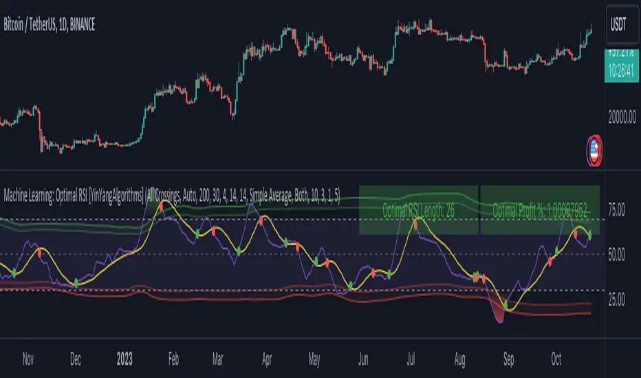
IPDA Standard Deviations [DexterLab x TFO x toodegrees]> Introduction and Acknowledgements
The IPDA Standard Deviations tool encompasses the Time and price relationship as studied by @TraderDext3r .
I am not the creator of this Theory, and I do not hold the answers to all the questions you may have; I suggest you to study it from Dexter's tweets, videos, and material.
This tool was born from a collaboration between @TraderDext3r, @tradeforopp and I, with the objective of bringing a comprehensive IPDA Standard Deviations tool to Tradingview.
> Tool Description
This is purely a graphical aid for traders to be able to quickly determine Fractal IPDA Time Windows, and trace the potential Standard Deviations of the moves at their respective high and low extremes.
The disruptive value of this tool is that it allows traders to save Time by automatically adapting the Time Windows based on the current chart's Timeframe, as well as providing customizations to filter and focus on the appropriate Standard Deviations.
> IPDA Standard Deviations by TraderDext3r
The underlying idea is based on the Interbank Price Delivery Algorithm's lookback windows on the daily chart as taught by the Inner Circle Trader:
IPDA looks at the past three months of price action to determine how to deliver price in the future.
Additionally, the ICT concept of projecting specific manipulation moves prior to large displacement upwards/downwards is used to navigate and interpret the priorly mentioned displacement move. We pay attention to specific Standard Deviations based on the current environment and overall narrative.
Dexter being one of the most prominent Inner Circle Trader students, harnessed the fractal nature of price to derive fractal IPDA Lookback Time Windows for lower Timeframes, and studied the behaviour of price at specific Deviations.
For Example:
The -1 to -2 area can initiate an algorithmic retracement before continuation.
The -2 to -2.5 area can initiate an algorithmic retracement before continuation, or a Smart Money Reversal.
The -4 area should be seen as the ultimate objective, or the level at which the displacement will slow down.
Given that these ideas stem from ICT's concepts themselves, they are to be used hand in hand with all other ICT Concepts (PD Array Matrix, PO3, Institutional Price Levels, ...).
> Fractal IPDA Time Windows
The IPDA Lookbacks Types identified by Dexter are as follows:
Monthly – 1D Chart: one widow per Month, highlighting the past three Months.
Weekly – 4H to 8H Chart: one window per Week, highlighting the past three Weeks.
Daily – 15m to 1H Chart: one window per Day, highlighting the past three Days.
Intraday – 1m to 5m Chart: one window per 4 Hours highlighting the past 12 Hours.
Inside these three respective Time Windows, the extreme High and Low will be identified, as well as the prior opposing short term market structure point. These represent the anchors for the Standard Deviation Projections.
> Tool Settings
The User is able to plot any type of Standard Deviation they want by inputting them in the settings, in their own line of the text box. They will always be plotted from the Time Windows extremes.
As previously mentioned, the User is also able to define their own Timeframe intervals for the respective IPDA Lookback Types. The specific Timeframes on which the different Lookback Types are plotted are edge-inclusive. In case of an overlap, the higher Timeframe Lookback will be prioritized.
Finally the User is able to filter and remove Standard Deviations in two ways:
"Remove Once Invalidated" will automatically delete a Deviation once its outer anchor extreme is traded through.
Manual Toggles will allow to remove the Upward or Downward Deviation of each Time Window at the discretion of the User.
Major shoutout to Dexter and TFO for their Time, it was a pleasure to collaborate and create this tool with them.
GLGT!

GKD-B Multi-Ticker Baseline [Loxx]Giga Kaleidoscope GKD-B Multi-Ticker Baseline is a Baseline module included in Loxx's "Giga Kaleidoscope Modularized Trading System".
This is a special implementation of GKD-B Baseline that allows the trader to input multiple tickers to be passed onto a GKD-BT Multi-Ticker Backtest. This baseline can only be used with the GKD-BT Multi-Ticker Backtests.
GKD-B Multi-Ticker Baseline includes 64 different moving averages:
Adaptive Moving Average - AMA
ADXvma - Average Directional Volatility Moving Average
Ahrens Moving Average
Alexander Moving Average - ALXMA
Deviation Scaled Moving Average - DSMA
Donchian
Double Exponential Moving Average - DEMA
Double Smoothed Exponential Moving Average - DSEMA
Double Smoothed FEMA - DSFEMA
Double Smoothed Range Weighted EMA - DSRWEMA
Double Smoothed Wilders EMA - DSWEMA
Double Weighted Moving Average - DWMA
Ehlers Optimal Tracking Filter - EOTF
Exponential Moving Average - EMA
Fast Exponential Moving Average - FEMA
Fractal Adaptive Moving Average - FRAMA
Generalized DEMA - GDEMA
Generalized Double DEMA - GDDEMA
Hull Moving Average (Type 1) - HMA1
Hull Moving Average (Type 2) - HMA2
Hull Moving Average (Type 3) - HMA3
Hull Moving Average (Type 4) - HMA4
IE /2 - Early T3 by Tim Tilson
Integral of Linear Regression Slope - ILRS
Instantaneous Trendline
Kalman Filter
Kaufman Adaptive Moving Average - KAMA
Laguerre Filter
Leader Exponential Moving Average
Linear Regression Value - LSMA ( Least Squares Moving Average )
Linear Weighted Moving Average - LWMA
McGinley Dynamic
McNicholl EMA
Non-Lag Moving Average
Ocean NMA Moving Average - ONMAMA
One More Moving Average - OMA
Parabolic Weighted Moving Average
Probability Density Function Moving Average - PDFMA
Quadratic Regression Moving Average - QRMA
Regularized EMA - REMA
Range Weighted EMA - RWEMA
Recursive Moving Trendline
Simple Decycler - SDEC
Simple Jurik Moving Average - SJMA
Simple Moving Average - SMA
Sine Weighted Moving Average
Smoothed LWMA - SLWMA
Smoothed Moving Average - SMMA
Smoother
Super Smoother
T3
Three-pole Ehlers Butterworth
Three-pole Ehlers Smoother
Triangular Moving Average - TMA
Triple Exponential Moving Average - TEMA
Two-pole Ehlers Butterworth
Two-pole Ehlers smoother
Variable Index Dynamic Average - VIDYA
Variable Moving Average - VMA
Volume Weighted EMA - VEMA
Volume Weighted Moving Average - VWMA
Zero-Lag DEMA - Zero Lag Exponential Moving Average
Zero-Lag Moving Average
Zero Lag TEMA - Zero Lag Triple Exponential Moving Average
Adaptive Moving Average - AMA
The Adaptive Moving Average (AMA) is a moving average that changes its sensitivity to price moves depending on the calculated volatility. It becomes more sensitive during periods when the price is moving smoothly in a certain direction and becomes less sensitive when the price is volatile.
ADXvma - Average Directional Volatility Moving Average
Linnsoft's ADXvma formula is a volatility-based moving average, with the volatility being determined by the value of the ADX indicator.
The ADXvma has the SMA in Chande's CMO replaced with an EMA , it then uses a few more layers of EMA smoothing before the "Volatility Index" is calculated.
A side effect is, those additional layers slow down the ADXvma when you compare it to Chande's Variable Index Dynamic Average VIDYA .
The ADXVMA provides support during uptrends and resistance during downtrends and will stay flat for longer, but will create some of the most accurate market signals when it decides to move.
Ahrens Moving Average
Richard D. Ahrens's Moving Average promises "Smoother Data" that isn't influenced by the occasional price spike. It works by using the Open and the Close in his formula so that the only time the Ahrens Moving Average will change is when the candlestick is either making new highs or new lows.
Alexander Moving Average - ALXMA
This Moving Average uses an elaborate smoothing formula and utilizes a 7 period Moving Average. It corresponds to fitting a second-order polynomial to seven consecutive observations. This moving average is rarely used in trading but is interesting as this Moving Average has been applied to diffusion indexes that tend to be very volatile.
Deviation Scaled Moving Average - DSMA
The Deviation-Scaled Moving Average is a data smoothing technique that acts like an exponential moving average with a dynamic smoothing coefficient. The smoothing coefficient is automatically updated based on the magnitude of price changes. In the Deviation-Scaled Moving Average, the standard deviation from the mean is chosen to be the measure of this magnitude. The resulting indicator provides substantial smoothing of the data even when price changes are small while quickly adapting to these changes.
Donchian
Donchian Channels are three lines generated by moving average calculations that comprise an indicator formed by upper and lower bands around a midrange or median band. The upper band marks the highest price of a security over N periods while the lower band marks the lowest price of a security over N periods.
Double Exponential Moving Average - DEMA
The Double Exponential Moving Average ( DEMA ) combines a smoothed EMA and a single EMA to provide a low-lag indicator. It's primary purpose is to reduce the amount of "lagging entry" opportunities, and like all Moving Averages, the DEMA confirms uptrends whenever price crosses on top of it and closes above it, and confirms downtrends when the price crosses under it and closes below it - but with significantly less lag.
Double Smoothed Exponential Moving Average - DSEMA
The Double Smoothed Exponential Moving Average is a lot less laggy compared to a traditional EMA . It's also considered a leading indicator compared to the EMA , and is best utilized whenever smoothness and speed of reaction to market changes are required.
Double Smoothed FEMA - DSFEMA
Same as the Double Exponential Moving Average (DEMA), but uses a faster version of EMA for its calculation.
Double Smoothed Range Weighted EMA - DSRWEMA
Range weighted exponential moving average (EMA) is, unlike the "regular" range weighted average calculated in a different way. Even though the basis - the range weighting - is the same, the way how it is calculated is completely different. By definition this type of EMA is calculated as a ratio of EMA of price*weight / EMA of weight. And the results are very different and the two should be considered as completely different types of averages. The higher than EMA to price changes responsiveness when the ranges increase remains in this EMA too and in those cases this EMA is clearly leading the "regular" EMA. This version includes double smoothing.
Double Smoothed Wilders EMA - DSWEMA
Welles Wilder was frequently using one "special" case of EMA (Exponential Moving Average) that is due to that fact (that he used it) sometimes called Wilder's EMA. This version is adding double smoothing to Wilder's EMA in order to make it "faster" (it is more responsive to market prices than the original) and is still keeping very smooth values.
Double Weighted Moving Average - DWMA
Double weighted moving average is an LWMA (Linear Weighted Moving Average). Instead of doing one cycle for calculating the LWMA, the indicator is made to cycle the loop 2 times. That produces a smoother values than the original LWMA
Ehlers Optimal Tracking Filter - EOTF
The Elher's Optimum Tracking Filter quickly adjusts rapid shifts in the price and yet is relatively smooth when the price has a sideways action. The operation of this filter is similar to Kaufman’s Adaptive Moving
Average
Exponential Moving Average - EMA
The EMA places more significance on recent data points and moves closer to price than the SMA ( Simple Moving Average ). It reacts faster to volatility due to its emphasis on recent data and is known for its ability to give greater weight to recent and more relevant data. The EMA is therefore seen as an enhancement over the SMA .
Fast Exponential Moving Average - FEMA
An Exponential Moving Average with a short look-back period.
Fractal Adaptive Moving Average - FRAMA
The Fractal Adaptive Moving Average by John Ehlers is an intelligent adaptive Moving Average which takes the importance of price changes into account and follows price closely enough to display significant moves whilst remaining flat if price ranges. The FRAMA does this by dynamically adjusting the look-back period based on the market's fractal geometry.
Generalized DEMA - GDEMA
The double exponential moving average (DEMA), was developed by Patrick Mulloy in an attempt to reduce the amount of lag time found in traditional moving averages. It was first introduced in the February 1994 issue of the magazine Technical Analysis of Stocks & Commodities in Mulloy's article "Smoothing Data with Faster Moving Averages.". Instead of using fixed multiplication factor in the final DEMA formula, the generalized version allows you to change it. By varying the "volume factor" form 0 to 1 you apply different multiplications and thus producing DEMA with different "speed" - the higher the volume factor is the "faster" the DEMA will be (but also the slope of it will be less smooth). The volume factor is limited in the calculation to 1 since any volume factor that is larger than 1 is increasing the overshooting to the extent that some volume factors usage makes the indicator unusable.
Generalized Double DEMA - GDDEMA
The double exponential moving average (DEMA), was developed by Patrick Mulloy in an attempt to reduce the amount of lag time found in traditional moving averages. It was first introduced in the February 1994 issue of the magazine Technical Analysis of Stocks & Commodities in Mulloy's article "Smoothing Data with Faster Moving Averages''. This is an extension of the Generalized DEMA using Tim Tillsons (the inventor of T3) idea, and is using GDEMA of GDEMA for calculation (which is the "middle step" of T3 calculation). Since there are no versions showing that middle step, this version covers that too. The result is smoother than Generalized DEMA, but is less smooth than T3 - one has to do some experimenting in order to find the optimal way to use it, but in any case, since it is "faster" than the T3 (Tim Tillson T3) and still smooth, it looks like a good compromise between speed and smoothness.
Hull Moving Average (Type 1) - HMA1
Alan Hull's HMA makes use of weighted moving averages to prioritize recent values and greatly reduce lag whilst maintaining the smoothness of a traditional Moving Average. For this reason, it's seen as a well-suited Moving Average for identifying entry points. This version uses SMA for smoothing.
Hull Moving Average (Type 2) - HMA2
Alan Hull's HMA makes use of weighted moving averages to prioritize recent values and greatly reduce lag whilst maintaining the smoothness of a traditional Moving Average. For this reason, it's seen as a well-suited Moving Average for identifying entry points. This version uses EMA for smoothing.
Hull Moving Average (Type 3) - HMA3
Alan Hull's HMA makes use of weighted moving averages to prioritize recent values and greatly reduce lag whilst maintaining the smoothness of a traditional Moving Average. For this reason, it's seen as a well-suited Moving Average for identifying entry points. This version uses LWMA for smoothing.
Hull Moving Average (Type 4) - HMA4
Alan Hull's HMA makes use of weighted moving averages to prioritize recent values and greatly reduce lag whilst maintaining the smoothness of a traditional Moving Average. For this reason, it's seen as a well-suited Moving Average for identifying entry points. This version uses SMMA for smoothing.
IE /2 - Early T3 by Tim Tilson and T3 new
The T3 moving average is a type of technical indicator used in financial analysis to identify trends in price movements. It is similar to the Exponential Moving Average (EMA) and the Double Exponential Moving Average (DEMA), but uses a different smoothing algorithm.
The T3 moving average is calculated using a series of exponential moving averages that are designed to filter out noise and smooth the data. The resulting smoothed data is then weighted with a non-linear function to produce a final output that is more responsive to changes in trend direction.
The T3 moving average can be customized by adjusting the length of the moving average, as well as the weighting function used to smooth the data. It is commonly used in conjunction with other technical indicators as part of a larger trading strategy.
Integral of Linear Regression Slope - ILRS
A Moving Average where the slope of a linear regression line is simply integrated as it is fitted in a moving window of length N (natural numbers in maths) across the data. The derivative of ILRS is the linear regression slope. ILRS is not the same as a SMA ( Simple Moving Average ) of length N, which is actually the midpoint of the linear regression line as it moves across the data.
Instantaneous Trendline
The Instantaneous Trendline is created by removing the dominant cycle component from the price information which makes this Moving Average suitable for medium to long-term trading.
Kalman Filter
Kalman filter is an algorithm that uses a series of measurements observed over time, containing statistical noise and other inaccuracies. This means that the filter was originally designed to work with noisy data. Also, it is able to work with incomplete data. Another advantage is that it is designed for and applied in dynamic systems; our price chart belongs to such systems. This version is true to the original design of the trade-ready Kalman Filter where velocity is the triggering mechanism.
Kalman Filter is a more accurate smoothing/prediction algorithm than the moving average because it is adaptive: it accounts for estimation errors and tries to adjust its predictions from the information it learned in the previous stage. Theoretically, Kalman Filter consists of measurement and transition components.
Kaufman Adaptive Moving Average - KAMA
Developed by Perry Kaufman, Kaufman's Adaptive Moving Average (KAMA) is a moving average designed to account for market noise or volatility. KAMA will closely follow prices when the price swings are relatively small and the noise is low.
Laguerre Filter
The Laguerre Filter is a smoothing filter which is based on Laguerre polynomials. The filter requires the current price, three prior prices, a user defined factor called Alpha to fill its calculation.
Adjusting the Alpha coefficient is used to increase or decrease its lag and its smoothness.
Leader Exponential Moving Average
The Leader EMA was created by Giorgos E. Siligardos who created a Moving Average which was able to eliminate lag altogether whilst maintaining some smoothness. It was first described during his research paper "MACD Leader" where he applied this to the MACD to improve its signals and remove its lagging issue. This filter uses his leading MACD's "modified EMA" and can be used as a zero lag filter.
Linear Regression Value - LSMA ( Least Squares Moving Average )
LSMA as a Moving Average is based on plotting the end point of the linear regression line. It compares the current value to the prior value and a determination is made of a possible trend, eg. the linear regression line is pointing up or down.
Linear Weighted Moving Average - LWMA
LWMA reacts to price quicker than the SMA and EMA . Although it's similar to the Simple Moving Average , the difference is that a weight coefficient is multiplied to the price which means the most recent price has the highest weighting, and each prior price has progressively less weight. The weights drop in a linear fashion.
McGinley Dynamic
John McGinley created this Moving Average to track prices better than traditional Moving Averages. It does this by incorporating an automatic adjustment factor into its formula, which speeds (or slows) the indicator in trending, or ranging, markets.
McNicholl EMA
Dennis McNicholl developed this Moving Average to use as his center line for his "Better Bollinger Bands" indicator and was successful because it responded better to volatility changes over the standard SMA and managed to avoid common whipsaws.
Non-lag moving average
The Non Lag Moving average follows price closely and gives very quick signals as well as early signals of price change. As a standalone Moving Average, it should not be used on its own, but as an additional confluence tool for early signals.
Ocean NMA Moving Average - ONMAMA
Created by Jim Sloman, the NMA is a moving average that automatically adjusts to volatility without being programmed to do so. For more info, read his guide "Ocean Theory, an Introduction"
One More Moving Average (OMA)
The One More Moving Average (OMA) is a technical indicator that calculates a series of Jurik-style moving averages in order to reduce noise and provide smoother price data. It uses six exponential moving averages to generate the final value, with the length of the moving averages determined by an adaptive algorithm that adjusts to the current market conditions. The algorithm calculates the average period by comparing the signal to noise ratio and using this value to determine the length of the moving averages. The resulting values are used to generate the final value of the OMA, which can be used to identify trends and potential changes in trend direction.
Parabolic Weighted Moving Average
The Parabolic Weighted Moving Average is a variation of the Linear Weighted Moving Average . The Linear Weighted Moving Average calculates the average by assigning different weights to each element in its calculation. The Parabolic Weighted Moving Average is a variation that allows weights to be changed to form a parabolic curve. It is done simply by using the Power parameter of this indicator.
Probability Density Function Moving Average - PDFMA
Probability density function based MA is a sort of weighted moving average that uses probability density function to calculate the weights. By its nature it is similar to a lot of digital filters.
Quadratic Regression Moving Average - QRMA
A quadratic regression is the process of finding the equation of the parabola that best fits a set of data. This moving average is an obscure concept that was posted to Forex forums in around 2008.
Regularized EMA - REMA
The regularized exponential moving average (REMA) by Chris Satchwell is a variation on the EMA (see Exponential Moving Average) designed to be smoother but not introduce too much extra lag.
Range Weighted EMA - RWEMA
This indicator is a variation of the range weighted EMA. The variation comes from a possible need to make that indicator a bit less "noisy" when it comes to slope changes. The method used for calculating this variation is the method described by Lee Leibfarth in his article "Trading With An Adaptive Price Zone".
Recursive Moving Trendline
Dennis Meyers's Recursive Moving Trendline uses a recursive (repeated application of a rule) polynomial fit, a technique that uses a small number of past values estimations of price and today's price to predict tomorrow's price.
Simple Decycler - SDEC
The Ehlers Simple Decycler study is a virtually zero-lag technical indicator proposed by John F. Ehlers. The original idea behind this study (and several others created by John F. Ehlers) is that market data can be considered a continuum of cycle periods with different cycle amplitudes. Thus, trending periods can be considered segments of longer cycles, or, in other words, low-frequency segments. Applying the right filter might help identify these segments.
Simple Loxx Moving Average - SLMA
A three stage moving average combining an adaptive EMA, a Kalman Filter, and a Kauffman adaptive filter.
Simple Moving Average - SMA
The SMA calculates the average of a range of prices by adding recent prices and then dividing that figure by the number of time periods in the calculation average. It is the most basic Moving Average which is seen as a reliable tool for starting off with Moving Average studies. As reliable as it may be, the basic moving average will work better when it's enhanced into an EMA .
Sine Weighted Moving Average
The Sine Weighted Moving Average assigns the most weight at the middle of the data set. It does this by weighting from the first half of a Sine Wave Cycle and the most weighting is given to the data in the middle of that data set. The Sine WMA closely resembles the TMA (Triangular Moving Average).
Smoothed LWMA - SLWMA
A smoothed version of the LWMA
Smoothed Moving Average - SMMA
The Smoothed Moving Average is similar to the Simple Moving Average ( SMA ), but aims to reduce noise rather than reduce lag. SMMA takes all prices into account and uses a long lookback period. Due to this, it's seen as an accurate yet laggy Moving Average.
Smoother
The Smoother filter is a faster-reacting smoothing technique which generates considerably less lag than the SMMA ( Smoothed Moving Average ). It gives earlier signals but can also create false signals due to its earlier reactions. This filter is sometimes wrongly mistaken for the superior Jurik Smoothing algorithm.
Super Smoother
The Super Smoother filter uses John Ehlers’s “Super Smoother” which consists of a Two pole Butterworth filter combined with a 2-bar SMA ( Simple Moving Average ) that suppresses the 22050 Hz Nyquist frequency: A characteristic of a sampler, which converts a continuous function or signal into a discrete sequence.
Three-pole Ehlers Butterworth
The 3 pole Ehlers Butterworth (as well as the Two pole Butterworth) are both superior alternatives to the EMA and SMA . They aim at producing less lag whilst maintaining accuracy. The 2 pole filter will give you a better approximation for price, whereas the 3 pole filter has superior smoothing.
Three-pole Ehlers smoother
The 3 pole Ehlers smoother works almost as close to price as the above mentioned 3 Pole Ehlers Butterworth. It acts as a strong baseline for signals but removes some noise. Side by side, it hardly differs from the Three Pole Ehlers Butterworth but when examined closely, it has better overshoot reduction compared to the 3 pole Ehlers Butterworth.
Triangular Moving Average - TMA
The TMA is similar to the EMA but uses a different weighting scheme. Exponential and weighted Moving Averages will assign weight to the most recent price data. Simple moving averages will assign the weight equally across all the price data. With a TMA (Triangular Moving Average), it is double smoother (averaged twice) so the majority of the weight is assigned to the middle portion of the data.
Triple Exponential Moving Average - TEMA
The TEMA uses multiple EMA calculations as well as subtracting lag to create a tool which can be used for scalping pullbacks. As it follows price closely, its signals are considered very noisy and should only be used in extremely fast-paced trading conditions.
Two-pole Ehlers Butterworth
The 2 pole Ehlers Butterworth (as well as the three pole Butterworth mentioned above) is another filter that cuts out the noise and follows the price closely. The 2 pole is seen as a faster, leading filter over the 3 pole and follows price a bit more closely. Analysts will utilize both a 2 pole and a 3 pole Butterworth on the same chart using the same period, but having both on chart allows its crosses to be traded.
Two-pole Ehlers smoother
A smoother version of the Two pole Ehlers Butterworth. This filter is the faster version out of the 3 pole Ehlers Butterworth. It does a decent job at cutting out market noise whilst emphasizing a closer following to price over the 3 pole Ehlers .
Variable Index Dynamic Average - VIDYA
Variable Index Dynamic Average Technical Indicator ( VIDYA ) was developed by Tushar Chande. It is an original method of calculating the Exponential Moving Average ( EMA ) with the dynamically changing period of averaging.
Variable Moving Average - VMA
The Variable Moving Average (VMA) is a study that uses an Exponential Moving Average being able to automatically adjust its smoothing factor according to the market volatility.
Volume Weighted EMA - VEMA
An EMA that uses a volume and price weighted calculation instead of the standard price input.
Volume Weighted Moving Average - VWMA
A Volume Weighted Moving Average is a moving average where more weight is given to bars with heavy volume than with light volume. Thus the value of the moving average will be closer to where most trading actually happened than it otherwise would be without being volume weighted.
Zero-Lag DEMA - Zero Lag Double Exponential Moving Average
John Ehlers's Zero Lag DEMA's aim is to eliminate the inherent lag associated with all trend following indicators which average a price over time. Because this is a Double Exponential Moving Average with Zero Lag, it has a tendency to overshoot and create a lot of false signals for swing trading. It can however be used for quick scalping or as a secondary indicator for confluence.
Zero-Lag Moving Average
The Zero Lag Moving Average is described by its creator, John Ehlers , as a Moving Average with absolutely no delay. And it's for this reason that this filter will cause a lot of abrupt signals which will not be ideal for medium to long-term traders. This filter is designed to follow price as close as possible whilst de-lagging data instead of basing it on regular data. The way this is done is by attempting to remove the cumulative effect of the Moving Average.
Zero-Lag TEMA - Zero Lag Triple Exponential Moving Average
Just like the Zero Lag DEMA , this filter will give you the fastest signals out of all the Zero Lag Moving Averages. This is useful for scalping but dangerous for medium to long-term traders, especially during market Volatility and news events. Having no lag, this filter also has no smoothing in its signals and can cause some very bizarre behavior when applied to certain indicators.
█ Volatility Goldie Locks Zone
This volatility filter is the standard first pass filter that is used for all NNFX systems despite the additional volatility/volume filter used in step 5. For this filter, price must fall into a range of maximum and minimum values calculated using multiples of volatility. Unlike the standard NNFX systems, this version of volatility filtering is separated from the core Baseline and uses it's own moving average with Loxx's Exotic Source Types.
█ Volatility Types included
The GKD system utilizes volatility-based take profits and stop losses. Each take profit and stop loss is calculated as a multiple of volatility. You can change the values of the multipliers in the settings as well.
This module includes 17 types of volatility:
Close-to-Close
Parkinson
Garman-Klass
Rogers-Satchell
Yang-Zhang
Garman-Klass-Yang-Zhang
Exponential Weighted Moving Average
Standard Deviation of Log Returns
Pseudo GARCH(2,2)
Average True Range
True Range Double
Standard Deviation
Adaptive Deviation
Median Absolute Deviation
Efficiency-Ratio Adaptive ATR
Mean Absolute Deviation
Static Percent
Various volatility estimators and indicators that investors and traders can use to measure the dispersion or volatility of a financial instrument's price. Each estimator has its strengths and weaknesses, and the choice of estimator should depend on the specific needs and circumstances of the user.
Close-to-Close
Close-to-Close volatility is a classic and widely used volatility measure, sometimes referred to as historical volatility.
Volatility is an indicator of the speed of a stock price change. A stock with high volatility is one where the price changes rapidly and with a larger amplitude. The more volatile a stock is, the riskier it is.
Close-to-close historical volatility is calculated using only a stock's closing prices. It is the simplest volatility estimator. However, in many cases, it is not precise enough. Stock prices could jump significantly during a trading session and return to the opening value at the end. That means that a considerable amount of price information is not taken into account by close-to-close volatility.
Despite its drawbacks, Close-to-Close volatility is still useful in cases where the instrument doesn't have intraday prices. For example, mutual funds calculate their net asset values daily or weekly, and thus their prices are not suitable for more sophisticated volatility estimators.
Parkinson
Parkinson volatility is a volatility measure that uses the stock’s high and low price of the day.
The main difference between regular volatility and Parkinson volatility is that the latter uses high and low prices for a day, rather than only the closing price. This is useful as close-to-close prices could show little difference while large price movements could have occurred during the day. Thus, Parkinson's volatility is considered more precise and requires less data for calculation than close-to-close volatility.
One drawback of this estimator is that it doesn't take into account price movements after the market closes. Hence, it systematically undervalues volatility. This drawback is addressed in the Garman-Klass volatility estimator.
Garman-Klass
Garman-Klass is a volatility estimator that incorporates open, low, high, and close prices of a security.
Garman-Klass volatility extends Parkinson's volatility by taking into account the opening and closing prices. As markets are most active during the opening and closing of a trading session, it makes volatility estimation more accurate.
Garman and Klass also assumed that the process of price change follows a continuous diffusion process (Geometric Brownian motion). However, this assumption has several drawbacks. The method is not robust for opening jumps in price and trend movements.
Despite its drawbacks, the Garman-Klass estimator is still more effective than the basic formula since it takes into account not only the price at the beginning and end of the time interval but also intraday price extremes.
Researchers Rogers and Satchell have proposed a more efficient method for assessing historical volatility that takes into account price trends. See Rogers-Satchell Volatility for more detail.
Rogers-Satchell
Rogers-Satchell is an estimator for measuring the volatility of securities with an average return not equal to zero.
Unlike Parkinson and Garman-Klass estimators, Rogers-Satchell incorporates a drift term (mean return not equal to zero). As a result, it provides better volatility estimation when the underlying is trending.
The main disadvantage of this method is that it does not take into account price movements between trading sessions. This leads to an underestimation of volatility since price jumps periodically occur in the market precisely at the moments between sessions.
A more comprehensive estimator that also considers the gaps between sessions was developed based on the Rogers-Satchel formula in the 2000s by Yang-Zhang. See Yang Zhang Volatility for more detail.
Yang-Zhang
Yang Zhang is a historical volatility estimator that handles both opening jumps and the drift and has a minimum estimation error.
Yang-Zhang volatility can be thought of as a combination of the overnight (close-to-open volatility) and a weighted average of the Rogers-Satchell volatility and the day’s open-to-close volatility. It is considered to be 14 times more efficient than the close-to-close estimator.
Garman-Klass-Yang-Zhang
Garman-Klass-Yang-Zhang (GKYZ) volatility estimator incorporates the returns of open, high, low, and closing prices in its calculation.
GKYZ volatility estimator takes into account overnight jumps but not the trend, i.e., it assumes that the underlying asset follows a Geometric Brownian Motion (GBM) process with zero drift. Therefore, the GKYZ volatility estimator tends to overestimate the volatility when the drift is different from zero. However, for a GBM process, this estimator is eight times more efficient than the close-to-close volatility estimator.
Exponential Weighted Moving Average
The Exponentially Weighted Moving Average (EWMA) is a quantitative or statistical measure used to model or describe a time series. The EWMA is widely used in finance, with the main applications being technical analysis and volatility modeling.
The moving average is designed such that older observations are given lower weights. The weights decrease exponentially as the data point gets older – hence the name exponentially weighted.
The only decision a user of the EWMA must make is the parameter lambda. The parameter decides how important the current observation is in the calculation of the EWMA. The higher the value of lambda, the more closely the EWMA tracks the original time series.
Standard Deviation of Log Returns
This is the simplest calculation of volatility. It's the standard deviation of ln(close/close(1)).
Pseudo GARCH(2,2)
This is calculated using a short- and long-run mean of variance multiplied by ?.
?avg(var;M) + (1 ? ?) avg(var;N) = 2?var/(M+1-(M-1)L) + 2(1-?)var/(M+1-(M-1)L)
Solving for ? can be done by minimizing the mean squared error of estimation; that is, regressing L^-1var - avg(var; N) against avg(var; M) - avg(var; N) and using the resulting beta estimate as ?.
Average True Range
The average true range (ATR) is a technical analysis indicator, introduced by market technician J. Welles Wilder Jr. in his book New Concepts in Technical Trading Systems, that measures market volatility by decomposing the entire range of an asset price for that period.
The true range indicator is taken as the greatest of the following: current high less the current low; the absolute value of the current high less the previous close; and the absolute value of the current low less the previous close. The ATR is then a moving average, generally using 14 days, of the true ranges.
True Range Double
A special case of ATR that attempts to correct for volatility skew.
Standard Deviation
Standard deviation is a statistic that measures the dispersion of a dataset relative to its mean and is calculated as the square root of the variance. The standard deviation is calculated as the square root of variance by determining each data point's deviation relative to the mean. If the data points are further from the mean, there is a higher deviation within the data set; thus, the more spread out the data, the higher the standard deviation.
Adaptive Deviation
By definition, the Standard Deviation (STD, also represented by the Greek letter sigma ? or the Latin letter s) is a measure that is used to quantify the amount of variation or dispersion of a set of data values. In technical analysis, we usually use it to measure the level of current volatility.
Standard Deviation is based on Simple Moving Average calculation for mean value. This version of standard deviation uses the properties of EMA to calculate what can be called a new type of deviation, and since it is based on EMA, we can call it EMA deviation. Additionally, Perry Kaufman's efficiency ratio is used to make it adaptive (since all EMA type calculations are nearly perfect for adapting).
The difference when compared to the standard is significant--not just because of EMA usage, but the efficiency ratio makes it a "bit more logical" in very volatile market conditions.
Median Absolute Deviation
The median absolute deviation is a measure of statistical dispersion. Moreover, the MAD is a robust statistic, being more resilient to outliers in a data set than the standard deviation. In the standard deviation, the distances from the mean are squared, so large deviations are weighted more heavily, and thus outliers can heavily influence it. In the MAD, the deviations of a small number of outliers are irrelevant.
Because the MAD is a more robust estimator of scale than the sample variance or standard deviation, it works better with distributions without a mean or variance, such as the Cauchy distribution.
For this indicator, a manual recreation of the quantile function in Pine Script is used. This is so users have a full inside view into how this is calculated.
Efficiency-Ratio Adaptive ATR
Average True Range (ATR) is a widely used indicator for many occasions in technical analysis. It is calculated as the RMA of the true range. This version adds a "twist": it uses Perry Kaufman's Efficiency Ratio to calculate adaptive true range.
Mean Absolute Deviation
The mean absolute deviation (MAD) is a measure of variability that indicates the average distance between observations and their mean. MAD uses the original units of the data, which simplifies interpretation. Larger values signify that the data points spread out further from the average. Conversely, lower values correspond to data points bunching closer to it. The mean absolute deviation is also known as the mean deviation and average absolute deviation.
This definition of the mean absolute deviation sounds similar to the standard deviation (SD). While both measure variability, they have different calculations. In recent years, some proponents of MAD have suggested that it replace the SD as the primary measure because it is a simpler concept that better fits real life.
█ Giga Kaleidoscope Modularized Trading System
Core components of an NNFX algorithmic trading strategy
The NNFX algorithm is built on the principles of trend, momentum, and volatility. There are six core components in the NNFX trading algorithm:
1. Volatility - price volatility; e.g., Average True Range, True Range Double, Close-to-Close, etc.
2. Baseline - a moving average to identify price trend
3. Confirmation 1 - a technical indicator used to identify trends
4. Confirmation 2 - a technical indicator used to identify trends
5. Continuation - a technical indicator used to identify trends
6. Volatility/Volume - a technical indicator used to identify volatility/volume breakouts/breakdown
7. Exit - a technical indicator used to determine when a trend is exhausted
8. Metamorphosis - a technical indicator that produces a compound signal from the combination of other GKD indicators*
*(not part of the NNFX algorithm)
What is Volatility in the NNFX trading system?
In the NNFX (No Nonsense Forex) trading system, ATR (Average True Range) is typically used to measure the volatility of an asset. It is used as a part of the system to help determine the appropriate stop loss and take profit levels for a trade. ATR is calculated by taking the average of the true range values over a specified period.
True range is calculated as the maximum of the following values:
-Current high minus the current low
-Absolute value of the current high minus the previous close
-Absolute value of the current low minus the previous close
ATR is a dynamic indicator that changes with changes in volatility. As volatility increases, the value of ATR increases, and as volatility decreases, the value of ATR decreases. By using ATR in NNFX system, traders can adjust their stop loss and take profit levels according to the volatility of the asset being traded. This helps to ensure that the trade is given enough room to move, while also minimizing potential losses.
Other types of volatility include True Range Double (TRD), Close-to-Close, and Garman-Klass
What is a Baseline indicator?
The baseline is essentially a moving average, and is used to determine the overall direction of the market.
The baseline in the NNFX system is used to filter out trades that are not in line with the long-term trend of the market. The baseline is plotted on the chart along with other indicators, such as the Moving Average (MA), the Relative Strength Index (RSI), and the Average True Range (ATR).
Trades are only taken when the price is in the same direction as the baseline. For example, if the baseline is sloping upwards, only long trades are taken, and if the baseline is sloping downwards, only short trades are taken. This approach helps to ensure that trades are in line with the overall trend of the market, and reduces the risk of entering trades that are likely to fail.
By using a baseline in the NNFX system, traders can have a clear reference point for determining the overall trend of the market, and can make more informed trading decisions. The baseline helps to filter out noise and false signals, and ensures that trades are taken in the direction of the long-term trend.
What is a Confirmation indicator?
Confirmation indicators are technical indicators that are used to confirm the signals generated by primary indicators. Primary indicators are the core indicators used in the NNFX system, such as the Average True Range (ATR), the Moving Average (MA), and the Relative Strength Index (RSI).
The purpose of the confirmation indicators is to reduce false signals and improve the accuracy of the trading system. They are designed to confirm the signals generated by the primary indicators by providing additional information about the strength and direction of the trend.
Some examples of confirmation indicators that may be used in the NNFX system include the Bollinger Bands, the MACD (Moving Average Convergence Divergence), and the MACD Oscillator. These indicators can provide information about the volatility, momentum, and trend strength of the market, and can be used to confirm the signals generated by the primary indicators.
In the NNFX system, confirmation indicators are used in combination with primary indicators and other filters to create a trading system that is robust and reliable. By using multiple indicators to confirm trading signals, the system aims to reduce the risk of false signals and improve the overall profitability of the trades.
What is a Continuation indicator?
In the NNFX (No Nonsense Forex) trading system, a continuation indicator is a technical indicator that is used to confirm a current trend and predict that the trend is likely to continue in the same direction. A continuation indicator is typically used in conjunction with other indicators in the system, such as a baseline indicator, to provide a comprehensive trading strategy.
What is a Volatility/Volume indicator?
Volume indicators, such as the On Balance Volume (OBV), the Chaikin Money Flow (CMF), or the Volume Price Trend (VPT), are used to measure the amount of buying and selling activity in a market. They are based on the trading volume of the market, and can provide information about the strength of the trend. In the NNFX system, volume indicators are used to confirm trading signals generated by the Moving Average and the Relative Strength Index. Volatility indicators include Average Direction Index, Waddah Attar, and Volatility Ratio. In the NNFX trading system, volatility is a proxy for volume and vice versa.
By using volume indicators as confirmation tools, the NNFX trading system aims to reduce the risk of false signals and improve the overall profitability of trades. These indicators can provide additional information about the market that is not captured by the primary indicators, and can help traders to make more informed trading decisions. In addition, volume indicators can be used to identify potential changes in market trends and to confirm the strength of price movements.
What is an Exit indicator?
The exit indicator is used in conjunction with other indicators in the system, such as the Moving Average (MA), the Relative Strength Index (RSI), and the Average True Range (ATR), to provide a comprehensive trading strategy.
The exit indicator in the NNFX system can be any technical indicator that is deemed effective at identifying optimal exit points. Examples of exit indicators that are commonly used include the Parabolic SAR, the Average Directional Index (ADX), and the Chandelier Exit.
The purpose of the exit indicator is to identify when a trend is likely to reverse or when the market conditions have changed, signaling the need to exit a trade. By using an exit indicator, traders can manage their risk and prevent significant losses.
In the NNFX system, the exit indicator is used in conjunction with a stop loss and a take profit order to maximize profits and minimize losses. The stop loss order is used to limit the amount of loss that can be incurred if the trade goes against the trader, while the take profit order is used to lock in profits when the trade is moving in the trader's favor.
Overall, the use of an exit indicator in the NNFX trading system is an important component of a comprehensive trading strategy. It allows traders to manage their risk effectively and improve the profitability of their trades by exiting at the right time.
What is an Metamorphosis indicator?
The concept of a metamorphosis indicator involves the integration of two or more GKD indicators to generate a compound signal. This is achieved by evaluating the accuracy of each indicator and selecting the signal from the indicator with the highest accuracy. As an illustration, let's consider a scenario where we calculate the accuracy of 10 indicators and choose the signal from the indicator that demonstrates the highest accuracy.
The resulting output from the metamorphosis indicator can then be utilized in a GKD-BT backtest by occupying a slot that aligns with the purpose of the metamorphosis indicator. The slot can be a GKD-B, GKD-C, or GKD-E slot, depending on the specific requirements and objectives of the indicator. This allows for seamless integration and utilization of the compound signal within the GKD-BT framework.
How does Loxx's GKD (Giga Kaleidoscope Modularized Trading System) implement the NNFX algorithm outlined above?
Loxx's GKD v2.0 system has five types of modules (indicators/strategies). These modules are:
1. GKD-BT - Backtesting module (Volatility, Number 1 in the NNFX algorithm)
2. GKD-B - Baseline module (Baseline and Volatility/Volume, Numbers 1 and 2 in the NNFX algorithm)
3. GKD-C - Confirmation 1/2 and Continuation module (Confirmation 1/2 and Continuation, Numbers 3, 4, and 5 in the NNFX algorithm)
4. GKD-V - Volatility/Volume module (Confirmation 1/2, Number 6 in the NNFX algorithm)
5. GKD-E - Exit module (Exit, Number 7 in the NNFX algorithm)
6. GKD-M - Metamorphosis module (Metamorphosis, Number 8 in the NNFX algorithm, but not part of the NNFX algorithm)
(additional module types will added in future releases)
Each module interacts with every module by passing data to A backtest module wherein the various components of the GKD system are combined to create a trading signal.
That is, the Baseline indicator passes its data to Volatility/Volume. The Volatility/Volume indicator passes its values to the Confirmation 1 indicator. The Confirmation 1 indicator passes its values to the Confirmation 2 indicator. The Confirmation 2 indicator passes its values to the Continuation indicator. The Continuation indicator passes its values to the Exit indicator, and finally, the Exit indicator passes its values to the Backtest strategy.
This chaining of indicators requires that each module conform to Loxx's GKD protocol, therefore allowing for the testing of every possible combination of technical indicators that make up the six components of the NNFX algorithm.
What does the application of the GKD trading system look like?
Example trading system:
Backtest: Multi-Ticker SCC Backtest
Baseline: Hull Moving Average
Volatility/Volume: Hurst Exponent
Confirmation 1: Fisher Trasnform
Confirmation 2: uf2018
Continuation: Vortex
Exit: Rex Oscillator
Metamorphosis: Baseline Optimizer
Each GKD indicator is denoted with a module identifier of either: GKD-BT, GKD-B, GKD-C, GKD-V, GKD-M, or GKD-E. This allows traders to understand to which module each indicator belongs and where each indicator fits into the GKD system.
█ Giga Kaleidoscope Modularized Trading System Signals
Standard Entry
1. GKD-C Confirmation gives signal
2. Baseline agrees
3. Price inside Goldie Locks Zone Minimum
4. Price inside Goldie Locks Zone Maximum
5. Confirmation 2 agrees
6. Volatility/Volume agrees
1-Candle Standard Entry
1a. GKD-C Confirmation gives signal
2a. Baseline agrees
3a. Price inside Goldie Locks Zone Minimum
4a. Price inside Goldie Locks Zone Maximum
Next Candle
1b. Price retraced
2b. Baseline agrees
3b. Confirmation 1 agrees
4b. Confirmation 2 agrees
5b. Volatility/Volume agrees
Baseline Entry
1. GKD-B Basline gives signal
2. Confirmation 1 agrees
3. Price inside Goldie Locks Zone Minimum
4. Price inside Goldie Locks Zone Maximum
5. Confirmation 2 agrees
6. Volatility/Volume agrees
7. Confirmation 1 signal was less than 'Maximum Allowable PSBC Bars Back' prior
1-Candle Baseline Entry
1a. GKD-B Baseline gives signal
2a. Confirmation 1 agrees
3a. Price inside Goldie Locks Zone Minimum
4a. Price inside Goldie Locks Zone Maximum
5a. Confirmation 1 signal was less than 'Maximum Allowable PSBC Bars Back' prior
Next Candle
1b. Price retraced
2b. Baseline agrees
3b. Confirmation 1 agrees
4b. Confirmation 2 agrees
5b. Volatility/Volume agrees
Volatility/Volume Entry
1. GKD-V Volatility/Volume gives signal
2. Confirmation 1 agrees
3. Price inside Goldie Locks Zone Minimum
4. Price inside Goldie Locks Zone Maximum
5. Confirmation 2 agrees
6. Baseline agrees
7. Confirmation 1 signal was less than 7 candles prior
1-Candle Volatility/Volume Entry
1a. GKD-V Volatility/Volume gives signal
2a. Confirmation 1 agrees
3a. Price inside Goldie Locks Zone Minimum
4a. Price inside Goldie Locks Zone Maximum
5a. Confirmation 1 signal was less than 'Maximum Allowable PSVVC Bars Back' prior
Next Candle
1b. Price retraced
2b. Volatility/Volume agrees
3b. Confirmation 1 agrees
4b. Confirmation 2 agrees
5b. Baseline agrees
Confirmation 2 Entry
1. GKD-C Confirmation 2 gives signal
2. Confirmation 1 agrees
3. Price inside Goldie Locks Zone Minimum
4. Price inside Goldie Locks Zone Maximum
5. Volatility/Volume agrees
6. Baseline agrees
7. Confirmation 1 signal was less than 7 candles prior
1-Candle Confirmation 2 Entry
1a. GKD-C Confirmation 2 gives signal
2a. Confirmation 1 agrees
3a. Price inside Goldie Locks Zone Minimum
4a. Price inside Goldie Locks Zone Maximum
5a. Confirmation 1 signal was less than 'Maximum Allowable PSC2C Bars Back' prior
Next Candle
1b. Price retraced
2b. Confirmation 2 agrees
3b. Confirmation 1 agrees
4b. Volatility/Volume agrees
5b. Baseline agrees
PullBack Entry
1a. GKD-B Baseline gives signal
2a. Confirmation 1 agrees
3a. Price is beyond 1.0x Volatility of Baseline
Next Candle
1b. Price inside Goldie Locks Zone Minimum
2b. Price inside Goldie Locks Zone Maximum
3b. Confirmation 1 agrees
4b. Confirmation 2 agrees
5b. Volatility/Volume agrees
Continuation Entry
1. Standard Entry, 1-Candle Standard Entry, Baseline Entry, 1-Candle Baseline Entry, Volatility/Volume Entry, 1-Candle Volatility/Volume Entry, Confirmation 2 Entry, 1-Candle Confirmation 2 Entry, or Pullback entry triggered previously
2. Baseline hasn't crossed since entry signal trigger
4. Confirmation 1 agrees
5. Baseline agrees
6. Confirmation 2 agrees
█ Connecting to Backtests
All GKD indicators are chained indicators meaning you export the value of the indicators to specialized backtest to creat your GKD trading system. Each indicator contains a proprietary signal generation algo that will only work with GKD backtests. You can find these backtests using the links below.
GKD-BT Giga Confirmation Stack Backtest
GKD-BT Giga Stacks Backtest
GKD-BT Full Giga Kaleidoscope Backtest
GKD-BT Solo Confirmation Super Complex Backtest
GKD-BT Solo Confirmation Complex Backtest
GKD-BT Solo Confirmation Simple Backtest
GKD-M Baseline Optimizer
GKD-M Accuracy Alchemist

GKD-M Baseline Optimizer [Loxx]Giga Kaleidoscope GKD-M Baseline Optimizer is a Metamorphosis module included in Loxx's "Giga Kaleidoscope Modularized Trading System".
The Baseline Optimizer enables traders to backtest over 60 moving averages using variable period inputs. It then exports the baseline with the highest cumulative win rate per candle to any baseline-enabled GKD backtest. To perform the backtesting, the trader selects an initial period input (default is 60) and a skip value that increments the initial period input up to seven times. For instance, if a skip value of 5 is chosen, the Baseline Optimizer will run the backtest for the selected moving average on periods such as 60, 65, 70, 75, and so on, up to 90. If the user selects an initial period input of 45 and a skip value of 2, the Baseline Optimizer will conduct backtests for the chosen moving average on periods like 45, 47, 49, 51, and so forth, up to 57.
The Baseline Optimizer provides a table displaying the output of the backtests for a specified date range. The table output represents the cumulative win rate for the given date range.
On the Metamorphosis side of the Baseline Optimizer, a cumulative backtest is calculated for each candle within the date range. This means that each candle may exhibit a different distribution of period inputs with the highest win rate for a particular moving average. The Baseline Optimizer identifies the period input combination with the highest win rates for long and short positions and creates a win-rate adaptive long and short moving average chart. The moving average used for shorts differs from the moving average used for longs, and the moving average for each candle may vary from any other candle. This customized baseline can then be exported to all baseline-enabled GKD backtests.
The backtest employed in the Baseline Optimizer is a Solo Confirmation Simple, allowing only one take profit and one stop loss to be set.
Lastly, the Baseline Optimizer incorporates Goldie Locks Zone filtering, which can be utilized for signal generation in advanced GKD backtests.
█ Moving Averages included in the Baseline Optimizer
Adaptive Moving Average - AMA
ADXvma - Average Directional Volatility Moving Average
Ahrens Moving Average
Alexander Moving Average - ALXMA
Deviation Scaled Moving Average - DSMA
Donchian
Double Exponential Moving Average - DEMA
Double Smoothed Exponential Moving Average - DSEMA
Double Smoothed FEMA - DSFEMA
Double Smoothed Range Weighted EMA - DSRWEMA
Double Smoothed Wilders EMA - DSWEMA
Double Weighted Moving Average - DWMA
Exponential Moving Average - EMA
Fast Exponential Moving Average - FEMA
Fractal Adaptive Moving Average - FRAMA
Generalized DEMA - GDEMA
Generalized Double DEMA - GDDEMA
Hull Moving Average (Type 1) - HMA1
Hull Moving Average (Type 2) - HMA2
Hull Moving Average (Type 3) - HMA3
Hull Moving Average (Type 4) - HMA4
IE /2 - Early T3 by Tim Tilson
Integral of Linear Regression Slope - ILRS
Kaufman Adaptive Moving Average - KAMA
Leader Exponential Moving Average
Linear Regression Value - LSMA ( Least Squares Moving Average )
Linear Weighted Moving Average - LWMA
McGinley Dynamic
McNicholl EMA
Non-Lag Moving Average
Ocean NMA Moving Average - ONMAMA
One More Moving Average - OMA
Parabolic Weighted Moving Average
Probability Density Function Moving Average - PDFMA
Quadratic Regression Moving Average - QRMA
Regularized EMA - REMA
Range Weighted EMA - RWEMA
Recursive Moving Trendline
Simple Decycler - SDEC
Simple Jurik Moving Average - SJMA
Simple Moving Average - SMA
Sine Weighted Moving Average
Smoothed LWMA - SLWMA
Smoothed Moving Average - SMMA
Smoother
Super Smoother
T3
Three-pole Ehlers Butterworth
Three-pole Ehlers Smoother
Triangular Moving Average - TMA
Triple Exponential Moving Average - TEMA
Two-pole Ehlers Butterworth
Two-pole Ehlers smoother
Variable Index Dynamic Average - VIDYA
Variable Moving Average - VMA
Volume Weighted EMA - VEMA
Volume Weighted Moving Average - VWMA
Zero-Lag DEMA - Zero Lag Exponential Moving Average
Zero-Lag Moving Average
Zero Lag TEMA - Zero Lag Triple Exponential Moving Average
Adaptive Moving Average - AMA
The Adaptive Moving Average (AMA) is a moving average that changes its sensitivity to price moves depending on the calculated volatility. It becomes more sensitive during periods when the price is moving smoothly in a certain direction and becomes less sensitive when the price is volatile.
ADXvma - Average Directional Volatility Moving Average
Linnsoft's ADXvma formula is a volatility-based moving average, with the volatility being determined by the value of the ADX indicator.
The ADXvma has the SMA in Chande's CMO replaced with an EMA , it then uses a few more layers of EMA smoothing before the "Volatility Index" is calculated.
A side effect is, those additional layers slow down the ADXvma when you compare it to Chande's Variable Index Dynamic Average VIDYA .
The ADXVMA provides support during uptrends and resistance during downtrends and will stay flat for longer, but will create some of the most accurate market signals when it decides to move.
Ahrens Moving Average
Richard D. Ahrens's Moving Average promises "Smoother Data" that isn't influenced by the occasional price spike. It works by using the Open and the Close in his formula so that the only time the Ahrens Moving Average will change is when the candlestick is either making new highs or new lows.
Alexander Moving Average - ALXMA
This Moving Average uses an elaborate smoothing formula and utilizes a 7 period Moving Average. It corresponds to fitting a second-order polynomial to seven consecutive observations. This moving average is rarely used in trading but is interesting as this Moving Average has been applied to diffusion indexes that tend to be very volatile.
Deviation Scaled Moving Average - DSMA
The Deviation-Scaled Moving Average is a data smoothing technique that acts like an exponential moving average with a dynamic smoothing coefficient. The smoothing coefficient is automatically updated based on the magnitude of price changes. In the Deviation-Scaled Moving Average, the standard deviation from the mean is chosen to be the measure of this magnitude. The resulting indicator provides substantial smoothing of the data even when price changes are small while quickly adapting to these changes.
Donchian
Donchian Channels are three lines generated by moving average calculations that comprise an indicator formed by upper and lower bands around a midrange or median band. The upper band marks the highest price of a security over N periods while the lower band marks the lowest price of a security over N periods.
Double Exponential Moving Average - DEMA
The Double Exponential Moving Average ( DEMA ) combines a smoothed EMA and a single EMA to provide a low-lag indicator. It's primary purpose is to reduce the amount of "lagging entry" opportunities, and like all Moving Averages, the DEMA confirms uptrends whenever price crosses on top of it and closes above it, and confirms downtrends when the price crosses under it and closes below it - but with significantly less lag.
Double Smoothed Exponential Moving Average - DSEMA
The Double Smoothed Exponential Moving Average is a lot less laggy compared to a traditional EMA . It's also considered a leading indicator compared to the EMA , and is best utilized whenever smoothness and speed of reaction to market changes are required.
Double Smoothed FEMA - DSFEMA
Same as the Double Exponential Moving Average (DEMA), but uses a faster version of EMA for its calculation.
Double Smoothed Range Weighted EMA - DSRWEMA
Range weighted exponential moving average (EMA) is, unlike the "regular" range weighted average calculated in a different way. Even though the basis - the range weighting - is the same, the way how it is calculated is completely different. By definition this type of EMA is calculated as a ratio of EMA of price*weight / EMA of weight. And the results are very different and the two should be considered as completely different types of averages. The higher than EMA to price changes responsiveness when the ranges increase remains in this EMA too and in those cases this EMA is clearly leading the "regular" EMA. This version includes double smoothing.
Double Smoothed Wilders EMA - DSWEMA
Welles Wilder was frequently using one "special" case of EMA (Exponential Moving Average) that is due to that fact (that he used it) sometimes called Wilder's EMA. This version is adding double smoothing to Wilder's EMA in order to make it "faster" (it is more responsive to market prices than the original) and is still keeping very smooth values.
Double Weighted Moving Average - DWMA
Double weighted moving average is an LWMA (Linear Weighted Moving Average). Instead of doing one cycle for calculating the LWMA, the indicator is made to cycle the loop 2 times. That produces a smoother values than the original LWMA
Exponential Moving Average - EMA
The EMA places more significance on recent data points and moves closer to price than the SMA ( Simple Moving Average ). It reacts faster to volatility due to its emphasis on recent data and is known for its ability to give greater weight to recent and more relevant data. The EMA is therefore seen as an enhancement over the SMA .
Fast Exponential Moving Average - FEMA
An Exponential Moving Average with a short look-back period.
Fractal Adaptive Moving Average - FRAMA
The Fractal Adaptive Moving Average by John Ehlers is an intelligent adaptive Moving Average which takes the importance of price changes into account and follows price closely enough to display significant moves whilst remaining flat if price ranges. The FRAMA does this by dynamically adjusting the look-back period based on the market's fractal geometry.
Generalized DEMA - GDEMA
The double exponential moving average (DEMA), was developed by Patrick Mulloy in an attempt to reduce the amount of lag time found in traditional moving averages. It was first introduced in the February 1994 issue of the magazine Technical Analysis of Stocks & Commodities in Mulloy's article "Smoothing Data with Faster Moving Averages.". Instead of using fixed multiplication factor in the final DEMA formula, the generalized version allows you to change it. By varying the "volume factor" form 0 to 1 you apply different multiplications and thus producing DEMA with different "speed" - the higher the volume factor is the "faster" the DEMA will be (but also the slope of it will be less smooth). The volume factor is limited in the calculation to 1 since any volume factor that is larger than 1 is increasing the overshooting to the extent that some volume factors usage makes the indicator unusable.
Generalized Double DEMA - GDDEMA
The double exponential moving average (DEMA), was developed by Patrick Mulloy in an attempt to reduce the amount of lag time found in traditional moving averages. It was first introduced in the February 1994 issue of the magazine Technical Analysis of Stocks & Commodities in Mulloy's article "Smoothing Data with Faster Moving Averages''. This is an extension of the Generalized DEMA using Tim Tillsons (the inventor of T3) idea, and is using GDEMA of GDEMA for calculation (which is the "middle step" of T3 calculation). Since there are no versions showing that middle step, this version covers that too. The result is smoother than Generalized DEMA, but is less smooth than T3 - one has to do some experimenting in order to find the optimal way to use it, but in any case, since it is "faster" than the T3 (Tim Tillson T3) and still smooth, it looks like a good compromise between speed and smoothness.
Hull Moving Average (Type 1) - HMA1
Alan Hull's HMA makes use of weighted moving averages to prioritize recent values and greatly reduce lag whilst maintaining the smoothness of a traditional Moving Average. For this reason, it's seen as a well-suited Moving Average for identifying entry points. This version uses SMA for smoothing.
Hull Moving Average (Type 2) - HMA2
Alan Hull's HMA makes use of weighted moving averages to prioritize recent values and greatly reduce lag whilst maintaining the smoothness of a traditional Moving Average. For this reason, it's seen as a well-suited Moving Average for identifying entry points. This version uses EMA for smoothing.
Hull Moving Average (Type 3) - HMA3
Alan Hull's HMA makes use of weighted moving averages to prioritize recent values and greatly reduce lag whilst maintaining the smoothness of a traditional Moving Average. For this reason, it's seen as a well-suited Moving Average for identifying entry points. This version uses LWMA for smoothing.
Hull Moving Average (Type 4) - HMA4
Alan Hull's HMA makes use of weighted moving averages to prioritize recent values and greatly reduce lag whilst maintaining the smoothness of a traditional Moving Average. For this reason, it's seen as a well-suited Moving Average for identifying entry points. This version uses SMMA for smoothing.
IE /2 - Early T3 by Tim Tilson and T3 new
The T3 moving average is a type of technical indicator used in financial analysis to identify trends in price movements. It is similar to the Exponential Moving Average (EMA) and the Double Exponential Moving Average (DEMA), but uses a different smoothing algorithm.
The T3 moving average is calculated using a series of exponential moving averages that are designed to filter out noise and smooth the data. The resulting smoothed data is then weighted with a non-linear function to produce a final output that is more responsive to changes in trend direction.
The T3 moving average can be customized by adjusting the length of the moving average, as well as the weighting function used to smooth the data. It is commonly used in conjunction with other technical indicators as part of a larger trading strategy.
Integral of Linear Regression Slope - ILRS
A Moving Average where the slope of a linear regression line is simply integrated as it is fitted in a moving window of length N (natural numbers in maths) across the data. The derivative of ILRS is the linear regression slope. ILRS is not the same as a SMA ( Simple Moving Average ) of length N, which is actually the midpoint of the linear regression line as it moves across the data.
Kaufman Adaptive Moving Average - KAMA
Developed by Perry Kaufman, Kaufman's Adaptive Moving Average (KAMA) is a moving average designed to account for market noise or volatility. KAMA will closely follow prices when the price swings are relatively small and the noise is low.
Leader Exponential Moving Average
The Leader EMA was created by Giorgos E. Siligardos who created a Moving Average which was able to eliminate lag altogether whilst maintaining some smoothness. It was first described during his research paper "MACD Leader" where he applied this to the MACD to improve its signals and remove its lagging issue. This filter uses his leading MACD's "modified EMA" and can be used as a zero lag filter.
Linear Regression Value - LSMA ( Least Squares Moving Average )
LSMA as a Moving Average is based on plotting the end point of the linear regression line. It compares the current value to the prior value and a determination is made of a possible trend, eg. the linear regression line is pointing up or down.
Linear Weighted Moving Average - LWMA
LWMA reacts to price quicker than the SMA and EMA . Although it's similar to the Simple Moving Average , the difference is that a weight coefficient is multiplied to the price which means the most recent price has the highest weighting, and each prior price has progressively less weight. The weights drop in a linear fashion.
McGinley Dynamic
John McGinley created this Moving Average to track prices better than traditional Moving Averages. It does this by incorporating an automatic adjustment factor into its formula, which speeds (or slows) the indicator in trending, or ranging, markets.
McNicholl EMA
Dennis McNicholl developed this Moving Average to use as his center line for his "Better Bollinger Bands" indicator and was successful because it responded better to volatility changes over the standard SMA and managed to avoid common whipsaws.
Non-lag moving average
The Non Lag Moving average follows price closely and gives very quick signals as well as early signals of price change. As a standalone Moving Average, it should not be used on its own, but as an additional confluence tool for early signals.
Ocean NMA Moving Average - ONMAMA
Created by Jim Sloman, the NMA is a moving average that automatically adjusts to volatility without being programmed to do so. For more info, read his guide "Ocean Theory, an Introduction"
One More Moving Average (OMA)
The One More Moving Average (OMA) is a technical indicator that calculates a series of Jurik-style moving averages in order to reduce noise and provide smoother price data. It uses six exponential moving averages to generate the final value, with the length of the moving averages determined by an adaptive algorithm that adjusts to the current market conditions. The algorithm calculates the average period by comparing the signal to noise ratio and using this value to determine the length of the moving averages. The resulting values are used to generate the final value of the OMA, which can be used to identify trends and potential changes in trend direction.
Parabolic Weighted Moving Average
The Parabolic Weighted Moving Average is a variation of the Linear Weighted Moving Average . The Linear Weighted Moving Average calculates the average by assigning different weights to each element in its calculation. The Parabolic Weighted Moving Average is a variation that allows weights to be changed to form a parabolic curve. It is done simply by using the Power parameter of this indicator.
Probability Density Function Moving Average - PDFMA
Probability density function based MA is a sort of weighted moving average that uses probability density function to calculate the weights. By its nature it is similar to a lot of digital filters.
Quadratic Regression Moving Average - QRMA
A quadratic regression is the process of finding the equation of the parabola that best fits a set of data. This moving average is an obscure concept that was posted to Forex forums in around 2008.
Regularized EMA - REMA
The regularized exponential moving average (REMA) by Chris Satchwell is a variation on the EMA (see Exponential Moving Average) designed to be smoother but not introduce too much extra lag.
Range Weighted EMA - RWEMA
This indicator is a variation of the range weighted EMA. The variation comes from a possible need to make that indicator a bit less "noisy" when it comes to slope changes. The method used for calculating this variation is the method described by Lee Leibfarth in his article "Trading With An Adaptive Price Zone".
Recursive Moving Trendline
Dennis Meyers's Recursive Moving Trendline uses a recursive (repeated application of a rule) polynomial fit, a technique that uses a small number of past values estimations of price and today's price to predict tomorrow's price.
Simple Decycler - SDEC
The Ehlers Simple Decycler study is a virtually zero-lag technical indicator proposed by John F. Ehlers. The original idea behind this study (and several others created by John F. Ehlers) is that market data can be considered a continuum of cycle periods with different cycle amplitudes. Thus, trending periods can be considered segments of longer cycles, or, in other words, low-frequency segments. Applying the right filter might help identify these segments.
Simple Loxx Moving Average - SLMA
A three stage moving average combining an adaptive EMA, a Kalman Filter, and a Kauffman adaptive filter.
Simple Moving Average - SMA
The SMA calculates the average of a range of prices by adding recent prices and then dividing that figure by the number of time periods in the calculation average. It is the most basic Moving Average which is seen as a reliable tool for starting off with Moving Average studies. As reliable as it may be, the basic moving average will work better when it's enhanced into an EMA .
Sine Weighted Moving Average
The Sine Weighted Moving Average assigns the most weight at the middle of the data set. It does this by weighting from the first half of a Sine Wave Cycle and the most weighting is given to the data in the middle of that data set. The Sine WMA closely resembles the TMA (Triangular Moving Average).
Smoothed LWMA - SLWMA
A smoothed version of the LWMA
Smoothed Moving Average - SMMA
The Smoothed Moving Average is similar to the Simple Moving Average ( SMA ), but aims to reduce noise rather than reduce lag. SMMA takes all prices into account and uses a long lookback period. Due to this, it's seen as an accurate yet laggy Moving Average.
Smoother
The Smoother filter is a faster-reacting smoothing technique which generates considerably less lag than the SMMA ( Smoothed Moving Average ). It gives earlier signals but can also create false signals due to its earlier reactions. This filter is sometimes wrongly mistaken for the superior Jurik Smoothing algorithm.
Super Smoother
The Super Smoother filter uses John Ehlers’s “Super Smoother” which consists of a Two pole Butterworth filter combined with a 2-bar SMA ( Simple Moving Average ) that suppresses the 22050 Hz Nyquist frequency: A characteristic of a sampler, which converts a continuous function or signal into a discrete sequence.
Three-pole Ehlers Butterworth
The 3 pole Ehlers Butterworth (as well as the Two pole Butterworth) are both superior alternatives to the EMA and SMA . They aim at producing less lag whilst maintaining accuracy. The 2 pole filter will give you a better approximation for price, whereas the 3 pole filter has superior smoothing.
Three-pole Ehlers smoother
The 3 pole Ehlers smoother works almost as close to price as the above mentioned 3 Pole Ehlers Butterworth. It acts as a strong baseline for signals but removes some noise. Side by side, it hardly differs from the Three Pole Ehlers Butterworth but when examined closely, it has better overshoot reduction compared to the 3 pole Ehlers Butterworth.
Triangular Moving Average - TMA
The TMA is similar to the EMA but uses a different weighting scheme. Exponential and weighted Moving Averages will assign weight to the most recent price data. Simple moving averages will assign the weight equally across all the price data. With a TMA (Triangular Moving Average), it is double smoother (averaged twice) so the majority of the weight is assigned to the middle portion of the data.
Triple Exponential Moving Average - TEMA
The TEMA uses multiple EMA calculations as well as subtracting lag to create a tool which can be used for scalping pullbacks. As it follows price closely, its signals are considered very noisy and should only be used in extremely fast-paced trading conditions.
Two-pole Ehlers Butterworth
The 2 pole Ehlers Butterworth (as well as the three pole Butterworth mentioned above) is another filter that cuts out the noise and follows the price closely. The 2 pole is seen as a faster, leading filter over the 3 pole and follows price a bit more closely. Analysts will utilize both a 2 pole and a 3 pole Butterworth on the same chart using the same period, but having both on chart allows its crosses to be traded.
Two-pole Ehlers smoother
A smoother version of the Two pole Ehlers Butterworth. This filter is the faster version out of the 3 pole Ehlers Butterworth. It does a decent job at cutting out market noise whilst emphasizing a closer following to price over the 3 pole Ehlers .
Variable Index Dynamic Average - VIDYA
Variable Index Dynamic Average Technical Indicator ( VIDYA ) was developed by Tushar Chande. It is an original method of calculating the Exponential Moving Average ( EMA ) with the dynamically changing period of averaging.
Variable Moving Average - VMA
The Variable Moving Average (VMA) is a study that uses an Exponential Moving Average being able to automatically adjust its smoothing factor according to the market volatility.
Volume Weighted EMA - VEMA
An EMA that uses a volume and price weighted calculation instead of the standard price input.
Volume Weighted Moving Average - VWMA
A Volume Weighted Moving Average is a moving average where more weight is given to bars with heavy volume than with light volume. Thus the value of the moving average will be closer to where most trading actually happened than it otherwise would be without being volume weighted.
Zero-Lag DEMA - Zero Lag Double Exponential Moving Average
John Ehlers's Zero Lag DEMA's aim is to eliminate the inherent lag associated with all trend following indicators which average a price over time. Because this is a Double Exponential Moving Average with Zero Lag, it has a tendency to overshoot and create a lot of false signals for swing trading. It can however be used for quick scalping or as a secondary indicator for confluence.
Zero-Lag Moving Average
The Zero Lag Moving Average is described by its creator, John Ehlers , as a Moving Average with absolutely no delay. And it's for this reason that this filter will cause a lot of abrupt signals which will not be ideal for medium to long-term traders. This filter is designed to follow price as close as possible whilst de-lagging data instead of basing it on regular data. The way this is done is by attempting to remove the cumulative effect of the Moving Average.
Zero-Lag TEMA - Zero Lag Triple Exponential Moving Average
Just like the Zero Lag DEMA , this filter will give you the fastest signals out of all the Zero Lag Moving Averages. This is useful for scalping but dangerous for medium to long-term traders, especially during market Volatility and news events. Having no lag, this filter also has no smoothing in its signals and can cause some very bizarre behavior when applied to certain indicators.
█ Volatility Goldie Locks Zone
The Goldie Locks Zone volatility filter is the standard first-pass filter used in all advanced GKD backtests (Complex, Super Complex, and Full GKd). This filter requires the price to fall within a range determined by multiples of volatility. The Goldie Locks Zone is separate from the core Baseline and utilizes its own moving average with Loxx's Exotic Source Types you can read about below.
On the chart, you will find green and red dots positioned at the top, indicating whether a candle qualifies for a long or short trade respectively. Additionally, green and red triangles are located at the bottom of the chart, signifying whether the trigger has crossed up or down and qualifies within the Goldie Locks zone. The Goldie Locks zone is represented by a white color on the mean line, indicating low volatility levels that are not suitable for trading.
█ Volatility Types Included in the Baseline Optimizer
The GKD system utilizes volatility-based take profits and stop losses. Each take profit and stop loss is calculated as a multiple of volatility. Users can also adjust the multiplier values in the settings.
This module includes 17 types of volatility:
Close-to-Close
Parkinson
Garman-Klass
Rogers-Satchell
Yang-Zhang
Garman-Klass-Yang-Zhang
Exponential Weighted Moving Average
Standard Deviation of Log Returns
Pseudo GARCH(2,2)
Average True Range
True Range Double
Standard Deviation
Adaptive Deviation
Median Absolute Deviation
Efficiency-Ratio Adaptive ATR
Mean Absolute Deviation
Static Percent
Various volatility estimators and indicators that investors and traders can use to measure the dispersion or volatility of a financial instrument's price. Each estimator has its strengths and weaknesses, and the choice of estimator should depend on the specific needs and circumstances of the user.
Close-to-Close
Close-to-Close volatility is a classic and widely used volatility measure, sometimes referred to as historical volatility.
Volatility is an indicator of the speed of a stock price change. A stock with high volatility is one where the price changes rapidly and with a larger amplitude. The more volatile a stock is, the riskier it is.
Close-to-close historical volatility is calculated using only a stock's closing prices. It is the simplest volatility estimator. However, in many cases, it is not precise enough. Stock prices could jump significantly during a trading session and return to the opening value at the end. That means that a considerable amount of price information is not taken into account by close-to-close volatility.
Despite its drawbacks, Close-to-Close volatility is still useful in cases where the instrument doesn't have intraday prices. For example, mutual funds calculate their net asset values daily or weekly, and thus their prices are not suitable for more sophisticated volatility estimators.
Parkinson
Parkinson volatility is a volatility measure that uses the stock’s high and low price of the day.
The main difference between regular volatility and Parkinson volatility is that the latter uses high and low prices for a day, rather than only the closing price. This is useful as close-to-close prices could show little difference while large price movements could have occurred during the day. Thus, Parkinson's volatility is considered more precise and requires less data for calculation than close-to-close volatility.
One drawback of this estimator is that it doesn't take into account price movements after the market closes. Hence, it systematically undervalues volatility. This drawback is addressed in the Garman-Klass volatility estimator.
Garman-Klass
Garman-Klass is a volatility estimator that incorporates open, low, high, and close prices of a security.
Garman-Klass volatility extends Parkinson's volatility by taking into account the opening and closing prices. As markets are most active during the opening and closing of a trading session, it makes volatility estimation more accurate.
Garman and Klass also assumed that the process of price change follows a continuous diffusion process (Geometric Brownian motion). However, this assumption has several drawbacks. The method is not robust for opening jumps in price and trend movements.
Despite its drawbacks, the Garman-Klass estimator is still more effective than the basic formula since it takes into account not only the price at the beginning and end of the time interval but also intraday price extremes.
Researchers Rogers and Satchell have proposed a more efficient method for assessing historical volatility that takes into account price trends. See Rogers-Satchell Volatility for more detail.
Rogers-Satchell
Rogers-Satchell is an estimator for measuring the volatility of securities with an average return not equal to zero.
Unlike Parkinson and Garman-Klass estimators, Rogers-Satchell incorporates a drift term (mean return not equal to zero). As a result, it provides better volatility estimation when the underlying is trending.
The main disadvantage of this method is that it does not take into account price movements between trading sessions. This leads to an underestimation of volatility since price jumps periodically occur in the market precisely at the moments between sessions.
A more comprehensive estimator that also considers the gaps between sessions was developed based on the Rogers-Satchel formula in the 2000s by Yang-Zhang. See Yang Zhang Volatility for more detail.
Yang-Zhang
Yang Zhang is a historical volatility estimator that handles both opening jumps and the drift and has a minimum estimation error.
Yang-Zhang volatility can be thought of as a combination of the overnight (close-to-open volatility) and a weighted average of the Rogers-Satchell volatility and the day’s open-to-close volatility. It is considered to be 14 times more efficient than the close-to-close estimator.
Garman-Klass-Yang-Zhang
Garman-Klass-Yang-Zhang (GKYZ) volatility estimator incorporates the returns of open, high, low, and closing prices in its calculation.
GKYZ volatility estimator takes into account overnight jumps but not the trend, i.e., it assumes that the underlying asset follows a Geometric Brownian Motion (GBM) process with zero drift. Therefore, the GKYZ volatility estimator tends to overestimate the volatility when the drift is different from zero. However, for a GBM process, this estimator is eight times more efficient than the close-to-close volatility estimator.
Exponential Weighted Moving Average
The Exponentially Weighted Moving Average (EWMA) is a quantitative or statistical measure used to model or describe a time series. The EWMA is widely used in finance, with the main applications being technical analysis and volatility modeling.
The moving average is designed such that older observations are given lower weights. The weights decrease exponentially as the data point gets older – hence the name exponentially weighted.
The only decision a user of the EWMA must make is the parameter lambda. The parameter decides how important the current observation is in the calculation of the EWMA. The higher the value of lambda, the more closely the EWMA tracks the original time series.
Standard Deviation of Log Returns
This is the simplest calculation of volatility. It's the standard deviation of ln(close/close(1)).
Pseudo GARCH(2,2)
This is calculated using a short- and long-run mean of variance multiplied by ?.
?avg(var;M) + (1 ? ?) avg(var;N) = 2?var/(M+1-(M-1)L) + 2(1-?)var/(M+1-(M-1)L)
Solving for ? can be done by minimizing the mean squared error of estimation; that is, regressing L^-1var - avg(var; N) against avg(var; M) - avg(var; N) and using the resulting beta estimate as ?.
Average True Range
The average true range (ATR) is a technical analysis indicator, introduced by market technician J. Welles Wilder Jr. in his book New Concepts in Technical Trading Systems, that measures market volatility by decomposing the entire range of an asset price for that period.
The true range indicator is taken as the greatest of the following: current high less the current low; the absolute value of the current high less the previous close; and the absolute value of the current low less the previous close. The ATR is then a moving average, generally using 14 days, of the true ranges.
True Range Double
A special case of ATR that attempts to correct for volatility skew.
Standard Deviation
Standard deviation is a statistic that measures the dispersion of a dataset relative to its mean and is calculated as the square root of the variance. The standard deviation is calculated as the square root of variance by determining each data point's deviation relative to the mean. If the data points are further from the mean, there is a higher deviation within the data set; thus, the more spread out the data, the higher the standard deviation.
Adaptive Deviation
By definition, the Standard Deviation (STD, also represented by the Greek letter sigma ? or the Latin letter s) is a measure that is used to quantify the amount of variation or dispersion of a set of data values. In technical analysis, we usually use it to measure the level of current volatility.
Standard Deviation is based on Simple Moving Average calculation for mean value. This version of standard deviation uses the properties of EMA to calculate what can be called a new type of deviation, and since it is based on EMA, we can call it EMA deviation. Additionally, Perry Kaufman's efficiency ratio is used to make it adaptive (since all EMA type calculations are nearly perfect for adapting).
The difference when compared to the standard is significant--not just because of EMA usage, but the efficiency ratio makes it a "bit more logical" in very volatile market conditions.
Median Absolute Deviation
The median absolute deviation is a measure of statistical dispersion. Moreover, the MAD is a robust statistic, being more resilient to outliers in a data set than the standard deviation. In the standard deviation, the distances from the mean are squared, so large deviations are weighted more heavily, and thus outliers can heavily influence it. In the MAD, the deviations of a small number of outliers are irrelevant.
Because the MAD is a more robust estimator of scale than the sample variance or standard deviation, it works better with distributions without a mean or variance, such as the Cauchy distribution.
For this indicator, a manual recreation of the quantile function in Pine Script is used. This is so users have a full inside view into how this is calculated.
Efficiency-Ratio Adaptive ATR
Average True Range (ATR) is a widely used indicator for many occasions in technical analysis. It is calculated as the RMA of the true range. This version adds a "twist": it uses Perry Kaufman's Efficiency Ratio to calculate adaptive true range.
Mean Absolute Deviation
The mean absolute deviation (MAD) is a measure of variability that indicates the average distance between observations and their mean. MAD uses the original units of the data, which simplifies interpretation. Larger values signify that the data points spread out further from the average. Conversely, lower values correspond to data points bunching closer to it. The mean absolute deviation is also known as the mean deviation and average absolute deviation.
This definition of the mean absolute deviation sounds similar to the standard deviation (SD). While both measure variability, they have different calculations. In recent years, some proponents of MAD have suggested that it replace the SD as the primary measure because it is a simpler concept that better fits real life.
█ Loxx's Expanded Source Types Included in Baseline Optimizer
This indicator allows you to select from 33 source types. They are as follows:
Close
Open
High
Low
Median
Typical
Weighted
Average
Average Median Body
Trend Biased
Trend Biased (Extreme)
HA Close
HA Open
HA High
HA Low
HA Median
HA Typical
HA Weighted
HA Average
HA Average Median Body
HA Trend Biased
HA Trend Biased (Extreme)
HAB Close
HAB Open
HAB High
HAB Low
HAB Median
HAB Typical
HAB Weighted
HAB Average
HAB Average Median Body
HAB Trend Biased
HAB Trend Biased (Extreme)
What are Heiken Ashi "better" candles?
Heiken Ashi "better" candles are a modified version of the standard Heiken Ashi candles, which are a popular charting technique used in technical analysis. Heiken Ashi candles help traders identify trends and potential reversal points by smoothing out price data and reducing market noise. The "better formula" was proposed by Sebastian Schmidt in an article published by BNP Paribas in Warrants & Zertifikate, a German magazine, in August 2004. The aim of this formula is to further improve the smoothing of the Heiken Ashi chart and enhance its effectiveness in identifying trends and reversals.
Standard Heiken Ashi candles are calculated using the following formulas:
Heiken Ashi Close = (Open + High + Low + Close) / 4
Heiken Ashi Open = (Previous Heiken Ashi Open + Previous Heiken Ashi Close) / 2
Heiken Ashi High = Max (High, Heiken Ashi Open, Heiken Ashi Close)
Heiken Ashi Low = Min (Low, Heiken Ashi Open, Heiken Ashi Close)
The "better formula" modifies the standard Heiken Ashi calculation by incorporating additional smoothing, which can help reduce noise and make it easier to identify trends and reversals. The modified formulas for Heiken Ashi "better" candles are as follows:
Better Heiken Ashi Close = (Open + High + Low + Close) / 4
Better Heiken Ashi Open = (Previous Better Heiken Ashi Open + Previous Better Heiken Ashi Close) / 2
Better Heiken Ashi High = Max (High, Better Heiken Ashi Open, Better Heiken Ashi Close)
Better Heiken Ashi Low = Min (Low, Better Heiken Ashi Open, Better Heiken Ashi Close)
Smoothing Factor = 2 / (N + 1), where N is the chosen period for smoothing
Smoothed Better Heiken Ashi Open = (Better Heiken Ashi Open * Smoothing Factor) + (Previous Smoothed Better Heiken Ashi Open * (1 - Smoothing Factor))
Smoothed Better Heiken Ashi Close = (Better Heiken Ashi Close * Smoothing Factor) + (Previous Smoothed Better Heiken Ashi Close * (1 - Smoothing Factor))
The smoothed Better Heiken Ashi Open and Close values are then used to calculate the smoothed Better Heiken Ashi High and Low values, resulting in "better" candles that provide a clearer representation of the market trend and potential reversal points.
Heiken Ashi "better" candles, as mentioned previously, provide a clearer representation of market trends and potential reversal points by reducing noise and smoothing out price data. When using these candles in conjunction with other technical analysis tools and indicators, traders can gain valuable insights into market behavior and make more informed decisions.
To effectively use Heiken Ashi "better" candles in your trading strategy, consider the following tips:
-Trend Identification: Heiken Ashi "better" candles can help you identify the prevailing trend in the market. When the majority of the candles are green (or another color, depending on your chart settings) and there are no or few lower wicks, it may indicate a strong uptrend. Conversely, when the majority of the candles are red (or another color) and there are no or few upper wicks, it may signal a strong downtrend.
-Trend Reversals: Look for potential trend reversals when a change in the color of the candles occurs, especially when accompanied by longer wicks. For example, if a green candle with a long lower wick is followed by a red candle, it could indicate a bearish reversal. Similarly, a red candle with a long upper wick followed by a green candle may suggest a bullish reversal.
-Support and Resistance: You can use Heiken Ashi "better" candles to identify potential support and resistance levels. When the candles are consistently moving in one direction and then suddenly change color with longer wicks, it could indicate the presence of a support or resistance level.
-Stop-Loss and Take-Profit: Using Heiken Ashi "better" candles can help you manage risk by determining optimal stop-loss and take-profit levels. For instance, you can place your stop-loss below the low of the most recent green candle in an uptrend or above the high of the most recent red candle in a downtrend.
-Confirming Signals: Heiken Ashi "better" candles should be used in conjunction with other technical indicators, such as moving averages, oscillators, or chart patterns, to confirm signals and improve the accuracy of your analysis.
In this implementation, you have the choice of AMA, KAMA, or T3 smoothing. These are as follows:
Kaufman Adaptive Moving Average (KAMA)
The Kaufman Adaptive Moving Average (KAMA) is a type of adaptive moving average used in technical analysis to smooth out price fluctuations and identify trends. The KAMA adjusts its smoothing factor based on the market's volatility, making it more responsive in volatile markets and smoother in calm markets. The KAMA is calculated using three different efficiency ratios that determine the appropriate smoothing factor for the current market conditions. These ratios are based on the noise level of the market, the speed at which the market is moving, and the length of the moving average. The KAMA is a popular choice among traders who prefer to use adaptive indicators to identify trends and potential reversals.
Adaptive Moving Average
The Adaptive Moving Average (AMA) is a type of moving average that adjusts its sensitivity to price movements based on market conditions. It uses a ratio between the current price and the highest and lowest prices over a certain lookback period to determine its level of smoothing. The AMA can help reduce lag and increase responsiveness to changes in trend direction, making it useful for traders who want to follow trends while avoiding false signals. The AMA is calculated by multiplying a smoothing constant with the difference between the current price and the previous AMA value, then adding the result to the previous AMA value.
T3
The T3 moving average is a type of technical indicator used in financial analysis to identify trends in price movements. It is similar to the Exponential Moving Average (EMA) and the Double Exponential Moving Average (DEMA), but uses a different smoothing algorithm.
The T3 moving average is calculated using a series of exponential moving averages that are designed to filter out noise and smooth the data. The resulting smoothed data is then weighted with a non-linear function to produce a final output that is more responsive to changes in trend direction.
The T3 moving average can be customized by adjusting the length of the moving average, as well as the weighting function used to smooth the data. It is commonly used in conjunction with other technical indicators as part of a larger trading strategy.
█ Giga Kaleidoscope Modularized Trading System
Core components of an NNFX algorithmic trading strategy
The NNFX algorithm is built on the principles of trend, momentum, and volatility. There are six core components in the NNFX trading algorithm:
1. Volatility - price volatility; e.g., Average True Range, True Range Double, Close-to-Close, etc.
2. Baseline - a moving average to identify price trend
3. Confirmation 1 - a technical indicator used to identify trends
4. Confirmation 2 - a technical indicator used to identify trends
5. Continuation - a technical indicator used to identify trends
6. Volatility/Volume - a technical indicator used to identify volatility/volume breakouts/breakdown
7. Exit - a technical indicator used to determine when a trend is exhausted
8. Metamorphosis - a technical indicator that produces a compound signal from the combination of other GKD indicators*
*(not part of the NNFX algorithm)
What is Volatility in the NNFX trading system?
In the NNFX (No Nonsense Forex) trading system, ATR (Average True Range) is typically used to measure the volatility of an asset. It is used as a part of the system to help determine the appropriate stop loss and take profit levels for a trade. ATR is calculated by taking the average of the true range values over a specified period.
True range is calculated as the maximum of the following values:
-Current high minus the current low
-Absolute value of the current high minus the previous close
-Absolute value of the current low minus the previous close
ATR is a dynamic indicator that changes with changes in volatility. As volatility increases, the value of ATR increases, and as volatility decreases, the value of ATR decreases. By using ATR in NNFX system, traders can adjust their stop loss and take profit levels according to the volatility of the asset being traded. This helps to ensure that the trade is given enough room to move, while also minimizing potential losses.
Other types of volatility include True Range Double (TRD), Close-to-Close, and Garman-Klass
What is a Baseline indicator?
The baseline is essentially a moving average, and is used to determine the overall direction of the market.
The baseline in the NNFX system is used to filter out trades that are not in line with the long-term trend of the market. The baseline is plotted on the chart along with other indicators, such as the Moving Average (MA), the Relative Strength Index (RSI), and the Average True Range (ATR).
Trades are only taken when the price is in the same direction as the baseline. For example, if the baseline is sloping upwards, only long trades are taken, and if the baseline is sloping downwards, only short trades are taken. This approach helps to ensure that trades are in line with the overall trend of the market, and reduces the risk of entering trades that are likely to fail.
By using a baseline in the NNFX system, traders can have a clear reference point for determining the overall trend of the market, and can make more informed trading decisions. The baseline helps to filter out noise and false signals, and ensures that trades are taken in the direction of the long-term trend.
What is a Confirmation indicator?
Confirmation indicators are technical indicators that are used to confirm the signals generated by primary indicators. Primary indicators are the core indicators used in the NNFX system, such as the Average True Range (ATR), the Moving Average (MA), and the Relative Strength Index (RSI).
The purpose of the confirmation indicators is to reduce false signals and improve the accuracy of the trading system. They are designed to confirm the signals generated by the primary indicators by providing additional information about the strength and direction of the trend.
Some examples of confirmation indicators that may be used in the NNFX system include the Bollinger Bands, the MACD (Moving Average Convergence Divergence), and the MACD Oscillator. These indicators can provide information about the volatility, momentum, and trend strength of the market, and can be used to confirm the signals generated by the primary indicators.
In the NNFX system, confirmation indicators are used in combination with primary indicators and other filters to create a trading system that is robust and reliable. By using multiple indicators to confirm trading signals, the system aims to reduce the risk of false signals and improve the overall profitability of the trades.
What is a Continuation indicator?
In the NNFX (No Nonsense Forex) trading system, a continuation indicator is a technical indicator that is used to confirm a current trend and predict that the trend is likely to continue in the same direction. A continuation indicator is typically used in conjunction with other indicators in the system, such as a baseline indicator, to provide a comprehensive trading strategy.
What is a Volatility/Volume indicator?
Volume indicators, such as the On Balance Volume (OBV), the Chaikin Money Flow (CMF), or the Volume Price Trend (VPT), are used to measure the amount of buying and selling activity in a market. They are based on the trading volume of the market, and can provide information about the strength of the trend. In the NNFX system, volume indicators are used to confirm trading signals generated by the Moving Average and the Relative Strength Index. Volatility indicators include Average Direction Index, Waddah Attar, and Volatility Ratio. In the NNFX trading system, volatility is a proxy for volume and vice versa.
By using volume indicators as confirmation tools, the NNFX trading system aims to reduce the risk of false signals and improve the overall profitability of trades. These indicators can provide additional information about the market that is not captured by the primary indicators, and can help traders to make more informed trading decisions. In addition, volume indicators can be used to identify potential changes in market trends and to confirm the strength of price movements.
What is an Exit indicator?
The exit indicator is used in conjunction with other indicators in the system, such as the Moving Average (MA), the Relative Strength Index (RSI), and the Average True Range (ATR), to provide a comprehensive trading strategy.
The exit indicator in the NNFX system can be any technical indicator that is deemed effective at identifying optimal exit points. Examples of exit indicators that are commonly used include the Parabolic SAR, the Average Directional Index (ADX), and the Chandelier Exit.
The purpose of the exit indicator is to identify when a trend is likely to reverse or when the market conditions have changed, signaling the need to exit a trade. By using an exit indicator, traders can manage their risk and prevent significant losses.
In the NNFX system, the exit indicator is used in conjunction with a stop loss and a take profit order to maximize profits and minimize losses. The stop loss order is used to limit the amount of loss that can be incurred if the trade goes against the trader, while the take profit order is used to lock in profits when the trade is moving in the trader's favor.
Overall, the use of an exit indicator in the NNFX trading system is an important component of a comprehensive trading strategy. It allows traders to manage their risk effectively and improve the profitability of their trades by exiting at the right time.
What is an Metamorphosis indicator?
The concept of a metamorphosis indicator involves the integration of two or more GKD indicators to generate a compound signal. This is achieved by evaluating the accuracy of each indicator and selecting the signal from the indicator with the highest accuracy. As an illustration, let's consider a scenario where we calculate the accuracy of 10 indicators and choose the signal from the indicator that demonstrates the highest accuracy.
The resulting output from the metamorphosis indicator can then be utilized in a GKD-BT backtest by occupying a slot that aligns with the purpose of the metamorphosis indicator. The slot can be a GKD-B, GKD-C, or GKD-E slot, depending on the specific requirements and objectives of the indicator. This allows for seamless integration and utilization of the compound signal within the GKD-BT framework.
How does Loxx's GKD (Giga Kaleidoscope Modularized Trading System) implement the NNFX algorithm outlined above?
Loxx's GKD v2.0 system has five types of modules (indicators/strategies). These modules are:
1. GKD-BT - Backtesting module (Volatility, Number 1 in the NNFX algorithm)
2. GKD-B - Baseline module (Baseline and Volatility/Volume, Numbers 1 and 2 in the NNFX algorithm)
3. GKD-C - Confirmation 1/2 and Continuation module (Confirmation 1/2 and Continuation, Numbers 3, 4, and 5 in the NNFX algorithm)
4. GKD-V - Volatility/Volume module (Confirmation 1/2, Number 6 in the NNFX algorithm)
5. GKD-E - Exit module (Exit, Number 7 in the NNFX algorithm)
6. GKD-M - Metamorphosis module (Metamorphosis, Number 8 in the NNFX algorithm, but not part of the NNFX algorithm)
(additional module types will added in future releases)
Each module interacts with every module by passing data to A backtest module wherein the various components of the GKD system are combined to create a trading signal.
That is, the Baseline indicator passes its data to Volatility/Volume. The Volatility/Volume indicator passes its values to the Confirmation 1 indicator. The Confirmation 1 indicator passes its values to the Confirmation 2 indicator. The Confirmation 2 indicator passes its values to the Continuation indicator. The Continuation indicator passes its values to the Exit indicator, and finally, the Exit indicator passes its values to the Backtest strategy.
This chaining of indicators requires that each module conform to Loxx's GKD protocol, therefore allowing for the testing of every possible combination of technical indicators that make up the six components of the NNFX algorithm.
What does the application of the GKD trading system look like?
Example trading system:
Backtest: Full GKD Backtest
Baseline: Hull Moving Average
Volatility/Volume: Hurst Exponent
Confirmation 1: Kase Peak Oscillator
Confirmation 2: uf2018
Continuation: Vortex
Exit: Rex Oscillator
Metamorphosis: Baseline Optimizer as shown on the chart above
Each GKD indicator is denoted with a module identifier of either: GKD-BT, GKD-B, GKD-C, GKD-V, GKD-M, or GKD-E. This allows traders to understand to which module each indicator belongs and where each indicator fits into the GKD system.
█ Giga Kaleidoscope Modularized Trading System Signals
Standard Entry
1. GKD-C Confirmation gives signal
2. Baseline agrees
3. Price inside Goldie Locks Zone Minimum
4. Price inside Goldie Locks Zone Maximum
5. Confirmation 2 agrees
6. Volatility/Volume agrees
1-Candle Standard Entry
1a. GKD-C Confirmation gives signal
2a. Baseline agrees
3a. Price inside Goldie Locks Zone Minimum
4a. Price inside Goldie Locks Zone Maximum
Next Candle
1b. Price retraced
2b. Baseline agrees
3b. Confirmation 1 agrees
4b. Confirmation 2 agrees
5b. Volatility/Volume agrees
Baseline Entry
1. GKD-B Basline gives signal
2. Confirmation 1 agrees
3. Price inside Goldie Locks Zone Minimum
4. Price inside Goldie Locks Zone Maximum
5. Confirmation 2 agrees
6. Volatility/Volume agrees
7. Confirmation 1 signal was less than 'Maximum Allowable PSBC Bars Back' prior
1-Candle Baseline Entry
1a. GKD-B Baseline gives signal
2a. Confirmation 1 agrees
3a. Price inside Goldie Locks Zone Minimum
4a. Price inside Goldie Locks Zone Maximum
5a. Confirmation 1 signal was less than 'Maximum Allowable PSBC Bars Back' prior
Next Candle
1b. Price retraced
2b. Baseline agrees
3b. Confirmation 1 agrees
4b. Confirmation 2 agrees
5b. Volatility/Volume agrees
Volatility/Volume Entry
1. GKD-V Volatility/Volume gives signal
2. Confirmation 1 agrees
3. Price inside Goldie Locks Zone Minimum
4. Price inside Goldie Locks Zone Maximum
5. Confirmation 2 agrees
6. Baseline agrees
7. Confirmation 1 signal was less than 7 candles prior
1-Candle Volatility/Volume Entry
1a. GKD-V Volatility/Volume gives signal
2a. Confirmation 1 agrees
3a. Price inside Goldie Locks Zone Minimum
4a. Price inside Goldie Locks Zone Maximum
5a. Confirmation 1 signal was less than 'Maximum Allowable PSVVC Bars Back' prior
Next Candle
1b. Price retraced
2b. Volatility/Volume agrees
3b. Confirmation 1 agrees
4b. Confirmation 2 agrees
5b. Baseline agrees
Confirmation 2 Entry
1. GKD-C Confirmation 2 gives signal
2. Confirmation 1 agrees
3. Price inside Goldie Locks Zone Minimum
4. Price inside Goldie Locks Zone Maximum
5. Volatility/Volume agrees
6. Baseline agrees
7. Confirmation 1 signal was less than 7 candles prior
1-Candle Confirmation 2 Entry
1a. GKD-C Confirmation 2 gives signal
2a. Confirmation 1 agrees
3a. Price inside Goldie Locks Zone Minimum
4a. Price inside Goldie Locks Zone Maximum
5a. Confirmation 1 signal was less than 'Maximum Allowable PSC2C Bars Back' prior
Next Candle
1b. Price retraced
2b. Confirmation 2 agrees
3b. Confirmation 1 agrees
4b. Volatility/Volume agrees
5b. Baseline agrees
PullBack Entry
1a. GKD-B Baseline gives signal
2a. Confirmation 1 agrees
3a. Price is beyond 1.0x Volatility of Baseline
Next Candle
1b. Price inside Goldie Locks Zone Minimum
2b. Price inside Goldie Locks Zone Maximum
3b. Confirmation 1 agrees
4b. Confirmation 2 agrees
5b. Volatility/Volume agrees
Continuation Entry
1. Standard Entry, 1-Candle Standard Entry, Baseline Entry, 1-Candle Baseline Entry, Volatility/Volume Entry, 1-Candle Volatility/Volume Entry, Confirmation 2 Entry, 1-Candle Confirmation 2 Entry, or Pullback entry triggered previously
2. Baseline hasn't crossed since entry signal trigger
4. Confirmation 1 agrees
5. Baseline agrees
6. Confirmation 2 agrees
█ Connecting to Backtests
All GKD indicators are chained indicators meaning you export the value of the indicators to specialized backtest to creat your GKD trading system. Each indicator contains a proprietary signal generation algo that will only work with GKD backtests. You can find these backtests using the links below.
GKD-BT Giga Confirmation Stack Backtest:
GKD-BT Giga Stacks Backtest:
GKD-BT Full Giga Kaleidoscope Backtest:
GKD-BT Solo Confirmation Super Complex Backtest:
GKD-BT Solo Confirmation Complex Backtest:
GKD-BT Solo Confirmation Simple Backtest:

GKD-B Stepped Baseline [Loxx]Giga Kaleidoscope GKD-B Stepped Baseline is a Baseline module included in Loxx's "Giga Kaleidoscope Modularized Trading System".
█ GKD-B Stepped Baseline
This is a special implementation of GKD-B Baseline in that it allows the user to filter the selected moving average using the various types of volatility listed below. This additional filter allows the trader to identify longer trends that may be more confucive to a slow and steady trading style.
GKD Stepped Baseline includes 64 different moving averages:
Adaptive Moving Average - AMA
ADXvma - Average Directional Volatility Moving Average
Ahrens Moving Average
Alexander Moving Average - ALXMA
Deviation Scaled Moving Average - DSMA
Donchian
Double Exponential Moving Average - DEMA
Double Smoothed Exponential Moving Average - DSEMA
Double Smoothed FEMA - DSFEMA
Double Smoothed Range Weighted EMA - DSRWEMA
Double Smoothed Wilders EMA - DSWEMA
Double Weighted Moving Average - DWMA
Ehlers Optimal Tracking Filter - EOTF
Exponential Moving Average - EMA
Fast Exponential Moving Average - FEMA
Fractal Adaptive Moving Average - FRAMA
Generalized DEMA - GDEMA
Generalized Double DEMA - GDDEMA
Hull Moving Average (Type 1) - HMA1
Hull Moving Average (Type 2) - HMA2
Hull Moving Average (Type 3) - HMA3
Hull Moving Average (Type 4) - HMA4
IE /2 - Early T3 by Tim Tilson
Integral of Linear Regression Slope - ILRS
Instantaneous Trendline
Kalman Filter
Kaufman Adaptive Moving Average - KAMA
Laguerre Filter
Leader Exponential Moving Average
Linear Regression Value - LSMA ( Least Squares Moving Average )
Linear Weighted Moving Average - LWMA
McGinley Dynamic
McNicholl EMA
Non-Lag Moving Average
Ocean NMA Moving Average - ONMAMA
One More Moving Average - OMA
Parabolic Weighted Moving Average
Probability Density Function Moving Average - PDFMA
Quadratic Regression Moving Average - QRMA
Regularized EMA - REMA
Range Weighted EMA - RWEMA
Recursive Moving Trendline
Simple Decycler - SDEC
Simple Jurik Moving Average - SJMA
Simple Moving Average - SMA
Sine Weighted Moving Average
Smoothed LWMA - SLWMA
Smoothed Moving Average - SMMA
Smoother
Super Smoother
T3
Three-pole Ehlers Butterworth
Three-pole Ehlers Smoother
Triangular Moving Average - TMA
Triple Exponential Moving Average - TEMA
Two-pole Ehlers Butterworth
Two-pole Ehlers smoother
Variable Index Dynamic Average - VIDYA
Variable Moving Average - VMA
Volume Weighted EMA - VEMA
Volume Weighted Moving Average - VWMA
Zero-Lag DEMA - Zero Lag Exponential Moving Average
Zero-Lag Moving Average
Zero Lag TEMA - Zero Lag Triple Exponential Moving Average
Adaptive Moving Average - AMA
The Adaptive Moving Average (AMA) is a moving average that changes its sensitivity to price moves depending on the calculated volatility. It becomes more sensitive during periods when the price is moving smoothly in a certain direction and becomes less sensitive when the price is volatile.
ADXvma - Average Directional Volatility Moving Average
Linnsoft's ADXvma formula is a volatility-based moving average, with the volatility being determined by the value of the ADX indicator.
The ADXvma has the SMA in Chande's CMO replaced with an EMA , it then uses a few more layers of EMA smoothing before the "Volatility Index" is calculated.
A side effect is, those additional layers slow down the ADXvma when you compare it to Chande's Variable Index Dynamic Average VIDYA .
The ADXVMA provides support during uptrends and resistance during downtrends and will stay flat for longer, but will create some of the most accurate market signals when it decides to move.
Ahrens Moving Average
Richard D. Ahrens's Moving Average promises "Smoother Data" that isn't influenced by the occasional price spike. It works by using the Open and the Close in his formula so that the only time the Ahrens Moving Average will change is when the candlestick is either making new highs or new lows.
Alexander Moving Average - ALXMA
This Moving Average uses an elaborate smoothing formula and utilizes a 7 period Moving Average. It corresponds to fitting a second-order polynomial to seven consecutive observations. This moving average is rarely used in trading but is interesting as this Moving Average has been applied to diffusion indexes that tend to be very volatile.
Deviation Scaled Moving Average - DSMA
The Deviation-Scaled Moving Average is a data smoothing technique that acts like an exponential moving average with a dynamic smoothing coefficient. The smoothing coefficient is automatically updated based on the magnitude of price changes. In the Deviation-Scaled Moving Average, the standard deviation from the mean is chosen to be the measure of this magnitude. The resulting indicator provides substantial smoothing of the data even when price changes are small while quickly adapting to these changes.
Donchian
Donchian Channels are three lines generated by moving average calculations that comprise an indicator formed by upper and lower bands around a midrange or median band. The upper band marks the highest price of a security over N periods while the lower band marks the lowest price of a security over N periods.
Double Exponential Moving Average - DEMA
The Double Exponential Moving Average ( DEMA ) combines a smoothed EMA and a single EMA to provide a low-lag indicator. It's primary purpose is to reduce the amount of "lagging entry" opportunities, and like all Moving Averages, the DEMA confirms uptrends whenever price crosses on top of it and closes above it, and confirms downtrends when the price crosses under it and closes below it - but with significantly less lag.
Double Smoothed Exponential Moving Average - DSEMA
The Double Smoothed Exponential Moving Average is a lot less laggy compared to a traditional EMA . It's also considered a leading indicator compared to the EMA , and is best utilized whenever smoothness and speed of reaction to market changes are required.
Double Smoothed FEMA - DSFEMA
Same as the Double Exponential Moving Average (DEMA), but uses a faster version of EMA for its calculation.
Double Smoothed Range Weighted EMA - DSRWEMA
Range weighted exponential moving average (EMA) is, unlike the "regular" range weighted average calculated in a different way. Even though the basis - the range weighting - is the same, the way how it is calculated is completely different. By definition this type of EMA is calculated as a ratio of EMA of price*weight / EMA of weight. And the results are very different and the two should be considered as completely different types of averages. The higher than EMA to price changes responsiveness when the ranges increase remains in this EMA too and in those cases this EMA is clearly leading the "regular" EMA. This version includes double smoothing.
Double Smoothed Wilders EMA - DSWEMA
Welles Wilder was frequently using one "special" case of EMA (Exponential Moving Average) that is due to that fact (that he used it) sometimes called Wilder's EMA. This version is adding double smoothing to Wilder's EMA in order to make it "faster" (it is more responsive to market prices than the original) and is still keeping very smooth values.
Double Weighted Moving Average - DWMA
Double weighted moving average is an LWMA (Linear Weighted Moving Average). Instead of doing one cycle for calculating the LWMA, the indicator is made to cycle the loop 2 times. That produces a smoother values than the original LWMA
Ehlers Optimal Tracking Filter - EOTF
The Elher's Optimum Tracking Filter quickly adjusts rapid shifts in the price and yet is relatively smooth when the price has a sideways action. The operation of this filter is similar to Kaufman’s Adaptive Moving
Average
Exponential Moving Average - EMA
The EMA places more significance on recent data points and moves closer to price than the SMA ( Simple Moving Average ). It reacts faster to volatility due to its emphasis on recent data and is known for its ability to give greater weight to recent and more relevant data. The EMA is therefore seen as an enhancement over the SMA .
Fast Exponential Moving Average - FEMA
An Exponential Moving Average with a short look-back period.
Fractal Adaptive Moving Average - FRAMA
The Fractal Adaptive Moving Average by John Ehlers is an intelligent adaptive Moving Average which takes the importance of price changes into account and follows price closely enough to display significant moves whilst remaining flat if price ranges. The FRAMA does this by dynamically adjusting the look-back period based on the market's fractal geometry.
Generalized DEMA - GDEMA
The double exponential moving average (DEMA), was developed by Patrick Mulloy in an attempt to reduce the amount of lag time found in traditional moving averages. It was first introduced in the February 1994 issue of the magazine Technical Analysis of Stocks & Commodities in Mulloy's article "Smoothing Data with Faster Moving Averages.". Instead of using fixed multiplication factor in the final DEMA formula, the generalized version allows you to change it. By varying the "volume factor" form 0 to 1 you apply different multiplications and thus producing DEMA with different "speed" - the higher the volume factor is the "faster" the DEMA will be (but also the slope of it will be less smooth). The volume factor is limited in the calculation to 1 since any volume factor that is larger than 1 is increasing the overshooting to the extent that some volume factors usage makes the indicator unusable.
Generalized Double DEMA - GDDEMA
The double exponential moving average (DEMA), was developed by Patrick Mulloy in an attempt to reduce the amount of lag time found in traditional moving averages. It was first introduced in the February 1994 issue of the magazine Technical Analysis of Stocks & Commodities in Mulloy's article "Smoothing Data with Faster Moving Averages''. This is an extension of the Generalized DEMA using Tim Tillsons (the inventor of T3) idea, and is using GDEMA of GDEMA for calculation (which is the "middle step" of T3 calculation). Since there are no versions showing that middle step, this version covers that too. The result is smoother than Generalized DEMA, but is less smooth than T3 - one has to do some experimenting in order to find the optimal way to use it, but in any case, since it is "faster" than the T3 (Tim Tillson T3) and still smooth, it looks like a good compromise between speed and smoothness.
Hull Moving Average (Type 1) - HMA1
Alan Hull's HMA makes use of weighted moving averages to prioritize recent values and greatly reduce lag whilst maintaining the smoothness of a traditional Moving Average. For this reason, it's seen as a well-suited Moving Average for identifying entry points. This version uses SMA for smoothing.
Hull Moving Average (Type 2) - HMA2
Alan Hull's HMA makes use of weighted moving averages to prioritize recent values and greatly reduce lag whilst maintaining the smoothness of a traditional Moving Average. For this reason, it's seen as a well-suited Moving Average for identifying entry points. This version uses EMA for smoothing.
Hull Moving Average (Type 3) - HMA3
Alan Hull's HMA makes use of weighted moving averages to prioritize recent values and greatly reduce lag whilst maintaining the smoothness of a traditional Moving Average. For this reason, it's seen as a well-suited Moving Average for identifying entry points. This version uses LWMA for smoothing.
Hull Moving Average (Type 4) - HMA4
Alan Hull's HMA makes use of weighted moving averages to prioritize recent values and greatly reduce lag whilst maintaining the smoothness of a traditional Moving Average. For this reason, it's seen as a well-suited Moving Average for identifying entry points. This version uses SMMA for smoothing.
IE /2 - Early T3 by Tim Tilson and T3 new
The T3 moving average is a type of technical indicator used in financial analysis to identify trends in price movements. It is similar to the Exponential Moving Average (EMA) and the Double Exponential Moving Average (DEMA), but uses a different smoothing algorithm.
The T3 moving average is calculated using a series of exponential moving averages that are designed to filter out noise and smooth the data. The resulting smoothed data is then weighted with a non-linear function to produce a final output that is more responsive to changes in trend direction.
The T3 moving average can be customized by adjusting the length of the moving average, as well as the weighting function used to smooth the data. It is commonly used in conjunction with other technical indicators as part of a larger trading strategy.
Integral of Linear Regression Slope - ILRS
A Moving Average where the slope of a linear regression line is simply integrated as it is fitted in a moving window of length N (natural numbers in maths) across the data. The derivative of ILRS is the linear regression slope. ILRS is not the same as a SMA ( Simple Moving Average ) of length N, which is actually the midpoint of the linear regression line as it moves across the data.
Instantaneous Trendline
The Instantaneous Trendline is created by removing the dominant cycle component from the price information which makes this Moving Average suitable for medium to long-term trading.
Kalman Filter
Kalman filter is an algorithm that uses a series of measurements observed over time, containing statistical noise and other inaccuracies. This means that the filter was originally designed to work with noisy data. Also, it is able to work with incomplete data. Another advantage is that it is designed for and applied in dynamic systems; our price chart belongs to such systems. This version is true to the original design of the trade-ready Kalman Filter where velocity is the triggering mechanism.
Kalman Filter is a more accurate smoothing/prediction algorithm than the moving average because it is adaptive: it accounts for estimation errors and tries to adjust its predictions from the information it learned in the previous stage. Theoretically, Kalman Filter consists of measurement and transition components.
Kaufman Adaptive Moving Average - KAMA
Developed by Perry Kaufman, Kaufman's Adaptive Moving Average (KAMA) is a moving average designed to account for market noise or volatility. KAMA will closely follow prices when the price swings are relatively small and the noise is low.
Laguerre Filter
The Laguerre Filter is a smoothing filter which is based on Laguerre polynomials. The filter requires the current price, three prior prices, a user defined factor called Alpha to fill its calculation.
Adjusting the Alpha coefficient is used to increase or decrease its lag and its smoothness.
Leader Exponential Moving Average
The Leader EMA was created by Giorgos E. Siligardos who created a Moving Average which was able to eliminate lag altogether whilst maintaining some smoothness. It was first described during his research paper "MACD Leader" where he applied this to the MACD to improve its signals and remove its lagging issue. This filter uses his leading MACD's "modified EMA" and can be used as a zero lag filter.
Linear Regression Value - LSMA ( Least Squares Moving Average )
LSMA as a Moving Average is based on plotting the end point of the linear regression line. It compares the current value to the prior value and a determination is made of a possible trend, eg. the linear regression line is pointing up or down.
Linear Weighted Moving Average - LWMA
LWMA reacts to price quicker than the SMA and EMA . Although it's similar to the Simple Moving Average , the difference is that a weight coefficient is multiplied to the price which means the most recent price has the highest weighting, and each prior price has progressively less weight. The weights drop in a linear fashion.
McGinley Dynamic
John McGinley created this Moving Average to track prices better than traditional Moving Averages. It does this by incorporating an automatic adjustment factor into its formula, which speeds (or slows) the indicator in trending, or ranging, markets.
McNicholl EMA
Dennis McNicholl developed this Moving Average to use as his center line for his "Better Bollinger Bands" indicator and was successful because it responded better to volatility changes over the standard SMA and managed to avoid common whipsaws.
Non-lag moving average
The Non Lag Moving average follows price closely and gives very quick signals as well as early signals of price change. As a standalone Moving Average, it should not be used on its own, but as an additional confluence tool for early signals.
Ocean NMA Moving Average - ONMAMA
Created by Jim Sloman, the NMA is a moving average that automatically adjusts to volatility without being programmed to do so. For more info, read his guide "Ocean Theory, an Introduction"
One More Moving Average (OMA)
The One More Moving Average (OMA) is a technical indicator that calculates a series of Jurik-style moving averages in order to reduce noise and provide smoother price data. It uses six exponential moving averages to generate the final value, with the length of the moving averages determined by an adaptive algorithm that adjusts to the current market conditions. The algorithm calculates the average period by comparing the signal to noise ratio and using this value to determine the length of the moving averages. The resulting values are used to generate the final value of the OMA, which can be used to identify trends and potential changes in trend direction.
Parabolic Weighted Moving Average
The Parabolic Weighted Moving Average is a variation of the Linear Weighted Moving Average . The Linear Weighted Moving Average calculates the average by assigning different weights to each element in its calculation. The Parabolic Weighted Moving Average is a variation that allows weights to be changed to form a parabolic curve. It is done simply by using the Power parameter of this indicator.
Probability Density Function Moving Average - PDFMA
Probability density function based MA is a sort of weighted moving average that uses probability density function to calculate the weights. By its nature it is similar to a lot of digital filters.
Quadratic Regression Moving Average - QRMA
A quadratic regression is the process of finding the equation of the parabola that best fits a set of data. This moving average is an obscure concept that was posted to Forex forums in around 2008.
Regularized EMA - REMA
The regularized exponential moving average (REMA) by Chris Satchwell is a variation on the EMA (see Exponential Moving Average) designed to be smoother but not introduce too much extra lag.
Range Weighted EMA - RWEMA
This indicator is a variation of the range weighted EMA. The variation comes from a possible need to make that indicator a bit less "noisy" when it comes to slope changes. The method used for calculating this variation is the method described by Lee Leibfarth in his article "Trading With An Adaptive Price Zone".
Recursive Moving Trendline
Dennis Meyers's Recursive Moving Trendline uses a recursive (repeated application of a rule) polynomial fit, a technique that uses a small number of past values estimations of price and today's price to predict tomorrow's price.
Simple Decycler - SDEC
The Ehlers Simple Decycler study is a virtually zero-lag technical indicator proposed by John F. Ehlers. The original idea behind this study (and several others created by John F. Ehlers) is that market data can be considered a continuum of cycle periods with different cycle amplitudes. Thus, trending periods can be considered segments of longer cycles, or, in other words, low-frequency segments. Applying the right filter might help identify these segments.
Simple Loxx Moving Average - SLMA
A three stage moving average combining an adaptive EMA, a Kalman Filter, and a Kauffman adaptive filter.
Simple Moving Average - SMA
The SMA calculates the average of a range of prices by adding recent prices and then dividing that figure by the number of time periods in the calculation average. It is the most basic Moving Average which is seen as a reliable tool for starting off with Moving Average studies. As reliable as it may be, the basic moving average will work better when it's enhanced into an EMA .
Sine Weighted Moving Average
The Sine Weighted Moving Average assigns the most weight at the middle of the data set. It does this by weighting from the first half of a Sine Wave Cycle and the most weighting is given to the data in the middle of that data set. The Sine WMA closely resembles the TMA (Triangular Moving Average).
Smoothed LWMA - SLWMA
A smoothed version of the LWMA
Smoothed Moving Average - SMMA
The Smoothed Moving Average is similar to the Simple Moving Average ( SMA ), but aims to reduce noise rather than reduce lag. SMMA takes all prices into account and uses a long lookback period. Due to this, it's seen as an accurate yet laggy Moving Average.
Smoother
The Smoother filter is a faster-reacting smoothing technique which generates considerably less lag than the SMMA ( Smoothed Moving Average ). It gives earlier signals but can also create false signals due to its earlier reactions. This filter is sometimes wrongly mistaken for the superior Jurik Smoothing algorithm.
Super Smoother
The Super Smoother filter uses John Ehlers’s “Super Smoother” which consists of a Two pole Butterworth filter combined with a 2-bar SMA ( Simple Moving Average ) that suppresses the 22050 Hz Nyquist frequency: A characteristic of a sampler, which converts a continuous function or signal into a discrete sequence.
Three-pole Ehlers Butterworth
The 3 pole Ehlers Butterworth (as well as the Two pole Butterworth) are both superior alternatives to the EMA and SMA . They aim at producing less lag whilst maintaining accuracy. The 2 pole filter will give you a better approximation for price, whereas the 3 pole filter has superior smoothing.
Three-pole Ehlers smoother
The 3 pole Ehlers smoother works almost as close to price as the above mentioned 3 Pole Ehlers Butterworth. It acts as a strong baseline for signals but removes some noise. Side by side, it hardly differs from the Three Pole Ehlers Butterworth but when examined closely, it has better overshoot reduction compared to the 3 pole Ehlers Butterworth.
Triangular Moving Average - TMA
The TMA is similar to the EMA but uses a different weighting scheme. Exponential and weighted Moving Averages will assign weight to the most recent price data. Simple moving averages will assign the weight equally across all the price data. With a TMA (Triangular Moving Average), it is double smoother (averaged twice) so the majority of the weight is assigned to the middle portion of the data.
Triple Exponential Moving Average - TEMA
The TEMA uses multiple EMA calculations as well as subtracting lag to create a tool which can be used for scalping pullbacks. As it follows price closely, its signals are considered very noisy and should only be used in extremely fast-paced trading conditions.
Two-pole Ehlers Butterworth
The 2 pole Ehlers Butterworth (as well as the three pole Butterworth mentioned above) is another filter that cuts out the noise and follows the price closely. The 2 pole is seen as a faster, leading filter over the 3 pole and follows price a bit more closely. Analysts will utilize both a 2 pole and a 3 pole Butterworth on the same chart using the same period, but having both on chart allows its crosses to be traded.
Two-pole Ehlers smoother
A smoother version of the Two pole Ehlers Butterworth. This filter is the faster version out of the 3 pole Ehlers Butterworth. It does a decent job at cutting out market noise whilst emphasizing a closer following to price over the 3 pole Ehlers .
Variable Index Dynamic Average - VIDYA
Variable Index Dynamic Average Technical Indicator ( VIDYA ) was developed by Tushar Chande. It is an original method of calculating the Exponential Moving Average ( EMA ) with the dynamically changing period of averaging.
Variable Moving Average - VMA
The Variable Moving Average (VMA) is a study that uses an Exponential Moving Average being able to automatically adjust its smoothing factor according to the market volatility.
Volume Weighted EMA - VEMA
An EMA that uses a volume and price weighted calculation instead of the standard price input.
Volume Weighted Moving Average - VWMA
A Volume Weighted Moving Average is a moving average where more weight is given to bars with heavy volume than with light volume. Thus the value of the moving average will be closer to where most trading actually happened than it otherwise would be without being volume weighted.
Zero-Lag DEMA - Zero Lag Double Exponential Moving Average
John Ehlers's Zero Lag DEMA's aim is to eliminate the inherent lag associated with all trend following indicators which average a price over time. Because this is a Double Exponential Moving Average with Zero Lag, it has a tendency to overshoot and create a lot of false signals for swing trading. It can however be used for quick scalping or as a secondary indicator for confluence.
Zero-Lag Moving Average
The Zero Lag Moving Average is described by its creator, John Ehlers , as a Moving Average with absolutely no delay. And it's for this reason that this filter will cause a lot of abrupt signals which will not be ideal for medium to long-term traders. This filter is designed to follow price as close as possible whilst de-lagging data instead of basing it on regular data. The way this is done is by attempting to remove the cumulative effect of the Moving Average.
Zero-Lag TEMA - Zero Lag Triple Exponential Moving Average
Just like the Zero Lag DEMA , this filter will give you the fastest signals out of all the Zero Lag Moving Averages. This is useful for scalping but dangerous for medium to long-term traders, especially during market Volatility and news events. Having no lag, this filter also has no smoothing in its signals and can cause some very bizarre behavior when applied to certain indicators.
Volatility Goldie Locks Zone
This volatility filter is the standard first pass filter that is used for all NNFX systems despite the additional volatility/volume filter used in step 5. For this filter, price must fall into a range of maximum and minimum values calculated using multiples of volatility. Unlike the standard NNFX systems, this version of volatility filtering is separated from the core Baseline and uses it's own moving average with Loxx's Exotic Source Types. The green and red dots at the top of the chart denote whether a candle qualifies for a either or long or short respectively. The green and red triangles at the bottom of the chart denote whether the trigger has crossed up or down and qualifies inside the Goldie Locks zone. White coloring of the Goldie Locks Zone mean line is where volatility is too low to trade.
Volatility Types Included
Close-to-Close
Close-to-Close volatility is a classic and most commonly used volatility measure, sometimes referred to as historical volatility .
Volatility is an indicator of the speed of a stock price change. A stock with high volatility is one where the price changes rapidly and with a bigger amplitude. The more volatile a stock is, the riskier it is.
Close-to-close historical volatility calculated using only stock's closing prices. It is the simplest volatility estimator. But in many cases, it is not precise enough. Stock prices could jump considerably during a trading session, and return to the open value at the end. That means that a big amount of price information is not taken into account by close-to-close volatility .
Despite its drawbacks, Close-to-Close volatility is still useful in cases where the instrument doesn't have intraday prices. For example, mutual funds calculate their net asset values daily or weekly, and thus their prices are not suitable for more sophisticated volatility estimators.
Parkinson
Parkinson volatility is a volatility measure that uses the stock’s high and low price of the day.
The main difference between regular volatility and Parkinson volatility is that the latter uses high and low prices for a day, rather than only the closing price. That is useful as close to close prices could show little difference while large price movements could have happened during the day. Thus Parkinson's volatility is considered to be more precise and requires less data for calculation than the close-close volatility .
One drawback of this estimator is that it doesn't take into account price movements after market close. Hence it systematically undervalues volatility . That drawback is taken into account in the Garman-Klass's volatility estimator.
Garman-Klass
Garman Klass is a volatility estimator that incorporates open, low, high, and close prices of a security.
Garman-Klass volatility extends Parkinson's volatility by taking into account the opening and closing price. As markets are most active during the opening and closing of a trading session, it makes volatility estimation more accurate.
Garman and Klass also assumed that the process of price change is a process of continuous diffusion (Geometric Brownian motion). However, this assumption has several drawbacks. The method is not robust for opening jumps in price and trend movements.
Despite its drawbacks, the Garman-Klass estimator is still more effective than the basic formula since it takes into account not only the price at the beginning and end of the time interval but also intraday price extremums.
Researchers Rogers and Satchel have proposed a more efficient method for assessing historical volatility that takes into account price trends. See Rogers-Satchell Volatility for more detail.
Rogers-Satchell
Rogers-Satchell is an estimator for measuring the volatility of securities with an average return not equal to zero.
Unlike Parkinson and Garman-Klass estimators, Rogers-Satchell incorporates drift term (mean return not equal to zero). As a result, it provides a better volatility estimation when the underlying is trending.
The main disadvantage of this method is that it does not take into account price movements between trading sessions. It means an underestimation of volatility since price jumps periodically occur in the market precisely at the moments between sessions.
A more comprehensive estimator that also considers the gaps between sessions was developed based on the Rogers-Satchel formula in the 2000s by Yang-Zhang. See Yang Zhang Volatility for more detail.
Yang-Zhang
Yang Zhang is a historical volatility estimator that handles both opening jumps and the drift and has a minimum estimation error.
We can think of the Yang-Zhang volatility as the combination of the overnight (close-to-open volatility ) and a weighted average of the Rogers-Satchell volatility and the day’s open-to-close volatility . It considered being 14 times more efficient than the close-to-close estimator.
Garman-Klass-Yang-Zhang
Garman-Klass-Yang-Zhang (GKYZ) volatility estimator consists of using the returns of open, high, low, and closing prices in its calculation.
GKYZ volatility estimator takes into account overnight jumps but not the trend, i.e. it assumes that the underlying asset follows a GBM process with zero drift. Therefore the GKYZ volatility estimator tends to overestimate the volatility when the drift is different from zero. However, for a GBM process, this estimator is eight times more efficient than the close-to-close volatility estimator.
Exponential Weighted Moving Average
The Exponentially Weighted Moving Average (EWMA) is a quantitative or statistical measure used to model or describe a time series. The EWMA is widely used in finance, the main applications being technical analysis and volatility modeling.
The moving average is designed as such that older observations are given lower weights. The weights fall exponentially as the data point gets older – hence the name exponentially weighted.
The only decision a user of the EWMA must make is the parameter lambda. The parameter decides how important the current observation is in the calculation of the EWMA. The higher the value of lambda, the more closely the EWMA tracks the original time series.
Standard Deviation of Log Returns
This is the simplest calculation of volatility . It's the standard deviation of ln(close/close(1))
Pseudo GARCH(2,2)
This is calculated using a short- and long-run mean of variance multiplied by θ.
θavg(var ;M) + (1 − θ) avg (var ;N) = 2θvar/(M+1-(M-1)L) + 2(1-θ)var/(M+1-(M-1)L)
Solving for θ can be done by minimizing the mean squared error of estimation; that is, regressing L^-1var - avg (var; N) against avg (var; M) - avg (var; N) and using the resulting beta estimate as θ.
Average True Range
The average true range (ATR) is a technical analysis indicator, introduced by market technician J. Welles Wilder Jr. in his book New Concepts in Technical Trading Systems, that measures market volatility by decomposing the entire range of an asset price for that period.
The true range indicator is taken as the greatest of the following: current high less the current low; the absolute value of the current high less the previous close; and the absolute value of the current low less the previous close. The ATR is then a moving average, generally using 14 days, of the true ranges.
True Range Double
A special case of ATR that attempts to correct for volatility skew.
Standard Deviation
Standard deviation is a statistic that measures the dispersion of a dataset relative to its mean and is calculated as the square root of the variance. The standard deviation is calculated as the square root of variance by determining each data point's deviation relative to the mean. If the data points are further from the mean, there is a higher deviation within the data set; thus, the more spread out the data, the higher the standard deviation.
Adaptive Deviation
By definition, the Standard Deviation (STD, also represented by the Greek letter sigma σ or the Latin letter s) is a measure that is used to quantify the amount of variation or dispersion of a set of data values. In technical analysis we usually use it to measure the level of current volatility .
Standard Deviation is based on Simple Moving Average calculation for mean value. This version of standard deviation uses the properties of EMA to calculate what can be called a new type of deviation, and since it is based on EMA , we can call it EMA deviation. And added to that, Perry Kaufman's efficiency ratio is used to make it adaptive (since all EMA type calculations are nearly perfect for adapting).
The difference when compared to standard is significant--not just because of EMA usage, but the efficiency ratio makes it a "bit more logical" in very volatile market conditions.
Median Absolute Deviation
The median absolute deviation is a measure of statistical dispersion. Moreover, the MAD is a robust statistic, being more resilient to outliers in a data set than the standard deviation. In the standard deviation, the distances from the mean are squared, so large deviations are weighted more heavily, and thus outliers can heavily influence it. In the MAD, the deviations of a small number of outliers are irrelevant.
Because the MAD is a more robust estimator of scale than the sample variance or standard deviation, it works better with distributions without a mean or variance, such as the Cauchy distribution.
For this indicator, I used a manual recreation of the quantile function in Pine Script. This is so users have a full inside view into how this is calculated.
Efficiency-Ratio Adaptive ATR
Average True Range (ATR) is widely used indicator in many occasions for technical analysis . It is calculated as the RMA of true range. This version adds a "twist": it uses Perry Kaufman's Efficiency Ratio to calculate adaptive true range
Mean Absolute Deviation
The mean absolute deviation (MAD) is a measure of variability that indicates the average distance between observations and their mean. MAD uses the original units of the data, which simplifies interpretation. Larger values signify that the data points spread out further from the average. Conversely, lower values correspond to data points bunching closer to it. The mean absolute deviation is also known as the mean deviation and average absolute deviation.
This definition of the mean absolute deviation sounds similar to the standard deviation ( SD ). While both measure variability, they have different calculations. In recent years, some proponents of MAD have suggested that it replace the SD as the primary measure because it is a simpler concept that better fits real life.
For Pine Coders, this is equivalent of using ta.dev()
Additional features will be added in future releases.
█ Giga Kaleidoscope Modularized Trading System
Core components of an NNFX algorithmic trading strategy
The NNFX algorithm is built on the principles of trend, momentum, and volatility. There are six core components in the NNFX trading algorithm:
1. Volatility - price volatility; e.g., Average True Range, True Range Double, Close-to-Close, etc.
2. Baseline - a moving average to identify price trend
3. Confirmation 1 - a technical indicator used to identify trends
4. Confirmation 2 - a technical indicator used to identify trends
5. Continuation - a technical indicator used to identify trends
6. Volatility/Volume - a technical indicator used to identify volatility/volume breakouts/breakdown
7. Exit - a technical indicator used to determine when a trend is exhausted
What is Volatility in the NNFX trading system?
In the NNFX (No Nonsense Forex) trading system, ATR (Average True Range) is typically used to measure the volatility of an asset. It is used as a part of the system to help determine the appropriate stop loss and take profit levels for a trade. ATR is calculated by taking the average of the true range values over a specified period.
True range is calculated as the maximum of the following values:
-Current high minus the current low
-Absolute value of the current high minus the previous close
-Absolute value of the current low minus the previous close
ATR is a dynamic indicator that changes with changes in volatility. As volatility increases, the value of ATR increases, and as volatility decreases, the value of ATR decreases. By using ATR in NNFX system, traders can adjust their stop loss and take profit levels according to the volatility of the asset being traded. This helps to ensure that the trade is given enough room to move, while also minimizing potential losses.
Other types of volatility include True Range Double (TRD), Close-to-Close, and Garman-Klass
What is a Baseline indicator?
The baseline is essentially a moving average, and is used to determine the overall direction of the market.
The baseline in the NNFX system is used to filter out trades that are not in line with the long-term trend of the market. The baseline is plotted on the chart along with other indicators, such as the Moving Average (MA), the Relative Strength Index (RSI), and the Average True Range (ATR).
Trades are only taken when the price is in the same direction as the baseline. For example, if the baseline is sloping upwards, only long trades are taken, and if the baseline is sloping downwards, only short trades are taken. This approach helps to ensure that trades are in line with the overall trend of the market, and reduces the risk of entering trades that are likely to fail.
By using a baseline in the NNFX system, traders can have a clear reference point for determining the overall trend of the market, and can make more informed trading decisions. The baseline helps to filter out noise and false signals, and ensures that trades are taken in the direction of the long-term trend.
What is a Confirmation indicator?
Confirmation indicators are technical indicators that are used to confirm the signals generated by primary indicators. Primary indicators are the core indicators used in the NNFX system, such as the Average True Range (ATR), the Moving Average (MA), and the Relative Strength Index (RSI).
The purpose of the confirmation indicators is to reduce false signals and improve the accuracy of the trading system. They are designed to confirm the signals generated by the primary indicators by providing additional information about the strength and direction of the trend.
Some examples of confirmation indicators that may be used in the NNFX system include the Bollinger Bands, the MACD (Moving Average Convergence Divergence), and the MACD Oscillator. These indicators can provide information about the volatility, momentum, and trend strength of the market, and can be used to confirm the signals generated by the primary indicators.
In the NNFX system, confirmation indicators are used in combination with primary indicators and other filters to create a trading system that is robust and reliable. By using multiple indicators to confirm trading signals, the system aims to reduce the risk of false signals and improve the overall profitability of the trades.
What is a Continuation indicator?
In the NNFX (No Nonsense Forex) trading system, a continuation indicator is a technical indicator that is used to confirm a current trend and predict that the trend is likely to continue in the same direction. A continuation indicator is typically used in conjunction with other indicators in the system, such as a baseline indicator, to provide a comprehensive trading strategy.
What is a Volatility/Volume indicator?
Volume indicators, such as the On Balance Volume (OBV), the Chaikin Money Flow (CMF), or the Volume Price Trend (VPT), are used to measure the amount of buying and selling activity in a market. They are based on the trading volume of the market, and can provide information about the strength of the trend. In the NNFX system, volume indicators are used to confirm trading signals generated by the Moving Average and the Relative Strength Index. Volatility indicators include Average Direction Index, Waddah Attar, and Volatility Ratio. In the NNFX trading system, volatility is a proxy for volume and vice versa.
By using volume indicators as confirmation tools, the NNFX trading system aims to reduce the risk of false signals and improve the overall profitability of trades. These indicators can provide additional information about the market that is not captured by the primary indicators, and can help traders to make more informed trading decisions. In addition, volume indicators can be used to identify potential changes in market trends and to confirm the strength of price movements.
What is an Exit indicator?
The exit indicator is used in conjunction with other indicators in the system, such as the Moving Average (MA), the Relative Strength Index (RSI), and the Average True Range (ATR), to provide a comprehensive trading strategy.
The exit indicator in the NNFX system can be any technical indicator that is deemed effective at identifying optimal exit points. Examples of exit indicators that are commonly used include the Parabolic SAR, the Average Directional Index (ADX), and the Chandelier Exit.
The purpose of the exit indicator is to identify when a trend is likely to reverse or when the market conditions have changed, signaling the need to exit a trade. By using an exit indicator, traders can manage their risk and prevent significant losses.
In the NNFX system, the exit indicator is used in conjunction with a stop loss and a take profit order to maximize profits and minimize losses. The stop loss order is used to limit the amount of loss that can be incurred if the trade goes against the trader, while the take profit order is used to lock in profits when the trade is moving in the trader's favor.
Overall, the use of an exit indicator in the NNFX trading system is an important component of a comprehensive trading strategy. It allows traders to manage their risk effectively and improve the profitability of their trades by exiting at the right time.
How does Loxx's GKD (Giga Kaleidoscope Modularized Trading System) implement the NNFX algorithm outlined above?
Loxx's GKD v1.0 system has five types of modules (indicators/strategies). These modules are:
1. GKD-BT - Backtesting module (Volatility, Number 1 in the NNFX algorithm)
2. GKD-B - Baseline module (Baseline and Volatility/Volume, Numbers 1 and 2 in the NNFX algorithm)
3. GKD-C - Confirmation 1/2 and Continuation module (Confirmation 1/2 and Continuation, Numbers 3, 4, and 5 in the NNFX algorithm)
4. GKD-V - Volatility/Volume module (Confirmation 1/2, Number 6 in the NNFX algorithm)
5. GKD-E - Exit module (Exit, Number 7 in the NNFX algorithm)
(additional module types will added in future releases)
Each module interacts with every module by passing data between modules. Data is passed between each module as described below:
GKD-B => GKD-V => GKD-C(1) => GKD-C(2) => GKD-C(Continuation) => GKD-E => GKD-BT
That is, the Baseline indicator passes its data to Volatility/Volume. The Volatility/Volume indicator passes its values to the Confirmation 1 indicator. The Confirmation 1 indicator passes its values to the Confirmation 2 indicator. The Confirmation 2 indicator passes its values to the Continuation indicator. The Continuation indicator passes its values to the Exit indicator, and finally, the Exit indicator passes its values to the Backtest strategy.
This chaining of indicators requires that each module conform to Loxx's GKD protocol, therefore allowing for the testing of every possible combination of technical indicators that make up the six components of the NNFX algorithm.
What does the application of the GKD trading system look like?
Example trading system:
Backtest: Strategy with 1-3 take profits, trailing stop loss, multiple types of PnL volatility, and 2 backtesting styles
Baseline: Hull Moving Average as shown on the chart above
Volatility/Volume: Hurst Exponent
Confirmation 1: Fisher Transform
Confirmation 2: Williams Percent Range
Continuation: Fisher Transform
Exit: Rex Oscillator
Each GKD indicator is denoted with a module identifier of either: GKD-BT, GKD-B, GKD-C, GKD-V, or GKD-E. This allows traders to understand to which module each indicator belongs and where each indicator fits into the GKD protocol chain.
Giga Kaleidoscope Modularized Trading System Signals (based on the NNFX algorithm)
Standard Entry
1. GKD-C Confirmation 1 Signal
2. GKD-B Baseline agrees
3. Price is within a range of 0.2x Volatility and 1.0x Volatility of the Goldie Locks Mean
4. GKD-C Confirmation 2 agrees
5. GKD-V Volatility/Volume agrees
Baseline Entry
1. GKD-B Baseline signal
2. GKD-C Confirmation 1 agrees
3. Price is within a range of 0.2x Volatility and 1.0x Volatility of the Goldie Locks Mean
4. GKD-C Confirmation 2 agrees
5. GKD-V Volatility/Volume agrees
6. GKD-C Confirmation 1 signal was less than 7 candles prior
Volatility/Volume Entry
1. GKD-V Volatility/Volume signal
2. GKD-C Confirmation 1 agrees
3. Price is within a range of 0.2x Volatility and 1.0x Volatility of the Goldie Locks Mean
4. GKD-C Confirmation 2 agrees
5. GKD-B Baseline agrees
6. GKD-C Confirmation 1 signal was less than 7 candles prior
Continuation Entry
1. Standard Entry, Baseline Entry, or Pullback; entry triggered previously
2. GKD-B Baseline hasn't crossed since entry signal trigger
3. GKD-C Confirmation Continuation Indicator signals
4. GKD-C Confirmation 1 agrees
5. GKD-B Baseline agrees
6. GKD-C Confirmation 2 agrees
1-Candle Rule Standard Entry
1. GKD-C Confirmation 1 signal
2. GKD-B Baseline agrees
3. Price is within a range of 0.2x Volatility and 1.0x Volatility of the Goldie Locks Mean
Next Candle:
1. Price retraced (Long: close < close or Short: close > close )
2. GKD-B Baseline agrees
3. GKD-C Confirmation 1 agrees
4. GKD-C Confirmation 2 agrees
5. GKD-V Volatility/Volume agrees
1-Candle Rule Baseline Entry
1. GKD-B Baseline signal
2. GKD-C Confirmation 1 agrees
3. Price is within a range of 0.2x Volatility and 1.0x Volatility of the Goldie Locks Mean
4. GKD-C Confirmation 1 signal was less than 7 candles prior
Next Candle:
1. Price retraced (Long: close < close or Short: close > close )
2. GKD-B Baseline agrees
3. GKD-C Confirmation 1 agrees
4. GKD-C Confirmation 2 agrees
5. GKD-V Volatility/Volume Agrees
1-Candle Rule Volatility/Volume Entry
1. GKD-V Volatility/Volume signal
2. GKD-C Confirmation 1 agrees
3. Price is within a range of 0.2x Volatility and 1.0x Volatility of the Goldie Locks Mean
4. GKD-C Confirmation 1 signal was less than 7 candles prior
Next Candle:
1. Price retraced (Long: close < close or Short: close > close)
2. GKD-B Volatility/Volume agrees
3. GKD-C Confirmation 1 agrees
4. GKD-C Confirmation 2 agrees
5. GKD-B Baseline agrees
PullBack Entry
1. GKD-B Baseline signal
2. GKD-C Confirmation 1 agrees
3. Price is beyond 1.0x Volatility of Baseline
Next Candle:
1. Price is within a range of 0.2x Volatility and 1.0x Volatility of the Goldie Locks Mean
2. GKD-C Confirmation 1 agrees
3. GKD-C Confirmation 2 agrees
4. GKD-V Volatility/Volume Agrees
]█ Setting up the GKD
The GKD system involves chaining indicators together. These are the steps to set this up.
Use a GKD-C indicator alone on a chart
1. Inside the GKD-C indicator, change the "Confirmation Type" setting to "Solo Confirmation Simple"
Use a GKD-V indicator alone on a chart
**nothing, it's already useable on the chart without any settings changes
Use a GKD-B indicator alone on a chart
**nothing, it's already useable on the chart without any settings changes
Baseline (Baseline, Backtest)
1. Import the GKD-B Baseline into the GKD-BT Backtest: "Input into Volatility/Volume or Backtest (Baseline testing)"
2. Inside the GKD-BT Backtest, change the setting "Backtest Special" to "Baseline"
Volatility/Volume (Volatility/Volume, Backte st)
1. Inside the GKD-V indicator, change the "Testing Type" setting to "Solo"
2. Inside the GKD-V indicator, change the "Signal Type" setting to "Crossing" (neither traditional nor both can be backtested)
3. Import the GKD-V indicator into the GKD-BT Backtest: "Input into C1 or Backtest"
4. Inside the GKD-BT Backtest, change the setting "Backtest Special" to "Volatility/Volume"
5. Inside the GKD-BT Backtest, a) change the setting "Backtest Type" to "Trading" if using a directional GKD-V indicator; or, b) change the setting "Backtest Type" to "Full" if using a directional or non-directional GKD-V indicator (non-directional GKD-V can only test Longs and Shorts separately)
6. If "Backtest Type" is set to "Full": Inside the GKD-BT Backtest, change the setting "Backtest Side" to "Long" or "Short
7. If "Backtest Type" is set to "Full": To allow the system to open multiple orders at one time so you test all Longs or Shorts, open the GKD-BT Backtest, click the tab "Properties" and then insert a value of something like 10 orders into the "Pyramiding" settings. This will allow 10 orders to be opened at one time which should be enough to catch all possible Longs or Shorts.
Solo Confirmation Simple (Confirmation, Backtest)
1. Inside the GKD-C indicator, change the "Confirmation Type" setting to "Solo Confirmation Simple"
1. Import the GKD-C indicator into the GKD-BT Backtest: "Input into Backtest"
2. Inside the GKD-BT Backtest, change the setting "Backtest Special" to "Solo Confirmation Simple"
Solo Confirmation Complex without Exits (Baseline, Volatility/Volume, Confirmation, Backtest)
1. Inside the GKD-V indicator, change the "Testing Type" setting to "Chained"
2. Import the GKD-B Baseline into the GKD-V indicator: "Input into Volatility/Volume or Backtest (Baseline testing)"
3. Inside the GKD-C indicator, change the "Confirmation Type" setting to "Solo Confirmation Complex"
4. Import the GKD-V indicator into the GKD-C indicator: "Input into C1 or Backtest"
5. Inside the GKD-BT Backtest, change the setting "Backtest Special" to "GKD Full wo/ Exits"
6. Import the GKD-C into the GKD-BT Backtest: "Input into Exit or Backtest"
Solo Confirmation Complex with Exits (Baseline, Volatility/Volume, Confirmation, Exit, Backtest)
1. Inside the GKD-V indicator, change the "Testing Type" setting to "Chained"
2. Import the GKD-B Baseline into the GKD-V indicator: "Input into Volatility/Volume or Backtest (Baseline testing)"
3. Inside the GKD-C indicator, change the "Confirmation Type" setting to "Solo Confirmation Complex"
4. Import the GKD-V indicator into the GKD-C indicator: "Input into C1 or Backtest"
5. Import the GKD-C indicator into the GKD-E indicator: "Input into Exit"
6. Inside the GKD-BT Backtest, change the setting "Backtest Special" to "GKD Full w/ Exits"
7. Import the GKD-E into the GKD-BT Backtest: "Input into Backtest"
Full GKD without Exits (Baseline, Volatility/Volume, Confirmation 1, Confirmation 2, Continuation, Backtest)
1. Inside the GKD-V indicator, change the "Testing Type" setting to "Chained"
2. Import the GKD-B Baseline into the GKD-V indicator: "Input into Volatility/Volume or Backtest (Baseline testing)"
3. Inside the GKD-C 1 indicator, change the "Confirmation Type" setting to "Confirmation 1"
4. Import the GKD-V indicator into the GKD-C 1 indicator: "Input into C1 or Backtest"
5. Inside the GKD-C 2 indicator, change the "Confirmation Type" setting to "Confirmation 2"
6. Import the GKD-C 1 indicator into the GKD-C 2 indicator: "Input into C2"
7. Inside the GKD-C Continuation indicator, change the "Confirmation Type" setting to "Continuation"
8. Inside the GKD-BT Backtest, change the setting "Backtest Special" to "GKD Full wo/ Exits"
9. Import the GKD-E into the GKD-BT Backtest: "Input into Exit or Backtest"
Full GKD with Exits (Baseline, Volatility/Volume, Confirmation 1, Confirmation 2, Continuation, Exit, Backtest)
1. Inside the GKD-V indicator, change the "Testing Type" setting to "Chained"
2. Import the GKD-B Baseline into the GKD-V indicator: "Input into Volatility/Volume or Backtest (Baseline testing)"
3. Inside the GKD-C 1 indicator, change the "Confirmation Type" setting to "Confirmation 1"
4. Import the GKD-V indicator into the GKD-C 1 indicator: "Input into C1 or Backtest"
5. Inside the GKD-C 2 indicator, change the "Confirmation Type" setting to "Confirmation 2"
6. Import the GKD-C 1 indicator into the GKD-C 2 indicator: "Input into C2"
7. Inside the GKD-C Continuation indicator, change the "Confirmation Type" setting to "Continuation"
8. Import the GKD-C Continuation indicator into the GKD-E indicator: "Input into Exit"
9. Inside the GKD-BT Backtest, change the setting "Backtest Special" to "GKD Full w/ Exits"
10. Import the GKD-E into the GKD-BT Backtest: "Input into Backtest"
Baseline + Volatility/Volume (Baseline, Volatility/Volume, Backtest)
1. Inside the GKD-V indicator, change the "Testing Type" setting to "Baseline + Volatility/Volume"
2. Inside the GKD-V indicator, make sure the "Signal Type" setting is set to "Traditional"
3. Import the GKD-B Baseline into the GKD-V indicator: "Input into Volatility/Volume or Backtest (Baseline testing)"
4. Inside the GKD-BT Backtest, change the setting "Backtest Special" to "Baseline + Volatility/Volume"
5. Import the GKD-V into the GKD-BT Backtest: "Input into C1 or Backtest"
6. Inside the GKD-BT Backtest, change the setting "Backtest Type" to "Full". For this backtest, you must test Longs and Shorts separately
7. To allow the system to open multiple orders at one time so you can test all Longs or Shorts, open the GKD-BT Backtest, click the tab "Properties" and then insert a value of something like 10 orders into the "Pyramiding" settings. This will allow 10 orders to be opened at one time which should be enough to catch all possible Longs or Shorts.
Requirements
Outputs
Chained or Standalone: GKD-BT or GKC-V
Stack 1: GKD-C Continuation indicator
Stack 2: GKD-C Continuation indicator

GKD-C Variety Stepped, Variety Filter [Loxx]Giga Kaleidoscope GKD-C Variety Stepped, Variety Filter is a Confirmation module included in Loxx's "Giga Kaleidoscope Modularized Trading System".
█ Giga Kaleidoscope Modularized Trading System
What is Loxx's "Giga Kaleidoscope Modularized Trading System"?
The Giga Kaleidoscope Modularized Trading System is a trading system built on the philosophy of the NNFX (No Nonsense Forex) algorithmic trading.
What is the NNFX algorithmic trading strategy?
The NNFX (No-Nonsense Forex) trading system is a comprehensive approach to Forex trading that is designed to simplify the process and remove the confusion and complexity that often surrounds trading. The system was developed by a Forex trader who goes by the pseudonym "VP" and has gained a significant following in the Forex community.
The NNFX trading system is based on a set of rules and guidelines that help traders make objective and informed decisions. These rules cover all aspects of trading, including market analysis, trade entry, stop loss placement, and trade management.
Here are the main components of the NNFX trading system:
1. Trading Philosophy: The NNFX trading system is based on the idea that successful trading requires a comprehensive understanding of the market, objective analysis, and strict risk management. The system aims to remove subjective elements from trading and focuses on objective rules and guidelines.
2. Technical Analysis: The NNFX trading system relies heavily on technical analysis and uses a range of indicators to identify high-probability trading opportunities. The system uses a combination of trend-following and mean-reverting strategies to identify trades.
3. Market Structure: The NNFX trading system emphasizes the importance of understanding the market structure, including price action, support and resistance levels, and market cycles. The system uses a range of tools to identify the market structure, including trend lines, channels, and moving averages.
4. Trade Entry: The NNFX trading system has strict rules for trade entry. The system uses a combination of technical indicators to identify high-probability trades, and traders must meet specific criteria to enter a trade.
5. Stop Loss Placement: The NNFX trading system places a significant emphasis on risk management and requires traders to place a stop loss order on every trade. The system uses a combination of technical analysis and market structure to determine the appropriate stop loss level.
6. Trade Management: The NNFX trading system has specific rules for managing open trades. The system aims to minimize risk and maximize profit by using a combination of trailing stops, take profit levels, and position sizing.
Overall, the NNFX trading system is designed to be a straightforward and easy-to-follow approach to Forex trading that can be applied by traders of all skill levels.
Core components of an NNFX algorithmic trading strategy
The NNFX algorithm is built on the principles of trend, momentum, and volatility. There are six core components in the NNFX trading algorithm:
1. Volatility - price volatility; e.g., Average True Range, True Range Double, Close-to-Close, etc.
2. Baseline - a moving average to identify price trend
3. Confirmation 1 - a technical indicator used to identify trends
4. Confirmation 2 - a technical indicator used to identify trends
5. Continuation - a technical indicator used to identify trends
6. Volatility/Volume - a technical indicator used to identify volatility/volume breakouts/breakdown
7. Exit - a technical indicator used to determine when a trend is exhausted
What is Volatility in the NNFX trading system?
In the NNFX (No Nonsense Forex) trading system, ATR (Average True Range) is typically used to measure the volatility of an asset. It is used as a part of the system to help determine the appropriate stop loss and take profit levels for a trade. ATR is calculated by taking the average of the true range values over a specified period.
True range is calculated as the maximum of the following values:
-Current high minus the current low
-Absolute value of the current high minus the previous close
-Absolute value of the current low minus the previous close
ATR is a dynamic indicator that changes with changes in volatility. As volatility increases, the value of ATR increases, and as volatility decreases, the value of ATR decreases. By using ATR in NNFX system, traders can adjust their stop loss and take profit levels according to the volatility of the asset being traded. This helps to ensure that the trade is given enough room to move, while also minimizing potential losses.
Other types of volatility include True Range Double (TRD), Close-to-Close, and Garman-Klass
What is a Baseline indicator?
The baseline is essentially a moving average, and is used to determine the overall direction of the market.
The baseline in the NNFX system is used to filter out trades that are not in line with the long-term trend of the market. The baseline is plotted on the chart along with other indicators, such as the Moving Average (MA), the Relative Strength Index (RSI), and the Average True Range (ATR).
Trades are only taken when the price is in the same direction as the baseline. For example, if the baseline is sloping upwards, only long trades are taken, and if the baseline is sloping downwards, only short trades are taken. This approach helps to ensure that trades are in line with the overall trend of the market, and reduces the risk of entering trades that are likely to fail.
By using a baseline in the NNFX system, traders can have a clear reference point for determining the overall trend of the market, and can make more informed trading decisions. The baseline helps to filter out noise and false signals, and ensures that trades are taken in the direction of the long-term trend.
What is a Confirmation indicator?
Confirmation indicators are technical indicators that are used to confirm the signals generated by primary indicators. Primary indicators are the core indicators used in the NNFX system, such as the Average True Range (ATR), the Moving Average (MA), and the Relative Strength Index (RSI).
The purpose of the confirmation indicators is to reduce false signals and improve the accuracy of the trading system. They are designed to confirm the signals generated by the primary indicators by providing additional information about the strength and direction of the trend.
Some examples of confirmation indicators that may be used in the NNFX system include the Bollinger Bands, the MACD (Moving Average Convergence Divergence), and the Stochastic Oscillator. These indicators can provide information about the volatility, momentum, and trend strength of the market, and can be used to confirm the signals generated by the primary indicators.
In the NNFX system, confirmation indicators are used in combination with primary indicators and other filters to create a trading system that is robust and reliable. By using multiple indicators to confirm trading signals, the system aims to reduce the risk of false signals and improve the overall profitability of the trades.
What is a Continuation indicator?
In the NNFX (No Nonsense Forex) trading system, a continuation indicator is a technical indicator that is used to confirm a current trend and predict that the trend is likely to continue in the same direction. A continuation indicator is typically used in conjunction with other indicators in the system, such as a baseline indicator, to provide a comprehensive trading strategy.
What is a Volatility/Volume indicator?
Volume indicators, such as the On Balance Volume (OBV), the Chaikin Money Flow (CMF), or the Volume Price Trend (VPT), are used to measure the amount of buying and selling activity in a market. They are based on the trading volume of the market, and can provide information about the strength of the trend. In the NNFX system, volume indicators are used to confirm trading signals generated by the Moving Average and the Relative Strength Index. Volatility indicators include Average Direction Index, Waddah Attar, and Volatility Ratio. In the NNFX trading system, volatility is a proxy for volume and vice versa.
By using volume indicators as confirmation tools, the NNFX trading system aims to reduce the risk of false signals and improve the overall profitability of trades. These indicators can provide additional information about the market that is not captured by the primary indicators, and can help traders to make more informed trading decisions. In addition, volume indicators can be used to identify potential changes in market trends and to confirm the strength of price movements.
What is an Exit indicator?
The exit indicator is used in conjunction with other indicators in the system, such as the Moving Average (MA), the Relative Strength Index (RSI), and the Average True Range (ATR), to provide a comprehensive trading strategy.
The exit indicator in the NNFX system can be any technical indicator that is deemed effective at identifying optimal exit points. Examples of exit indicators that are commonly used include the Parabolic SAR, the Average Directional Index (ADX), and the Chandelier Exit.
The purpose of the exit indicator is to identify when a trend is likely to reverse or when the market conditions have changed, signaling the need to exit a trade. By using an exit indicator, traders can manage their risk and prevent significant losses.
In the NNFX system, the exit indicator is used in conjunction with a stop loss and a take profit order to maximize profits and minimize losses. The stop loss order is used to limit the amount of loss that can be incurred if the trade goes against the trader, while the take profit order is used to lock in profits when the trade is moving in the trader's favor.
Overall, the use of an exit indicator in the NNFX trading system is an important component of a comprehensive trading strategy. It allows traders to manage their risk effectively and improve the profitability of their trades by exiting at the right time.
How does Loxx's GKD (Giga Kaleidoscope Modularized Trading System) implement the NNFX algorithm outlined above?
Loxx's GKD v1.0 system has five types of modules (indicators/strategies). These modules are:
1. GKD-BT - Backtesting module (Volatility, Number 1 in the NNFX algorithm)
2. GKD-B - Baseline module (Baseline and Volatility/Volume, Numbers 1 and 2 in the NNFX algorithm)
3. GKD-C - Confirmation 1/2 and Continuation module (Confirmation 1/2 and Continuation, Numbers 3, 4, and 5 in the NNFX algorithm)
4. GKD-V - Volatility/Volume module (Confirmation 1/2, Number 6 in the NNFX algorithm)
5. GKD-E - Exit module (Exit, Number 7 in the NNFX algorithm)
(additional module types will added in future releases)
Each module interacts with every module by passing data between modules. Data is passed between each module as described below:
GKD-B => GKD-V => GKD-C(1) => GKD-C(2) => GKD-C(Continuation) => GKD-E => GKD-BT
That is, the Baseline indicator passes its data to Volatility/Volume. The Volatility/Volume indicator passes its values to the Confirmation 1 indicator. The Confirmation 1 indicator passes its values to the Confirmation 2 indicator. The Confirmation 2 indicator passes its values to the Continuation indicator. The Continuation indicator passes its values to the Exit indicator, and finally, the Exit indicator passes its values to the Backtest strategy.
This chaining of indicators requires that each module conform to Loxx's GKD protocol, therefore allowing for the testing of every possible combination of technical indicators that make up the six components of the NNFX algorithm.
What does the application of the GKD trading system look like?
Example trading system:
Backtest: Strategy with 1-3 take profits, trailing stop loss, multiple types of PnL volatility, and 2 backtesting styles
Baseline: Hull Moving Average
Volatility/Volume: Hurst Exponent
Confirmation 1: Variety Stepped, Variety Filter as shown on the chart above
Confirmation 2: Williams Percent Range
Continuation: Fisher Transform
Exit: Rex Oscillator
Each GKD indicator is denoted with a module identifier of either: GKD-BT, GKD-B, GKD-C, GKD-V, or GKD-E. This allows traders to understand to which module each indicator belongs and where each indicator fits into the GKD protocol chain.
Giga Kaleidoscope Modularized Trading System Signals (based on the NNFX algorithm)
Standard Entry
1. GKD-C Confirmation 1 Signal
2. GKD-B Baseline agrees
3. Price is within a range of 0.2x Volatility and 1.0x Volatility of the Goldie Locks Mean
4. GKD-C Confirmation 2 agrees
5. GKD-V Volatility/Volume agrees
Baseline Entry
1. GKD-B Baseline signal
2. GKD-C Confirmation 1 agrees
3. Price is within a range of 0.2x Volatility and 1.0x Volatility of the Goldie Locks Mean
4. GKD-C Confirmation 2 agrees
5. GKD-V Volatility/Volume agrees
6. GKD-C Confirmation 1 signal was less than 7 candles prior
Continuation Entry
1. Standard Entry, Baseline Entry, or Pullback; entry triggered previously
2. GKD-B Baseline hasn't crossed since entry signal trigger
3. GKD-C Confirmation Continuation Indicator signals
4. GKD-C Confirmation 1 agrees
5. GKD-B Baseline agrees
6. GKD-C Confirmation 2 agrees
1-Candle Rule Standard Entry
1. GKD-C Confirmation 1 signal
2. GKD-B Baseline agrees
3. Price is within a range of 0.2x Volatility and 1.0x Volatility of the Goldie Locks Mean
Next Candle:
1. Price retraced (Long: close < close or Short: close > close )
2. GKD-B Baseline agrees
3. GKD-C Confirmation 1 agrees
4. GKD-C Confirmation 2 agrees
5. GKD-V Volatility/Volume agrees
1-Candle Rule Baseline Entry
1. GKD-B Baseline signal
2. GKD-C Confirmation 1 agrees
3. Price is within a range of 0.2x Volatility and 1.0x Volatility of the Goldie Locks Mean
4. GKD-C Confirmation 1 signal was less than 7 candles prior
Next Candle:
1. Price retraced (Long: close < close or Short: close > close )
2. GKD-B Baseline agrees
3. GKD-C Confirmation 1 agrees
4. GKD-C Confirmation 2 agrees
5. GKD-V Volatility/Volume Agrees
PullBack Entry
1. GKD-B Baseline signal
2. GKD-C Confirmation 1 agrees
3. Price is beyond 1.0x Volatility of Baseline
Next Candle:
1. Price is within a range of 0.2x Volatility and 1.0x Volatility of the Goldie Locks Mean
3. GKD-C Confirmation 1 agrees
4. GKD-C Confirmation 2 agrees
5. GKD-V Volatility/Volume Agrees
█ GKD-C Variety Stepped, Variety Filter
Variety Stepped, Variety Filter is an indicator that uses various types of stepping behavior to reduce false signals. This indicator includes 5+ volatility stepping types and 60+ moving averages.
Stepping calculations
First off, you can filter by both price and/or MA output. Both price and MA output can be filtered/stepped in their own way. You'll see two selectors in the input settings. Default is ATR ATR. Here's how stepping works in simple terms: if the price/MA output doesn't move by X deviations, then revert to the price/MA output one bar back.
ATR
The average true range (ATR) is a technical analysis indicator, introduced by market technician J. Welles Wilder Jr. in his book New Concepts in Technical Trading Systems, that measures market volatility by decomposing the entire range of an asset price for that period.
Standard Deviation
Standard deviation is a statistic that measures the dispersion of a dataset relative to its mean and is calculated as the square root of the variance. The standard deviation is calculated as the square root of variance by determining each data point's deviation relative to the mean. If the data points are further from the mean, there is a higher deviation within the data set; thus, the more spread out the data, the higher the standard deviation.
Adaptive Deviation
By definition, the Standard Deviation (STD, also represented by the Greek letter sigma σ or the Latin letter s) is a measure that is used to quantify the amount of variation or dispersion of a set of data values. In technical analysis we usually use it to measure the level of current volatility .
Standard Deviation is based on Simple Moving Average calculation for mean value. This version of standard deviation uses the properties of EMA to calculate what can be called a new type of deviation, and since it is based on EMA , we can call it EMA deviation. And added to that, Perry Kaufman's efficiency ratio is used to make it adaptive (since all EMA type calculations are nearly perfect for adapting).
The difference when compared to standard is significant--not just because of EMA usage, but the efficiency ratio makes it a "bit more logical" in very volatile market conditions.
See how this compares to Standard Devaition here:
Adaptive Deviation
Median Absolute Deviation
The median absolute deviation is a measure of statistical dispersion. Moreover, the MAD is a robust statistic, being more resilient to outliers in a data set than the standard deviation. In the standard deviation, the distances from the mean are squared, so large deviations are weighted more heavily, and thus outliers can heavily influence it. In the MAD, the deviations of a small number of outliers are irrelevant.
Because the MAD is a more robust estimator of scale than the sample variance or standard deviation, it works better with distributions without a mean or variance, such as the Cauchy distribution.
For this indicator, I used a manual recreation of the quantile function in Pine Script. This is so users have a full inside view into how this is calculated.
Efficiency-Ratio Adaptive ATR
Average True Range (ATR) is widely used indicator in many occasions for technical analysis . It is calculated as the RMA of true range. This version adds a "twist": it uses Perry Kaufman's Efficiency Ratio to calculate adaptive true range
See how this compares to ATR here:
ER-Adaptive ATR
Mean Absolute Deviation
The mean absolute deviation (MAD) is a measure of variability that indicates the average distance between observations and their mean. MAD uses the original units of the data, which simplifies interpretation. Larger values signify that the data points spread out further from the average. Conversely, lower values correspond to data points bunching closer to it. The mean absolute deviation is also known as the mean deviation and average absolute deviation.
This definition of the mean absolute deviation sounds similar to the standard deviation ( SD ). While both measure variability, they have different calculations. In recent years, some proponents of MAD have suggested that it replace the SD as the primary measure because it is a simpler concept that better fits real life.
For Pine Coders, this is equivalent of using ta.dev()
Included Filters
Adaptive Moving Average - AMA
ADXvma - Average Directional Volatility Moving Average
Ahrens Moving Average
Alexander Moving Average - ALXMA
Deviation Scaled Moving Average - DSMA
Donchian
Double Exponential Moving Average - DEMA
Double Smoothed Exponential Moving Average - DSEMA
Double Smoothed FEMA - DSFEMA
Double Smoothed Range Weighted EMA - DSRWEMA
Double Smoothed Wilders EMA - DSWEMA
Double Weighted Moving Average - DWMA
Ehlers Optimal Tracking Filter - EOTF
Exponential Moving Average - EMA
Fast Exponential Moving Average - FEMA
Fractal Adaptive Moving Average - FRAMA
Generalized DEMA - GDEMA
Generalized Double DEMA - GDDEMA
Hull Moving Average (Type 1) - HMA1
Hull Moving Average (Type 2) - HMA2
Hull Moving Average (Type 3) - HMA3
Hull Moving Average (Type 4) - HMA4
IE /2 - Early T3 by Tim Tilson
Integral of Linear Regression Slope - ILRS
Instantaneous Trendline
Kalman Filter
Kaufman Adaptive Moving Average - KAMA
Laguerre Filter
Leader Exponential Moving Average
Linear Regression Value - LSMA ( Least Squares Moving Average )
Linear Weighted Moving Average - LWMA
McGinley Dynamic
McNicholl EMA
Non-Lag Moving Average
Ocean NMA Moving Average - ONMAMA
Parabolic Weighted Moving Average
Probability Density Function Moving Average - PDFMA
Quadratic Regression Moving Average - QRMA
Regularized EMA - REMA
Range Weighted EMA - RWEMA
Recursive Moving Trendline
Simple Decycler - SDEC
Simple Jurik Moving Average - SJMA
Simple Moving Average - SMA
Sine Weighted Moving Average
Smoothed LWMA - SLWMA
Smoothed Moving Average - SMMA
Smoother
Super Smoother
T3
Three-pole Ehlers Butterworth
Three-pole Ehlers Smoother
Triangular Moving Average - TMA
Triple Exponential Moving Average - TEMA
Two-pole Ehlers Butterworth
Two-pole Ehlers smoother
Variable Index Dynamic Average - VIDYA
Variable Moving Average - VMA
Volume Weighted EMA - VEMA
Volume Weighted Moving Average - VWMA
Zero-Lag DEMA - Zero Lag Exponential Moving Average
Zero-Lag Moving Average
Zero Lag TEMA - Zero Lag Triple Exponential Moving Average
Adaptive Moving Average - AMA
Description. The Adaptive Moving Average (AMA) is a moving average that changes its sensitivity to price moves depending on the calculated volatility . It becomes more sensitive during periods when the price is moving smoothly in a certain direction and becomes less sensitive when the price is volatile.
ADXvma - Average Directional Volatility Moving Average
Linnsoft's ADXvma formula is a volatility-based moving average, with the volatility being determined by the value of the ADX indicator.
The ADXvma has the SMA in Chande's CMO replaced with an EMA , it then uses a few more layers of EMA smoothing before the "Volatility Index" is calculated.
A side effect is, those additional layers slow down the ADXvma when you compare it to Chande's Variable Index Dynamic Average VIDYA .
The ADXVMA provides support during uptrends and resistance during downtrends and will stay flat for longer, but will create some of the most accurate market signals when it decides to move.
Ahrens Moving Average
Richard D. Ahrens's Moving Average promises "Smoother Data" that isn't influenced by the occasional price spike. It works by using the Open and the Close in his formula so that the only time the Ahrens Moving Average will change is when the candlestick is either making new highs or new lows.
Alexander Moving Average - ALXMA
This Moving Average uses an elaborate smoothing formula and utilizes a 7 period Moving Average. It corresponds to fitting a second-order polynomial to seven consecutive observations. This moving average is rarely used in trading but is interesting as this Moving Average has been applied to diffusion indexes that tend to be very volatile.
Deviation Scaled Moving Average - DSMA
The Deviation-Scaled Moving Average is a data smoothing technique that acts like an exponential moving average with a dynamic smoothing coefficient. The smoothing coefficient is automatically updated based on the magnitude of price changes. In the Deviation-Scaled Moving Average, the standard deviation from the mean is chosen to be the measure of this magnitude. The resulting indicator provides substantial smoothing of the data even when price changes are small while quickly adapting to these changes.
Donchian
Donchian Channels are three lines generated by moving average calculations that comprise an indicator formed by upper and lower bands around a midrange or median band. The upper band marks the highest price of a security over N periods while the lower band marks the lowest price of a security over N periods.
Double Exponential Moving Average - DEMA
The Double Exponential Moving Average ( DEMA ) combines a smoothed EMA and a single EMA to provide a low-lag indicator. It's primary purpose is to reduce the amount of "lagging entry" opportunities, and like all Moving Averages, the DEMA confirms uptrends whenever price crosses on top of it and closes above it, and confirms downtrends when the price crosses under it and closes below it - but with significantly less lag.
Double Smoothed Exponential Moving Average - DSEMA
The Double Smoothed Exponential Moving Average is a lot less laggy compared to a traditional EMA . It's also considered a leading indicator compared to the EMA , and is best utilized whenever smoothness and speed of reaction to market changes are required.
Double Smoothed FEMA - DSFEMA
Same as the Double Exponential Moving Average ( DEMA ), but uses a faster version of EMA for its calculation.
Double Smoothed Range Weighted EMA - DSRWEMA
Range weighted exponential moving average ( EMA ) is, unlike the "regular" range weighted average calculated in a different way. Even though the basis - the range weighting - is the same, the way how it is calculated is completely different. By definition this type of EMA is calculated as a ratio of EMA of price*weight / EMA of weight. And the results are very different and the two should be considered as completely different types of averages. The higher than EMA to price changes responsiveness when the ranges increase remains in this EMA too and in those cases this EMA is clearly leading the "regular" EMA . This version includes double smoothing.
Double Smoothed Wilders EMA - DSWEMA
Welles Wilder was frequently using one "special" case of EMA ( Exponential Moving Average ) that is due to that fact (that he used it) sometimes called Wilder's EMA . This version is adding double smoothing to Wilder's EMA in order to make it "faster" (it is more responsive to market prices than the original) and is still keeping very smooth values.
Double Weighted Moving Average - DWMA
Double weighted moving average is an LWMA (Linear Weighted Moving Average ). Instead of doing one cycle for calculating the LWMA, the indicator is made to cycle the loop 2 times. That produces a smoother values than the original LWMA
Ehlers Optimal Tracking Filter - EOTF
The Elher's Optimum Tracking Filter quickly adjusts rapid shifts in the price and yet is relatively smooth when the price has a sideways action. The operation of this filter is similar to Kaufman’s Adaptive Moving
Average
Exponential Moving Average - EMA
The EMA places more significance on recent data points and moves closer to price than the SMA ( Simple Moving Average ). It reacts faster to volatility due to its emphasis on recent data and is known for its ability to give greater weight to recent and more relevant data. The EMA is therefore seen as an enhancement over the SMA .
Fast Exponential Moving Average - FEMA
An Exponential Moving Average with a short look-back period.
Fractal Adaptive Moving Average - FRAMA
The Fractal Adaptive Moving Average by John Ehlers is an intelligent adaptive Moving Average which takes the importance of price changes into account and follows price closely enough to display significant moves whilst remaining flat if price ranges. The FRAMA does this by dynamically adjusting the look-back period based on the market's fractal geometry.
Generalized DEMA - GDEMA
The double exponential moving average ( DEMA ), was developed by Patrick Mulloy in an attempt to reduce the amount of lag time found in traditional moving averages. It was first introduced in the February 1994 issue of the magazine Technical Analysis of Stocks & Commodities in Mulloy's article "Smoothing Data with Faster Moving Averages.". Instead of using fixed multiplication factor in the final DEMA formula, the generalized version allows you to change it. By varying the "volume factor" form 0 to 1 you apply different multiplications and thus producing DEMA with different "speed" - the higher the volume factor is the "faster" the DEMA will be (but also the slope of it will be less smooth). The volume factor is limited in the calculation to 1 since any volume factor that is larger than 1 is increasing the overshooting to the extent that some volume factors usage makes the indicator unusable.
Generalized Double DEMA - GDDEMA
The double exponential moving average ( DEMA ), was developed by Patrick Mulloy in an attempt to reduce the amount of lag time found in traditional moving averages. It was first introduced in the February 1994 issue of the magazine Technical Analysis of Stocks & Commodities in Mulloy's article "Smoothing Data with Faster Moving Averages''. This is an extension of the Generalized DEMA using Tim Tillsons (the inventor of T3) idea, and is using GDEMA of GDEMA for calculation (which is the "middle step" of T3 calculation). Since there are no versions showing that middle step, this version covers that too. The result is smoother than Generalized DEMA , but is less smooth than T3 - one has to do some experimenting in order to find the optimal way to use it, but in any case, since it is "faster" than the T3 (Tim Tillson T3) and still smooth, it looks like a good compromise between speed and smoothness.
Hull Moving Average (Type 1) - HMA1
Alan Hull's HMA makes use of weighted moving averages to prioritize recent values and greatly reduce lag whilst maintaining the smoothness of a traditional Moving Average. For this reason, it's seen as a well-suited Moving Average for identifying entry points. This version uses SMA for smoothing.
Hull Moving Average (Type 2) - HMA2
Alan Hull's HMA makes use of weighted moving averages to prioritize recent values and greatly reduce lag whilst maintaining the smoothness of a traditional Moving Average. For this reason, it's seen as a well-suited Moving Average for identifying entry points. This version uses EMA for smoothing.
Hull Moving Average (Type 3) - HMA3
Alan Hull's HMA makes use of weighted moving averages to prioritize recent values and greatly reduce lag whilst maintaining the smoothness of a traditional Moving Average. For this reason, it's seen as a well-suited Moving Average for identifying entry points. This version uses LWMA for smoothing.
Hull Moving Average (Type 4) - HMA4
Alan Hull's HMA makes use of weighted moving averages to prioritize recent values and greatly reduce lag whilst maintaining the smoothness of a traditional Moving Average. For this reason, it's seen as a well-suited Moving Average for identifying entry points. This version uses SMMA for smoothing.
IE /2 - Early T3 by Tim Tilson and T3 new
T3 is basically an EMA on steroids, You can read about T3 here:
T3 Striped
Integral of Linear Regression Slope - ILRS
A Moving Average where the slope of a linear regression line is simply integrated as it is fitted in a moving window of length N (natural numbers in maths) across the data. The derivative of ILRS is the linear regression slope. ILRS is not the same as a SMA ( Simple Moving Average ) of length N, which is actually the midpoint of the linear regression line as it moves across the data.
Instantaneous Trendline
The Instantaneous Trendline is created by removing the dominant cycle component from the price information which makes this Moving Average suitable for medium to long-term trading.
Kalman Filter
Kalman filter is an algorithm that uses a series of measurements observed over time, containing statistical noise and other inaccuracies. This means that the filter was originally designed to work with noisy data. Also, it is able to work with incomplete data. Another advantage is that it is designed for and applied in dynamic systems; our price chart belongs to such systems. This version is true to the original design of the trade-ready Kalman Filter where velocity is the triggering mechanism.
Kalman Filter is a more accurate smoothing/prediction algorithm than the moving average because it is adaptive: it accounts for estimation errors and tries to adjust its predictions from the information it learned in the previous stage. Theoretically, Kalman Filter consists of measurement and transition components.
Kaufman Adaptive Moving Average - KAMA
Developed by Perry Kaufman, Kaufman's Adaptive Moving Average ( KAMA ) is a moving average designed to account for market noise or volatility . KAMA will closely follow prices when the price swings are relatively small and the noise is low.
Laguerre Filter
The Laguerre Filter is a smoothing filter which is based on Laguerre polynomials. The filter requires the current price, three prior prices, a user defined factor called Alpha to fill its calculation.
Adjusting the Alpha coefficient is used to increase or decrease its lag and its smoothness.
Leader Exponential Moving Average
The Leader EMA was created by Giorgos E. Siligardos who created a Moving Average which was able to eliminate lag altogether whilst maintaining some smoothness. It was first described during his research paper "MACD Leader" where he applied this to the MACD to improve its signals and remove its lagging issue. This filter uses his leading MACD's "modified EMA" and can be used as a zero lag filter.
Linear Regression Value - LSMA ( Least Squares Moving Average )
LSMA as a Moving Average is based on plotting the end point of the linear regression line. It compares the current value to the prior value and a determination is made of a possible trend, eg. the linear regression line is pointing up or down.
Linear Weighted Moving Average - LWMA
LWMA reacts to price quicker than the SMA and EMA . Although it's similar to the Simple Moving Average , the difference is that a weight coefficient is multiplied to the price which means the most recent price has the highest weighting, and each prior price has progressively less weight. The weights drop in a linear fashion.
McGinley Dynamic
John McGinley created this Moving Average to track prices better than traditional Moving Averages. It does this by incorporating an automatic adjustment factor into its formula, which speeds (or slows) the indicator in trending, or ranging, markets.
McNicholl EMA
Dennis McNicholl developed this Moving Average to use as his center line for his "Better Bollinger Bands" indicator and was successful because it responded better to volatility changes over the standard SMA and managed to avoid common whipsaws.
Non-lag moving average
The Non Lag Moving average follows price closely and gives very quick signals as well as early signals of price change. As a standalone Moving Average, it should not be used on its own, but as an additional confluence tool for early signals.
Ocean NMA Moving Average - ONMAMA
Created by Jim Sloman, the NMA is a moving average that automatically adjusts to volatility without being programmed to do so. For more info, read his guide "Ocean Theory, an Introduction"
Parabolic Weighted Moving Average
The Parabolic Weighted Moving Average is a variation of the Linear Weighted Moving Average . The Linear Weighted Moving Average calculates the average by assigning different weights to each element in its calculation. The Parabolic Weighted Moving Average is a variation that allows weights to be changed to form a parabolic curve. It is done simply by using the Power parameter of this indicator.
Probability Density Function Moving Average - PDFMA
Probability density function based MA is a sort of weighted moving average that uses probability density function to calculate the weights. By its nature it is similar to a lot of digital filters.
Quadratic Regression Moving Average - QRMA
A quadratic regression is the process of finding the equation of the parabola that best fits a set of data. This moving average is an obscure concept that was posted to Forex forums in around 2008.
Regularized EMA - REMA
The regularized exponential moving average (REMA) by Chris Satchwell is a variation on the EMA (see Exponential Moving Average ) designed to be smoother but not introduce too much extra lag.
Range Weighted EMA - RWEMA
This indicator is a variation of the range weighted EMA . The variation comes from a possible need to make that indicator a bit less "noisy" when it comes to slope changes. The method used for calculating this variation is the method described by Lee Leibfarth in his article "Trading With An Adaptive Price Zone".
Recursive Moving Trendline
Dennis Meyers's Recursive Moving Trendline uses a recursive (repeated application of a rule) polynomial fit, a technique that uses a small number of past values estimations of price and today's price to predict tomorrow's price.
Simple Decycler - SDEC
The Ehlers Simple Decycler study is a virtually zero-lag technical indicator proposed by John F. Ehlers . The original idea behind this study (and several others created by John F. Ehlers ) is that market data can be considered a continuum of cycle periods with different cycle amplitudes. Thus, trending periods can be considered segments of longer cycles, or, in other words, low-frequency segments. Applying the right filter might help identify these segments.
Simple Loxx Moving Average - SLMA
A three stage moving average combining an adaptive EMA , a Kalman Filter, and a Kauffman adaptive filter.
Simple Moving Average - SMA
The SMA calculates the average of a range of prices by adding recent prices and then dividing that figure by the number of time periods in the calculation average. It is the most basic Moving Average which is seen as a reliable tool for starting off with Moving Average studies. As reliable as it may be, the basic moving average will work better when it's enhanced into an EMA .
Sine Weighted Moving Average
The Sine Weighted Moving Average assigns the most weight at the middle of the data set. It does this by weighting from the first half of a Sine Wave Cycle and the most weighting is given to the data in the middle of that data set. The Sine WMA closely resembles the TMA (Triangular Moving Average).
Smoothed LWMA - SLWMA
A smoothed version of the LWMA
Smoothed Moving Average - SMMA
The Smoothed Moving Average is similar to the Simple Moving Average ( SMA ), but aims to reduce noise rather than reduce lag. SMMA takes all prices into account and uses a long lookback period. Due to this, it's seen as an accurate yet laggy Moving Average.
Smoother
The Smoother filter is a faster-reacting smoothing technique which generates considerably less lag than the SMMA ( Smoothed Moving Average ). It gives earlier signals but can also create false signals due to its earlier reactions. This filter is sometimes wrongly mistaken for the superior Jurik Smoothing algorithm.
Super Smoother
The Super Smoother filter uses John Ehlers’s “Super Smoother” which consists of a Two pole Butterworth filter combined with a 2-bar SMA ( Simple Moving Average ) that suppresses the 22050 Hz Nyquist frequency: A characteristic of a sampler, which converts a continuous function or signal into a discrete sequence.
Three-pole Ehlers Butterworth
The 3 pole Ehlers Butterworth (as well as the Two pole Butterworth) are both superior alternatives to the EMA and SMA . They aim at producing less lag whilst maintaining accuracy. The 2 pole filter will give you a better approximation for price, whereas the 3 pole filter has superior smoothing.
Three-pole Ehlers Smoother
The 3 pole Ehlers smoother works almost as close to price as the above mentioned 3 Pole Ehlers Butterworth. It acts as a strong baseline for signals but removes some noise. Side by side, it hardly differs from the Three Pole Ehlers Butterworth but when examined closely, it has better overshoot reduction compared to the 3 pole Ehlers Butterworth.
Triangular Moving Average - TMA
The TMA is similar to the EMA but uses a different weighting scheme. Exponential and weighted Moving Averages will assign weight to the most recent price data. Simple moving averages will assign the weight equally across all the price data. With a TMA (Triangular Moving Average), it is double smoother (averaged twice) so the majority of the weight is assigned to the middle portion of the data.
Triple Exponential Moving Average - TEMA
The TEMA uses multiple EMA calculations as well as subtracting lag to create a tool which can be used for scalping pullbacks. As it follows price closely, its signals are considered very noisy and should only be used in extremely fast-paced trading conditions.
Two-pole Ehlers Butterworth
The 2 pole Ehlers Butterworth (as well as the three pole Butterworth mentioned above) is another filter that cuts out the noise and follows the price closely. The 2 pole is seen as a faster, leading filter over the 3 pole and follows price a bit more closely. Analysts will utilize both a 2 pole and a 3 pole Butterworth on the same chart using the same period, but having both on chart allows its crosses to be traded.
Two-pole Ehlers Smoother
A smoother version of the Two pole Ehlers Butterworth. This filter is the faster version out of the 3 pole Ehlers Butterworth. It does a decent job at cutting out market noise whilst emphasizing a closer following to price over the 3 pole Ehlers .
Variable Index Dynamic Average - VIDYA
Variable Index Dynamic Average Technical Indicator ( VIDYA ) was developed by Tushar Chande. It is an original method of calculating the Exponential Moving Average ( EMA ) with the dynamically changing period of averaging.
Variable Moving Average - VMA
The Variable Moving Average (VMA) is a study that uses an Exponential Moving Average being able to automatically adjust its smoothing factor according to the market volatility .
Volume Weighted EMA - VEMA
An EMA that uses a volume and price weighted calculation instead of the standard price input.
Volume Weighted Moving Average - VWMA
A Volume Weighted Moving Average is a moving average where more weight is given to bars with heavy volume than with light volume . Thus the value of the moving average will be closer to where most trading actually happened than it otherwise would be without being volume weighted.
Zero-Lag DEMA - Zero Lag Double Exponential Moving Average
John Ehlers's Zero Lag DEMA's aim is to eliminate the inherent lag associated with all trend following indicators which average a price over time. Because this is a Double Exponential Moving Average with Zero Lag, it has a tendency to overshoot and create a lot of false signals for swing trading. It can however be used for quick scalping or as a secondary indicator for confluence.
Zero-Lag Moving Average
The Zero Lag Moving Average is described by its creator, John Ehlers , as a Moving Average with absolutely no delay. And it's for this reason that this filter will cause a lot of abrupt signals which will not be ideal for medium to long-term traders. This filter is designed to follow price as close as possible whilst de-lagging data instead of basing it on regular data. The way this is done is by attempting to remove the cumulative effect of the Moving Average.
Zero-Lag TEMA - Zero Lag Triple Exponential Moving Average
Just like the Zero Lag DEMA , this filter will give you the fastest signals out of all the Zero Lag Moving Averages. This is useful for scalping but dangerous for medium to long-term traders, especially during market Volatility and news events. Having no lag, this filter also has no smoothing in its signals and can cause some very bizarre behavior when applied to certain indicators.
Requirements
Inputs
Confirmation 1 and Solo Confirmation: GKD-V Volatility / Volume indicator
Confirmation 2: GKD-C Confirmation indicator
Outputs
Confirmation 2 and Solo Confirmation Complex: GKD-E Exit indicator
Confirmation 1: GKD-C Confirmation indicator
Continuation: GKD-E Exit indicator
Solo Confirmation Simple: GKD-BT Backtest strategy
Additional features will be added in future releases.
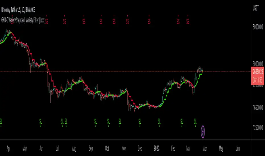
GKD-V Hurst Exponent [Loxx]Giga Kaleidoscope GKD-V Hurst Exponent is a Volatility/Volume module included in Loxx's "Giga Kaleidoscope Modularized Trading System".
█ Giga Kaleidoscope Modularized Trading System
What is Loxx's "Giga Kaleidoscope Modularized Trading System"?
The Giga Kaleidoscope Modularized Trading System is a trading system built on the philosophy of the NNFX (No Nonsense Forex) algorithmic trading.
What is the NNFX algorithmic trading strategy?
The NNFX (No-Nonsense Forex) trading system is a comprehensive approach to Forex trading that is designed to simplify the process and remove the confusion and complexity that often surrounds trading. The system was developed by a Forex trader who goes by the pseudonym "VP" and has gained a significant following in the Forex community.
The NNFX trading system is based on a set of rules and guidelines that help traders make objective and informed decisions. These rules cover all aspects of trading, including market analysis, trade entry, stop loss placement, and trade management.
Here are the main components of the NNFX trading system:
1. Trading Philosophy: The NNFX trading system is based on the idea that successful trading requires a comprehensive understanding of the market, objective analysis, and strict risk management. The system aims to remove subjective elements from trading and focuses on objective rules and guidelines.
2. Technical Analysis: The NNFX trading system relies heavily on technical analysis and uses a range of indicators to identify high-probability trading opportunities. The system uses a combination of trend-following and mean-reverting strategies to identify trades.
3. Market Structure: The NNFX trading system emphasizes the importance of understanding the market structure, including price action, support and resistance levels, and market cycles. The system uses a range of tools to identify the market structure, including trend lines, channels, and moving averages.
4. Trade Entry: The NNFX trading system has strict rules for trade entry. The system uses a combination of technical indicators to identify high-probability trades, and traders must meet specific criteria to enter a trade.
5. Stop Loss Placement: The NNFX trading system places a significant emphasis on risk management and requires traders to place a stop loss order on every trade. The system uses a combination of technical analysis and market structure to determine the appropriate stop loss level.
6. Trade Management: The NNFX trading system has specific rules for managing open trades. The system aims to minimize risk and maximize profit by using a combination of trailing stops, take profit levels, and position sizing.
Overall, the NNFX trading system is designed to be a straightforward and easy-to-follow approach to Forex trading that can be applied by traders of all skill levels.
Core components of an NNFX algorithmic trading strategy
The NNFX algorithm is built on the principles of trend, momentum, and volatility. There are six core components in the NNFX trading algorithm:
1. Volatility - price volatility; e.g., Average True Range, True Range Double, Close-to-Close, etc.
2. Baseline - a moving average to identify price trend
3. Confirmation 1 - a technical indicator used to identify trends
4. Confirmation 2 - a technical indicator used to identify trends
5. Continuation - a technical indicator used to identify trends
6. Volatility/Volume - a technical indicator used to identify volatility/volume breakouts/breakdown
7. Exit - a technical indicator used to determine when a trend is exhausted
What is Volatility in the NNFX trading system?
In the NNFX (No Nonsense Forex) trading system, ATR (Average True Range) is typically used to measure the volatility of an asset. It is used as a part of the system to help determine the appropriate stop loss and take profit levels for a trade. ATR is calculated by taking the average of the true range values over a specified period.
True range is calculated as the maximum of the following values:
-Current high minus the current low
-Absolute value of the current high minus the previous close
-Absolute value of the current low minus the previous close
ATR is a dynamic indicator that changes with changes in volatility. As volatility increases, the value of ATR increases, and as volatility decreases, the value of ATR decreases. By using ATR in NNFX system, traders can adjust their stop loss and take profit levels according to the volatility of the asset being traded. This helps to ensure that the trade is given enough room to move, while also minimizing potential losses.
Other types of volatility include True Range Double (TRD), Close-to-Close, and Garman-Klass
What is a Baseline indicator?
The baseline is essentially a moving average, and is used to determine the overall direction of the market.
The baseline in the NNFX system is used to filter out trades that are not in line with the long-term trend of the market. The baseline is plotted on the chart along with other indicators, such as the Moving Average (MA), the Relative Strength Index (RSI), and the Average True Range (ATR).
Trades are only taken when the price is in the same direction as the baseline. For example, if the baseline is sloping upwards, only long trades are taken, and if the baseline is sloping downwards, only short trades are taken. This approach helps to ensure that trades are in line with the overall trend of the market, and reduces the risk of entering trades that are likely to fail.
By using a baseline in the NNFX system, traders can have a clear reference point for determining the overall trend of the market, and can make more informed trading decisions. The baseline helps to filter out noise and false signals, and ensures that trades are taken in the direction of the long-term trend.
What is a Confirmation indicator?
Confirmation indicators are technical indicators that are used to confirm the signals generated by primary indicators. Primary indicators are the core indicators used in the NNFX system, such as the Average True Range (ATR), the Moving Average (MA), and the Relative Strength Index (RSI).
The purpose of the confirmation indicators is to reduce false signals and improve the accuracy of the trading system. They are designed to confirm the signals generated by the primary indicators by providing additional information about the strength and direction of the trend.
Some examples of confirmation indicators that may be used in the NNFX system include the Bollinger Bands, the MACD (Moving Average Convergence Divergence), and the Stochastic Oscillator. These indicators can provide information about the volatility, momentum, and trend strength of the market, and can be used to confirm the signals generated by the primary indicators.
In the NNFX system, confirmation indicators are used in combination with primary indicators and other filters to create a trading system that is robust and reliable. By using multiple indicators to confirm trading signals, the system aims to reduce the risk of false signals and improve the overall profitability of the trades.
What is a Continuation indicator?
In the NNFX (No Nonsense Forex) trading system, a continuation indicator is a technical indicator that is used to confirm a current trend and predict that the trend is likely to continue in the same direction. A continuation indicator is typically used in conjunction with other indicators in the system, such as a baseline indicator, to provide a comprehensive trading strategy.
What is a Volatility/Volume indicator?
Volume indicators, such as the On Balance Volume (OBV), the Chaikin Money Flow (CMF), or the Volume Price Trend (VPT), are used to measure the amount of buying and selling activity in a market. They are based on the trading volume of the market, and can provide information about the strength of the trend. In the NNFX system, volume indicators are used to confirm trading signals generated by the Moving Average and the Relative Strength Index. Volatility indicators include Average Direction Index, Waddah Attar, and Volatility Ratio. In the NNFX trading system, volatility is a proxy for volume and vice versa.
By using volume indicators as confirmation tools, the NNFX trading system aims to reduce the risk of false signals and improve the overall profitability of trades. These indicators can provide additional information about the market that is not captured by the primary indicators, and can help traders to make more informed trading decisions. In addition, volume indicators can be used to identify potential changes in market trends and to confirm the strength of price movements.
What is an Exit indicator?
The exit indicator is used in conjunction with other indicators in the system, such as the Moving Average (MA), the Relative Strength Index (RSI), and the Average True Range (ATR), to provide a comprehensive trading strategy.
The exit indicator in the NNFX system can be any technical indicator that is deemed effective at identifying optimal exit points. Examples of exit indicators that are commonly used include the Parabolic SAR, the Average Directional Index (ADX), and the Chandelier Exit.
The purpose of the exit indicator is to identify when a trend is likely to reverse or when the market conditions have changed, signaling the need to exit a trade. By using an exit indicator, traders can manage their risk and prevent significant losses.
In the NNFX system, the exit indicator is used in conjunction with a stop loss and a take profit order to maximize profits and minimize losses. The stop loss order is used to limit the amount of loss that can be incurred if the trade goes against the trader, while the take profit order is used to lock in profits when the trade is moving in the trader's favor.
Overall, the use of an exit indicator in the NNFX trading system is an important component of a comprehensive trading strategy. It allows traders to manage their risk effectively and improve the profitability of their trades by exiting at the right time.
How does Loxx's GKD (Giga Kaleidoscope Modularized Trading System) implement the NNFX algorithm outlined above?
Loxx's GKD v1.0 system has five types of modules (indicators/strategies). These modules are:
1. GKD-BT - Backtesting module (Volatility, Number 1 in the NNFX algorithm)
2. GKD-B - Baseline module (Baseline and Volatility/Volume, Numbers 1 and 2 in the NNFX algorithm)
3. GKD-C - Confirmation 1/2 and Continuation module (Confirmation 1/2 and Continuation, Numbers 3, 4, and 5 in the NNFX algorithm)
4. GKD-V - Volatility/Volume module (Confirmation 1/2, Number 6 in the NNFX algorithm)
5. GKD-E - Exit module (Exit, Number 7 in the NNFX algorithm)
(additional module types will added in future releases)
Each module interacts with every module by passing data between modules. Data is passed between each module as described below:
GKD-B => GKD-V => GKD-C(1) => GKD-C(2) => GKD-C(Continuation) => GKD-E => GKD-BT
That is, the Baseline indicator passes its data to Volatility/Volume. The Volatility/Volume indicator passes its values to the Confirmation 1 indicator. The Confirmation 1 indicator passes its values to the Confirmation 2 indicator. The Confirmation 2 indicator passes its values to the Continuation indicator. The Continuation indicator passes its values to the Exit indicator, and finally, the Exit indicator passes its values to the Backtest strategy.
This chaining of indicators requires that each module conform to Loxx's GKD protocol, therefore allowing for the testing of every possible combination of technical indicators that make up the six components of the NNFX algorithm.
What does the application of the GKD trading system look like?
Example trading system:
Backtest: Strategy with 1-3 take profits, trailing stop loss, multiple types of PnL volatility, and 2 backtesting styles
Baseline: Hull Moving Average
Volatility/Volume: Hurst Exponent as shown on the chart above
Confirmation 1: Vortex
Confirmation 2: Williams Percent Range
Continuation: Fisher Transform
Exit: Rex Oscillator
Each GKD indicator is denoted with a module identifier of either: GKD-BT, GKD-B, GKD-C, GKD-V, or GKD-E. This allows traders to understand to which module each indicator belongs and where each indicator fits into the GKD protocol chain.
Giga Kaleidoscope Modularized Trading System Signals (based on the NNFX algorithm)
Standard Entry
1. GKD-C Confirmation 1 Signal
2. GKD-B Baseline agrees
3. Price is within a range of 0.2x Volatility and 1.0x Volatility of the Goldie Locks Mean
4. GKD-C Confirmation 2 agrees
5. GKD-V Volatility/Volume agrees
Baseline Entry
1. GKD-B Baseline signal
2. GKD-C Confirmation 1 agrees
3. Price is within a range of 0.2x Volatility and 1.0x Volatility of the Goldie Locks Mean
4. GKD-C Confirmation 2 agrees
5. GKD-V Volatility/Volume agrees
6. GKD-C Confirmation 1 signal was less than 7 candles prior
Continuation Entry
1. Standard Entry, Baseline Entry, or Pullback; entry triggered previously
2. GKD-B Baseline hasn't crossed since entry signal trigger
3. GKD-C Confirmation Continuation Indicator signals
4. GKD-C Confirmation 1 agrees
5. GKD-B Baseline agrees
6. GKD-C Confirmation 2 agrees
1-Candle Rule Standard Entry
1. GKD-C Confirmation 1 signal
2. GKD-B Baseline agrees
3. Price is within a range of 0.2x Volatility and 1.0x Volatility of the Goldie Locks Mean
Next Candle:
1. Price retraced (Long: close < close or Short: close > close )
2. GKD-B Baseline agrees
3. GKD-C Confirmation 1 agrees
4. GKD-C Confirmation 2 agrees
5. GKD-V Volatility/Volume agrees
1-Candle Rule Baseline Entry
1. GKD-B Baseline signal
2. GKD-C Confirmation 1 agrees
3. Price is within a range of 0.2x Volatility and 1.0x Volatility of the Goldie Locks Mean
4. GKD-C Confirmation 1 signal was less than 7 candles prior
Next Candle:
1. Price retraced (Long: close < close or Short: close > close )
2. GKD-B Baseline agrees
3. GKD-C Confirmation 1 agrees
4. GKD-C Confirmation 2 agrees
5. GKD-V Volatility/Volume Agrees
PullBack Entry
1. GKD-B Baseline signal
2. GKD-C Confirmation 1 agrees
3. Price is beyond 1.0x Volatility of Baseline
Next Candle:
1. Price is within a range of 0.2x Volatility and 1.0x Volatility of the Goldie Locks Mean
3. GKD-C Confirmation 1 agrees
4. GKD-C Confirmation 2 agrees
5. GKD-V Volatility/Volume Agrees
█ GKD-C Hurst Exponent
What is the Fractal Dimension Index?
The goal of the fractal dimension index is to determine whether the market is trending or in a trading range. It does not measure the direction of the trend. A value less than 1.5 indicates that the price series is persistent or that the market is trending. Lower values of the FDI indicate a stronger trend. A value greater than 1.5 indicates that the market is in a trading range and is acting in a more random fashion.
What is the Hurst Exponent?
The Hurst exponent is a statistical measure that describes the degree of long-term memory in a time series data, including forex trading data. It is used to identify the persistence or anti-persistence of the data over different time horizons.
In forex trading, the Hurst exponent can be used to identify the degree of trendiness in price movements. When the Hurst exponent is above 0.5, it indicates that the price movements have a persistent or trending behavior, while a Hurst exponent below 0.5 suggests that the price movements are anti-persistent or mean-reverting in nature.
The Fractal Dimension Index (FDI) is another technical indicator used in forex trading that is related to the Hurst exponent. The FDI measures the degree of self-similarity or fractal dimension of the price movements over different time horizons. A high FDI indicates that the price movements are more self-similar and fractal-like, while a low FDI suggests that the price movements are less self-similar and more random in nature.
The Hurst exponent and the FDI are related because they both measure the degree of persistence or anti-persistence in price movements. In fact, the Hurst exponent can be calculated from the FDI using a simple formula. The formula relates the Hurst exponent to the FDI through the expression H = 2 - FDI.
Traders can use the Hurst exponent and the FDI in conjunction with other technical indicators to identify trading opportunities in the forex market. For example, a trader may use a high Hurst exponent or a high FDI to identify a strong trend and use a trend-following strategy. Conversely, a low Hurst exponent or a low FDI may suggest a potential trend reversal, prompting the trader to use a mean-reversion strategy.
In summary, the Hurst exponent and the FDI are two technical indicators that measure the degree of persistence or anti-persistence in price movements in the forex market. They are related because they both measure the fractal-like behavior of the price movements over different time horizons. Traders can use these indicators in combination with other technical analysis techniques to identify trading opportunities and manage risk.
Requirements
Inputs
Chained: GKD-B Baseline
Solo: NA, no inputs
Outputs
Chained: GKD-C indicators Confirmation 1 or Solo Confirmation Complex
Solo: GKD-BT Backtest
Additional features will be added in future releases.
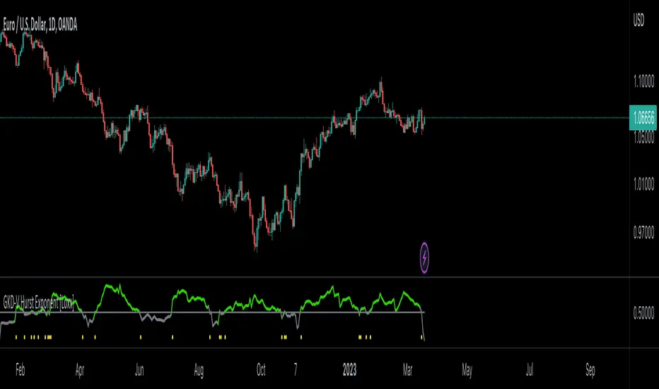
mentfx Triple MThis indicator colors the wick of a candle on any timeframe based on whether the following rules are met:
A colored wick below a candle indicates that the candles low was lower than the previous candles low, and the body of the candle closed above the previous candles low.
A colored wick above a candle indicates that the candles high was higher than the previous candles high, and the body of the candle closed below the previous candles high.
The idea behind this indicator is to fractally see a distribution (colored wick above a candle) or an accumulation (colored wick below a candle) as a confirmation once you have established a directional trend or turning point. This indicator will color any wick that meets these conditions. This indicator is meant more so as an entry confirmation, coupling it with your understanding of turning points, or likely points that price will continue in a direction - this can provide a nice confirmation.

GKD-B Baseline [Loxx]Giga Kaleidoscope Baseline is a Baseline module included in Loxx's "Giga Kaleidoscope Modularized Trading System".
What is Loxx's "Giga Kaleidoscope Modularized Trading System"?
The Giga Kaleidoscope Modularized Trading System is a trading system built on the philosophy of the NNFX (No Nonsense Forex) algorithmic trading.
What is an NNFX algorithmic trading strategy?
The NNFX algorithm is built on the principles of trend, momentum, and volatility. There are six core components in the NNFX trading algorithm:
1. Volatility - price volatility; e.g., Average True Range, True Range Double, Close-to-Close, etc.
2. Baseline - a moving average to identify price trend (such as "Baseline" shown on the chart above)
3. Confirmation 1 - a technical indicator used to identify trend. This should agree with the "Baseline"
4. Confirmation 2 - a technical indicator used to identify trend. This filters/verifies the trend identified by "Baseline" and "Confirmation 1"
5. Volatility/Volume - a technical indicator used to identify volatility/volume breakouts/breakdown.
6. Exit - a technical indicator used to determine when trend is exhausted.
How does Loxx's GKD (Giga Kaleidoscope Modularized Trading System) implement the NNFX algorithm outlined above?
Loxx's GKD v1.0 system has five types of modules (indicators/strategies). These modules are:
1. GKD-BT - Backtesting module (Volatility, Number 1 in the NNFX algorithm)
2. GKD-B - Baseline module (Baseline and Volatility/Volume, Numbers 1 and 2 in the NNFX algorithm)
3. GKD-C - Confirmation 1/2 module (Confirmation 1/2, Numbers 3 and 4 in the NNFX algorithm)
4. GKD-V - Volatility/Volume module (Confirmation 1/2, Number 5 in the NNFX algorithm)
5. GKD-E - Exit module (Exit, Number 6 in the NNFX algorithm)
(additional module types will added in future releases)
Each module interacts with every module by passing data between modules. Data is passed between each module as described below:
GKD-B => GKD-V => GKD-C(1) => GKD-C(2) => GKD-E => GKD-BT
That is, the Baseline indicator passes its data to Volatility/Volume. The Volatility/Volume indicator passes its values to the Confirmation 1 indicator. The Confirmation 1 indicator passes its values to the Confirmation 2 indicator. The Confirmation 2 indicator passes its values to the Exit indicator, and finally, the Exit indicator passes its values to the Backtest strategy.
This chaining of indicators requires that each module conform to Loxx's GKD protocol, therefore allowing for the testing of every possible combination of technical indicators that make up the six components of the NNFX algorithm.
What does the application of the GKD trading system look like?
Example trading system:
Backtest: Strategy with 1-3 take profits, trailing stop loss, multiple types of PnL volatility, and 2 backtesting styles
Baseline: Hull Moving Average as shown on the chart above
Volatility/Volume: Jurik Volty
Confirmation 1: Vortex
Confirmation 2: Fisher Transform
Exit: Rex Oscillator
Each GKD indicator is denoted with a module identifier of either: GKD-BT, GKD-B, GKD-C, GKD-V, or GKD-E. This allows traders understand to which module each indicator belongs and where each indicator fits into the GKD protocol chain.
Now that you have a general understanding of the NNFX algorithm and the GKD trading system. let's go over what's inside the GKD-B Baseline itself.
GKD Baseline Special Features and Notable Inputs
GKD Baseline v1.0 includes 63 different moving averages:
Adaptive Moving Average - AMA
ADXvma - Average Directional Volatility Moving Average
Ahrens Moving Average
Alexander Moving Average - ALXMA
Deviation Scaled Moving Average - DSMA
Donchian
Double Exponential Moving Average - DEMA
Double Smoothed Exponential Moving Average - DSEMA
Double Smoothed FEMA - DSFEMA
Double Smoothed Range Weighted EMA - DSRWEMA
Double Smoothed Wilders EMA - DSWEMA
Double Weighted Moving Average - DWMA
Ehlers Optimal Tracking Filter - EOTF
Exponential Moving Average - EMA
Fast Exponential Moving Average - FEMA
Fractal Adaptive Moving Average - FRAMA
Generalized DEMA - GDEMA
Generalized Double DEMA - GDDEMA
Hull Moving Average (Type 1) - HMA1
Hull Moving Average (Type 2) - HMA2
Hull Moving Average (Type 3) - HMA3
Hull Moving Average (Type 4) - HMA4
IE /2 - Early T3 by Tim Tilson
Integral of Linear Regression Slope - ILRS
Instantaneous Trendline
Kalman Filter
Kaufman Adaptive Moving Average - KAMA
Laguerre Filter
Leader Exponential Moving Average
Linear Regression Value - LSMA ( Least Squares Moving Average )
Linear Weighted Moving Average - LWMA
McGinley Dynamic
McNicholl EMA
Non-Lag Moving Average
Ocean NMA Moving Average - ONMAMA
Parabolic Weighted Moving Average
Probability Density Function Moving Average - PDFMA
Quadratic Regression Moving Average - QRMA
Regularized EMA - REMA
Range Weighted EMA - RWEMA
Recursive Moving Trendline
Simple Decycler - SDEC
Simple Jurik Moving Average - SJMA
Simple Moving Average - SMA
Sine Weighted Moving Average
Smoothed LWMA - SLWMA
Smoothed Moving Average - SMMA
Smoother
Super Smoother
T3
Three-pole Ehlers Butterworth
Three-pole Ehlers Smoother
Triangular Moving Average - TMA
Triple Exponential Moving Average - TEMA
Two-pole Ehlers Butterworth
Two-pole Ehlers smoother
Variable Index Dynamic Average - VIDYA
Variable Moving Average - VMA
Volume Weighted EMA - VEMA
Volume Weighted Moving Average - VWMA
Zero-Lag DEMA - Zero Lag Exponential Moving Average
Zero-Lag Moving Average
Zero Lag TEMA - Zero Lag Triple Exponential Moving Average
Adaptive Moving Average - AMA
Description. The Adaptive Moving Average (AMA) is a moving average that changes its sensitivity to price moves depending on the calculated volatility. It becomes more sensitive during periods when the price is moving smoothly in a certain direction and becomes less sensitive when the price is volatile.
ADXvma - Average Directional Volatility Moving Average
Linnsoft's ADXvma formula is a volatility-based moving average, with the volatility being determined by the value of the ADX indicator.
The ADXvma has the SMA in Chande's CMO replaced with an EMA , it then uses a few more layers of EMA smoothing before the "Volatility Index" is calculated.
A side effect is, those additional layers slow down the ADXvma when you compare it to Chande's Variable Index Dynamic Average VIDYA .
The ADXVMA provides support during uptrends and resistance during downtrends and will stay flat for longer, but will create some of the most accurate market signals when it decides to move.
Ahrens Moving Average
Richard D. Ahrens's Moving Average promises "Smoother Data" that isn't influenced by the occasional price spike. It works by using the Open and the Close in his formula so that the only time the Ahrens Moving Average will change is when the candlestick is either making new highs or new lows.
Alexander Moving Average - ALXMA
This Moving Average uses an elaborate smoothing formula and utilizes a 7 period Moving Average. It corresponds to fitting a second-order polynomial to seven consecutive observations. This moving average is rarely used in trading but is interesting as this Moving Average has been applied to diffusion indexes that tend to be very volatile.
Deviation Scaled Moving Average - DSMA
The Deviation-Scaled Moving Average is a data smoothing technique that acts like an exponential moving average with a dynamic smoothing coefficient. The smoothing coefficient is automatically updated based on the magnitude of price changes. In the Deviation-Scaled Moving Average, the standard deviation from the mean is chosen to be the measure of this magnitude. The resulting indicator provides substantial smoothing of the data even when price changes are small while quickly adapting to these changes.
Donchian
Donchian Channels are three lines generated by moving average calculations that comprise an indicator formed by upper and lower bands around a midrange or median band. The upper band marks the highest price of a security over N periods while the lower band marks the lowest price of a security over N periods.
Double Exponential Moving Average - DEMA
The Double Exponential Moving Average ( DEMA ) combines a smoothed EMA and a single EMA to provide a low-lag indicator. It's primary purpose is to reduce the amount of "lagging entry" opportunities, and like all Moving Averages, the DEMA confirms uptrends whenever price crosses on top of it and closes above it, and confirms downtrends when the price crosses under it and closes below it - but with significantly less lag.
Double Smoothed Exponential Moving Average - DSEMA
The Double Smoothed Exponential Moving Average is a lot less laggy compared to a traditional EMA . It's also considered a leading indicator compared to the EMA , and is best utilized whenever smoothness and speed of reaction to market changes are required.
Double Smoothed FEMA - DSFEMA
Same as the Double Exponential Moving Average (DEMA), but uses a faster version of EMA for its calculation.
Double Smoothed Range Weighted EMA - DSRWEMA
Range weighted exponential moving average (EMA) is, unlike the "regular" range weighted average calculated in a different way. Even though the basis - the range weighting - is the same, the way how it is calculated is completely different. By definition this type of EMA is calculated as a ratio of EMA of price*weight / EMA of weight. And the results are very different and the two should be considered as completely different types of averages. The higher than EMA to price changes responsiveness when the ranges increase remains in this EMA too and in those cases this EMA is clearly leading the "regular" EMA. This version includes double smoothing.
Double Smoothed Wilders EMA - DSWEMA
Welles Wilder was frequently using one "special" case of EMA (Exponential Moving Average) that is due to that fact (that he used it) sometimes called Wilder's EMA. This version is adding double smoothing to Wilder's EMA in order to make it "faster" (it is more responsive to market prices than the original) and is still keeping very smooth values.
Double Weighted Moving Average - DWMA
Double weighted moving average is an LWMA (Linear Weighted Moving Average). Instead of doing one cycle for calculating the LWMA, the indicator is made to cycle the loop 2 times. That produces a smoother values than the original LWMA
Ehlers Optimal Tracking Filter - EOTF
The Elher's Optimum Tracking Filter quickly adjusts rapid shifts in the price and yet is relatively smooth when the price has a sideways action. The operation of this filter is similar to Kaufman’s Adaptive Moving
Average
Exponential Moving Average - EMA
The EMA places more significance on recent data points and moves closer to price than the SMA ( Simple Moving Average ). It reacts faster to volatility due to its emphasis on recent data and is known for its ability to give greater weight to recent and more relevant data. The EMA is therefore seen as an enhancement over the SMA .
Fast Exponential Moving Average - FEMA
An Exponential Moving Average with a short look-back period.
Fractal Adaptive Moving Average - FRAMA
The Fractal Adaptive Moving Average by John Ehlers is an intelligent adaptive Moving Average which takes the importance of price changes into account and follows price closely enough to display significant moves whilst remaining flat if price ranges. The FRAMA does this by dynamically adjusting the look-back period based on the market's fractal geometry.
Generalized DEMA - GDEMA
The double exponential moving average (DEMA), was developed by Patrick Mulloy in an attempt to reduce the amount of lag time found in traditional moving averages. It was first introduced in the February 1994 issue of the magazine Technical Analysis of Stocks & Commodities in Mulloy's article "Smoothing Data with Faster Moving Averages.". Instead of using fixed multiplication factor in the final DEMA formula, the generalized version allows you to change it. By varying the "volume factor" form 0 to 1 you apply different multiplications and thus producing DEMA with different "speed" - the higher the volume factor is the "faster" the DEMA will be (but also the slope of it will be less smooth). The volume factor is limited in the calculation to 1 since any volume factor that is larger than 1 is increasing the overshooting to the extent that some volume factors usage makes the indicator unusable.
Generalized Double DEMA - GDDEMA
The double exponential moving average (DEMA), was developed by Patrick Mulloy in an attempt to reduce the amount of lag time found in traditional moving averages. It was first introduced in the February 1994 issue of the magazine Technical Analysis of Stocks & Commodities in Mulloy's article "Smoothing Data with Faster Moving Averages''. This is an extension of the Generalized DEMA using Tim Tillsons (the inventor of T3) idea, and is using GDEMA of GDEMA for calculation (which is the "middle step" of T3 calculation). Since there are no versions showing that middle step, this version covers that too. The result is smoother than Generalized DEMA, but is less smooth than T3 - one has to do some experimenting in order to find the optimal way to use it, but in any case, since it is "faster" than the T3 (Tim Tillson T3) and still smooth, it looks like a good compromise between speed and smoothness.
Hull Moving Average (Type 1) - HMA1
Alan Hull's HMA makes use of weighted moving averages to prioritize recent values and greatly reduce lag whilst maintaining the smoothness of a traditional Moving Average. For this reason, it's seen as a well-suited Moving Average for identifying entry points. This version uses SMA for smoothing.
Hull Moving Average (Type 2) - HMA2
Alan Hull's HMA makes use of weighted moving averages to prioritize recent values and greatly reduce lag whilst maintaining the smoothness of a traditional Moving Average. For this reason, it's seen as a well-suited Moving Average for identifying entry points. This version uses EMA for smoothing.
Hull Moving Average (Type 3) - HMA3
Alan Hull's HMA makes use of weighted moving averages to prioritize recent values and greatly reduce lag whilst maintaining the smoothness of a traditional Moving Average. For this reason, it's seen as a well-suited Moving Average for identifying entry points. This version uses LWMA for smoothing.
Hull Moving Average (Type 4) - HMA4
Alan Hull's HMA makes use of weighted moving averages to prioritize recent values and greatly reduce lag whilst maintaining the smoothness of a traditional Moving Average. For this reason, it's seen as a well-suited Moving Average for identifying entry points. This version uses SMMA for smoothing.
IE /2 - Early T3 by Tim Tilson and T3 new
T3 is basically an EMA on steroids, You can read about T3 here:
Integral of Linear Regression Slope - ILRS
A Moving Average where the slope of a linear regression line is simply integrated as it is fitted in a moving window of length N (natural numbers in maths) across the data. The derivative of ILRS is the linear regression slope. ILRS is not the same as a SMA ( Simple Moving Average ) of length N, which is actually the midpoint of the linear regression line as it moves across the data.
Instantaneous Trendline
The Instantaneous Trendline is created by removing the dominant cycle component from the price information which makes this Moving Average suitable for medium to long-term trading.
Kalman Filter
Kalman filter is an algorithm that uses a series of measurements observed over time, containing statistical noise and other inaccuracies. This means that the filter was originally designed to work with noisy data. Also, it is able to work with incomplete data. Another advantage is that it is designed for and applied in dynamic systems; our price chart belongs to such systems. This version is true to the original design of the trade-ready Kalman Filter where velocity is the triggering mechanism.
Kalman Filter is a more accurate smoothing/prediction algorithm than the moving average because it is adaptive: it accounts for estimation errors and tries to adjust its predictions from the information it learned in the previous stage. Theoretically, Kalman Filter consists of measurement and transition components.
Kaufman Adaptive Moving Average - KAMA
Developed by Perry Kaufman, Kaufman's Adaptive Moving Average (KAMA) is a moving average designed to account for market noise or volatility. KAMA will closely follow prices when the price swings are relatively small and the noise is low.
Laguerre Filter
The Laguerre Filter is a smoothing filter which is based on Laguerre polynomials. The filter requires the current price, three prior prices, a user defined factor called Alpha to fill its calculation.
Adjusting the Alpha coefficient is used to increase or decrease its lag and its smoothness.
Leader Exponential Moving Average
The Leader EMA was created by Giorgos E. Siligardos who created a Moving Average which was able to eliminate lag altogether whilst maintaining some smoothness. It was first described during his research paper "MACD Leader" where he applied this to the MACD to improve its signals and remove its lagging issue. This filter uses his leading MACD's "modified EMA" and can be used as a zero lag filter.
Linear Regression Value - LSMA ( Least Squares Moving Average )
LSMA as a Moving Average is based on plotting the end point of the linear regression line. It compares the current value to the prior value and a determination is made of a possible trend, eg. the linear regression line is pointing up or down.
Linear Weighted Moving Average - LWMA
LWMA reacts to price quicker than the SMA and EMA . Although it's similar to the Simple Moving Average , the difference is that a weight coefficient is multiplied to the price which means the most recent price has the highest weighting, and each prior price has progressively less weight. The weights drop in a linear fashion.
McGinley Dynamic
John McGinley created this Moving Average to track prices better than traditional Moving Averages. It does this by incorporating an automatic adjustment factor into its formula, which speeds (or slows) the indicator in trending, or ranging, markets.
McNicholl EMA
Dennis McNicholl developed this Moving Average to use as his center line for his "Better Bollinger Bands" indicator and was successful because it responded better to volatility changes over the standard SMA and managed to avoid common whipsaws.
Non-lag moving average
The Non Lag Moving average follows price closely and gives very quick signals as well as early signals of price change. As a standalone Moving Average, it should not be used on its own, but as an additional confluence tool for early signals.
Ocean NMA Moving Average - ONMAMA
Created by Jim Sloman, the NMA is a moving average that automatically adjusts to volatility without being programmed to do so. For more info, read his guide "Ocean Theory, an Introduction"
Parabolic Weighted Moving Average
The Parabolic Weighted Moving Average is a variation of the Linear Weighted Moving Average . The Linear Weighted Moving Average calculates the average by assigning different weights to each element in its calculation. The Parabolic Weighted Moving Average is a variation that allows weights to be changed to form a parabolic curve. It is done simply by using the Power parameter of this indicator.
Probability Density Function Moving Average - PDFMA
Probability density function based MA is a sort of weighted moving average that uses probability density function to calculate the weights. By its nature it is similar to a lot of digital filters.
Quadratic Regression Moving Average - QRMA
A quadratic regression is the process of finding the equation of the parabola that best fits a set of data. This moving average is an obscure concept that was posted to Forex forums in around 2008.
Regularized EMA - REMA
The regularized exponential moving average (REMA) by Chris Satchwell is a variation on the EMA (see Exponential Moving Average) designed to be smoother but not introduce too much extra lag.
Range Weighted EMA - RWEMA
This indicator is a variation of the range weighted EMA. The variation comes from a possible need to make that indicator a bit less "noisy" when it comes to slope changes. The method used for calculating this variation is the method described by Lee Leibfarth in his article "Trading With An Adaptive Price Zone".
Recursive Moving Trendline
Dennis Meyers's Recursive Moving Trendline uses a recursive (repeated application of a rule) polynomial fit, a technique that uses a small number of past values estimations of price and today's price to predict tomorrow's price.
Simple Decycler - SDEC
The Ehlers Simple Decycler study is a virtually zero-lag technical indicator proposed by John F. Ehlers. The original idea behind this study (and several others created by John F. Ehlers) is that market data can be considered a continuum of cycle periods with different cycle amplitudes. Thus, trending periods can be considered segments of longer cycles, or, in other words, low-frequency segments. Applying the right filter might help identify these segments.
Simple Loxx Moving Average - SLMA
A three stage moving average combining an adaptive EMA, a Kalman Filter, and a Kauffman adaptive filter.
Simple Moving Average - SMA
The SMA calculates the average of a range of prices by adding recent prices and then dividing that figure by the number of time periods in the calculation average. It is the most basic Moving Average which is seen as a reliable tool for starting off with Moving Average studies. As reliable as it may be, the basic moving average will work better when it's enhanced into an EMA .
Sine Weighted Moving Average
The Sine Weighted Moving Average assigns the most weight at the middle of the data set. It does this by weighting from the first half of a Sine Wave Cycle and the most weighting is given to the data in the middle of that data set. The Sine WMA closely resembles the TMA (Triangular Moving Average).
Smoothed LWMA - SLWMA
A smoothed version of the LWMA
Smoothed Moving Average - SMMA
The Smoothed Moving Average is similar to the Simple Moving Average ( SMA ), but aims to reduce noise rather than reduce lag. SMMA takes all prices into account and uses a long lookback period. Due to this, it's seen as an accurate yet laggy Moving Average.
Smoother
The Smoother filter is a faster-reacting smoothing technique which generates considerably less lag than the SMMA ( Smoothed Moving Average ). It gives earlier signals but can also create false signals due to its earlier reactions. This filter is sometimes wrongly mistaken for the superior Jurik Smoothing algorithm.
Super Smoother
The Super Smoother filter uses John Ehlers’s “Super Smoother” which consists of a Two pole Butterworth filter combined with a 2-bar SMA ( Simple Moving Average ) that suppresses the 22050 Hz Nyquist frequency: A characteristic of a sampler, which converts a continuous function or signal into a discrete sequence.
Three-pole Ehlers Butterworth
The 3 pole Ehlers Butterworth (as well as the Two pole Butterworth) are both superior alternatives to the EMA and SMA . They aim at producing less lag whilst maintaining accuracy. The 2 pole filter will give you a better approximation for price, whereas the 3 pole filter has superior smoothing.
Three-pole Ehlers smoother
The 3 pole Ehlers smoother works almost as close to price as the above mentioned 3 Pole Ehlers Butterworth. It acts as a strong baseline for signals but removes some noise. Side by side, it hardly differs from the Three Pole Ehlers Butterworth but when examined closely, it has better overshoot reduction compared to the 3 pole Ehlers Butterworth.
Triangular Moving Average - TMA
The TMA is similar to the EMA but uses a different weighting scheme. Exponential and weighted Moving Averages will assign weight to the most recent price data. Simple moving averages will assign the weight equally across all the price data. With a TMA (Triangular Moving Average), it is double smoother (averaged twice) so the majority of the weight is assigned to the middle portion of the data.
Triple Exponential Moving Average - TEMA
The TEMA uses multiple EMA calculations as well as subtracting lag to create a tool which can be used for scalping pullbacks. As it follows price closely, its signals are considered very noisy and should only be used in extremely fast-paced trading conditions.
Two-pole Ehlers Butterworth
The 2 pole Ehlers Butterworth (as well as the three pole Butterworth mentioned above) is another filter that cuts out the noise and follows the price closely. The 2 pole is seen as a faster, leading filter over the 3 pole and follows price a bit more closely. Analysts will utilize both a 2 pole and a 3 pole Butterworth on the same chart using the same period, but having both on chart allows its crosses to be traded.
Two-pole Ehlers smoother
A smoother version of the Two pole Ehlers Butterworth. This filter is the faster version out of the 3 pole Ehlers Butterworth. It does a decent job at cutting out market noise whilst emphasizing a closer following to price over the 3 pole Ehlers .
Variable Index Dynamic Average - VIDYA
Variable Index Dynamic Average Technical Indicator ( VIDYA ) was developed by Tushar Chande. It is an original method of calculating the Exponential Moving Average ( EMA ) with the dynamically changing period of averaging.
Variable Moving Average - VMA
The Variable Moving Average (VMA) is a study that uses an Exponential Moving Average being able to automatically adjust its smoothing factor according to the market volatility.
Volume Weighted EMA - VEMA
An EMA that uses a volume and price weighted calculation instead of the standard price input.
Volume Weighted Moving Average - VWMA
A Volume Weighted Moving Average is a moving average where more weight is given to bars with heavy volume than with light volume. Thus the value of the moving average will be closer to where most trading actually happened than it otherwise would be without being volume weighted.
Zero-Lag DEMA - Zero Lag Double Exponential Moving Average
John Ehlers's Zero Lag DEMA's aim is to eliminate the inherent lag associated with all trend following indicators which average a price over time. Because this is a Double Exponential Moving Average with Zero Lag, it has a tendency to overshoot and create a lot of false signals for swing trading. It can however be used for quick scalping or as a secondary indicator for confluence.
Zero-Lag Moving Average
The Zero Lag Moving Average is described by its creator, John Ehlers , as a Moving Average with absolutely no delay. And it's for this reason that this filter will cause a lot of abrupt signals which will not be ideal for medium to long-term traders. This filter is designed to follow price as close as possible whilst de-lagging data instead of basing it on regular data. The way this is done is by attempting to remove the cumulative effect of the Moving Average.
Zero-Lag TEMA - Zero Lag Triple Exponential Moving Average
Just like the Zero Lag DEMA , this filter will give you the fastest signals out of all the Zero Lag Moving Averages. This is useful for scalping but dangerous for medium to long-term traders, especially during market Volatility and news events. Having no lag, this filter also has no smoothing in its signals and can cause some very bizarre behavior when applied to certain indicators.
Exotic Triggers
This version of Baseline allows the user to select from exotic or source triggers. An exotic trigger determines trend by either slope or some other mechanism that is special to each moving average. A source trigger is one of 32 different source types from Loxx's Exotic Source Types. You can read about these source types here:
Volatility Goldie Locks Zone
This volatility filter is the standard first pass filter that is used for all NNFX systems despite the additional volatility/volume filter used in step 5. For this filter, price must fall into a range of maximum and minimum values calculated using multiples of volatility. Unlike the standard NNFX systems, this version of volatility filtering is separated from the core Baseline and uses it's own moving average with Loxx's Exotic Source Types. The green and red dots at the top of the chart denote whether a candle qualifies for a either or long or short respectively. The green and red triangles at the bottom of the chart denote whether the trigger has crossed up or down and qualifies inside the Goldie Locks zone. White coloring of the Goldie Locks Zone mean line is where volatility is too low to trade.
Volatility Types Included
v1.0 Included Volatility
Close-to-Close
Close-to-Close volatility is a classic and most commonly used volatility measure, sometimes referred to as historical volatility .
Volatility is an indicator of the speed of a stock price change. A stock with high volatility is one where the price changes rapidly and with a bigger amplitude. The more volatile a stock is, the riskier it is.
Close-to-close historical volatility calculated using only stock's closing prices. It is the simplest volatility estimator. But in many cases, it is not precise enough. Stock prices could jump considerably during a trading session, and return to the open value at the end. That means that a big amount of price information is not taken into account by close-to-close volatility .
Despite its drawbacks, Close-to-Close volatility is still useful in cases where the instrument doesn't have intraday prices. For example, mutual funds calculate their net asset values daily or weekly, and thus their prices are not suitable for more sophisticated volatility estimators.
Parkinson
Parkinson volatility is a volatility measure that uses the stock’s high and low price of the day.
The main difference between regular volatility and Parkinson volatility is that the latter uses high and low prices for a day, rather than only the closing price. That is useful as close to close prices could show little difference while large price movements could have happened during the day. Thus Parkinson's volatility is considered to be more precise and requires less data for calculation than the close-close volatility .
One drawback of this estimator is that it doesn't take into account price movements after market close. Hence it systematically undervalues volatility . That drawback is taken into account in the Garman-Klass's volatility estimator.
Garman-Klass
Garman Klass is a volatility estimator that incorporates open, low, high, and close prices of a security.
Garman-Klass volatility extends Parkinson's volatility by taking into account the opening and closing price. As markets are most active during the opening and closing of a trading session, it makes volatility estimation more accurate.
Garman and Klass also assumed that the process of price change is a process of continuous diffusion (Geometric Brownian motion). However, this assumption has several drawbacks. The method is not robust for opening jumps in price and trend movements.
Despite its drawbacks, the Garman-Klass estimator is still more effective than the basic formula since it takes into account not only the price at the beginning and end of the time interval but also intraday price extremums.
Researchers Rogers and Satchel have proposed a more efficient method for assessing historical volatility that takes into account price trends. See Rogers-Satchell Volatility for more detail.
Rogers-Satchell
Rogers-Satchell is an estimator for measuring the volatility of securities with an average return not equal to zero.
Unlike Parkinson and Garman-Klass estimators, Rogers-Satchell incorporates drift term (mean return not equal to zero). As a result, it provides a better volatility estimation when the underlying is trending.
The main disadvantage of this method is that it does not take into account price movements between trading sessions. It means an underestimation of volatility since price jumps periodically occur in the market precisely at the moments between sessions.
A more comprehensive estimator that also considers the gaps between sessions was developed based on the Rogers-Satchel formula in the 2000s by Yang-Zhang. See Yang Zhang Volatility for more detail.
Yang-Zhang
Yang Zhang is a historical volatility estimator that handles both opening jumps and the drift and has a minimum estimation error.
We can think of the Yang-Zhang volatility as the combination of the overnight (close-to-open volatility ) and a weighted average of the Rogers-Satchell volatility and the day’s open-to-close volatility . It considered being 14 times more efficient than the close-to-close estimator.
Garman-Klass-Yang-Zhang
Garman-Klass-Yang-Zhang (GKYZ) volatility estimator consists of using the returns of open, high, low, and closing prices in its calculation.
GKYZ volatility estimator takes into account overnight jumps but not the trend, i.e. it assumes that the underlying asset follows a GBM process with zero drift. Therefore the GKYZ volatility estimator tends to overestimate the volatility when the drift is different from zero. However, for a GBM process, this estimator is eight times more efficient than the close-to-close volatility estimator.
Exponential Weighted Moving Average
The Exponentially Weighted Moving Average (EWMA) is a quantitative or statistical measure used to model or describe a time series. The EWMA is widely used in finance, the main applications being technical analysis and volatility modeling.
The moving average is designed as such that older observations are given lower weights. The weights fall exponentially as the data point gets older – hence the name exponentially weighted.
The only decision a user of the EWMA must make is the parameter lambda. The parameter decides how important the current observation is in the calculation of the EWMA. The higher the value of lambda, the more closely the EWMA tracks the original time series.
Standard Deviation of Log Returns
This is the simplest calculation of volatility . It's the standard deviation of ln(close/close(1))
Pseudo GARCH(2,2)
This is calculated using a short- and long-run mean of variance multiplied by θ.
θavg(var ;M) + (1 − θ) avg (var ;N) = 2θvar/(M+1-(M-1)L) + 2(1-θ)var/(M+1-(M-1)L)
Solving for θ can be done by minimizing the mean squared error of estimation; that is, regressing L^-1var - avg (var; N) against avg (var; M) - avg (var; N) and using the resulting beta estimate as θ.
Average True Range
The average true range (ATR) is a technical analysis indicator, introduced by market technician J. Welles Wilder Jr. in his book New Concepts in Technical Trading Systems, that measures market volatility by decomposing the entire range of an asset price for that period.
The true range indicator is taken as the greatest of the following: current high less the current low; the absolute value of the current high less the previous close; and the absolute value of the current low less the previous close. The ATR is then a moving average, generally using 14 days, of the true ranges.
True Range Double
A special case of ATR that attempts to correct for volatility skew.
Additional features will be added in future releases.
This indicator is only available to ALGX Trading VIP group members . You can see the Author's Instructions below to get more information on how to get access.
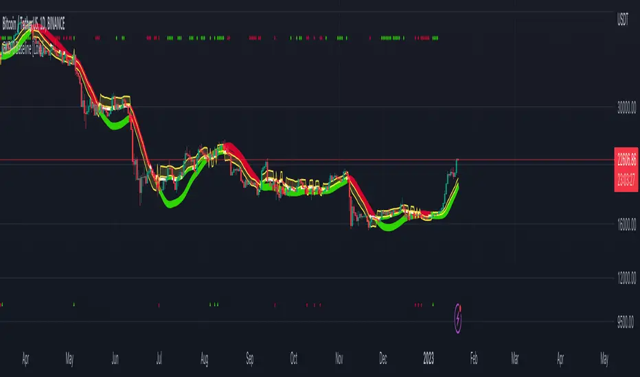
JFD-Adaptive, GKYZ-Filtered KAMA [Loxx]JFD-Adaptive, GKYZ-Filtered KAMA is a Kaufman Adaptive Moving Average with the option to make it Jurik Fractal Dimension Adaptive. This also includes a Garman-Klass-Yang-Zhang Historical Volatility Filter to reduce noise.
What is KAMA?
Developed by Perry Kaufman, Kaufman's Adaptive Moving Average ( KAMA ) is a moving average designed to account for market noise or volatility . KAMA will closely follow prices when the price swings are relatively small and the noise is low. KAMA will adjust when the price swings widen and follow prices from a greater distance. This trend-following indicator can be used to identify the overall trend, time turning points and filter price movements.
What is Jurik Fractal Dimension?
There is a weak and a strong way to measure the random quality of a time series.
The weak way is to use the random walk index ( RWI ). You can download it from the Omega web site. It makes the assumption that the market is moving randomly with an average distance D per move and proposes an amount the market should have changed over N bars of time. If the market has traveled less, then the action is considered random, otherwise it's considered trending.
The problem with this method is that taking the average distance is valid for a Normal (Gaussian) distribution of price activity. However, price action is rarely Normal, with large price jumps occuring much more frequently than a Normal distribution would expect. Consequently, big jumps throw the RWI way off, producing invalid results.
The strong way is to not make any assumption regarding the distribution of price changes and, instead, measure the fractal dimension of the time series. Fractal Dimension requires a lot of data to be accurate. If you are trading 30 minute bars, use a multi-chart where this indicator is running on 5 minute bars and you are trading on 30 minute bars.
What is Garman-Klass-Yang-Zhang Historical Volatility?
Yang and Zhang derived an extension to the Garman Klass historical volatility estimator that allows for opening jumps. It assumes Brownian motion with zero drift. This is currently the preferred version of open-high-low-close volatility estimator for zero drift and has an efficiency of 8 times the classic close-to-close estimator. Note that when the drift is nonzero, but instead relative large to the volatility , this estimator will tend to overestimate the volatility . The Garman-Klass-Yang-Zhang Historical Volatility calculation is as follows:
GKYZHV = sqrt((Z/n) * sum((log(open(k)/close( k-1 )))^2 + (0.5*(log(high(k)/low(k)))^2) - (2*log(2) - 1)*(log(close(k)/open(2:end)))^2))
Included
Alerts
Signals
Loxx's Expanded Source Types
Bar coloring
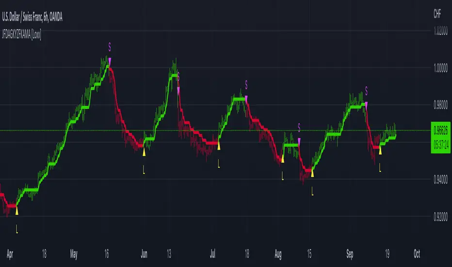
End-pointed SSA of FDASMA [Loxx]End-pointed SSA of FDASMA is a modification of Fractal-Dimension-Adaptive SMA (FDASMA) using End-Pointed Singular Spectrum Analysis. This is a multilayer adaptive indicator.
What is the Fractal Dimension Index?
The goal of the fractal dimension index is to determine whether the market is trending or in a trading range. It does not measure the direction of the trend. A value less than 1.5 indicates that the price series is persistent or that the market is trending. Lower values of the FDI indicate a stronger trend. A value greater than 1.5 indicates that the market is in a trading range and is acting in a more random fashion.
See here for more info:
Fractal-Dimension-Adaptive SMA (FDASMA) w/ DSL
What is Singular Spectrum Analysis ( SSA )?
Singular spectrum analysis ( SSA ) is a technique of time series analysis and forecasting. It combines elements of classical time series analysis, multivariate statistics, multivariate geometry, dynamical systems and signal processing. SSA aims at decomposing the original series into a sum of a small number of interpretable components such as a slowly varying trend, oscillatory components and a ‘structureless’ noise. It is based on the singular value decomposition ( SVD ) of a specific matrix constructed upon the time series. Neither a parametric model nor stationarity-type conditions have to be assumed for the time series. This makes SSA a model-free method and hence enables SSA to have a very wide range of applicability.
For our purposes here, we are only concerned with the "Caterpillar" SSA . This methodology was developed in the former Soviet Union independently (the ‘iron curtain effect’) of the mainstream SSA . The main difference between the main-stream SSA and the "Caterpillar" SSA is not in the algorithmic details but rather in the assumptions and in the emphasis in the study of SSA properties. To apply the mainstream SSA , one often needs to assume some kind of stationarity of the time series and think in terms of the "signal plus noise" model (where the noise is often assumed to be ‘red’). In the "Caterpillar" SSA , the main methodological stress is on separability (of one component of the series from another one) and neither the assumption of stationarity nor the model in the form "signal plus noise" are required.
"Caterpillar" SSA
The basic "Caterpillar" SSA algorithm for analyzing one-dimensional time series consists of:
Transformation of the one-dimensional time series to the trajectory matrix by means of a delay procedure (this gives the name to the whole technique);
Singular Value Decomposition of the trajectory matrix;
Reconstruction of the original time series based on a number of selected eigenvectors.
This decomposition initializes forecasting procedures for both the original time series and its components. The method can be naturally extended to multidimensional time series and to image processing.
The method is a powerful and useful tool of time series analysis in meteorology, hydrology, geophysics, climatology and, according to our experience, in economics, biology, physics, medicine and other sciences; that is, where short and long, one-dimensional and multidimensional, stationary and non-stationary, almost deterministic and noisy time series are to be analyzed.
Included:
Bar coloring
Alerts
Signals
Loxx's Expanded Source Types
CFB-Adaptive Trend Cipher Candles [Loxx]CFB-Adaptive Trend Cipher Candles is a candle coloring indicator that shows both trend and trend exhaustion using Composite Fractal Behavior price trend analysis. To do this, we first calculate the dynamic period outputs from the CFB algorithm and then we injection those period inputs into a correlation function that correlates price input price to the candle index. The closer the correlation is to 1, the lighter the green color until the color turns yellow, sometimes, indicating upward price exhaustion. The closer the correlation is to -1, the lighter the red color until it reaches Fuchsia color indicating downward price exhaustion. Green means uptrend, red means downtrend, yellow means reversal from uptrend to downtrend, fuchsia means reversal from downtrend to uptrend.
What is Composite Fractal Behavior ( CFB )?
All around you mechanisms adjust themselves to their environment. From simple thermostats that react to air temperature to computer chips in modern cars that respond to changes in engine temperature, r.p.m.'s, torque, and throttle position. It was only a matter of time before fast desktop computers applied the mathematics of self-adjustment to systems that trade the financial markets.
Unlike basic systems with fixed formulas, an adaptive system adjusts its own equations. For example, start with a basic channel breakout system that uses the highest closing price of the last N bars as a threshold for detecting breakouts on the up side. An adaptive and improved version of this system would adjust N according to market conditions, such as momentum, price volatility or acceleration.
Since many systems are based directly or indirectly on cycles, another useful measure of market condition is the periodic length of a price chart's dominant cycle, (DC), that cycle with the greatest influence on price action.
The utility of this new DC measure was noted by author Murray Ruggiero in the January '96 issue of Futures Magazine. In it. Mr. Ruggiero used it to adaptive adjust the value of N in a channel breakout system. He then simulated trading 15 years of D-Mark futures in order to compare its performance to a similar system that had a fixed optimal value of N. The adaptive version produced 20% more profit!
This DC index utilized the popular MESA algorithm (a formulation by John Ehlers adapted from Burg's maximum entropy algorithm, MEM). Unfortunately, the DC approach is problematic when the market has no real dominant cycle momentum, because the mathematics will produce a value whether or not one actually exists! Therefore, we developed a proprietary indicator that does not presuppose the presence of market cycles. It's called CFB (Composite Fractal Behavior) and it works well whether or not the market is cyclic.
CFB examines price action for a particular fractal pattern, categorizes them by size, and then outputs a composite fractal size index. This index is smooth, timely and accurate
Essentially, CFB reveals the length of the market's trending action time frame. Long trending activity produces a large CFB index and short choppy action produces a small index value. Investors have found many applications for CFB which involve scaling other existing technical indicators adaptively, on a bar-to-bar basis.
Included
Loxx's Expanded Source Types
Related indicators:
Adaptive Trend Cipher loxx]
Dynamic Zones Polychromatic Momentum Candles
RSI Precision Trend Candles
CFB-Adaptive, Jurik DMX Histogram [Loxx]Jurik DMX Histogram is the ultra-smooth, low lag version of your classic DMI indicator. This is a momentum indicator. You can use this indicator standalone or as part of a system with a moving average and a mean reversion indicator. This indicator has both composite fractal behavior adaptive inputs and fixed inputs. The default is CFB adaptive. Dark green means strong push up, dark red, strong push down. Light green means weak push up, and light red means weak push down.
What is the directional movement index?
The directional movement index (DMI) is an indicator developed by J. Welles Wilder in 1978 that identifies in which direction the price of an asset is moving. The indicator does this by comparing prior highs and lows and drawing two lines: a positive directional movement line ( +DI ) and a negative directional movement line ( -DI ). An optional third line, called the average directional index ( ADX ), can also be used to gauge the strength of the uptrend or downtrend.
When +DI is above -DI , there is more upward pressure than downward pressure in the price. Conversely, if -DI is above +DI , then there is more downward pressure on the price. This indicator may help traders assess the trend direction. Crossovers between the lines are also sometimes used as trade signals to buy or sell.
What is Composite Fractal Behavior ( CFB )?
All around you mechanisms adjust themselves to their environment. From simple thermostats that react to air temperature to computer chips in modern cars that respond to changes in engine temperature, r.p.m.'s, torque, and throttle position. It was only a matter of time before fast desktop computers applied the mathematics of self-adjustment to systems that trade the financial markets.
Unlike basic systems with fixed formulas, an adaptive system adjusts its own equations. For example, start with a basic channel breakout system that uses the highest closing price of the last N bars as a threshold for detecting breakouts on the up side. An adaptive and improved version of this system would adjust N according to market conditions, such as momentum, price volatility or acceleration.
Since many systems are based directly or indirectly on cycles, another useful measure of market condition is the periodic length of a price chart's dominant cycle, (DC), that cycle with the greatest influence on price action.
The utility of this new DC measure was noted by author Murray Ruggiero in the January '96 issue of Futures Magazine. In it. Mr. Ruggiero used it to adaptive adjust the value of N in a channel breakout system. He then simulated trading 15 years of D-Mark futures in order to compare its performance to a similar system that had a fixed optimal value of N. The adaptive version produced 20% more profit!
This DC index utilized the popular MESA algorithm (a formulation by John Ehlers adapted from Burg's maximum entropy algorithm, MEM). Unfortunately, the DC approach is problematic when the market has no real dominant cycle momentum, because the mathematics will produce a value whether or not one actually exists! Therefore, we developed a proprietary indicator that does not presuppose the presence of market cycles. It's called CFB (Composite Fractal Behavior) and it works well whether or not the market is cyclic.
CFB examines price action for a particular fractal pattern, categorizes them by size, and then outputs a composite fractal size index. This index is smooth, timely and accurate
Essentially, CFB reveals the length of the market's trending action time frame. Long trending activity produces a large CFB index and short choppy action produces a small index value. Investors have found many applications for CFB which involve scaling other existing technical indicators adaptively, on a bar-to-bar basis.
What is Jurik Volty used in the Juirk Filter?
One of the lesser known qualities of Juirk smoothing is that the Jurik smoothing process is adaptive. "Jurik Volty" (a sort of market volatility ) is what makes Jurik smoothing adaptive. The Jurik Volty calculation can be used as both a standalone indicator and to smooth other indicators that you wish to make adaptive.
What is the Jurik Moving Average?
Have you noticed how moving averages add some lag (delay) to your signals? ... especially when price gaps up or down in a big move, and you are waiting for your moving average to catch up? Wait no more! JMA eliminates this problem forever and gives you the best of both worlds: low lag and smooth lines.
Ideally, you would like a filtered signal to be both smooth and lag-free. Lag causes delays in your trades, and increasing lag in your indicators typically result in lower profits. In other words, late comers get what's left on the table after the feast has already begun.
Included:
Alerts
Loxx's Expanded Source Types
Signals
Bar coloring
