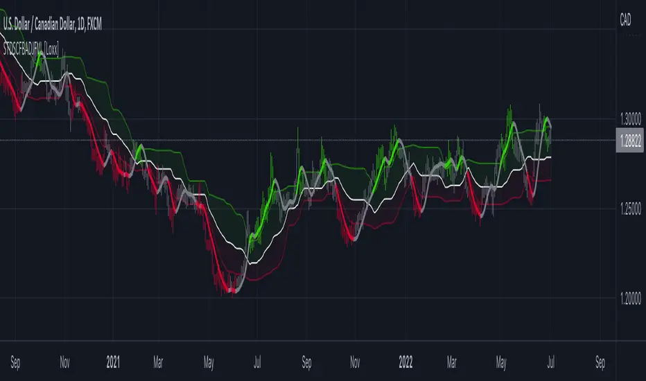
CFB-Adaptive, Williams %R w/ Dynamic Zones [Loxx]CFB-Adaptive, Williams %R w/ Dynamic Zones is a Jurik-Composite-Fractal-Behavior-Adaptive Williams % Range indicator with Dynamic Zones. These additions to the WPR calculation reduce noise and return a signal that is more viable than WPR alone.
What is Williams %R?
Williams %R , also known as the Williams Percent Range, is a type of momentum indicator that moves between 0 and -100 and measures overbought and oversold levels. The Williams %R may be used to find entry and exit points in the market. The indicator is very similar to the Stochastic oscillator and is used in the same way. It was developed by Larry Williams and it compares a stock’s closing price to the high-low range over a specific period, typically 14 days or periods.
What is Composite Fractal Behavior ( CFB )?
All around you mechanisms adjust themselves to their environment. From simple thermostats that react to air temperature to computer chips in modern cars that respond to changes in engine temperature, r.p.m.'s, torque, and throttle position. It was only a matter of time before fast desktop computers applied the mathematics of self-adjustment to systems that trade the financial markets.
Unlike basic systems with fixed formulas, an adaptive system adjusts its own equations. For example, start with a basic channel breakout system that uses the highest closing price of the last N bars as a threshold for detecting breakouts on the up side. An adaptive and improved version of this system would adjust N according to market conditions, such as momentum, price volatility or acceleration.
Since many systems are based directly or indirectly on cycles, another useful measure of market condition is the periodic length of a price chart's dominant cycle, (DC), that cycle with the greatest influence on price action.
The utility of this new DC measure was noted by author Murray Ruggiero in the January '96 issue of Futures Magazine. In it. Mr. Ruggiero used it to adaptive adjust the value of N in a channel breakout system. He then simulated trading 15 years of D-Mark futures in order to compare its performance to a similar system that had a fixed optimal value of N. The adaptive version produced 20% more profit!
This DC index utilized the popular MESA algorithm (a formulation by John Ehlers adapted from Burg's maximum entropy algorithm, MEM). Unfortunately, the DC approach is problematic when the market has no real dominant cycle momentum, because the mathematics will produce a value whether or not one actually exists! Therefore, we developed a proprietary indicator that does not presuppose the presence of market cycles. It's called CFB (Composite Fractal Behavior) and it works well whether or not the market is cyclic.
CFB examines price action for a particular fractal pattern, categorizes them by size, and then outputs a composite fractal size index. This index is smooth, timely and accurate
Essentially, CFB reveals the length of the market's trending action time frame. Long trending activity produces a large CFB index and short choppy action produces a small index value. Investors have found many applications for CFB which involve scaling other existing technical indicators adaptively, on a bar-to-bar basis.
What is Jurik Volty used in the Juirk Filter?
One of the lesser known qualities of Juirk smoothing is that the Jurik smoothing process is adaptive. "Jurik Volty" (a sort of market volatility ) is what makes Jurik smoothing adaptive. The Jurik Volty calculation can be used as both a standalone indicator and to smooth other indicators that you wish to make adaptive.
What is the Jurik Moving Average?
Have you noticed how moving averages add some lag (delay) to your signals? ... especially when price gaps up or down in a big move, and you are waiting for your moving average to catch up? Wait no more! JMA eliminates this problem forever and gives you the best of both worlds: low lag and smooth lines.
Ideally, you would like a filtered signal to be both smooth and lag-free. Lag causes delays in your trades, and increasing lag in your indicators typically result in lower profits. In other words, late comers get what's left on the table after the feast has already begun.
What are Dynamic Zones?
As explained in "Stocks & Commodities V15:7 (306-310): Dynamic Zones by Leo Zamansky, Ph .D., and David Stendahl"
Most indicators use a fixed zone for buy and sell signals. Here’ s a concept based on zones that are responsive to past levels of the indicator.
One approach to active investing employs the use of oscillators to exploit tradable market trends. This investing style follows a very simple form of logic: Enter the market only when an oscillator has moved far above or below traditional trading lev- els. However, these oscillator- driven systems lack the ability to evolve with the market because they use fixed buy and sell zones. Traders typically use one set of buy and sell zones for a bull market and substantially different zones for a bear market. And therein lies the problem.
Once traders begin introducing their market opinions into trading equations, by changing the zones, they negate the system’s mechanical nature. The objective is to have a system automatically define its own buy and sell zones and thereby profitably trade in any market — bull or bear. Dynamic zones offer a solution to the problem of fixed buy and sell zones for any oscillator-driven system.
An indicator’s extreme levels can be quantified using statistical methods. These extreme levels are calculated for a certain period and serve as the buy and sell zones for a trading system. The repetition of this statistical process for every value of the indicator creates values that become the dynamic zones. The zones are calculated in such a way that the probability of the indicator value rising above, or falling below, the dynamic zones is equal to a given probability input set by the trader.
To better understand dynamic zones, let's first describe them mathematically and then explain their use. The dynamic zones definition:
Find V such that:
For dynamic zone buy: P{X <= V}=P1
For dynamic zone sell: P{X >= V}=P2
where P1 and P2 are the probabilities set by the trader, X is the value of the indicator for the selected period and V represents the value of the dynamic zone.
The probability input P1 and P2 can be adjusted by the trader to encompass as much or as little data as the trader would like. The smaller the probability, the fewer data values above and below the dynamic zones. This translates into a wider range between the buy and sell zones. If a 10% probability is used for P1 and P2, only those data values that make up the top 10% and bottom 10% for an indicator are used in the construction of the zones. Of the values, 80% will fall between the two extreme levels. Because dynamic zone levels are penetrated so infrequently, when this happens, traders know that the market has truly moved into overbought or oversold territory.
Calculating the Dynamic Zones
The algorithm for the dynamic zones is a series of steps. First, decide the value of the lookback period t. Next, decide the value of the probability Pbuy for buy zone and value of the probability Psell for the sell zone.
For i=1, to the last lookback period, build the distribution f(x) of the price during the lookback period i. Then find the value Vi1 such that the probability of the price less than or equal to Vi1 during the lookback period i is equal to Pbuy. Find the value Vi2 such that the probability of the price greater or equal to Vi2 during the lookback period i is equal to Psell. The sequence of Vi1 for all periods gives the buy zone. The sequence of Vi2 for all periods gives the sell zone.
In the algorithm description, we have: Build the distribution f(x) of the price during the lookback period i. The distribution here is empirical namely, how many times a given value of x appeared during the lookback period. The problem is to find such x that the probability of a price being greater or equal to x will be equal to a probability selected by the user. Probability is the area under the distribution curve. The task is to find such value of x that the area under the distribution curve to the right of x will be equal to the probability selected by the user. That x is the dynamic zone.
Included:
Bar coloring
3 signal variations w/ alerts
Divergences w/ alerts
Loxx's Expanded Source Types
Cari dalam skrip untuk "Fractal"

CFB-Adaptive CCI w/ T3 Smoothing [Loxx]CFB-Adaptive CCI w/ T3 Smoothing is a CCI indicator with adaptive period inputs and T3 smoothing. Jurik's Composite Fractal Behavior is used to created dynamic period input.
What is Composite Fractal Behavior ( CFB )?
All around you mechanisms adjust themselves to their environment. From simple thermostats that react to air temperature to computer chips in modern cars that respond to changes in engine temperature, r.p.m.'s, torque, and throttle position. It was only a matter of time before fast desktop computers applied the mathematics of self-adjustment to systems that trade the financial markets.
Unlike basic systems with fixed formulas, an adaptive system adjusts its own equations. For example, start with a basic channel breakout system that uses the highest closing price of the last N bars as a threshold for detecting breakouts on the up side. An adaptive and improved version of this system would adjust N according to market conditions, such as momentum, price volatility or acceleration.
Since many systems are based directly or indirectly on cycles, another useful measure of market condition is the periodic length of a price chart's dominant cycle, (DC), that cycle with the greatest influence on price action.
The utility of this new DC measure was noted by author Murray Ruggiero in the January '96 issue of Futures Magazine. In it. Mr. Ruggiero used it to adaptive adjust the value of N in a channel breakout system. He then simulated trading 15 years of D-Mark futures in order to compare its performance to a similar system that had a fixed optimal value of N. The adaptive version produced 20% more profit!
This DC index utilized the popular MESA algorithm (a formulation by John Ehlers adapted from Burg's maximum entropy algorithm, MEM). Unfortunately, the DC approach is problematic when the market has no real dominant cycle momentum, because the mathematics will produce a value whether or not one actually exists! Therefore, we developed a proprietary indicator that does not presuppose the presence of market cycles. It's called CFB (Composite Fractal Behavior) and it works well whether or not the market is cyclic.
CFB examines price action for a particular fractal pattern, categorizes them by size, and then outputs a composite fractal size index. This index is smooth, timely and accurate
Essentially, CFB reveals the length of the market's trending action time frame. Long trending activity produces a large CFB index and short choppy action produces a small index value. Investors have found many applications for CFB which involve scaling other existing technical indicators adaptively, on a bar-to-bar basis.
What is Jurik Volty used in the Juirk Filter?
One of the lesser known qualities of Juirk smoothing is that the Jurik smoothing process is adaptive. "Jurik Volty" (a sort of market volatility ) is what makes Jurik smoothing adaptive. The Jurik Volty calculation can be used as both a standalone indicator and to smooth other indicators that you wish to make adaptive.
What is the Jurik Moving Average?
Have you noticed how moving averages add some lag (delay) to your signals? ... especially when price gaps up or down in a big move, and you are waiting for your moving average to catch up? Wait no more! JMA eliminates this problem forever and gives you the best of both worlds: low lag and smooth lines.
Ideally, you would like a filtered signal to be both smooth and lag-free. Lag causes delays in your trades, and increasing lag in your indicators typically result in lower profits. In other words, late comers get what's left on the table after the feast has already begun.
What is the T3 moving average?
Better Moving Averages Tim Tillson
November 1, 1998
Tim Tillson is a software project manager at Hewlett-Packard, with degrees in Mathematics and Computer Science. He has privately traded options and equities for 15 years.
Introduction
"Digital filtering includes the process of smoothing, predicting, differentiating, integrating, separation of signals, and removal of noise from a signal. Thus many people who do such things are actually using digital filters without realizing that they are; being unacquainted with the theory, they neither understand what they have done nor the possibilities of what they might have done."
This quote from R. W. Hamming applies to the vast majority of indicators in technical analysis . Moving averages, be they simple, weighted, or exponential, are lowpass filters; low frequency components in the signal pass through with little attenuation, while high frequencies are severely reduced.
"Oscillator" type indicators (such as MACD , Momentum, Relative Strength Index ) are another type of digital filter called a differentiator.
Tushar Chande has observed that many popular oscillators are highly correlated, which is sensible because they are trying to measure the rate of change of the underlying time series, i.e., are trying to be the first and second derivatives we all learned about in Calculus.
We use moving averages (lowpass filters) in technical analysis to remove the random noise from a time series, to discern the underlying trend or to determine prices at which we will take action. A perfect moving average would have two attributes:
It would be smooth, not sensitive to random noise in the underlying time series. Another way of saying this is that its derivative would not spuriously alternate between positive and negative values.
It would not lag behind the time series it is computed from. Lag, of course, produces late buy or sell signals that kill profits.
The only way one can compute a perfect moving average is to have knowledge of the future, and if we had that, we would buy one lottery ticket a week rather than trade!
Having said this, we can still improve on the conventional simple, weighted, or exponential moving averages. Here's how:
Two Interesting Moving Averages
We will examine two benchmark moving averages based on Linear Regression analysis.
In both cases, a Linear Regression line of length n is fitted to price data.
I call the first moving average ILRS, which stands for Integral of Linear Regression Slope. One simply integrates the slope of a linear regression line as it is successively fitted in a moving window of length n across the data, with the constant of integration being a simple moving average of the first n points. Put another way, the derivative of ILRS is the linear regression slope. Note that ILRS is not the same as a SMA ( simple moving average ) of length n, which is actually the midpoint of the linear regression line as it moves across the data.
We can measure the lag of moving averages with respect to a linear trend by computing how they behave when the input is a line with unit slope. Both SMA (n) and ILRS(n) have lag of n/2, but ILRS is much smoother than SMA .
Our second benchmark moving average is well known, called EPMA or End Point Moving Average. It is the endpoint of the linear regression line of length n as it is fitted across the data. EPMA hugs the data more closely than a simple or exponential moving average of the same length. The price we pay for this is that it is much noisier (less smooth) than ILRS, and it also has the annoying property that it overshoots the data when linear trends are present.
However, EPMA has a lag of 0 with respect to linear input! This makes sense because a linear regression line will fit linear input perfectly, and the endpoint of the LR line will be on the input line.
These two moving averages frame the tradeoffs that we are facing. On one extreme we have ILRS, which is very smooth and has considerable phase lag. EPMA has 0 phase lag, but is too noisy and overshoots. We would like to construct a better moving average which is as smooth as ILRS, but runs closer to where EPMA lies, without the overshoot.
A easy way to attempt this is to split the difference, i.e. use (ILRS(n)+EPMA(n))/2. This will give us a moving average (call it IE /2) which runs in between the two, has phase lag of n/4 but still inherits considerable noise from EPMA. IE /2 is inspirational, however. Can we build something that is comparable, but smoother? Figure 1 shows ILRS, EPMA, and IE /2.
Filter Techniques
Any thoughtful student of filter theory (or resolute experimenter) will have noticed that you can improve the smoothness of a filter by running it through itself multiple times, at the cost of increasing phase lag.
There is a complementary technique (called twicing by J.W. Tukey) which can be used to improve phase lag. If L stands for the operation of running data through a low pass filter, then twicing can be described by:
L' = L(time series) + L(time series - L(time series))
That is, we add a moving average of the difference between the input and the moving average to the moving average. This is algebraically equivalent to:
2L-L(L)
This is the Double Exponential Moving Average or DEMA , popularized by Patrick Mulloy in TASAC (January/February 1994).
In our taxonomy, DEMA has some phase lag (although it exponentially approaches 0) and is somewhat noisy, comparable to IE /2 indicator.
We will use these two techniques to construct our better moving average, after we explore the first one a little more closely.
Fixing Overshoot
An n-day EMA has smoothing constant alpha=2/(n+1) and a lag of (n-1)/2.
Thus EMA (3) has lag 1, and EMA (11) has lag 5. Figure 2 shows that, if I am willing to incur 5 days of lag, I get a smoother moving average if I run EMA (3) through itself 5 times than if I just take EMA (11) once.
This suggests that if EPMA and DEMA have 0 or low lag, why not run fast versions (eg DEMA (3)) through themselves many times to achieve a smooth result? The problem is that multiple runs though these filters increase their tendency to overshoot the data, giving an unusable result. This is because the amplitude response of DEMA and EPMA is greater than 1 at certain frequencies, giving a gain of much greater than 1 at these frequencies when run though themselves multiple times. Figure 3 shows DEMA (7) and EPMA(7) run through themselves 3 times. DEMA^3 has serious overshoot, and EPMA^3 is terrible.
The solution to the overshoot problem is to recall what we are doing with twicing:
DEMA (n) = EMA (n) + EMA (time series - EMA (n))
The second term is adding, in effect, a smooth version of the derivative to the EMA to achieve DEMA . The derivative term determines how hot the moving average's response to linear trends will be. We need to simply turn down the volume to achieve our basic building block:
EMA (n) + EMA (time series - EMA (n))*.7;
This is algebraically the same as:
EMA (n)*1.7-EMA( EMA (n))*.7;
I have chosen .7 as my volume factor, but the general formula (which I call "Generalized Dema") is:
GD (n,v) = EMA (n)*(1+v)-EMA( EMA (n))*v,
Where v ranges between 0 and 1. When v=0, GD is just an EMA , and when v=1, GD is DEMA . In between, GD is a cooler DEMA . By using a value for v less than 1 (I like .7), we cure the multiple DEMA overshoot problem, at the cost of accepting some additional phase delay. Now we can run GD through itself multiple times to define a new, smoother moving average T3 that does not overshoot the data:
T3(n) = GD ( GD ( GD (n)))
In filter theory parlance, T3 is a six-pole non-linear Kalman filter. Kalman filters are ones which use the error (in this case (time series - EMA (n)) to correct themselves. In Technical Analysis , these are called Adaptive Moving Averages; they track the time series more aggressively when it is making large moves.
Included:
Bar coloring
Signals
Alerts

CFB Adaptive Fisher Transform [Loxx]CFB Adaptive Fisher Transform is an adaptive cycle Fisher Transform using Jurik's Composite Fractal Behavior Algorithm to calculate the price-trend cycle period.
What is Composite Fractal Behavior (CFB)?
All around you mechanisms adjust themselves to their environment. From simple thermostats that react to air temperature to computer chips in modern cars that respond to changes in engine temperature, r.p.m.'s, torque, and throttle position. It was only a matter of time before fast desktop computers applied the mathematics of self-adjustment to systems that trade the financial markets.
Unlike basic systems with fixed formulas, an adaptive system adjusts its own equations. For example, start with a basic channel breakout system that uses the highest closing price of the last N bars as a threshold for detecting breakouts on the up side. An adaptive and improved version of this system would adjust N according to market conditions, such as momentum, price volatility or acceleration.
Since many systems are based directly or indirectly on cycles, another useful measure of market condition is the periodic length of a price chart's dominant cycle, (DC), that cycle with the greatest influence on price action.
The utility of this new DC measure was noted by author Murray Ruggiero in the January '96 issue of Futures Magazine. In it. Mr. Ruggiero used it to adaptive adjust the value of N in a channel breakout system. He then simulated trading 15 years of D-Mark futures in order to compare its performance to a similar system that had a fixed optimal value of N. The adaptive version produced 20% more profit!
This DC index utilized the popular MESA algorithm (a formulation by John Ehlers adapted from Burg's maximum entropy algorithm, MEM). Unfortunately, the DC approach is problematic when the market has no real dominant cycle momentum, because the mathematics will produce a value whether or not one actually exists! Therefore, we developed a proprietary indicator that does not presuppose the presence of market cycles. It's called CFB (Composite Fractal Behavior) and it works well whether or not the market is cyclic.
CFB examines price action for a particular fractal pattern, categorizes them by size, and then outputs a composite fractal size index. This index is smooth, timely and accurate
Essentially, CFB reveals the length of the market's trending action time frame. Long trending activity produces a large CFB index and short choppy action produces a small index value. Investors have found many applications for CFB which involve scaling other existing technical indicators adaptively, on a bar-to-bar basis.
What is Jurik Volty used in the Juirk Filter?
One of the lesser known qualities of Juirk smoothing is that the Jurik smoothing process is adaptive. "Jurik Volty" (a sort of market volatility ) is what makes Jurik smoothing adaptive. The Jurik Volty calculation can be used as both a standalone indicator and to smooth other indicators that you wish to make adaptive.
What is the Jurik Moving Average?
Have you noticed how moving averages add some lag (delay) to your signals? ... especially when price gaps up or down in a big move, and you are waiting for your moving average to catch up? Wait no more! JMA eliminates this problem forever and gives you the best of both worlds: low lag and smooth lines.
Ideally, you would like a filtered signal to be both smooth and lag-free. Lag causes delays in your trades, and increasing lag in your indicators typically result in lower profits. In other words, late comers get what's left on the table after the feast has already begun.
What is Fisher Transform?
The Fisher Transform is a technical indicator created by John F. Ehlers that converts prices into a Gaussian normal distribution.
The indicator highlights when prices have moved to an extreme, based on recent prices. This may help in spotting turning points in the price of an asset. It also helps show the trend and isolate the price waves within a trend.
Included:
Zero-line and signal cross options for bar coloring
Customizable overbought/oversold thresh-holds
Alerts
Signals

CFB Adaptive MOGALEF Bands [Loxx]A Pine Script adaptation from MOGALEF Bands .
What are MOGALEF Bands?
Actual MOGALEF bands code is the final result of a lot of contributors. Syllables MO-GA-LEF are the initials of three of them.
The basic idea of bands: the markets are still in range, and trends that are moving ranges. The Mogalef bands try to estimate the current range and to project its on the future if prices move. This future estimation is often of great relevance and very useful, especialy for market profile users or pivot points users.
What is Composite Fractal Behavior ( CFB )?
All around you mechanisms adjust themselves to their environment. From simple thermostats that react to air temperature to computer chips in modern cars that respond to changes in engine temperature, r.p.m.'s, torque, and throttle position. It was only a matter of time before fast desktop computers applied the mathematics of self-adjustment to systems that trade the financial markets.
Unlike basic systems with fixed formulas, an adaptive system adjusts its own equations. For example, start with a basic channel breakout system that uses the highest closing price of the last N bars as a threshold for detecting breakouts on the up side. An adaptive and improved version of this system would adjust N according to market conditions, such as momentum, price volatility or acceleration.
Since many systems are based directly or indirectly on cycles, another useful measure of market condition is the periodic length of a price chart's dominant cycle, (DC), that cycle with the greatest influence on price action.
The utility of this new DC measure was noted by author Murray Ruggiero in the January '96 issue of Futures Magazine. In it. Mr. Ruggiero used it to adaptive adjust the value of N in a channel breakout system. He then simulated trading 15 years of D-Mark futures in order to compare its performance to a similar system that had a fixed optimal value of N. The adaptive version produced 20% more profit!
This DC index utilized the popular MESA algorithm (a formulation by John Ehlers adapted from Burg's maximum entropy algorithm, MEM). Unfortunately, the DC approach is problematic when the market has no real dominant cycle momentum, because the mathematics will produce a value whether or not one actually exists! Therefore, we developed a proprietary indicator that does not presuppose the presence of market cycles. It's called CFB (Composite Fractal Behavior) and it works well whether or not the market is cyclic.
CFB examines price action for a particular fractal pattern, categorizes them by size, and then outputs a composite fractal size index. This index is smooth, timely and accurate
Essentially, CFB reveals the length of the market's trending action time frame. Long trending activity produces a large CFB index and short choppy action produces a small index value. Investors have found many applications for CFB which involve scaling other existing technical indicators adaptively, on a bar-to-bar basis.
What is Jurik Volty used in the Juirk Filter?
One of the lesser known qualities of Juirk smoothing is that the Jurik smoothing process is adaptive. "Jurik Volty" (a sort of market volatility ) is what makes Jurik smoothing adaptive. The Jurik Volty calculation can be used as both a standalone indicator and to smooth other indicators that you wish to make adaptive.
What is the Jurik Moving Average?
Have you noticed how moving averages add some lag (delay) to your signals? ... especially when price gaps up or down in a big move, and you are waiting for your moving average to catch up? Wait no more! JMA eliminates this problem forever and gives you the best of both worlds: low lag and smooth lines.
Ideally, you would like a filtered signal to be both smooth and lag-free. Lag causes delays in your trades, and increasing lag in your indicators typically result in lower profits. In other words, late comers get what's left on the table after the feast has already begun.
Included:
-Color bars
-Fill levels

STD-Stepped, CFB-Adaptive Jurik Filter w/ Variety Levels [Loxx]STD-Stepped, CFB-Adaptive Jurik Filter w/ Variety Levels is a Composite Fractal Behavior, single/double Jurik filter with floating boundary levels, alerts, and signals.
What is Composite Fractal Behavior ( CFB )?
All around you mechanisms adjust themselves to their environment. From simple thermostats that react to air temperature to computer chips in modern cars that respond to changes in engine temperature, r.p.m.'s, torque, and throttle position. It was only a matter of time before fast desktop computers applied the mathematics of self-adjustment to systems that trade the financial markets.
Unlike basic systems with fixed formulas, an adaptive system adjusts its own equations. For example, start with a basic channel breakout system that uses the highest closing price of the last N bars as a threshold for detecting breakouts on the up side. An adaptive and improved version of this system would adjust N according to market conditions, such as momentum, price volatility or acceleration.
Since many systems are based directly or indirectly on cycles, another useful measure of market condition is the periodic length of a price chart's dominant cycle, (DC), that cycle with the greatest influence on price action.
The utility of this new DC measure was noted by author Murray Ruggiero in the January '96 issue of Futures Magazine. In it. Mr. Ruggiero used it to adaptive adjust the value of N in a channel breakout system. He then simulated trading 15 years of D-Mark futures in order to compare its performance to a similar system that had a fixed optimal value of N. The adaptive version produced 20% more profit!
This DC index utilized the popular MESA algorithm (a formulation by John Ehlers adapted from Burg's maximum entropy algorithm, MEM). Unfortunately, the DC approach is problematic when the market has no real dominant cycle momentum, because the mathematics will produce a value whether or not one actually exists! Therefore, we developed a proprietary indicator that does not presuppose the presence of market cycles. It's called CFB (Composite Fractal Behavior) and it works well whether or not the market is cyclic.
CFB examines price action for a particular fractal pattern, categorizes them by size, and then outputs a composite fractal size index. This index is smooth, timely and accurate
Essentially, CFB reveals the length of the market's trending action time frame. Long trending activity produces a large CFB index and short choppy action produces a small index value. Investors have found many applications for CFB which involve scaling other existing technical indicators adaptively, on a bar-to-bar basis.
What is Jurik Volty used in the Juirk Filter?
One of the lesser known qualities of Juirk smoothing is that the Jurik smoothing process is adaptive. "Jurik Volty" (a sort of market volatility ) is what makes Jurik smoothing adaptive. The Jurik Volty calculation can be used as both a standalone indicator and to smooth other indicators that you wish to make adaptive.
What is the Jurik Moving Average?
Have you noticed how moving averages add some lag (delay) to your signals? ... especially when price gaps up or down in a big move, and you are waiting for your moving average to catch up? Wait no more! JMA eliminates this problem forever and gives you the best of both worlds: low lag and smooth lines.
Ideally, you would like a filtered signal to be both smooth and lag-free. Lag causes delays in your trades, and increasing lag in your indicators typically result in lower profits. In other words, late comers get what's left on the table after the feast has already begun.
Included:
-Color bars
-Color background
-Color trend
-Color deadzones
-Show signals
-Long/short alerts
-ATR and quantile based levels
CFB Adaptive Gann HiLo Activator Histogram [Loxx]CFB Adaptive Gann HiLo Activator Histogram is a Composite-Fractal-Behavior-adaptive Gann HiLo activator in histogram form that has been smoothed using Jurik Filtering to reduce noise and better identify trending markets. This indicator is the CFB adaptive version of Jurik-Filtered, Gann HiLo Activator .
What is Gann HiLo
The HiLo Activator study is a trend-following indicator introduced by Robert Krausz as part of the Gann Swing trading strategy. In addition to indicating the current trend direction, this can be used as both entry signal and trailing stop.
Here is how the HiLo Activator is calculated:
1. The system calculates the moving averages of the high and low prices over the last several candles. By default, the average is calculated using the last three candles.
2. If the close price falls below the average low or rises above the average high, the system plots the opposite moving average. For example, if the price crosses above the average high, the system will plot the average low. If the price crosses below the average low afterward, the system will stop plotting the average low and will start plotting the average high, and so forth .
The plot of the HiLo Activator thus consists of sections on the top and bottom of the price plot. The sections on the bottom signify bullish trending conditions. Vice versa, those on the top signify the bearish conditions.
What is Composite Fractal Behavior ( CFB )?
All around you mechanisms adjust themselves to their environment. From simple thermostats that react to air temperature to computer chips in modern cars that respond to changes in engine temperature, r.p.m.'s, torque, and throttle position. It was only a matter of time before fast desktop computers applied the mathematics of self-adjustment to systems that trade the financial markets.
Unlike basic systems with fixed formulas, an adaptive system adjusts its own equations. For example, start with a basic channel breakout system that uses the highest closing price of the last N bars as a threshold for detecting breakouts on the up side. An adaptive and improved version of this system would adjust N according to market conditions, such as momentum, price volatility or acceleration.
Since many systems are based directly or indirectly on cycles, another useful measure of market condition is the periodic length of a price chart's dominant cycle, (DC), that cycle with the greatest influence on price action.
The utility of this new DC measure was noted by author Murray Ruggiero in the January '96 issue of Futures Magazine. In it. Mr. Ruggiero used it to adaptive adjust the value of N in a channel breakout system. He then simulated trading 15 years of D-Mark futures in order to compare its performance to a similar system that had a fixed optimal value of N. The adaptive version produced 20% more profit!
This DC index utilized the popular MESA algorithm (a formulation by John Ehlers adapted from Burg's maximum entropy algorithm, MEM). Unfortunately, the DC approach is problematic when the market has no real dominant cycle momentum, because the mathematics will produce a value whether or not one actually exists! Therefore, we developed a proprietary indicator that does not presuppose the presence of market cycles. It's called CFB (Composite Fractal Behavior) and it works well whether or not the market is cyclic.
CFB examines price action for a particular fractal pattern, categorizes them by size, and then outputs a composite fractal size index. This index is smooth, timely and accurate
Essentially, CFB reveals the length of the market's trending action time frame. Long trending activity produces a large CFB index and short choppy action produces a small index value. Investors have found many applications for CFB which involve scaling other existing technical indicators adaptively, on a bar-to-bar basis.
What is Jurik Volty used in the Juirk Filter?
One of the lesser known qualities of Juirk smoothing is that the Jurik smoothing process is adaptive. "Jurik Volty" (a sort of market volatility ) is what makes Jurik smoothing adaptive. The Jurik Volty calculation can be used as both a standalone indicator and to smooth other indicators that you wish to make adaptive.
What is the Jurik Moving Average?
Have you noticed how moving averages add some lag (delay) to your signals? ... especially when price gaps up or down in a big move, and you are waiting for your moving average to catch up? Wait no more! JMA eliminates this problem forever and gives you the best of both worlds: low lag and smooth lines.
Ideally, you would like a filtered signal to be both smooth and lag-free. Lag causes delays in your trades, and increasing lag in your indicators typically result in lower profits. In other words, late comers get what's left on the table after the feast has already begun.
Included
-Toggle bar color on/off
Jurik CFB Adaptive, Elder Force Index w/ ATR Channels [Loxx]Jurik CFB Adaptive, Elder Force Index w/ ATR Channels is a variation of Elder Force Index that better adapts to trends by calculating dynamic lengths for the traditional Elder Force Index calculation. ATR channels are added to show levels of price extremes or exhaustion of price either up or down. Elder Force Index is typically used for spotting reversals on the weekly timeframe.
What is the Elder Force Index?
Dr. Alexander Elder is one of the contributors to a newer generation of technical indicators. His force index is an oscillator that measures the force, or power, of bulls behind particular market rallies and of bears behind every decline.1
The three key components of the force index are the direction of price change, the extent of the price change, and the trading volume. When the force index is used in conjunction with a moving average, the resulting figure can accurately measure significant changes in the power of bulls and bears.1 In this way, Elder has taken an extremely useful solitary indicator, the moving average, and combined it with his force index for even greater predictive success.
What is Composite Fractal Behavior ( CFB )?
All around you mechanisms adjust themselves to their environment. From simple thermostats that react to air temperature to computer chips in modern cars that respond to changes in engine temperature, r.p.m.'s, torque, and throttle position. It was only a matter of time before fast desktop computers applied the mathematics of self-adjustment to systems that trade the financial markets.
Unlike basic systems with fixed formulas, an adaptive system adjusts its own equations. For example, start with a basic channel breakout system that uses the highest closing price of the last N bars as a threshold for detecting breakouts on the up side. An adaptive and improved version of this system would adjust N according to market conditions, such as momentum, price volatility or acceleration.
Since many systems are based directly or indirectly on cycles, another useful measure of market condition is the periodic length of a price chart's dominant cycle, (DC), that cycle with the greatest influence on price action.
The utility of this new DC measure was noted by author Murray Ruggiero in the January '96 issue of Futures Magazine. In it. Mr. Ruggiero used it to adaptive adjust the value of N in a channel breakout system. He then simulated trading 15 years of D-Mark futures in order to compare its performance to a similar system that had a fixed optimal value of N. The adaptive version produced 20% more profit!
This DC index utilized the popular MESA algorithm (a formulation by John Ehlers adapted from Burg's maximum entropy algorithm, MEM). Unfortunately, the DC approach is problematic when the market has no real dominant cycle momentum, because the mathematics will produce a value whether or not one actually exists! Therefore, we developed a proprietary indicator that does not presuppose the presence of market cycles. It's called CFB (Composite Fractal Behavior) and it works well whether or not the market is cyclic.
CFB examines price action for a particular fractal pattern, categorizes them by size, and then outputs a composite fractal size index. This index is smooth, timely and accurate
Essentially, CFB reveals the length of the market's trending action time frame. Long trending activity produces a large CFB index and short choppy action produces a small index value. Investors have found many applications for CFB which involve scaling other existing technical indicators adaptively, on a bar-to-bar basis.
What is Jurik Volty used in the Juirk Filter?
One of the lesser known qualities of Juirk smoothing is that the Jurik smoothing process is adaptive. "Jurik Volty" (a sort of market volatility ) is what makes Jurik smoothing adaptive. The Jurik Volty calculation can be used as both a standalone indicator and to smooth other indicators that you wish to make adaptive.
What is the Jurik Moving Average?
Have you noticed how moving averages add some lag (delay) to your signals? ... especially when price gaps up or down in a big move, and you are waiting for your moving average to catch up? Wait no more! JMA eliminates this problem forever and gives you the best of both worlds: low lag and smooth lines.
Ideally, you would like a filtered signal to be both smooth and lag-free. Lag causes delays in your trades, and increasing lag in your indicators typically result in lower profits. In other words, late comers get what's left on the table after the feast has already begun.

Adaptivity: Measures of Dominant Cycles and Price Trend [Loxx]Adaptivity: Measures of Dominant Cycles and Price Trend is an indicator that outputs adaptive lengths using various methods for dominant cycle and price trend timeframe adaptivity. While the information output from this indicator might be useful for the average trader in one off circumstances, this indicator is really meant for those need a quick comparison of dynamic length outputs who wish to fine turn algorithms and/or create adaptive indicators.
This indicator compares adaptive output lengths of all publicly known adaptive measures. Additional adaptive measures will be added as they are discovered and made public.
The first released of this indicator includes 6 measures. An additional three measures will be added with updates. Please check back regularly for new measures.
Ehers:
Autocorrelation Periodogram
Band-pass
Instantaneous Cycle
Hilbert Transformer
Dual Differentiator
Phase Accumulation (future release)
Homodyne (future release)
Jurik:
Composite Fractal Behavior (CFB)
Adam White:
Veritical Horizontal Filter (VHF) (future release)
What is an adaptive cycle, and what is Ehlers Autocorrelation Periodogram Algorithm?
From his Ehlers' book Cycle Analytics for Traders Advanced Technical Trading Concepts by John F. Ehlers , 2013, page 135:
"Adaptive filters can have several different meanings. For example, Perry Kaufman's adaptive moving average (KAMA) and Tushar Chande's variable index dynamic average (VIDYA) adapt to changes in volatility . By definition, these filters are reactive to price changes, and therefore they close the barn door after the horse is gone.The adaptive filters discussed in this chapter are the familiar Stochastic , relative strength index (RSI), commodity channel index (CCI), and band-pass filter.The key parameter in each case is the look-back period used to calculate the indicator. This look-back period is commonly a fixed value. However, since the measured cycle period is changing, it makes sense to adapt these indicators to the measured cycle period. When tradable market cycles are observed, they tend to persist for a short while.Therefore, by tuning the indicators to the measure cycle period they are optimized for current conditions and can even have predictive characteristics.
The dominant cycle period is measured using the Autocorrelation Periodogram Algorithm. That dominant cycle dynamically sets the look-back period for the indicators. I employ my own streamlined computation for the indicators that provide smoother and easier to interpret outputs than traditional methods. Further, the indicator codes have been modified to remove the effects of spectral dilation.This basically creates a whole new set of indicators for your trading arsenal."
What is this Hilbert Transformer?
An analytic signal allows for time-variable parameters and is a generalization of the phasor concept, which is restricted to time-invariant amplitude, phase, and frequency. The analytic representation of a real-valued function or signal facilitates many mathematical manipulations of the signal. For example, computing the phase of a signal or the power in the wave is much simpler using analytic signals.
The Hilbert transformer is the technique to create an analytic signal from a real one. The conventional Hilbert transformer is theoretically an infinite-length FIR filter. Even when the filter length is truncated to a useful but finite length, the induced lag is far too large to make the transformer useful for trading.
From his Ehlers' book Cycle Analytics for Traders Advanced Technical Trading Concepts by John F. Ehlers , 2013, pages 186-187:
"I want to emphasize that the only reason for including this section is for completeness. Unless you are interested in research, I suggest you skip this section entirely. To further emphasize my point, do not use the code for trading. A vastly superior approach to compute the dominant cycle in the price data is the autocorrelation periodogram. The code is included because the reader may be able to capitalize on the algorithms in a way that I do not see. All the algorithms encapsulated in the code operate reasonably well on theoretical waveforms that have no noise component. My conjecture at this time is that the sample-to-sample noise simply swamps the computation of the rate change of phase, and therefore the resulting calculations to find the dominant cycle are basically worthless.The imaginary component of the Hilbert transformer cannot be smoothed as was done in the Hilbert transformer indicator because the smoothing destroys the orthogonality of the imaginary component."
What is the Dual Differentiator, a subset of Hilbert Transformer?
From his Ehlers' book Cycle Analytics for Traders Advanced Technical Trading Concepts by John F. Ehlers , 2013, page 187:
"The first algorithm to compute the dominant cycle is called the dual differentiator. In this case, the phase angle is computed from the analytic signal as the arctangent of the ratio of the imaginary component to the real component. Further, the angular frequency is defined as the rate change of phase. We can use these facts to derive the cycle period."
What is the Phase Accumulation, a subset of Hilbert Transformer?
From his Ehlers' book Cycle Analytics for Traders Advanced Technical Trading Concepts by John F. Ehlers , 2013, page 189:
"The next algorithm to compute the dominant cycle is the phase accumulation method. The phase accumulation method of computing the dominant cycle is perhaps the easiest to comprehend. In this technique, we measure the phase at each sample by taking the arctangent of the ratio of the quadrature component to the in-phase component. A delta phase is generated by taking the difference of the phase between successive samples. At each sample we can then look backwards, adding up the delta phases.When the sum of the delta phases reaches 360 degrees, we must have passed through one full cycle, on average.The process is repeated for each new sample.
The phase accumulation method of cycle measurement always uses one full cycle's worth of historical data.This is both an advantage and a disadvantage.The advantage is the lag in obtaining the answer scales directly with the cycle period.That is, the measurement of a short cycle period has less lag than the measurement of a longer cycle period. However, the number of samples used in making the measurement means the averaging period is variable with cycle period. longer averaging reduces the noise level compared to the signal.Therefore, shorter cycle periods necessarily have a higher out- put signal-to-noise ratio."
What is the Homodyne, a subset of Hilbert Transformer?
From his Ehlers' book Cycle Analytics for Traders Advanced Technical Trading Concepts by John F. Ehlers , 2013, page 192:
"The third algorithm for computing the dominant cycle is the homodyne approach. Homodyne means the signal is multiplied by itself. More precisely, we want to multiply the signal of the current bar with the complex value of the signal one bar ago. The complex conjugate is, by definition, a complex number whose sign of the imaginary component has been reversed."
What is the Instantaneous Cycle?
The Instantaneous Cycle Period Measurement was authored by John Ehlers; it is built upon his Hilbert Transform Indicator.
From his Ehlers' book Cybernetic Analysis for Stocks and Futures: Cutting-Edge DSP Technology to Improve Your Trading by John F. Ehlers, 2004, page 107:
"It is obvious that cycles exist in the market. They can be found on any chart by the most casual observer. What is not so clear is how to identify those cycles in real time and how to take advantage of their existence. When Welles Wilder first introduced the relative strength index (rsi), I was curious as to why he selected 14 bars as the basis of his calculations. I reasoned that if i knew the correct market conditions, then i could make indicators such as the rsi adaptive to those conditions. Cycles were the answer. I knew cycles could be measured. Once i had the cyclic measurement, a host of automatically adaptive indicators could follow.
Measurement of market cycles is not easy. The signal-to-noise ratio is often very low, making measurement difficult even using a good measurement technique. Additionally, the measurements theoretically involve simultaneously solving a triple infinity of parameter values. The parameters required for the general solutions were frequency, amplitude, and phase. Some standard engineering tools, like fast fourier transforms (ffs), are simply not appropriate for measuring market cycles because ffts cannot simultaneously meet the stationarity constraints and produce results with reasonable resolution. Therefore i introduced maximum entropy spectral analysis (mesa) for the measurement of market cycles. This approach, originally developed to interpret seismographic information for oil exploration, produces high-resolution outputs with an exceptionally short amount of information. A short data length improves the probability of having nearly stationary data. Stationary data means that frequency and amplitude are constant over the length of the data. I noticed over the years that the cycles were ephemeral. Their periods would be continuously increasing and decreasing. Their amplitudes also were changing, giving variable signal-to-noise ratio conditions. Although all this is going on with the cyclic components, the enduring characteristic is that generally only one tradable cycle at a time is present for the data set being used. I prefer the term dominant cycle to denote that one component. The assumption that there is only one cycle in the data collapses the difficulty of the measurement process dramatically."
What is the Band-pass Cycle?
From his Ehlers' book Cycle Analytics for Traders Advanced Technical Trading Concepts by John F. Ehlers , 2013, page 47:
"Perhaps the least appreciated and most underutilized filter in technical analysis is the band-pass filter. The band-pass filter simultaneously diminishes the amplitude at low frequencies, qualifying it as a detrender, and diminishes the amplitude at high frequencies, qualifying it as a data smoother. It passes only those frequency components from input to output in which the trader is interested. The filtering produced by a band-pass filter is superior because the rejection in the stop bands is related to its bandwidth. The degree of rejection of undesired frequency components is called selectivity. The band-stop filter is the dual of the band-pass filter. It rejects a band of frequency components as a notch at the output and passes all other frequency components virtually unattenuated. Since the bandwidth of the deep rejection in the notch is relatively narrow and since the spectrum of market cycles is relatively broad due to systemic noise, the band-stop filter has little application in trading."
From his Ehlers' book Cycle Analytics for Traders Advanced Technical Trading Concepts by John F. Ehlers , 2013, page 59:
"The band-pass filter can be used as a relatively simple measurement of the dominant cycle. A cycle is complete when the waveform crosses zero two times from the last zero crossing. Therefore, each successive zero crossing of the indicator marks a half cycle period. We can establish the dominant cycle period as twice the spacing between successive zero crossings."
What is Composite Fractal Behavior (CFB)?
All around you mechanisms adjust themselves to their environment. From simple thermostats that react to air temperature to computer chips in modern cars that respond to changes in engine temperature, r.p.m.'s, torque, and throttle position. It was only a matter of time before fast desktop computers applied the mathematics of self-adjustment to systems that trade the financial markets.
Unlike basic systems with fixed formulas, an adaptive system adjusts its own equations. For example, start with a basic channel breakout system that uses the highest closing price of the last N bars as a threshold for detecting breakouts on the up side. An adaptive and improved version of this system would adjust N according to market conditions, such as momentum, price volatility or acceleration.
Since many systems are based directly or indirectly on cycles, another useful measure of market condition is the periodic length of a price chart's dominant cycle, (DC), that cycle with the greatest influence on price action.
The utility of this new DC measure was noted by author Murray Ruggiero in the January '96 issue of Futures Magazine. In it. Mr. Ruggiero used it to adaptive adjust the value of N in a channel breakout system. He then simulated trading 15 years of D-Mark futures in order to compare its performance to a similar system that had a fixed optimal value of N. The adaptive version produced 20% more profit!
This DC index utilized the popular MESA algorithm (a formulation by John Ehlers adapted from Burg's maximum entropy algorithm, MEM). Unfortunately, the DC approach is problematic when the market has no real dominant cycle momentum, because the mathematics will produce a value whether or not one actually exists! Therefore, we developed a proprietary indicator that does not presuppose the presence of market cycles. It's called CFB (Composite Fractal Behavior) and it works well whether or not the market is cyclic.
CFB examines price action for a particular fractal pattern, categorizes them by size, and then outputs a composite fractal size index. This index is smooth, timely and accurate
Essentially, CFB reveals the length of the market's trending action time frame. Long trending activity produces a large CFB index and short choppy action produces a small index value. Investors have found many applications for CFB which involve scaling other existing technical indicators adaptively, on a bar-to-bar basis.
What is VHF Adaptive Cycle?
Vertical Horizontal Filter (VHF) was created by Adam White to identify trending and ranging markets. VHF measures the level of trend activity, similar to ADX DI. Vertical Horizontal Filter does not, itself, generate trading signals, but determines whether signals are taken from trend or momentum indicators. Using this trend information, one is then able to derive an average cycle length.

CFB Adaptive, Jurik-Filtered Gann HiLo Activator [Loxx]CFB Adaptive, Jurik-Filtered Gann HiLo Activator is a Composite-Fractal-Behavior-adaptive Gann HiLo activator that has been smoothed using Jurik Filtering to reduce noise and better identify trending markets. This indicator is the CFB adaptive version of Jurik-Filtered, Gann HiLo Activator .
What is Gann HiLo
The HiLo Activator study is a trend-following indicator introduced by Robert Krausz as part of the Gann Swing trading strategy. In addition to indicating the current trend direction, this can be used as both entry signal and trailing stop.
Here is how the HiLo Activator is calculated:
1. The system calculates the moving averages of the high and low prices over the last several candles. By default, the average is calculated using the last three candles.
2. If the close price falls below the average low or rises above the average high, the system plots the opposite moving average. For example, if the price crosses above the average high, the system will plot the average low. If the price crosses below the average low afterward, the system will stop plotting the average low and will start plotting the average high, and so forth .
The plot of the HiLo Activator thus consists of sections on the top and bottom of the price plot. The sections on the bottom signify bullish trending conditions. Vice versa, those on the top signify the bearish conditions.
What is Composite Fractal Behavior (CFB)?
All around you mechanisms adjust themselves to their environment. From simple thermostats that react to air temperature to computer chips in modern cars that respond to changes in engine temperature, r.p.m.'s, torque, and throttle position. It was only a matter of time before fast desktop computers applied the mathematics of self-adjustment to systems that trade the financial markets.
Unlike basic systems with fixed formulas, an adaptive system adjusts its own equations. For example, start with a basic channel breakout system that uses the highest closing price of the last N bars as a threshold for detecting breakouts on the up side. An adaptive and improved version of this system would adjust N according to market conditions, such as momentum, price volatility or acceleration.
Since many systems are based directly or indirectly on cycles, another useful measure of market condition is the periodic length of a price chart's dominant cycle, (DC), that cycle with the greatest influence on price action.
The utility of this new DC measure was noted by author Murray Ruggiero in the January '96 issue of Futures Magazine. In it. Mr. Ruggiero used it to adaptive adjust the value of N in a channel breakout system. He then simulated trading 15 years of D-Mark futures in order to compare its performance to a similar system that had a fixed optimal value of N. The adaptive version produced 20% more profit!
This DC index utilized the popular MESA algorithm (a formulation by John Ehlers adapted from Burg's maximum entropy algorithm, MEM). Unfortunately, the DC approach is problematic when the market has no real dominant cycle momentum, because the mathematics will produce a value whether or not one actually exists! Therefore, we developed a proprietary indicator that does not presuppose the presence of market cycles. It's called CFB (Composite Fractal Behavior) and it works well whether or not the market is cyclic.
CFB examines price action for a particular fractal pattern, categorizes them by size, and then outputs a composite fractal size index. This index is smooth, timely and accurate
Essentially, CFB reveals the length of the market's trending action time frame. Long trending activity produces a large CFB index and short choppy action produces a small index value. Investors have found many applications for CFB which involve scaling other existing technical indicators adaptively, on a bar-to-bar basis.
What is Jurik Volty used in the Juirk Filter?
One of the lesser known qualities of Juirk smoothing is that the Jurik smoothing process is adaptive. "Jurik Volty" (a sort of market volatility ) is what makes Jurik smoothing adaptive. The Jurik Volty calculation can be used as both a standalone indicator and to smooth other indicators that you wish to make adaptive.
What is the Jurik Moving Average?
Have you noticed how moving averages add some lag (delay) to your signals? ... especially when price gaps up or down in a big move, and you are waiting for your moving average to catch up? Wait no more! JMA eliminates this problem forever and gives you the best of both worlds: low lag and smooth lines.
Ideally, you would like a filtered signal to be both smooth and lag-free. Lag causes delays in your trades, and increasing lag in your indicators typically result in lower profits. In other words, late comers get what's left on the table after the feast has already begun.
Included
-Toggle bar color on/off

Jurik CFB Adaptive QQE [Loxx]Jurik CFB Adaptive QQE is a Double Jurik-Filtered, Composite Fractal Behavior (CFB) adaptive, Qualitative Quantitative Estimation indicator. This indicator includes both fixed and the CFB adaptive calculations as well as three different types of RSI calculations including Jurik's RSX.
What is Qualitative Quantitative Estimation (QQE)?
The Qualitative Quantitative Estimation (QQE) indicator works like a smoother version of the popular Relative Strength Index ( RSI ) indicator. QQE expands on RSI by adding two volatility based trailing stop lines. These trailing stop lines are composed of a fast and a slow moving Average True Range (ATR).
There are many indicators for many purposes. Some of them are complex and some are comparatively easy to handle. The QQE indicator is a really useful analytical tool and one of the most accurate indicators. It offers numerous strategies for using the buy and sell signals. Essentially, it can help detect trend reversal and enter the trade at the most optimal positions.
What is Wilders' RSI?
The Relative Strength Index ( RSI ) is a well versed momentum based oscillator which is used to measure the speed (velocity) as well as the change (magnitude) of directional price movements. Essentially RSI , when graphed, provides a visual mean to monitor both the current, as well as historical, strength and weakness of a particular market. The strength or weakness is based on closing prices over the duration of a specified trading period creating a reliable metric of price and momentum changes. Given the popularity of cash settled instruments (stock indexes) and leveraged financial products (the entire field of derivatives); RSI has proven to be a viable indicator of price movements.
What is RSX RSI?
RSI is a very popular technical indicator, because it takes into consideration market speed, direction and trend uniformity. However, the its widely criticized drawback is its noisy (jittery) appearance. The Jurk RSX retains all the useful features of RSI , but with one important exception: the noise is gone with no added lag.
What is Rapid RSI?
Rapid RSI Indicator, from Ian Copsey's article in the October 2006 issue of Stocks & Commodities magazine.
RapidRSI resembles Wilder's RSI , but uses a SMA instead of a WilderMA for internal smoothing of price change accumulators.
What is Composite Fractal Behavior (CFB)?
All around you mechanisms adjust themselves to their environment. From simple thermostats that react to air temperature to computer chips in modern cars that respond to changes in engine temperature, r.p.m.'s, torque, and throttle position. It was only a matter of time before fast desktop computers applied the mathematics of self-adjustment to systems that trade the financial markets.
Unlike basic systems with fixed formulas, an adaptive system adjusts its own equations. For example, start with a basic channel breakout system that uses the highest closing price of the last N bars as a threshold for detecting breakouts on the up side. An adaptive and improved version of this system would adjust N according to market conditions, such as momentum, price volatility or acceleration.
Since many systems are based directly or indirectly on cycles, another useful measure of market condition is the periodic length of a price chart's dominant cycle, (DC), that cycle with the greatest influence on price action.
The utility of this new DC measure was noted by author Murray Ruggiero in the January '96 issue of Futures Magazine. In it. Mr. Ruggiero used it to adaptive adjust the value of N in a channel breakout system. He then simulated trading 15 years of D-Mark futures in order to compare its performance to a similar system that had a fixed optimal value of N. The adaptive version produced 20% more profit!
This DC index utilized the popular MESA algorithm (a formulation by John Ehlers adapted from Burg's maximum entropy algorithm, MEM). Unfortunately, the DC approach is problematic when the market has no real dominant cycle momentum, because the mathematics will produce a value whether or not one actually exists! Therefore, we developed a proprietary indicator that does not presuppose the presence of market cycles. It's called CFB (Composite Fractal Behavior) and it works well whether or not the market is cyclic.
CFB examines price action for a particular fractal pattern, categorizes them by size, and then outputs a composite fractal size index. This index is smooth, timely and accurate
Essentially, CFB reveals the length of the market's trending action time frame. Long trending activity produces a large CFB index and short choppy action produces a small index value. Investors have found many applications for CFB which involve scaling other existing technical indicators adaptively, on a bar-to-bar basis.
What is Jurik Volty used in the Juirk Filter?
One of the lesser known qualities of Juirk smoothing is that the Jurik smoothing process is adaptive. "Jurik Volty" (a sort of market volatility ) is what makes Jurik smoothing adaptive. The Jurik Volty calculation can be used as both a standalone indicator and to smooth other indicators that you wish to make adaptive.
What is the Jurik Moving Average?
Have you noticed how moving averages add some lag (delay) to your signals? ... especially when price gaps up or down in a big move, and you are waiting for your moving average to catch up? Wait no more! JMA eliminates this problem forever and gives you the best of both worlds: low lag and smooth lines.
Ideally, you would like a filtered signal to be both smooth and lag-free. Lag causes delays in your trades, and increasing lag in your indicators typically result in lower profits. In other words, late comers get what's left on the table after the feast has already begun.
Included
-Toggle bar color on/off
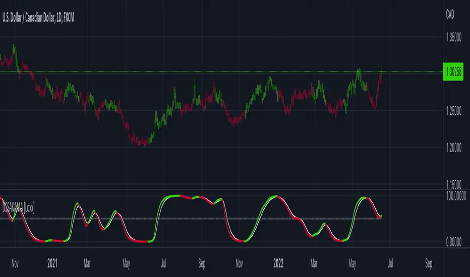
DSS of Advanced Kaufman AMA [Loxx]DSS of Advanced Kaufman AMA is a double smoothed stochastic oscillator using a Kaufman adaptive moving average with the option of using the Jurik Fractal Dimension Adaptive calculation. This helps smooth the stochastic oscillator thereby making it easier to identify reversals and trends.
What is the double smoothed stochastic?
The Double Smoothed Stochastic indicator was created by William Blau. It applies Exponential Moving Averages (EMAs) of two different periods to a standard Stochastic %K. The components that construct the Stochastic Oscillator are first smoothed with the two EMAs. Then, the smoothed components are plugged into the standard Stochastic formula to calculate the indicator.
What is KAMA?
Developed by Perry Kaufman, Kaufman's Adaptive Moving Average (KAMA) is a moving average designed to account for market noise or volatility . KAMA will closely follow prices when the price swings are relatively small and the noise is low. KAMA will adjust when the price swings widen and follow prices from a greater distance. This trend-following indicator can be used to identify the overall trend, time turning points and filter price movements.
What is the efficiency ratio?
In statistical terms, the Efficiency Ratio tells us the fractal efficiency of price changes. ER fluctuates between 1 and 0, but these extremes are the exception, not the norm. ER would be 1 if prices moved up 10 consecutive periods or down 10 consecutive periods. ER would be zero if price is unchanged over the 10 periods.
What is Jurik Fractal Dimension?
There is a weak and a strong way to measure the random quality of a time series.
The weak way is to use the random walk index ( RWI ). You can download it from the Omega web site. It makes the assumption that the market is moving randomly with an average distance D per move and proposes an amount the market should have changed over N bars of time. If the market has traveled less, then the action is considered random, otherwise it's considered trending.
The problem with this method is that taking the average distance is valid for a Normal (Gaussian) distribution of price activity. However, price action is rarely Normal, with large price jumps occuring much more frequently than a Normal distribution would expect. Consequently, big jumps throw the RWI way off, producing invalid results.
The strong way is to not make any assumption regarding the distribution of price changes and, instead, measure the fractal dimension of the time series. Fractal Dimension requires a lot of data to be accurate. If you are trading 30 minute bars, use a multi-chart where this indicator is running on 5 minute bars and you are trading on 30 minute bars.
Included
-Toggle bar colors on/offf
Parabolic SAR of KAMA [Loxx]Parabolic SAR of KAMA attempts to reduce noise and volatility from regular Parabolic SAR in order to derive more accurate trends. In addition, and to further reduce noise and enhance trend identification, PSAR of KAMA includes two calculations of efficiency ratio: 1) price change adjusted for the daily volatility; or, 2) Jurik Fractal Dimension Adaptive (explained below)
What is PSAR?
The parabolic SAR indicator, developed by J. Wells Wilder, is used by traders to determine trend direction and potential reversals in price. The indicator uses a trailing stop and reverse method called "SAR," or stop and reverse, to identify suitable exit and entry points. Traders also refer to the indicator as to the parabolic stop and reverse, parabolic SAR, or PSAR.
What is KAMA?
Developed by Perry Kaufman, Kaufman's Adaptive Moving Average (KAMA) is a moving average designed to account for market noise or volatility. KAMA will closely follow prices when the price swings are relatively small and the noise is low. KAMA will adjust when the price swings widen and follow prices from a greater distance. This trend-following indicator can be used to identify the overall trend, time turning points and filter price movements.
What is the efficiency ratio?
In statistical terms, the Efficiency Ratio tells us the fractal efficiency of price changes. ER fluctuates between 1 and 0, but these extremes are the exception, not the norm. ER would be 1 if prices moved up 10 consecutive periods or down 10 consecutive periods. ER would be zero if price is unchanged over the 10 periods.
What is Jurik Fractal Dimension?
There is a weak and a strong way to measure the random quality of a time series.
The weak way is to use the random walk index (RWI). You can download it from the Omega web site. It makes the assumption that the market is moving randomly with an average distance D per move and proposes an amount the market should have changed over N bars of time. If the market has traveled less, then the action is considered random, otherwise it's considered trending.
The problem with this method is that taking the average distance is valid for a Normal (Gaussian) distribution of price activity. However, price action is rarely Normal, with large price jumps occuring much more frequently than a Normal distribution would expect. Consequently, big jumps throw the RWI way off, producing invalid results.
The strong way is to not make any assumption regarding the distribution of price changes and, instead, measure the fractal dimension of the time series. Fractal Dimension requires a lot of data to be accurate. If you are trading 30 minute bars, use a multi-chart where this indicator is running on 5 minute bars and you are trading on 30 minute bars.
Conclusion from the combined efforts explained above:
-PSAR is a tool that identifies trends
-To reduce noise and identify trends during periods of low volatility, we calculate a PSAR on KAMA
-To enhance noise and reduction and trend identification, we attempt to derive an efficiency ratio that is less reliant on a Normal (Gaussian) distribution of price
Included:
-Customization of all variables
-Select from two different ER calculation styles
-Multiple timeframe enabled

Adaptive Oscillator constructor [lastguru]Adaptive Oscillators use the same principle as Adaptive Moving Averages. This is an experiment to separate length generation from oscillators, offering multiple alternatives to be combined. Some of the combinations are widely known, some are not. Note that all Oscillators here are normalized to -1..1 range. This indicator is based on my previously published public libraries and also serve as a usage demonstration for them. I will try to expand the collection (suggestions are welcome), however it is not meant as an encyclopaedic resource , so you are encouraged to experiment yourself: by looking on the source code of this indicator, I am sure you will see how trivial it is to use the provided libraries and expand them with your own ideas and combinations. I give no recommendation on what settings to use, but if you find some useful setting, combination or application ideas (or bugs in my code), I would be happy to read about them in the comments section.
The indicator works in three stages: Prefiltering, Length Adaptation and Oscillators.
Prefiltering is a fast smoothing to get rid of high-frequency (2, 3 or 4 bar) noise.
Adaptation algorithms are roughly subdivided in two categories: classic Length Adaptations and Cycle Estimators (they are also implemented in separate libraries), all are selected in Adaptation dropdown. Length Adaptation used in the Adaptive Moving Averages and the Adaptive Oscillators try to follow price movements and accelerate/decelerate accordingly (usually quite rapidly with a huge range). Cycle Estimators, on the other hand, try to measure the cycle period of the current market, which does not reflect price movement or the rate of change (the rate of change may also differ depending on the cycle phase, but the cycle period itself usually changes slowly).
Chande (Price) - based on Chande's Dynamic Momentum Index (CDMI or DYMOI), which is dynamic RSI with this length
Chande (Volume) - a variant of Chande's algorithm, where volume is used instead of price
VIDYA - based on VIDYA algorithm. The period oscillates from the Lower Bound up (slow)
VIDYA-RS - based on Vitali Apirine's modification of VIDYA algorithm (he calls it Relative Strength Moving Average). The period oscillates from the Upper Bound down (fast)
Kaufman Efficiency Scaling - based on Efficiency Ratio calculation originally used in KAMA
Deviation Scaling - based on DSSS by John F. Ehlers
Median Average - based on Median Average Adaptive Filter by John F. Ehlers
Fractal Adaptation - based on FRAMA by John F. Ehlers
MESA MAMA Alpha - based on MESA Adaptive Moving Average by John F. Ehlers
MESA MAMA Cycle - based on MESA Adaptive Moving Average by John F. Ehlers , but unlike Alpha calculation, this adaptation estimates cycle period
Pearson Autocorrelation* - based on Pearson Autocorrelation Periodogram by John F. Ehlers
DFT Cycle* - based on Discrete Fourier Transform Spectrum estimator by John F. Ehlers
Phase Accumulation* - based on Dominant Cycle from Phase Accumulation by John F. Ehlers
Length Adaptation usually take two parameters: Bound From (lower bound) and To (upper bound). These are the limits for Adaptation values. Note that the Cycle Estimators marked with asterisks(*) are very computationally intensive, so the bounds should not be set much higher than 50, otherwise you may receive a timeout error (also, it does not seem to be a useful thing to do, but you may correct me if I'm wrong).
The Cycle Estimators marked with asterisks(*) also have 3 checkboxes: HP (Highpass Filter), SS (Super Smoother) and HW (Hann Window). These enable or disable their internal prefilters, which are recommended by their author - John F. Ehlers . I do not know, which combination works best, so you can experiment.
Chande's Adaptations also have 3 additional parameters: SD Length (lookback length of Standard deviation), Smooth (smoothing length of Standard deviation) and Power ( exponent of the length adaptation - lower is smaller variation). These are internal tweaks for the calculation.
Oscillators section offer you a choice of Oscillator algorithms:
Stochastic - Stochastic
Super Smooth Stochastic - Super Smooth Stochastic (part of MESA Stochastic) by John F. Ehlers
CMO - Chande Momentum Oscillator
RSI - Relative Strength Index
Volume-scaled RSI - my own version of RSI. It scales price movements by the proportion of RMS of volume
Momentum RSI - RSI of price momentum
Rocket RSI - inspired by RocketRSI by John F. Ehlers (not an exact implementation)
MFI - Money Flow Index
LRSI - Laguerre RSI by John F. Ehlers
LRSI with Fractal Energy - a combo oscillator that uses Fractal Energy to tune LRSI gamma
Fractal Energy - Fractal Energy or Choppiness Index by E. W. Dreiss
Efficiency ratio - based on Kaufman Adaptive Moving Average calculation
DMI - Directional Movement Index (only ADX is drawn)
Fast DMI - same as DMI, but without secondary smoothing
If no Adaptation is selected (None option), you can set Length directly. If an Adaptation is selected, then Cycle multiplier can be set.
Before an Oscillator, a High Pass filter may be executed to remove cyclic components longer than the provided Highpass Length (no High Pass filter, if Highpass Length = 0). Both before and after the Oscillator a Moving Average can be applied. The following Moving Averages are included: SMA, RMA, EMA, HMA , VWMA, 2-pole Super Smoother, 3-pole Super Smoother, Filt11, Triangle Window, Hamming Window, Hann Window, Lowpass, DSSS. For more details on these Moving Averages, you can check my other Adaptive Constructor indicator:
The Oscillator output may be renormalized and postprocessed with the following Normalization algorithms:
Stochastic - Stochastic
Super Smooth Stochastic - Super Smooth Stochastic (part of MESA Stochastic) by John F. Ehlers
Inverse Fisher Transform - Inverse Fisher Transform
Noise Elimination Technology - a simplified Kendall correlation algorithm "Noise Elimination Technology" by John F. Ehlers
Except for Inverse Fisher Transform, all Normalization algorithms can have Length parameter. If it is not specified (set to 0), then the calculated Oscillator length is used.
More information on the algorithms is given in the code for the libraries used. I am also very grateful to other TradingView community members (they are also mentioned in the library code) without whom this script would not have been possible.
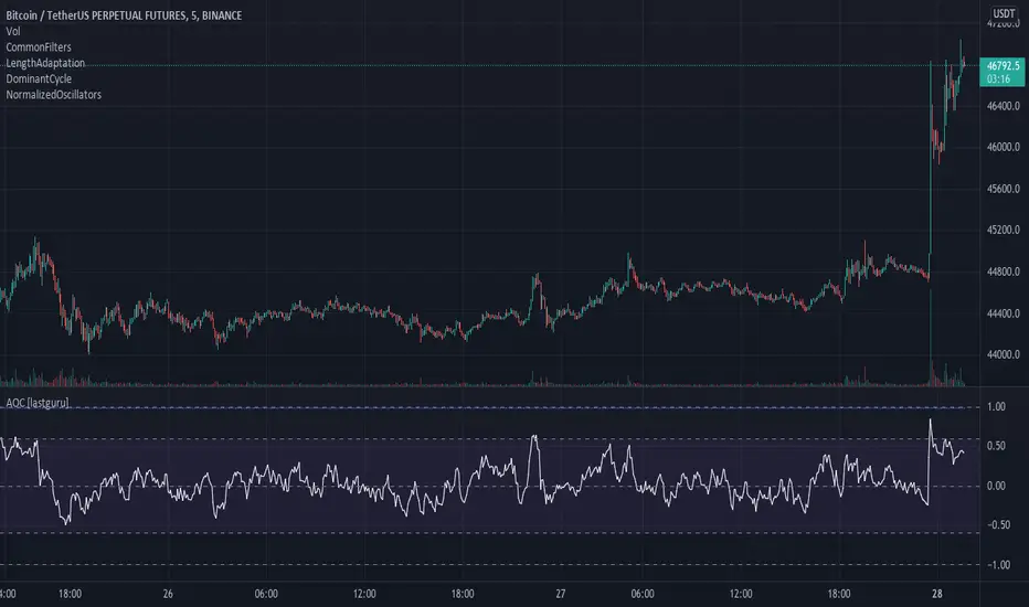
poopivs [ULTIMATE PIVOT HIGHS AND LOWS]Big thanks to @LudaCode for the missing pivots script. Carried my dumpy trucky badoinkadoink.
This is an elevated pivot script that follows the 3 candle pivot rule (strictly) and does not miss pivots like williams fractals.
Missing pivots marked by transparent circles are derived pivots, giving you a higher resolution for price action.
Colored bars show potential problem areas for pivots (drawing zigzags in particular) and indicate a pivot high and low on the same candle.
Will potentially upgrade this script to include auto zig zags, trend, and intermediate highs and lows finder.
Let me know if you have any suggestions ideas in the comments.
Best,
P

Liquidity RaidThe market always seeks liquidity. Liquidity rests above previous highs and below previous lows.
The script highlights the breach of a market structure high or low (W/D/4H/1H), and will alert you on the first fractal break in the opposite direction.
The idea is that the raid happens, and you are only alerted once a candle breaks a fractal and closes in the opposite direction.
When a signal is printed, it does not mean to enter immediately. It just means that there is a fractal break in the opposite direction, and that you will need to assess current price action and market structure for a potential trade on pullback.
You still need to take HTF directional bias, market structure, order blocks and imbalances into consideration.
The script is for trading on on smaller time frames (1/2/3/5m).
Fractal periods, lines and colours are all customizable

Support & Ressistance by @kaleboraciy [REUPLOAD]█ OVERVIEW
Support & Resistance levels are important in trading as we all know.
█ WARNING
This version is beta, maybe sometimes it will plot wrong levels, but i will try to to eliminate these issues. And please note, that you should find your own ideal settings for every ticker you use.
█ FEATURES
This is the first script in Pine Community which plots levels using the last two points/ pivots /fractals.
It also stops plotting levels when there is a breakout on the particular level.
█ SETTINGS
1. Pivot Points Length - defines pivot points length. Using to find points where market is reversed. If you set lower value, there will be more points but less useful. As I said you should find your optimal parameters.
2. Inaccuracy in % - defines maximal possible inaccuracy between 2 pivot points .
3. Linewidth - width of line(level)
4. Start Calculations from - if you use low timeframe (1m - 30m) there are a lot of calculations, and PineScript can't process it. This parameter defines start date of calculations and now there are less data and Pine can process it better.
█ HOW IT WORKS
When a new pivot appears, it draws invisible line starting in this pivot . when the second pivots gets created, it checks all lines in array. When inaccuracy is smaller than defined, the line becomes visible.
If price breaks trough the pivots , the lines stop and a new cycle begins.
I hope that this script will be helpful in your trading🙂

Support & Resistance LevelsPlots support and resistance levels based on occurrence of fractals.
Line width indicates historical significance of the level.
Decreasing the proximity multiplier input increases the sensitivity/ increases the frequency of level changes.
If price closes above a resistance level, the level becomes a support level and its color on the chart changes to green (& vice-versa).

Stop Hunt (Nephew_Sam_)Finds and plots stop hunts / raids between fractal points.
If a candle wicks above/below a fractal and close back in its range, it will plot a line and/or dot based on preference.
Also able to filter a time period, meaning it will only plot if the stop hunt happened inside the time period.
Other options:
- Draw fractal points
- Choose between 3 or 5 bar fractal
- Set how far back you want to check for a stop hunt
- Change line color

[blackcat] L2 Ehlers Hurst Coefficient IndicatorLevel: 2
Background
John F. Ehlers introuced Hurst Coefficient Indicator in his "Cycle Analytics for Traders" chapter 6 on 2013.
Function
The Hurst coefficient is one way to attempt to get a handle on the slope of the power density of market data. The Hurst coefficient varies between 0 and 1, and is related to the α power coefficient as H = 1 − α/2. The Hurst coefficient is more estimated than computed. Dr. Ehlers found the estimate using the fractal dimension was the most practical for shorter-term market data. The Hurst coefficient is related to the fractal dimension as H = 2 − D. Dr. Ehlers would like to make it perfectly clear that the Hurst coefficient or the fractal dimension has no direct practical application to trading not only because it is an estimate, but also because it has no predictive value. These computations only reflect the general structure of the market, and the answer you get is dependent on your assumptions. For example, the Hurst coefficient changes dramatically with the length of data used in making the estimate.
The only user input is the length of data to be used. The number can be arbitrarily large if you have sufficient data. The results are critically dependent on the input data length selected. After declaring variables, the coefficients of a 20-bar SuperSmoother filter are computed. The computations of N1, N2, and N3 are as described in the previous section. The fractal dimension is then converted to the Hurst coefficient, which is subsequently smoothed in the SuperSmoother filter.
Key Signal
SmoothHurst --> Hurst Coefficient Indicator fast line
Trigger --> Hurst Coefficient Indicator slow line
Pros and Cons
100% John F. Ehlers definition translation of original work, even variable names are the same. This help readers who would like to use pine to read his book. If you had read his works, then you will be quite familiar with my code style.
Remarks
The 40th script for Blackcat1402 John F. Ehlers Week publication.
Readme
In real life, I am a prolific inventor. I have successfully applied for more than 60 international and regional patents in the past 12 years. But in the past two years or so, I have tried to transfer my creativity to the development of trading strategies. Tradingview is the ideal platform for me. I am selecting and contributing some of the hundreds of scripts to publish in Tradingview community. Welcome everyone to interact with me to discuss these interesting pine scripts.
The scripts posted are categorized into 5 levels according to my efforts or manhours put into these works.
Level 1 : interesting script snippets or distinctive improvement from classic indicators or strategy. Level 1 scripts can usually appear in more complex indicators as a function module or element.
Level 2 : composite indicator/strategy. By selecting or combining several independent or dependent functions or sub indicators in proper way, the composite script exhibits a resonance phenomenon which can filter out noise or fake trading signal to enhance trading confidence level.
Level 3 : comprehensive indicator/strategy. They are simple trading systems based on my strategies. They are commonly containing several or all of entry signal, close signal, stop loss, take profit, re-entry, risk management, and position sizing techniques. Even some interesting fundamental and mass psychological aspects are incorporated.
Level 4 : script snippets or functions that do not disclose source code. Interesting element that can reveal market laws and work as raw material for indicators and strategies. If you find Level 1~2 scripts are helpful, Level 4 is a private version that took me far more efforts to develop.
Level 5 : indicator/strategy that do not disclose source code. private version of Level 3 script with my accumulated script processing skills or a large number of custom functions. I had a private function library built in past two years. Level 5 scripts use many of them to achieve private trading strategy.
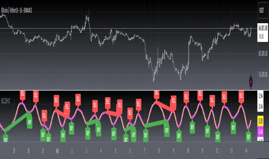
Candlestick Pattern Detector - Aitch-TThis script detects the following candlestick patterns:
Bullish Patterns:
- Normal 3 Bar Fractal
- Enhanced 3 Bar Fractal
- Engulfing
- Harami ( Inside bar )
- Bullrami (Altenate Bull Harami)
Bearish Patterns:
- Normal 3 Bar Fractal
- Enhanced 3 Bar Fractal
- Engulfing
- Harami ( Inside bar )
- Bearami (Alternate Bear Harami)
- Shooting Star
How it works:
- When you add the script to your chart, green and red dots will appear at the top and the bottom of the chart.
- Red dots at the top of the chart point out the candles that have completed a bearish pattern .
- Green dots at the bottom of the chart point out the candles that have completed a bullish pattern .
How to use:
Use it in conjunction with other analysis tools ( Fibonacci Retracements, Histogram, Willy, RSI , volume , etc) to determine high probability levels.

Quadratic SemaphoreThe quadratic semaphore indicator is an indicator that find confirmed market u-turn with the help of 2 quadratic regression calculated with Highs and Lows over the last “length” periods.
- “p” setting is candlesticks quantity to confirmed the quadratic regression has formed a High or Low parabola, such as Fractals. Consecutive same signals can happen due to the use of different price values for upper and lower semaphore.
- Adjust the settings to your instrument and time frame.
- Alerts included.
Success with your trade¡¡
Assassin Zenzen about top fractal and bottom fractal
show top fractal and bottom fractal
---
TODO
Contain Kline , Tradingview pine not support yet.

CCI Highlighted & Divergence Signals [CryptoProSignal]>> This is the updated version of my previous ' CCI Highlighted ' indicator/oscillator (checkout in my previous published scripts) .
> > Whats new :
> This version of CCI highlighted has integrated divergence signals to spot various divergences on any timeframe which ultimately saves your time rather than
spotting divergences by manual analysis. Thus making it CCI Highlighted & Divergence Signals indicator/oscillator.
> By default it is optimised to give you divergence signal whenever CCI Length1 is above 100 or below -100 but you can always enable all divergences in
setting/format by simple check/uncheck.
> Tag reference in indicator/oscillator :
* Tag "R" refers to Regular divergence.
* Tag "H" refers to Hidden divergence.
----------------------------------------------------------------------------------------------------------------------------------------------------------------------
----------------------------------------------------------------------------------------------------------------------------------------------------------------------
***Below is the description copy pasted from my previous version of CCI Highlighted for remaining functionality of this updated indicator/oscillator.***
>> This script is purely based on Commodity Channel Index ( CCI ) with multiple CCI instances being used within one oscillator.
>> User can use as much as 5 CCI instances/plot within one oscillator.
> How to use :
1. When Bullish :
Whenever CCI length 14 crosses above -100(negative 100) that means bullish momentum is supported.
Best bullish/long entry would be when CCI length 14 crosses above -100(negative 100) as mentioned above and at the same time CCI length
200 is bouncing on top of +100(positive 100).
2. When Bearish :
Whenever CCI length 14 crosses below +100(positive 100) that means bearish momentum is supported .
Best bearish/short entry would be when CCI length 14 crosses below +100(positive 100) as mentioned above and at the same time CCI length
200 is bouncing at bottom of -100(negative 100) .
> Color Clarity :
a. Bullish support is highlighted GREEN and bearish support is highlighted RED within the oscillator background with respect to
Length 1 (i.e 14 by default) .
b. PURPLE is highhighted when Length 5(i.e 200 by default) is bouncing either on top of +100(for bullish ) or at bottom of -100(for bearish ).
c. AQUA is highlighted when Length 3(i.e 50 by default) is bouncing on top or at bottom of 0 from either side respectively.
d. Best entry in both cases i.e bullish or bearish as mentioned above('How to use') is highlighted WHITE by default.
> Tip:
Just observe the color outputs on any timeframe in a chart as it works fractally on every timeframe , it will help you understand better with
clarity.
> You are always free to experiment with the CCI lengths, change highlighted color and hide/unhide the Lengths as per your requirements in
setting/format .
