CCI Highlighted [ankit4349]>> This script is purely based on Commodity Channel Index (CCI) with multiple CCI instances being used within one oscillator.
>> User can use as much as 5 CCI instances/plot within one oscillator.
> How to use :
1. When Bullish :
Whenever CCI length 14 crosses above -100(negative 100) that means bullish momentum is supported.
Best bullish/long entry would be when CCI length 14 crosses above -100(negative 100) as mentioned above and at the same time CCI length
200 is bouncing on top of +100(positive 100).
2. When Bearish :
Whenever CCI length 14 crosses below +100(positive 100) that means bearish momentum is supported .
Best bearish/short entry would be when CCI length 14 crosses below +100(positive 100) as mentioned above and at the same time CCI length
200 is bouncing at bottom of -100(negative 100) .
> Color Clarity :
a. Bullish support is highlighted GREEN and bearish support is highlighted RED within the oscillator background with respect to
Length 1 (i.e 14 by default) .
b. PURPLE is highhighted when Length 5(i.e 200 by default) is bouncing either on top of +100(for bullish) or at bottom of -100(for bearish).
c. AQUA is highlighted when Length 3(i.e 50 by default) is bouncing on top or at bottom of 0 from either side respectively.
d. Best entry in both cases i.e bullish or bearish as mentioned above('How to use') is highlighted WHITE by default.
> Tip:
Just observe the color outputs on any timeframe in a chart as it works fractally on every timeframe , it will help you understand better with
clarity.
> You are always free to experiment with the CCI lengths, change highlighted color and hide/unhide the Lengths as per your requirements in
setting/format .
Cari dalam skrip untuk "Fractal"

(JS) RSI Divergence Volume Weighted (v1.1)Okay so I added all kinds of stuff - not sure you've ever been able to customize RSI like this before. The goal here was to allow the user to be able to play around and find the RSI formula that suits them the best.
There's still the obvious features from version 1.0 which are RSI Length and Relative Volume Length, but I really expanded upon the first one. Here's the list of new features:
- RSI Input: 0-6 are the options and they allow you to use - Close, Open, High, Low, HL2, HLC3, and OHLC4. Now you can plug any of these choices into the RSI formula.
- RV x Divergence?: This is how I calculated the original formula, but you can leave this unchecked to turn Relative Volume off, or apply elsewhere.
- RV x RS?: Another way to calculate the function. There's two sides, Divergence RS and Standard RS - these check marks allow you to select which part you prefer to be multiplied by Relative Volume. Check neither to turn off RV multiplication, check both to add it on both sides of the equation.
* Relative Volume Note - when looking at longer term charts, be aware that if a candle JUST began, it's obviously going to have really low RV and will throw off the current candle (which is why I added the option to turn off/on). Best usage is at candle close (or ignore the current candle).
-Divergence Weight: So as it stands, the Standard RS and Divergence RS are both equal weight ( /2). This allows you to change the weight at increments of 0.1 on a scale of 0-2. Making 2 purely Divergence, and 0 purely Standard RSI. With RV left off on both options, and a weight setting of 0, this becomes a regular RSI again.
-SMA Divergence?: This is the option to leave the Divergence equation unsmooth, or to smooth it over. SMA is an unsmoothed average, whereas leaving it unchecked runs it through an RMA smoothing the same way standard RSI is calculated.
-Fractal Divergence Lines: I added fractal lines to spot divergence in the indicator vs. the price. This was meant to help you spot divergence easier.
-Show Fractal Labels?: This adds "Bull" and "Bear" labels on said divergence.
-Show Fractal Channel?: This allows you to see the whole fractal channel.
-Added Horizontals: I added horizontal lines at 40 and 60, to make viewing the RSI values a bit easier.
-Added Trend BG: I also added a feature where the BG color will change with the ongoing trend. I removed the previous colors I had in the BG.
Enjoy!

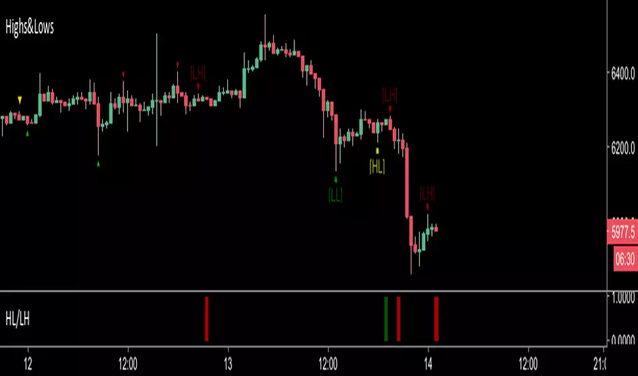
Highs&LowsShows Higher Highs, Higher Lows, Lower Lows & Lower Highs based off of Bill Williams fractals.
I use this mainly by shorting a break of the higher lows marked in yellow.
A long signal would be a candle close above a lower high (less reliable)
Alerts can be set with the secondary indicator below the chart.
Higher Lows / Lower Highs Alerts -https://www.tradingview.com/script/Ka1yXqRj-Higher-Lows-Lower-Highs-Alerts/
RSI & Volume Based S&R LinesRSI & Volume Based S&R Lines V1.0
Inspired by previous work available on TradingView I wanted to create my own Support & Resistance based indicator to help with confirming signals used with my swing trading tools (also available on TV).
There are two support and resistance lines, one RSI & historic price based and the other based on volume fractals. I've previously used these to help confirm entries previously and the fundamentals behind it are simple but effective.
Access
This indicator is completely free to those part of my discord community
Link: discord.gg

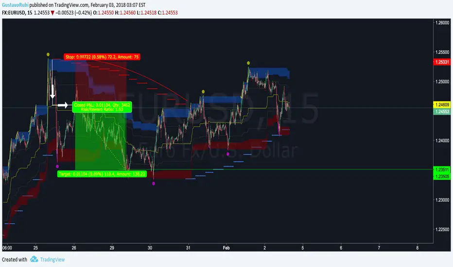
BullTrading 15m Trend master V3.0
BullTrading 15m Trend master V3.0 is a Retracement Trading System that filters main trends with minimum lag. This trading system is based on Transient Zones Theory, Market Makers Theory and Fractals.
BullTrading 15m Trend master V3.0 is alert friendly and works on any financial instrument.
White lines and arrows are manually drawn to show how to calculate the Optimum Entry Levels.
Initial SL is calculated by adding 3 pips to the nearest BullTrading Parabolic SAR line.
TP 1 formula is calculated by multiplying by 1.5 the initial SL pips.
TP 2 is Open and trailed 3 pips above the last BullTrading Parabolic SAR line.
BE is set after reaching the initial SL pips or by trailing the last BullTrading Parabolic SAR line plus 3 pips.
BullTrading 15' Trend MasterBullTrading TrendMaster is a non repainting Experimental Indicator for 15m timeframes.
It has Optional Signal and Alerting functions. Entries are recommended using Fibo retracements for optimal entry levels. If the pullback is not strong enough to activate our limit pending order, you can use stop pending orders above/below fractals. Use the BullTrading P-SAR for SL placing and Trailing Profits.
If you don't like arrows signalas just remove them and use the indicator as very accurate trend confirmation tool following this criteria:
Confirmed Uptrends are marked when the BullTrading P-SAR is Lime Green AND the Moving Average is Lime Green as well (Opposite for Downtrends).
Drop me a line for feedback and improvement.
Enjoy and Happy Trading

Patrones de entrada/salida V.1.0 -BETA-Este algoritmo intenta identificar patrones o fractales dentro de los movimientos de precios para dar señales de compra o venta de activos.

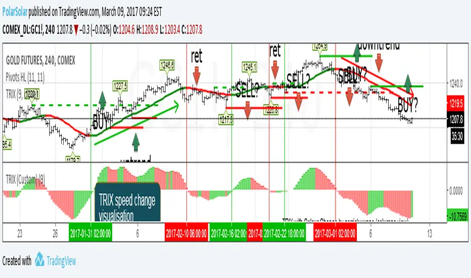
Triple Exponental Moving Average (overlay)TRIX Overlay + TRIX change Histogramm = simplest tactic to trade.
Just use last counter trend fractal to place delayed order
A counter trend fractal is a fractal down on TRIX uptrend or fractal up on TRIX downtrend.
Use TRIX speed change histogramm to seek divergence
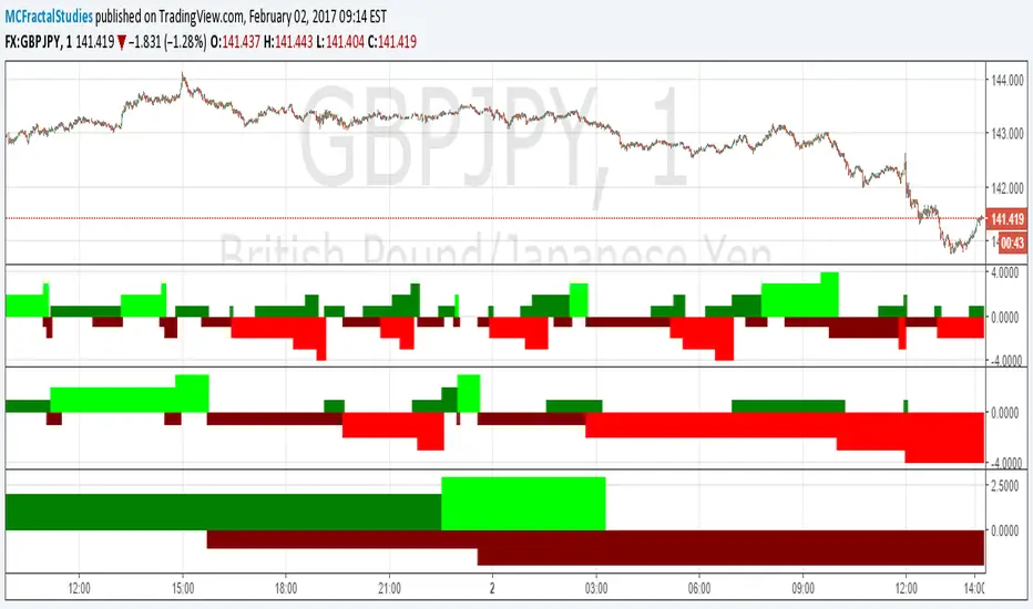
MC Market StructureMC Market Structure © is one of the five MC Fractal Studies ©
MC Fractal Studies (c) disassemble the market data in an objective way and organize charts information in order to identify all the various Waves on all the various fractal scales, that make up the typical market charts, and show them to the eyes of investors in an inclusive but detailed way.
The ability to view and examine the multi-scale fractal market structure of a chart can immensely help an investor, giving him an edge that can be used to increase trading performance.

MC Waves OscillatorMC Waves Oscillator © is one of the five MC Fractal Studies ©
MC Fractal Studies (c) disassemble the market data in an objective way and organize charts information in order to identify all the various Waves on all the various fractal scales, that make up the typical market charts, and show them to the eyes of investors in an inclusive but detailed way.
The ability to view and examine the multi-scale fractal market structure of a chart can immensely help an investor, giving him an edge that can be used to increase trading performance.

MC Waves SizeMC Waves Size © is one of the five MC Fractal Studies ©
MC Fractal Studies (c) disassemble the market data in an objective way and organize charts information in order to identify all the various Waves on all the various fractal scales, that make up the typical market charts, and show them to the eyes of investors in an inclusive but detailed way.
The ability to view and examine the multi-scale fractal market structure of a chart can immensely help an investor, giving him an edge that can be used to increase trading performance.

MC Wave Structure OnChartMC Wave Structure OnChart © is one of the five MC Fractal Studies ©
MC Fractal Studies (c) disassemble the market data in an objective way and organize charts information in order to identify all the various Waves on all the various fractal scales, that make up the typical market charts, and show them to the eyes of investors in an inclusive but detailed way.
The ability to view and examine the multi-scale fractal market structure of a chart can immensely help an investor, giving him an edge that can be used to increase trading performance.

MC Market Structure OscillatorMC Market Structure Oscillator © is one of the five MC Fractal Studies ©
MC Fractal Studies (c) disassemble the market data in an objective way and organize charts information in order to identify all the various Waves on all the various fractal scales, that make up the typical market charts, and show them to the eyes of investors in an inclusive but detailed way.
The ability to view and examine the multi-scale fractal market structure of a chart can immensely help an investor, giving him an edge that can be used to increase trading performance.
Quantum EdgeQuantum Edge
DESCRIPTION:
Time-based cycle alignment scanner using fractal cycle theory to detect when multiple timing cycles converge at mathematically significant zones.
█ OVERVIEW
Quantum Edge is a time-based cycle alignment scanner built on fractal cycle theory. Markets move in nested cycles across multiple timeframes. This indicator detects moments when several of these cycles simultaneously reach mathematically significant positions, creating potential turning points.
The core concept: when multiple independent timing cycles converge at key zones, the probability of a reaction increases. The more cycles aligned, the higher the probability score.
█ HOW IT WORKS
The indicator tracks multiple time-based cycles of varying lengths. Each cycle is analyzed for its current position within its phase. When a cycle reaches a statistically significant zone (based on cycle theory), it contributes points to a composite probability score.
Shorter cycles contribute fewer points (they align frequently).
Longer cycles contribute more points (they align rarely).
Additional weighting is applied for:
- Specific days of the week known for higher volatility
- Specific times of day associated with market structure shifts
The final score represents how many timing factors are currently aligned.
█ SIGNALS EXPLAINED
👑 Rare multi-cycle convergence — Several long-duration cycles aligned simultaneously. Occurs a few times per month.
💎 Strong convergence — Multiple mid-to-long duration cycles aligned. Occurs a few times per week.
🌅 Daily cycle alignment — Daily-length cycle at a key zone with supporting factors. Occurs 1-2 times per day.
🔥 Short cycle alignment — Shorter-duration cycles aligned. Occurs several times per day.
🔮 Prediction — The indicator scans ahead and displays where future alignments are likely to occur based on the deterministic nature of time cycles.
█ TRADING MODES
The indicator includes preset modes that adjust sensitivity:
SNIPER — Only displays the highest-scoring alignments. For patient traders waiting for the best setups.
DAILY — Displays daily-quality alignments and above. Recommended starting point for most traders.
ACTIVE — Displays more frequent setups. For traders who want more opportunities and can filter with price analysis.
SCALP — Displays all qualifying alignments. Highest frequency, requires additional confirmation.
█ WHAT MAKES THIS UNIQUE
This indicator uses a proprietary weighted scoring system based on fractal cycle mathematics. The specific cycle lengths, zone calculations, and weighting factors are the result of extensive research into cyclical market behavior.
The predictive feature is deterministic — because time cycles are mathematical, future alignments can be calculated in advance. This allows traders to plan entries before setups occur rather than reacting after the fact.
The source is protected because the specific parameters and scoring logic represent significant research and development.
█ INTENDED USE
This is a TIMING tool, not a directional signal generator.
It answers: "When are multiple cycles aligned?"
It does NOT answer: "Which direction should I trade?"
Combine with your own price analysis (support/resistance, order flow, market structure) to determine direction. Use this tool to identify WHEN those setups have higher probability.
█ LIMITATIONS
- No indicator predicts the future with certainty
- Cycle alignments indicate probability, not guaranteed outcomes
- Past alignment results do not guarantee future performance
- This tool requires combination with price-based analysis for best results
- Not all alignments result in tradeable moves
█ SETTINGS
- Mode Selection: Choose your preferred sensitivity level
- Show Score: Toggle probability scores on/off
- Show Predictions: Toggle future alignment predictions on/off
- Prediction Range: How far ahead to scan for alignments
- Colors: Customize signal colors to your preference
█ MARKETS AND TIMEFRAMES
Works on any liquid market: Futures, Forex, Crypto, Stocks, Indices.
Optimized for intraday timeframes (1-15 minute charts) but can be applied to higher timeframes for swing trading applications.
█ ACCESS
This is an invite-only script. If you have questions about the methodology or would like to discuss access, you may send me a direct message.

Kinetic Elasticity Reversion System - Adaptive Genesis Engine🧬 KERS-AGE - EVOLVED KINETIC ELASTICITY REVERSION SYSTEM
EDUCATIONAL GUIDE & THEORETICAL FOUNDATION
⚠️ IMPORTANT DISCLAIMER
This indicator and guide are provided for educational and informational purposes only. This is NOT financial advice, investment advice, or a recommendation to buy or sell any security.
Trading involves substantial risk of loss. Past performance does not guarantee future results. The performance metrics, win rates, and examples shown are from historical backtesting and do not represent actual trading results. Always conduct your own research, paper trade extensively, and never risk capital you cannot afford to lose.
The developers assume no responsibility for any trading losses incurred through use of this indicator.
INTRODUCTION
KERS-AGE (Kinetic Elasticity Reversion System - Adaptive Genetic Evolution) represents an educational exploration of adaptive trading systems. Unlike traditional indicators with fixed parameters, KERS-AGE demonstrates a dynamic, evolving approach that adjusts to market conditions through genetic algorithms and machine learning techniques.
This guide explains the theoretical concepts, technical implementation, and educational examples of how the system operates.
CONCEPTUAL FRAMEWORK
Traditional Indicators vs. Adaptive Systems:
Traditional Indicators:
Fixed parameters
Single strategy approach
Static behavior
Designed for specific conditions
Require manual optimization
Adaptive System Approach (KERS-AGE):
Dynamic parameters (adjust based on conditions)
Multiple strategies tested simultaneously
Pattern recognition (cluster analysis)
Regime-aware (speciation)
Automated optimization (genetic algorithms)
Transparent operation (detailed dashboard)
CORE CONCEPTS EXPLAINED
1. THE ELASTICITY ANALOGY 🎯
The indicator models price behavior as if connected to a moving average by an elastic band:
Price extends away → Elastic tension builds → Potential reversion point identified
Key Measurements:
STRETCH: Distance from price to equilibrium (MA)
TENSION: Normalized force calculation
THRESHOLD: Point where multiple factors align
Theoretical Foundation:
Markets have historically shown mean-reverting tendencies around fair value. This concept quantifies the deviation and identifies potential reversal zones based on multiple confluence factors.
Mathematical Approach:
text
Tension Score = (Price Distance from MA) / (Band Width) × Volatility Scaling
Signal Threshold = Multiple of ATR × Dynamic Volatility Ratio
Confluence = Tension Score + Additional Factors
2. THE 6 SIGNAL TYPES 📊
The system recognizes 6 distinct pattern categories:
A. ELASTIC SIGNALS
Pattern: Price reaches statistical band extremes
Theory: Maximum deviation from mean suggests potential reversion
Detection: Price touches outer zones (typically 2-3× ATR from MA)
Component: Mathematical band extension measurement
Historical Context: Often observed in markets with clear swing patterns
B. WICK SIGNALS
Pattern: Extended rejection wicks on candles
Theory: Failed breakout attempts may indicate directional exhaustion
Detection: Upper/lower wick exceeding 2× body size
Component: Real-time price rejection measurement
Historical Context: Common in volatile conditions with rapid reversals
C. EXHAUSTION SIGNALS
Pattern: Decelerating momentum despite price extension
Theory: Velocity and acceleration divergence may precede reversals
Detection: Decreasing velocity with negative acceleration
Component: Momentum derivative analysis
Historical Context: Often seen at trend maturity points
D. CLIMAX SIGNALS
Pattern: Volume spike at price extreme
Theory: Unusual volume at extremes historically correlates with turning points
Detection: Volume 1.5-2.5× average at band extreme
Component: Volume-price relationship analysis
Historical Context: Associated with institutional activity or capitulation
E. STRUCTURE SIGNALS
Pattern: Fractal pivot formations (swing highs/lows)
Theory: Market structure points have historically acted as support/resistance
Detection: 2-4 bar pivot patterns
Component: Classical technical analysis
Historical Context: Universal across timeframes and markets
F. DIVERGENCE SIGNALS
Pattern: RSI divergence versus price
Theory: Momentum divergence has historically preceded price reversals
Detection: Price makes new extreme but RSI does not
Component: Oscillator divergence detection
Historical Context: Considered a leading indicator in technical analysis
Pattern Confluence:
Historical testing suggests stronger signals when multiple types align:
Elastic + Wick + Volume = Higher confluence score
Elastic + Exhaustion + Divergence = Multiple confirmation factors
Any 3+ types = Increased pattern strength
Note: Past pattern performance does not guarantee future occurrence.
3. REGIME DETECTION 🌍
The system attempts to classify market conditions into three behavioral regimes:
📈 TREND REGIME
Detection Methodology:
text
Efficiency Ratio = Net Movement / Total Movement
Classification: Efficiency > 0.5 AND Volatility < 1.3 → TREND
Characteristics Observed:
Directional price movement
Relatively lower volatility
Defined higher highs/lower lows
Persistent directional momentum
System Response:
Reduces signal frequency
Prioritizes trend-specialist strategies
Applies additional filtering to counter-trend signals
Increases confluence requirements
Educational Note:
In trending conditions, counter-trend mean reversion signals historically have shown reduced reliability. Users may consider additional confirmation when trend regime is detected.
↔️ RANGE REGIME
Detection Methodology:
text
Classification: Efficiency < 0.5 AND Volatility 0.9-1.4 → RANGE
Characteristics Observed:
Oscillating price action
Defined support/resistance zones
Mean-reverting behavior patterns
Relatively balanced directional flow
System Response:
Increases signal frequency
Activates range-specialist strategies
Adjusts bands relative to volatility
Reduces confluence threshold
Educational Note:
Historical backtesting suggests mean reversion systems have performed better in ranging conditions. This does not guarantee future performance.
🌊 VOLATILE REGIME
Detection Methodology:
text
Classification: DVS (Dynamic Volatility Scaling) > 1.5 → VOLATILE
Characteristics Observed:
Erratic price swings
Expanded ranges
Elevated ATR readings
Often news or event-driven
System Response:
Activates volatility-specialist strategies
Widens bands automatically
Prioritizes wick rejection signals
Emphasizes volume confirmation
Educational Note:
Volatile conditions historically present both opportunity and increased risk. Wider stops may be appropriate for risk management.
4. GENETIC EVOLUTION EXPLAINED 🧬
The system employs genetic algorithms to optimize parameters - an approach used in computational finance research.
The Evolution Process:
STEP 1: INITIALIZATION
text
Initial State: System creates 4 starter strategies
- Strategy 0: Range-optimized parameters
- Strategy 1: Trend-optimized parameters
- Strategy 2: Volatility-optimized parameters
- Strategy 3: Balanced parameters
Each contains 14 adjustable parameters (genes):
- Band sensitivity
- Extension multiplier
- Wick threshold
- Momentum threshold
- Volume multiplier
- Component weights (elastic, wick, momentum, volume, fractal)
- Target percentage
STEP 2: COMPETITION (Shadow Trading)
text
Early Bars: All strategies generate signals in parallel
- Each tracks hypothetical performance independently
- Simulated P&L, win rate, Sharpe ratio calculated
- No actual trades executed (educational simulation)
- Performance metrics recorded for analysis
STEP 3: FITNESS EVALUATION
text
Fitness Calculation =
0.25 × Win Rate +
0.25 × PnL Score +
0.15 × Drawdown Score +
0.30 × Sharpe Ratio Score +
0.05 × Trade Count Score
With Walk-Forward enabled:
Fitness = 0.60 × Test Score + 0.40 × Train Score
With Speciation enabled:
Fitness adjusted by Diversity Penalty
STEP 4: SELECTION (Tournament)
text
Periodically (default every 50 bars):
- Randomly select 4 active strategies
- Compare fitness scores
- Top 2 selected as "parents"
STEP 5: CROSSOVER (Breeding)
text
Parent 1 Fitness: 0.65
Parent 2 Fitness: 0.55
Weight calculation: 0.65/(0.65+0.55) = 54%
For each parameter:
Child Parameter = (0.54 × Parent1) + (0.46 × Parent2)
Example:
Band Sensitivity: (0.54 × 1.5) + (0.46 × 2.0) = 1.73
STEP 6: MUTATION
text
For each parameter:
if random(0-1) < Mutation Rate (default 0.15):
Add random variation: -12% to +12%
Purpose: Prevents premature convergence
Enables: Discovery of novel parameter combinations
ADAPTIVE MUTATION:
If population fitness converges → Mutation rate × 1.5
(Encourages exploration when diversity decreases)
STEP 7: INSERTION
text
New strategy added to population:
- Assigned unique ID number
- Generation counter incremented
- Begins shadow trading
- Competes with existing strategies
STEP 8: CULLING (Selection Pressure)
text
Periodically (default every 100 bars):
- Identify lowest fitness strategy
- Verify not elite (protected top performers)
- Verify not last of species
- Remove from population
Result: Maintains selection pressure
Effect: Prevents weak strategies from diluting signals
STEP 9: SIGNAL GENERATION LOGIC
text
When determining signals to display:
If Ensemble enabled:
- All strategies cast weighted votes
- Weights based on fitness scores
- Specialists receive boost in matching regime
- Signal generated if consensus threshold reached
If Ensemble disabled:
- Single highest-fitness strategy used
STEP 10: ADAPTATION OBSERVATION
text
Over time: Population characteristics may shift
- Lower-performing strategies removed
- Higher-performing strategies replicated
- Parameters adjust toward observed optima
- Fitness scores generally trend upward
Long-term: Population reaches maturity
- Strategies become specialized
- Parameters optimized for recent conditions
- Performance stabilizes
Educational Context:
Genetic algorithms are a recognized computational method for optimization problems. This implementation applies those concepts to trading parameter optimization. Past optimization results do not guarantee future performance.
5. SPECIATION (Niche Specialization) 🐟🦎🦅
Inspired by biological speciation theory applied to algorithmic trading.
The Three Species:
RANGE SPECIALISTS 📊
text
Optimized for: Sideways market conditions
Parameter tendencies:
- Tighter bands (1.0-1.5× ATR)
- Higher sensitivity to elastic stretch
- Emphasis on fractal structure
- More frequent signal generation
Typically emerge when:
- Range regime detected
- Clear support/resistance present
- Mean reversion showing historical success
Historical backtesting observations:
- Win rates often in 55-65% range
- Smaller reward/risk ratios (0.5-1.5R)
- Higher trade frequency
TREND SPECIALISTS 📈
text
Optimized for: Directional market conditions
Parameter tendencies:
- Wider bands (2.0-2.5× ATR)
- Focus on momentum exhaustion
- Emphasis on divergence patterns
- More selective signal generation
Typically emerge when:
- Trend regime detected
- Strong directional movement observed
- Counter-trend exhaustion signals sought
Historical backtesting observations:
- Win rates often in 40-55% range
- Larger reward/risk ratios (1.5-3.0R)
- Lower trade frequency
VOLATILITY SPECIALISTS 🌊
text
Optimized for: High-volatility conditions
Parameter tendencies:
- Expanded bands (1.5-2.0× ATR)
- Priority on wick rejection patterns
- Strong volume confirmation requirement
- Very selective signals
Typically emerge when:
- Volatile regime detected
- High DVS ratio (>1.5)
- News-driven or event-driven conditions
Historical backtesting observations:
- Win rates often in 50-60% range
- Variable reward/risk ratios (1.0-2.5R)
- Opportunistic trade timing
Species Protection Mechanism:
text
Minimum Per Species: Configurable (default 2)
If Range specialists = 1:
→ Preferential spawning of Range type
→ Protection from culling process
Purpose: Ensures coverage across regime types
Theory: Markets cycle between behavioral states
Goal: Prevent extinction of specialized approaches
Fitness Sharing:
text
If Species has 4 members:
Individual Fitness × 1 / (4 ^ 0.3)
Individual Fitness × 0.72
Purpose: Creates pressure toward species diversity
Effect: Prevents single approach from dominating population
Educational Note: Speciation is a theoretical framework for maintaining strategy diversity. Past specialization performance does not guarantee future regime classification accuracy or signal quality.
6. WALK-FORWARD VALIDATION 📈
An out-of-sample testing methodology used in quantitative research to reduce overfitting risk.
The Overfitting Problem:
text
Hypothetical Example:
In-Sample Backtest: 85% win rate
Out-of-Sample Results: 35% win rate
Explanation: Strategy may have optimized to historical noise
rather than repeatable patterns
Walk-Forward Methodology:
Timeline Structure:
text
┌──────────────────────────────────────────────────────┐
│ Train Window │ Test Window │ Train │ Test │
│ (200 bars) │ (50 bars) │ (200) │ (50) │
└──────────────────────────────────────────────────────┘
In-Sample Out-of-Sample IS OOS
(Optimize) (Validate) Cycle 2...
TRAIN PHASE (In-Sample):
text
Example Bars 1-200: Strategies optimize parameters
- Performance tracked
- Not yet used for primary fitness
- Learning period
TEST PHASE (Out-of-Sample):
text
Example Bars 201-250: Strategies use optimized parameters
- Performance tracked separately
- Validation period
- Out-of-sample evaluation
FITNESS CALCULATION EXAMPLE:
text
Train Win Rate: 65%
Test Win Rate: 58%
Composite Fitness:
= (0.40 × 0.65) + (0.60 × 0.58)
= 0.26 + 0.35
= 0.61
Note: Test results weighted 60%, Train 40%
Theory: Out-of-sample may better indicate forward performance
OVERFIT DETECTION MECHANISM:
text
Gap = Train WR - Test WR = 65% - 58% = 7%
If Gap > Overfit Threshold (default 25%):
Fitness Penalty = Gap × 2
Example with 30% gap:
Strategy shows: Train 70%, Test 40%
Gap: 30% → Potential overfit flagged
Penalty: 30% × 2 = 60% fitness reduction
Result: Strategy likely to be culled
WINDOW ROLLING:
text
Example Bar 250: Test window complete
→ Reset both windows
→ Start new cycle
→ Previous results retained for analysis
Cycle Count increments
Historical performance tracked across multiple cycles
Educational Context:
Walk-forward analysis is a recognized approach in quantitative finance research for evaluating strategy robustness. However, past out-of-sample performance does not guarantee future results. Market conditions can change in ways not represented in historical data.
7. CLUSTER ANALYSIS 🔬
An unsupervised machine learning approach for pattern recognition.
The Concept:
text
Scenario: System identifies a price pivot that wasn't signaled
→ Extract pattern characteristics
→ Store features for analysis
→ Adjust detection for similar future patterns
Implementation:
STEP 1: FEATURE EXTRACTION
text
When significant move occurs without signal:
Extract 5-dimensional feature vector:
Feature Vector =
Example:
Observed Pattern:
STEP 2: CLUSTER ASSIGNMENT
text
Compare to existing cluster centroids using distance metric:
Cluster 0:
Cluster 1: ← Minimum distance
Cluster 2:
...
Assign to nearest cluster
STEP 3: CENTROID UPDATE
text
Old Centroid 1:
New Pattern:
Decay Rate: 0.95
Updated Centroid:
= 0.95 × Old + 0.05 × New
= Exponential moving average update
=
STEP 4: PROFIT TRACKING
text
Cluster Average Profit (hypothetical):
Old Average: 2.5R
New Observation: 3.2R
Updated: 0.95 × 2.5 + 0.05 × 3.2 = 2.535R
STEP 5: LEARNING ADJUSTMENT
text
If Cluster Average Profit > Threshold (e.g., 2.0R):
Cluster Learning Boost += increment (e.g., 0.1)
(Maximum cap: 2.0)
Effect: Future signals resembling this cluster receive adjustment
STEP 6: SCORE MODIFICATION
text
For signals matching cluster characteristics:
Base Score × Cluster Learning Boost
Example:
Base Score: 5.2
Cluster Boost: 1.3
Adjusted Score: 5.2 × 1.3 = 6.76
Result: Pattern more likely to generate signal
Cluster Interpretation Example:
text
CLUSTER 0: "High elastic, low volume"
Centroid:
Avg Profit: 3.5R (historical backtest)
Interpretation: Pure elastic signals in ranges historically favorable
CLUSTER 1: "Wick rejection, volatile"
Centroid:
Avg Profit: 2.8R (historical backtest)
Interpretation: Wick signals in volatility showed positive results
CLUSTER 2: "Exhaustion divergence"
Centroid:
Avg Profit: 4.2R (historical backtest)
Interpretation: Momentum exhaustion in trends performed well
Learning Progress Metrics:
text
Missed Total: 47
Clusters Updated: 142
Patterns Learned: 28
Interpretation:
- System identified 47 significant moves without signals
- Clusters updated 142 times (incremental refinement)
- Made 28 parameter adjustments
- Theoretically improving pattern recognition
Educational Note: Cluster analysis is a recognized machine learning technique. This implementation applies it to trading pattern recognition. Past cluster performance does not guarantee future pattern profitability or accurate classification.
8. ENSEMBLE VOTING 🗳️
A collective decision-making approach common in machine learning.
The Wisdom of Crowds Concept:
text
Single Model:
- May have blind spots
- Subject to individual bias
- Limited perspective
Ensemble of Models:
- Blind spots may offset
- Biases may average out
- Multiple perspectives considered
Implementation:
STEP 1: INDIVIDUAL VOTES
text
Example Bar 247:
Strategy 0 (Range): LONG (fitness: 0.65)
Strategy 1 (Trend): FLAT (fitness: 0.58)
Strategy 2 (Volatile): LONG (fitness: 0.52)
Strategy 3 (Balanced): SHORT (fitness: 0.48)
Strategy 4 (Range): LONG (fitness: 0.71)
Strategy 5 (Trend): FLAT (fitness: 0.55)
STEP 2: WEIGHT CALCULATION
text
Base Weight = Fitness Score
If strategy's species matches current regime:
Weight × Specialist Boost (configurable, default 1.5)
If strategy has recent positive performance:
Weight × Recent Performance Factor
Example for Strategy 0:
Base: 0.65
Range specialist in Range regime: 0.65 × 1.5 = 0.975
Recent performance adjustment: 0.975 × 1.13 = 1.10
STEP 3: WEIGHTED TALLYING
text
LONG votes:
S0: 1.10 + S2: 0.52 + S4: 0.71 = 2.33
SHORT votes:
S3: 0.48 = 0.48
FLAT votes:
S1: 0.58 + S5: 0.55 = 1.13
Total Weight: 2.33 + 0.48 + 1.13 = 3.94
STEP 4: CONSENSUS CALCULATION
text
LONG %: 2.33 / 3.94 = 59.1%
SHORT %: 0.48 / 3.94 = 12.2%
FLAT %: 1.13 / 3.94 = 28.7%
Minimum Consensus Setting: 60%
Result: NO SIGNAL (59.1% < 60%)
STEP 5: SIGNAL DETERMINATION
text
If LONG % >= Min Consensus:
→ Display LONG signal
→ Show consensus percentage in dashboard
If SHORT % >= Min Consensus:
→ Display SHORT signal
If neither threshold reached:
→ No signal displayed
Practical Examples:
text
Strong Consensus (85%):
5 strategies LONG, 0 SHORT, 1 FLAT
→ High agreement among models
Moderate Consensus (62%):
3 LONG, 2 SHORT, 1 FLAT
→ Borderline agreement
No Consensus (48%):
3 LONG, 2 SHORT, 1 FLAT
→ Insufficient agreement, no signal shown
Educational Note: Ensemble methods are widely used in machine learning to improve model robustness. This implementation applies ensemble concepts to trading signals. Past ensemble performance does not guarantee future signal quality or profitability.
9. THOMPSON SAMPLING 🎲
A Bayesian reinforcement learning technique for balancing exploration and exploitation.
The Exploration-Exploitation Dilemma:
text
EXPLOITATION: Use what appears to work
Benefit: Leverages observed success patterns
Risk: May miss better alternatives
EXPLORATION: Try less-tested approaches
Benefit: May discover superior methods
Risk: May waste resources on inferior options
Thompson Sampling Solution:
STEP 1: BETA DISTRIBUTIONS
text
For each signal type, maintain:
Alpha = Successes + 1
Beta = Failures + 1
Example for Elastic signals:
15 wins, 10 losses
Alpha = 16, Beta = 11
STEP 2: PROBABILITY SAMPLING
text
Rather than using simple Win Rate = 15/25 = 60%
Sample from Beta(16, 11) distribution:
Possible samples: 0.55, 0.62, 0.58, 0.64, 0.59...
Rationale: Incorporates uncertainty
- Type with 5 trades: High uncertainty, wide sample variation
- Type with 50 trades: Lower uncertainty, narrow sample range
STEP 3: TYPE PRIORITIZATION
text
Example Bar 248:
Elastic sampled: 0.62
Wick sampled: 0.58
Exhaustion sampled: 0.71 ← Highest this sample
Climax sampled: 0.52
Structure sampled: 0.63
Divergence sampled: 0.45
Exhaustion type receives temporary boost
STEP 4: SIGNAL ADJUSTMENT
text
If current signal is Exhaustion type:
Score × (0.7 + 0.71 × 0.6)
Score × 1.126
If current signal is other type with lower sample:
Score × (0.7 + sample × 0.6)
(smaller adjustment)
STEP 5: OUTCOME FEEDBACK
text
When trade completes:
If WIN:
Alpha += 1
(Beta unchanged)
If LOSS:
Beta += 1
(Alpha unchanged)
Effect: Shifts probability distribution for future samples
Educational Context:
Thompson Sampling is a recognized Bayesian approach to the multi-armed bandit problem. This implementation applies it to signal type selection. The mathematical optimality assumes stationary distributions, which may not hold in financial markets. Past sampling performance does not guarantee future type selection accuracy.
10. DYNAMIC VOLATILITY SCALING (DVS) 📉
An adaptive approach where parameters adjust based on current vs. baseline volatility.
The Adaptation Problem:
text
Fixed bands (e.g., always 1.5 ATR):
In low volatility environment (vol = 0.5):
Bands may be too wide → fewer signals
In high volatility environment (vol = 2.0):
Bands may be too tight → excessive signals
The DVS Approach:
STEP 1: BASELINE ESTABLISHMENT
text
Calculate volatility over baseline period (default 100 bars):
Method options: ATR / Close, Parkinson, or Garman-Klass
Example average volatility = 1.2%
This represents "normal" for recent conditions
STEP 2: CURRENT VOLATILITY
text
Current bar volatility = 1.8%
STEP 3: DVS RATIO
text
DVS Ratio = Current / Baseline
= 1.8 / 1.2
= 1.5
Interpretation: Volatility currently 50% above baseline
STEP 4: BAND ADJUSTMENT
text
Base Band Width: 1.5 ATR
Adjusted Band Width:
Upper: 1.5 × DVS = 1.5 × 1.5 = 2.25 ATR
Lower: Same
Result: Bands expand 50% to accommodate higher volatility
STEP 5: THRESHOLD ADJUSTMENT
text
Base Thresholds:
Wick: 0.15
Momentum: 0.6
Adjusted:
Wick: 0.15 / DVS = 0.10 (easier to trigger in high vol)
Momentum: 0.6 × DVS = 0.90 (harder to trigger in high vol)
DVS Calculation Methods:
text
ATR RATIO (Simplest):
DVS = (ATR / Close) / SMA(ATR / Close, 100)
PARKINSON (Range-based):
σ = √(∑(ln(H/L))² / (4×n×ln(2)))
DVS = Current σ / Baseline σ
GARMAN-KLASS (Comprehensive):
σ = √(0.5×(ln(H/L))² - (2×ln(2)-1)×(ln(C/O))²)
DVS = Current σ / Baseline σ
ENSEMBLE (Robust):
DVS = Median(ATR_Ratio, Parkinson, Garman_Klass)
Educational Note: Dynamic volatility scaling is an approach to normalize indicators across varying market conditions. The effectiveness depends on the assumption that recent volatility patterns continue, which is not guaranteed. Past volatility adjustment performance does not guarantee future normalization accuracy.
11. PRESSURE KERNEL 💪
A composite measurement attempting to quantify directional force beyond simple price movement.
Components:
1. CLOSE LOCATION VALUE (CLV)
text
CLV = ((Close - Low) - (High - Close)) / Range
Examples:
Close at top of range: CLV = +1.0 (bullish position)
Close at midpoint: CLV = 0.0 (neutral)
Close at bottom: CLV = -1.0 (bearish position)
2. WICK ASYMMETRY
text
Wick Pressure = (Lower Wick - Upper Wick) / Range
Additional factors:
If Lower Wick > Body × 2: +0.3 (rejection boost)
If Upper Wick > Body × 2: -0.3 (rejection penalty)
3. BODY MOMENTUM
text
Body Ratio = Body Size / Range
Body Momentum = Close > Open ? +Body Ratio : -Body Ratio
Strong bullish candle: +0.9
Weak bullish candle: +0.2
Doji: 0.0
4. PATH ESTIMATE
text
Close Position = (Close - Low) / Range
Open Position = (Open - Low) / Range
Path = Close Position - Open Position
Additional adjustments:
If closed high with lower wick: +0.2
If closed low with upper wick: -0.2
5. MOMENTUM CONFIRMATION
text
Price Change / ATR
Examples:
+1.5 ATR move: +1.0 (capped)
+0.5 ATR move: +0.5
-0.8 ATR move: -0.8
COMPOSITE CALCULATION:
text
Pressure =
CLV × 0.25 +
Wick Pressure × 0.25 +
Body Momentum × 0.20 +
Path Estimate × 0.15 +
Momentum Confirm × 0.15
Volume context applied:
If Volume > 1.5× avg: × 1.3
If Volume < 0.5× avg: × 0.7
Final smoothing: 3-period EMA
Pressure Interpretation:
text
Pressure > 0.3: Suggests buying pressure
→ May support LONG signals
→ May reduce SHORT signal strength
Pressure < -0.3: Suggests selling pressure
→ May support SHORT signals
→ May reduce LONG signal strength
-0.3 to +0.3: Neutral range
→ Minimal directional bias
Educational Note: The Pressure Kernel is a custom composite indicator combining multiple price action metrics. These weightings are theoretical constructs. Past pressure readings do not guarantee future directional movement or signal quality.
USAGE GUIDE - EDUCATIONAL EXAMPLES
Getting Started:
STEP 1: Add Indicator
Open TradingView
Add KERS-AGE to chart
Allow minimum 100 bars for initialization
Verify dashboard displays Gen: 1+
STEP 2: Initial Observation Period
text
First 200 bars:
- System is in learning phase
- Signal frequency typically low
- Population evolution occurring
- Fitness scores generally increasing
Recommendation: Observe without trading during initialization
STEP 3: Signal Evaluation Criteria
text
Consider evaluating signals based on:
- Confidence percentage
- Grade assignment (A+, A, B+, B, C)
- Position within bands
- Historical win rate shown in dashboard
- Train vs. Test performance gap
Example Signal Evaluation Checklist:
Educational Criteria to Consider:
Signal appeared (⚡ arrow displayed)
Confidence level meets personal threshold
Grade meets personal quality standard
Ensemble consensus (if enabled) meets threshold
Historical win rate acceptable
Test performance reasonable vs. Train
Price location at band extreme
Regime classification appropriate for strategy
If trending: Signal direction aligns with personal analysis
Stop loss distance acceptable for risk tolerance
Position size appropriate (example: 1-2% account risk)
Note: This is an educational checklist, not trading advice. Users should develop their own criteria based on personal risk tolerance and strategy.
Risk Management Educational Examples:
POSITION SIZING EXAMPLE:
text
Hypothetical scenario:
Account: $10,000
Risk tolerance: 1.5% per trade = $150
Indicated stop distance: 1.5 ATR = $300 per contract
Calculation: $150 / $300 = 0.5 contracts
This is an educational example only, not a recommendation.
STOP LOSS EXAMPLES:
text
System provides stop level (red line)
Typically calculated as 1.5 ATR from entry
Alternative approaches users might consider:
LONG: Below recent swing low
SHORT: Above recent swing high
Users should determine stops based on personal risk management.
TAKE PROFIT EXAMPLES:
text
System provides target level (green line)
Typically calculated as price stretch × 60%
Alternative approaches users might consider:
Scale out: Partial exit at 1R, remainder at 2R
Trailing stop: Adjust stop after profit threshold
Users should determine targets based on personal strategy.
Educational Note: These are theoretical examples for educational purposes. Actual position sizing and risk management should be determined by each user based on their individual risk tolerance, account size, and trading plan.
OPTIMIZATION BY MARKET TYPE - EDUCATIONAL SUGGESTIONS
RANGE-BOUND MARKETS
Suggested Settings for Testing:
Population Size: 6-8
Min Confluence: 5.0-6.0
Min Consensus: 70%
Enable Speciation: Consider enabling
Min Per Species: 2
Theoretical Rationale:
More strategies may provide better coverage
Moderate confluence may generate more signals
Higher consensus may filter quality
Speciation may encourage range specialist emergence
Historical Backtest Observations:
Win rates in testing: Varied, often 50-65% range
Reward/risk ratios observed: 0.5-1.5R
Signal frequency: Relatively frequent
Disclaimer: Past backtesting results do not guarantee future performance.
TRENDING MARKETS
Suggested Settings for Testing:
Population Size: 4-5
Min Confluence: 6.0-7.0
Consider enabling MTF filter
MTF Timeframe: 3-5× current timeframe
Specialist Boost: 1.8-2.0
Theoretical Rationale:
Fewer strategies may adapt faster
Higher confluence may filter counter-trend noise
MTF may reduce counter-trend signals
Specialist boost may prioritize trend specialists
Historical Backtest Observations:
Win rates in testing: Varied, often 40-55% range
Reward/risk ratios observed: 1.5-3.0R
Signal frequency: Less frequent
Disclaimer: Past backtesting results do not guarantee future performance.
VOLATILE MARKETS (e.g., Cryptocurrency)
Suggested Settings for Testing:
Base Length: 25-30
Band Multiplier: 1.8-2.0
DVS: Consider enabling (Ensemble method)
Consider enabling Volume Filter
Volume Multiplier: 1.5-2.0
Theoretical Rationale:
Longer base may smooth noise
Wider bands may accommodate larger swings
DVS may be critical for adaptation
Volume filter may confirm genuine moves
Historical Backtest Observations:
Win rates in testing: Varied, often 45-60% range
Reward/risk ratios observed: 1.0-2.5R
Signal frequency: Moderate
Disclaimer: Cryptocurrency markets are highly volatile and risky. Past backtesting results do not guarantee future performance.
SCALPING (1-5min timeframes)
Suggested Settings for Testing:
Base Length: 15-20
Train Window: 150
Test Window: 30
Spawn Interval: 30
Min Confluence: 5.5-6.5
Consider enabling Ensemble
Min Consensus: 75%
Theoretical Rationale:
Shorter base may increase responsiveness
Shorter windows may speed evolution cycles
Quick spawning may enable rapid adaptation
Higher confluence may filter noise
Ensemble may reduce false signals
Historical Backtest Observations:
Win rates in testing: Varied, often 50-65% range
Reward/risk ratios observed: 0.5-1.0R
Signal frequency: Frequent but filtered
Disclaimer: Scalping involves high frequency trading with increased transaction costs and slippage risk. Past backtesting results do not guarantee future performance.
SWING TRADING (4H-Daily timeframes)
Suggested Settings for Testing:
Base Length: 25-35
Train Window: 300
Test Window: 100
Population Size: 7-8
Consider enabling Walk-Forward
Cooldown: 8-10 bars
Theoretical Rationale:
Longer timeframe may benefit from longer lookbacks
Larger windows may improve robustness testing
More population may increase stability
Walk-forward may be valuable for multi-day holds
Longer cooldown may reduce overtrading
Historical Backtest Observations:
Win rates in testing: Varied, often 45-60% range
Reward/risk ratios observed: 2.0-4.0R
Signal frequency: Infrequent but potentially higher quality
Disclaimer: Swing trading involves overnight and weekend risk. Past backtesting results do not guarantee future performance.
DASHBOARD GUIDE - INTERPRETATION EXAMPLES
Reading Each Section:
HEADER:
text
🧬 KERS-AGE EVOLVED 📈 TREND
Regime indication:
Color coding suggests current classification
(Green = Range, Orange = Trend, Purple = Volatile)
POPULATION:
text
Pop: 6/6
Gen: 42
Interpretation:
- Population at target size
- System at generation 42
- May indicate mature evolution
SPECIES (if enabled):
text
R:2 T:3 V:1
Interpretation:
- 2 Range specialists
- 3 Trend specialists
- 1 Volatility specialist
In TREND regime this distribution may be expected
WALK-FORWARD (if enabled):
text
Phase: 🧪 TEST
Cycles: 5
Train: 65%
Test: 58%
Considerations:
- Currently in test phase
- Completed 5 full cycles
- 7% performance gap between train and test
- Gap under default 25% overfit threshold
ENSEMBLE (if enabled):
text
Vote: 🟢 LONG
Consensus: 72%
Interpretation:
- Weighted majority voting LONG
- 72% agreement level
- Exceeds default 60% consensus threshold
SELECTED STRATEGY:
text
ID:23
Trades: 47
Win%: 58%
P&L: +8.3R
Fitness: 0.62
Information displayed:
- Strategy ID 23, Trend specialist
- 47 historical simulated trades
- 58% historical win rate
- +8.3R historical cumulative reward/risk
- 0.62 fitness score
Note: These are historical simulation metrics
SIGNAL QUALITY:
text
Conf: 78%
Grade: B+
Elastic: ████████░░
Wick: ██████░░░░
Momentum: ███████░░░
Pressure: ███████░░░
Information displayed:
- 78% confluence score
- B+ grade assignment
- Elastic component strongest
- Visual representation of component strengths
LEARNING (if enabled):
text
Missed: 47
Learned: 28
Interpretation:
- System identified 47 moves without signals
- 28 pattern adjustments made
- Suggests ongoing learning process
POSITION:
text
POS: 🟢 LONG
Score: 7.2
Current state:
- Simulated long position active
- 7.2 confluence score
- Monitor for potential exit signal
Educational Note: Dashboard displays are for informational and educational purposes. All performance metrics are historical simulations and do not represent actual trading results or future expectations.
FREQUENTLY ASKED QUESTIONS - EDUCATIONAL RESPONSES
Q: Why aren't signals showing?
A: Several factors may affect signal generation:
System may still be initializing (check Gen: counter)
Confluence score may be below threshold
Ensemble consensus (if enabled) may be below requirement
Current regime may naturally produce fewer signals
Filters may be active (volume, noise reduction)
Consider adjusting settings or allowing more time for evolution.
Q: The win rate seems low compared to backtesting?
A: Consider these factors:
First 200 bars typically represent learning period
Focus on TEST % rather than TRAIN % for realistic expectations
Trend regime historically shows 40-55% win rates in backtesting
Different market conditions may affect performance
System emphasizes reward/risk ratio alongside win rate
Past performance does not guarantee future results
Q: Should I take all signals?
A: This is a personal decision. Some users may consider:
Taking higher grades (A+, A) in any regime
Being more selective in trend regimes
Requiring higher ensemble consensus
Only trading during specific regimes
Paper trading extensively before live trading
Each user should develop their own signal selection criteria.
Q: Signals appear then disappear?
A: This may be expected behavior:
Default requires 2-bar persistence
Designed to filter brief spikes
Confirmation delay intended to reduce false signals
Wait for persistence requirement to be met
This is an intentional feature, not a malfunction.
Q: Test % much lower than Train %?
A: This may indicate:
Overfit detection system functioning
Gap exceeding threshold triggers penalty
Strategy may be optimizing to in-sample noise
System designed to cull such strategies
Walk-forward protection working as intended
This is a safety feature to reduce overfitting risk.
Q: The population keeps culling strategies?
A: This is part of normal evolution:
Lower-performing strategies removed periodically
Higher-performing strategies replicate
Population quality theoretically improves over time
Total culled count shows selection pressure
This is expected evolutionary behavior.
Q: Which timeframe works best?
A: Backtesting suggests 15min to 4H may be suitable ranges:
Lower timeframes may be noisier, may need more filtering
Higher timeframes may produce fewer signals
Extensive historical testing recommended for chosen asset
Each asset may behave differently
Consider paper trading across multiple timeframes
Personal testing is recommended for your specific use case.
Q: Does it work on all asset types?
A: Historical testing suggests:
Cryptocurrency: Consider longer Base Length (25-30) due to volatility
Forex: Standard settings may be appropriate starting point
Stocks: Standard settings, possibly smaller population (4-5)
Indices: Trend-focused settings may be worth testing
Each asset class has unique characteristics. Extensive testing recommended.
Q: Can settings be changed after initialization?
A: Yes, but considerations:
Population will reset
Strategies restart evolution
Learning progress resets
Consider testing new settings on separate chart first
May want to compare performance before committing
Settings changes restart the evolutionary process.
Q: Walk-Forward enabled or disabled?
A: Educational perspective:
Walk-Forward adds out-of-sample validation
May reduce overfitting risk
Results may be more conservative
Considered best practice in quantitative research
Requires more bars for meaningful data
Recommended for those concerned about robustness
Individual users should assess based on their needs.
Q: Ensemble mode or single strategy?
A: Trade-offs to consider:
Ensemble approach:
Requires consensus threshold
May have higher consistency
Typically fewer signals
Multiple perspectives considered
Single strategy approach:
More signals (varying quality)
Faster response to conditions
Higher variability
More active signal generation
Personal preference and risk tolerance should guide this choice.
ADVANCED CONSIDERATIONS
Evolution Time: Consider allowing 200+ bars for population maturity
Regime Awareness: Historical performance varies by regime classification
Confluence Range: Testing suggests 70-85% may be informative range
Ensemble Levels: 80%+ consensus historically associated with stronger agreement
Out-of-Sample Focus: Test performance may be more indicative than train performance
Learning Metrics: "Learned" count shows pattern adjustment over time
Pressure Levels: >0.4 pressure historically added confirmation
DVS Monitoring: >1.5 DVS typically widens bands and affects frequency
Species Balance: Healthy distribution might be 2-2-2 or 3-2-1, avoid 6-0-0
Timeframe Testing: Match to personal trading style, test thoroughly
Volume Importance: May be more critical for stocks/crypto than forex
MTF Utility: Historically more impactful in trending conditions
Grade Significance: A+ in trend regime historically rare and potentially significant
Risk Parameters: Standard risk management suggests 1-2% per trade maximum
Stop Levels: System stops are pre-calculated, widening may affect reward/risk
THEORETICAL FOUNDATIONS
Genetic Algorithms in Finance:
Traditional Optimization Approaches:
Grid search: Exhaustive but computationally expensive
Gradient descent: Efficient but prone to local optima
Random search: Simple but inefficient
Genetic Algorithm Characteristics:
Explores parameter space through evolutionary process
Balances exploration (mutation) and exploitation (selection)
Mitigates local optima through population diversity
Parallel evaluation via population approach
Inspired by biological evolution principles
Academic Context: Genetic algorithms are studied in computational finance literature for parameter optimization. Effectiveness varies based on problem characteristics and implementation.
Ensemble Methods in Machine Learning:
Single Model Limitations:
May overfit to specific patterns
Can have blind spots in certain conditions
May be brittle to distribution shifts
Ensemble Theoretical Benefits:
Variance reduction through averaging
Robustness through diversity
Improved generalization potential
Widely used (Random Forests, Gradient Boosting, etc.)
Academic Context: Ensemble methods are well-studied in machine learning literature. Performance benefits depend on base model diversity and correlation structure.
Walk-Forward Analysis:
Alternative Approaches:
Simple backtest: Risk of overfitting to full dataset
Single train/test split: Limited validation
Cross-validation: May violate time-series properties
Walk-Forward Characteristics:
Continuous out-of-sample validation
Respects temporal ordering
Attempts to detect strategy degradation
Used in quantitative trading research
Academic Context: Walk-forward analysis is discussed in quantitative finance literature as a robustness check. However, it assumes future regimes will resemble recent test periods, which is not guaranteed.
FINAL EDUCATIONAL SUMMARY
KERS-AGE demonstrates an adaptive systems approach to technical analysis. Rather than fixed rules, it implements:
✓ Evolutionary Optimization: Parameter adaptation through genetic algorithms
✓ Regime Classification: Attempted market condition categorization
✓ Out-of-Sample Testing: Walk-forward validation methodology
✓ Pattern Recognition: Cluster analysis and learning systems
✓ Ensemble Methodology: Collective decision-making framework
✓ Full Transparency: Comprehensive dashboard and metrics
This indicator is an educational tool demonstrating advanced algorithmic concepts.
Critical Reminders:
The system:
✓ Attempts to identify potential reversal patterns
✓ Adapts parameters to changing conditions
✓ Provides multiple filtering mechanisms
✓ Offers detailed performance metrics
Users must understand:
✓ No system guarantees profitable results
✓ Past performance does not predict future results
✓ Extensive testing and validation recommended
✓ Risk management is user's responsibility
✓ Market conditions can change unpredictably
✓ This is educational software, not financial advice
Success in trading requires: Proper education, risk management, discipline, realistic expectations, and personal responsibility for all trading decisions.
For Educational Use
🧬 KERS-AGE Development Team
⚠️ FINAL DISCLAIMER
This indicator and documentation are provided strictly for educational and informational purposes.
NOT FINANCIAL ADVICE: Nothing in this guide constitutes financial advice, investment advice, trading advice, or any recommendation to buy, sell, or hold any security or to engage in any trading strategy.
NO GUARANTEES: No representation is made that any account will or is likely to achieve profits or losses similar to those shown in backtests, examples, or historical data. Past performance is not indicative of future results.
SUBSTANTIAL RISK: Trading stocks, forex, futures, options, and cryptocurrencies involves substantial risk of loss and is not suitable for every investor. The high degree of leverage can work against you as well as for you.
YOUR RESPONSIBILITY: You are solely responsible for your own investment and trading decisions. You should conduct your own research, perform your own analysis, and consult with qualified financial advisors before making any trading decisions.
NO LIABILITY: The developers, contributors, and distributors of this indicator disclaim all liability for any losses or damages, direct or indirect, that may result from use of this indicator or reliance on any information provided.
PAPER TRADE FIRST: Users are strongly encouraged to thoroughly test this indicator in a paper trading environment before risking any real capital.
By using this indicator, you acknowledge that you have read this disclaimer, understand the risks involved in trading, and agree that you are solely responsible for your own trading decisions and their outcomes.
Educational Software Only | Trade at Your Own Risk | Not Financial Advice
Taking you to school. — Dskyz , Trade with insight. Trade with anticipation.

EMA Pullback Pro V8.5Introduction to High-Probability Trend Trading
The EMA PBN Pro 8.5 is a specialized trading suite designed to assist scalpers and day traders in identifying high-probability trend continuation setups.
In professional trading, one of the most difficult challenges is distinguishing between a genuine "dip" in an uptrend and the beginning of a reversal. Many traders lose capital by entering pullbacks too early (catching a falling knife) or too late (chasing the move). This script addresses that issue by combining multiple layers of trend analysis into a single, objective visual interface.
The Philosophy Behind the Script
This tool is built on the core principle that price action in strong trends tends to respect dynamic support and resistance zones derived from institutional moving averages and relative strength flows.
Trend Alignment: Markets are fractal. A 5-minute pullback is often a 1-minute downtrend. This system uses multi-factor analysis to ensure you are trading in the direction of the dominant momentum, filtering out low-quality "chop" environments where moving averages lose their efficacy.
Relative Strength (RS/RW): Asset selection is key. Trading an asset that is showing relative strength compared to the broader market index (like SPY or QQQ) significantly increases the probability of a successful bounce. This script incorporates logic to highlight assets that are outperforming their peers.
Objective Entries: By visually plotting "Value Zones," the script removes the guesswork. It waits for specific confluence criteria—momentum exhaustion, trend alignment, and relative strength—before suggesting an area of interest.
Features Overview
Dynamic Trend Filtering: Color-coded zones indicate when the market is in a "safe" buy/sell zone versus a neutral zone where cash is the best position.
Pullback Detection: Automatically identifies optimal zones for re-entry into established trends, helping traders enter on weakness in strong stocks.
Noise Reduction: The algorithm smoothes out insignificant price fluctuations, allowing the trader to focus on the structural moves of the session.
Access and Permissions
This is a proprietary, Invite-Only script. It is protected to prevent unauthorized distribution and to maintain the integrity of the strategy for current users.
The source code is hidden.
Access is granted on a per-user basis.
Please refer to the Author's Instructions section below for details on how to request access or trial the system.
(Note: This tool is for educational purposes only. Past performance is not indicative of future results. Always manage your risk.)

DarkPool FlowDarkPool Flow is a professional-grade technical analysis tool designed to align retail traders with the dominant "smart money" flow. Unlike standard moving average crossovers that often generate false signals during consolidation, this script employs a multi-layered filtering engine to isolate high-probability trends.
The core philosophy of this indicator is that Trends are fractal. A sustainable move on a lower timeframe must be supported by momentum on a higher timeframe. By comparing a "Fast Signal Trend" against a "Slow Anchor Trend" (e.g., Daily vs. Weekly), the script identifies the market bias used by institutional algorithms.
This edition features a Smart Recovery Engine, ensuring that valid trends are not missed simply because momentum started slowly, and a Dynamic Cloud that visually represents the strength of the trend spread.
Key Features
1. Auto-Adaptive Timeframe Logic
The script eliminates the guesswork of Multi-Timeframe (MTF) selection. By enabling "Auto-Adapt," the indicator detects your current chart timeframe and automatically maps it to the mathematically correct institutional pairings:
Scalping (<15m): Uses 15-Minute Trend vs. 1-Hour Anchor.
Day Trading (15m - 1H): Uses 4-Hour Trend vs. Daily Anchor.
Swing Trading (4H - Daily): Uses Daily Trend vs. Weekly Anchor (The classic "Golden" setup).
Investing (Weekly): Uses 21-Week EMA vs. 50-Week SMA (Bull Market Support Band logic).
2. Smart Recovery Signal Engine
Standard crossover scripts often miss major moves if the specific breakout candle has low volume or weak ADX. This script utilizes a state-machine logic that "remembers" the trend direction. If a trend begins during low volatility (gray candles), the script waits. The moment volatility and momentum confirm the move, a Smart Recovery Signal is triggered, allowing you to enter an existing trend safely.
3. Chop Protection (Gray Candles)
Preservation of capital is the priority. The script analyzes the Average Directional Index (ADX) and Volatility (ATR).
Colored Candles (Green/Red): The market is trending with sufficient strength. Trading is permitted.
Gray Candles: The market is in a low-energy chop or consolidation (ADX < 20). Trading is discouraged.
4. Dynamic Trend Cloud
The space between the Fast and Slow trends is filled with a dynamic cloud.
Darker/Opaque Cloud: Indicates a widening spread, suggesting accelerating momentum.
Lighter/Transparent Cloud: Indicates a narrowing spread, suggesting the trend may be weakening or consolidating.
5. Pullback & Retest Signals (+)
While triangles mark the start of a trend, the Plus (+) signs mark low-risk opportunities to add to a position. These appear when price dips into the cloud, finds support at the "Fair Value" zone, and closes back in the direction of the trend with confirmed momentum.
User Guide & Strategy
Setup
Add the indicator to your chart.
For Beginners: Enable "Auto-Adaptive Timeframes" in the settings.
For Advanced Users: Disable Auto-Adapt and manually configure your Fast/Slow pairings (Default is Daily 50 EMA / Weekly 50 EMA).
Signal Mode: Choose "First Breakout Only" for a cleaner chart, or "All Signals" if you wish to see re-entry points during choppy starts.
Long Entry Criteria (Buy)
Trend: The Cloud must be Green (Fast Trend > Slow Trend).
Signal: A Green Triangle appears below the bar.
Confirmation: The signal candle must not be Gray.
Re-Entry: A small Green (+) sign appears, indicating a successful test of the cloud support.
Short Entry Criteria (Sell)
Trend: The Cloud must be Red (Fast Trend < Slow Trend).
Signal: A Red Triangle appears above the bar.
Confirmation: The signal candle must not be Gray.
Re-Entry: A small Red (+) sign appears, indicating a successful test of the cloud resistance.
Stop Loss & Risk Management
Stop Loss: A standard institutional stop loss is placed just beyond the Slow Trend Line (the outer edge of the cloud). If price closes beyond the Slow Trend, the macro thesis is invalid.
Take Profit: Target liquidity pools or use a trailing stop based on the Fast Trend line.
Settings Overview
Mode Selection: Toggle between Auto-Adaptive logic or Manual control.
Manual Configuration: Define the specific Timeframe, Length, and Type (EMA, SMA, WMA) for both Fast and Slow trends.
Signal Logic: Toggle "Show Pullback Signals" on/off. Switch between "First Breakout" or "All Signals."
Quality Filters: Toggle individual filters (ATR, RSI, ADX) to adjust sensitivity. Turning these off makes the script more responsive but increases false signals.
Visual Style: Customize colors for Bullish, Bearish, and Neutral (Gray) states. Adjust cloud transparency.
Disclaimer
Risk Warning: Trading financial markets involves a high degree of risk and is not suitable for all investors. You could lose some or all of your initial investment.
Educational Use Only: This script and the information provided herein are for educational and informational purposes only. They do not constitute financial advice, investment advice, trading advice, or any other recommendation.
No Guarantee: Past performance of any trading system or methodology is not necessarily indicative of future results. The "Institutional Trend" indicator is a tool to assist in technical analysis, not a crystal ball. The creators of this script assume no responsibility or liability for any trading losses or damages incurred as a result of using this tool. Always perform your own due diligence and consult with a qualified financial advisor before making investment decisions.

Elite S&D [By:CienF]Elite Supply & Demand
Description
Elite Supply & Demand is not just another zone indicator; it is a complete institutional trading system designed to identify high-probability imbalances in the market. Unlike standard indicators that flood the chart with weak zones, this script applies rigorous Price Action rules to filter, score, and validate only the most significant areas of interest.
The core philosophy of this tool is "Anormality". Institutional activity leaves a footprint in the form of explosive volatility relative to the recent context. This indicator detects these footprints, measures their intensity, and validates them against market structure.
Key Features
🔥 Dynamic Quality Scoring (The "Elite" Feature) The indicator doesn't just draw boxes; it rates them. It calculates a Volumetric Ratio comparing the explosive move against the historical average at the moment of creation.
Contextual Intelligence: It continues to track the initial move. If the momentum continues after a small pause, the score updates in real-time.
Visual Grades:
🔥 Fire: High Anormality (Institutional Imbalance).
⚡ Lightning: Moderate Anormality (Decent strength).
No Icon: Standard move.
🏗️ Advanced Structure Validation Includes a unique "Eventual Break" filter.
Latent Zones: You can choose to hide zones that haven't broken structure yet.
Auto-Validation: The zone remains invisible/transparent until price breaks a recent High/Low or Fractal Pivot. Once the break occurs, the zone "activates" on your chart.
🧠 Smart Mitigation Logic
No Zombie Zones: Once a zone is mitigated (touched), it is strictly processed. It can either turn gray (History Mode) or be removed instantly.
Priority Handling: Mitigated zones are never re-colored or re-validated, keeping your chart clean and accurate.
🚀 Performance Optimization
Date Lookback: Includes a "Days Back" filter to prevent the script from calculating thousands of historical candles, ensuring smooth performance even on lower timeframes (1m, 5m).
🔔 Integrated Alerts
Creation: Get notified immediately when a potential zone forms.
Validation: Get notified specifically when a latent zone breaks structure and becomes active.
How It Works ( The Logic)
Phase 1: The Base (Indecision): Identifies candles with small bodies (≤ 50% of range) representing equilibrium/accumulation.
Phase 2: The Explosion (Imbalance): Looks for a strong breakout candle (≥ 60% body) that moves away from the base.
Phase 3: The Follow-up: Verifies that the move continues. It allows for "Smart Pauses" (single indecision candles) within the trend but invalidates the zone if a reversal occurs immediately.
Phase 4: Structure Check: Verifies if the move broke the Recent Range (High/Low) or Fractal Pivots.
Settings & Configuration
1. Base & Exit Rules
Max % Body: Threshold to define an indecision candle (Default: 50%).
Explosive Min: Minimum strength required for the exit candle.
2. Structure Validation
Structure Type: Choose between Recent Range (more fluid) or Fractal Pivots (stricter).
Filter Eventual Break: Highly Recommended. If checked, zones appear only after they prove their strength by breaking structure.
3. Scoring (Quality)
High Quality Ratio: The multiplier required to earn the 🔥 icon (e.g., 2.0x larger than average).
Allow Pause: Allows the algorithm to capture larger moves even if there is a single small candle in the middle of the explosive leg.
4. Performance
Days Back: Limits how far back the indicator draws. Reduce this number on low timeframes to speed up loading.
Usage Recommendations
For Trend Trading: Look for "Follow-up" zones. If you see a 🔥 zone forming in the direction of the higher timeframe trend, it is a high-probability entry.
For Reversals: Use the "Filter Eventual Break" feature. Wait for the indicator to reveal a zone that has broken a major structure point.
Stop Loss Placement: The indicator draws the zone covering the entire "Base" (wicks included). A safe stop is typically just beyond the distal line (33% recommended) of the box.
🔔 How to Set Up Alerts
Since this indicator uses the dynamic alert() function to send detailed messages (Entry Price, Stop Zone, Type), you must configure it correctly:
Add the indicator to your chart and adjust the settings to your preference.
Click the "Create Alert" button (Clock Icon) on the right toolbar or press Alt + A.
Condition: Select "Elite S&D " from the dropdown menu.
Trigger (CRITICAL): You must select "Any alert() function call".
Note: Do not select "Crossing" or other standard conditions, or the alerts will not trigger.
Expiration: Select "Open-ended" (if you have a Premium plan) or set a future date.
Alert Actions: Choose where you want to receive the alert (Notify on App, Show Popup, Send Email, etc.).
Message: You can leave this default. The script automatically generates a detailed message with the Ticker, Timeframe, Zone Type, and Coordinates.
Click Create.
Disclaimer: This tool is designed to assist in technical analysis and does not constitute financial advice. Always use proper risk management.

PyraTime Harmonic 369Concept and Methodology PyraTime Harmonic 369 is a quantitative time-projection tool designed to apply Modular Arithmetic to market analysis. Unlike linear time indicators, this tool projects non-linear integer sequences derived from Digital Root Summation (Base-9 Reduction).
The core logic utilizes the mathematical progression of the 3-6-9 constants. By anchoring to a user-defined "Origin Pivot," the script projects three distinct harmonic triads to identify potential Temporal Confluence—moments where mathematical time cycles align with price action.
Technical Features This script focuses on the Standard Scalar (1x) projection of the Digital Root sequence:
The Root-3 Triad (Red): Projects intervals of 174, 285, 396. (Mathematical Sum: 1+7+4=12→3)
The Root-6 Triad (Green): Projects intervals of 417, 528, 639. (Mathematical Sum: 4+1+7=12→3, inverted)
The Root-9 Triad (Blue): Projects intervals of 741, 852, 963. (Mathematical Sum: 7+4+1=12→3... completion to 9)
How to Use
Set Anchor: Input the time of a significant High or Low in the settings.
Select Resolution: This tool is optimized for 1-minute (Micro-Harmonics) and 15-minute (Intraday Harmonics) charts.
Analyze Clusters: The vertical lines represent calculated harmonic intervals. Traders look for "Clusters" where a Root-3 and Root-9 cycle land on adjacent bars, indicating a high-probability pivot.
System Architecture & Version Comparison This script represents the foundational layer of the PyraTime ecosystem.
This Script (PyraTime Harmonic 369):
Scalar: Standard 1x Multiplier only.
Focus: Intraday & Micro-structure (1m, 15m).
Engine: Core Digital Root Integers.
PyraTime Harmonic Matrix (Advanced Edition):
Scalar Engine: Unlocks Quad-Fractal (4x), Tri-Fractal (3x), and Bi-Fractal (2x) multipliers for institutional cycle analysis.
Apex Logic: Auto-detection of the "963" Completion Sequence (Gold Highlight).
Event Horizon: Includes a live Predictive Dashboard that calculates the time-delta to the next harmonic event across all scalar groups.
Disclaimer This tool is for the educational analysis of Number Theory in financial markets. It projects time intervals and does not predict price direction. Past performance does not guarantee future results.

QT Previous Micro Cycle Range + SSMT [bilal]Previous Micro Cycle Range + SMTs - Indicator Description
📊 Overview
This indicator tracks 22.5-minute micro cycles within ICT's Quarterly Theory framework and automatically detects Smart Money Technique (SMT) divergences across correlated indices (NQ, ES, YM). It visualizes previous cycle ranges and identifies high-probability manipulation completions for precise intraday entries.
🎯 What It Does
Micro Cycle Tracking:
Divides each 90-minute session into four 22.5-minute micro quarters
Plots the previous micro cycle's High, Low, Equilibrium (EQ), and Quarter levels
Updates automatically as new micro cycles form
Works on any timeframe (recommended: 1-5 minute charts)
SMT Detection:
Compares current micro cycle vs previous micro cycle across NQ, ES, and YM
Detects Bearish SMT: Divergence at highs (signals distribution down)
Detects Bullish SMT: Divergence at lows (signals distribution up)
Draws visual SMT lines with directional arrows showing correlation/divergence
Optional SMT table showing all three indices' movements
💡 How To Use It
For Scalpers & Day Traders:
Wait for a new micro cycle to begin (lines will refresh every 22.5 minutes)
Watch for SMT formation in the current cycle
Bullish SMT = Buy signal (previous low is confirmed, expect move to previous high)
Bearish SMT = Sell signal (previous high is confirmed, expect move to previous low)
Key Concepts:
Minimum Target: Opposite extreme of previous cycle
SMT Confirmation: One or two indices sweep a level while the other(s) fail to sweep
Best Results: Trade with higher timeframe bias aligned
⚙️ Features
Customizable Display:
Toggle High/Low lines with multiple label styles (Timeframe, Label, %, Fib)
Optional Equilibrium (50%) level
Optional Quarter levels (25% / 75%)
Optional extended range projections (±50% to ±400%)
Adjustable line colors, widths, and label sizes
SMT Options:
Enable/disable SMT detection
Show/hide SMT text labels
Custom colors for bullish/bearish SMTs
Option to delete previous cycle SMTs (keeps chart clean)
Real-time SMT table showing all three indices
Comparison Assets:
Default: ES1! and YM1! (customize to your preference)
Set correlation type for each asset (correlated vs inverse)
Disable individual assets if needed
🔍 Understanding The Visuals
Lines:
Solid lines = Previous cycle High/Low (where price came from)
Dotted lines = EQ and Quarter levels (internal cycle structure)
Green lines = SMT divergence detected (buy/sell signal)
Labels:
▲ = Asset made higher high/low vs previous cycle
▼ = Asset made lower high/low vs previous cycle
🔺 = Inverse correlation (up when others down)
🔻 = Inverse correlation (down when others up)
SMT Logic:
If indices diverge (move opposite directions), SMT is confirmed
Bearish SMT = Highs diverge → Sell
Bullish SMT = Lows diverge → Buy
📈 Best Practices
Use on 1-5 minute charts for optimal micro cycle visualization
Combine with higher timeframe bias (Daily Cycle SSMT, session bias, etc.)
Wait for SMT confirmation before entering trades
Target previous cycle's opposite extreme as minimum profit target
Exit when opposing SMT forms or price reaches target
🛠️ Settings Guide
Essential Settings:
Comparison Symbols: Set to the indices you trade (default: ES1!, YM1!)
Show Cycle SMT: Toggle SMT detection on/off
Delete Previous Cycles SMTs: Keep chart clean by removing old SMTs
Visual Preferences:
Line Color/Width: Customize previous cycle lines
Label Style: Choose between Timeframe (22.5m), Label (descriptive), % (percentage), or Fib (0-1)
Show High/Low: Toggle previous cycle extremes
Show EQ/Quarters/Extended Ranges: Add more reference levels as needed
⚠️ Important Notes
This indicator shows previous cycle ranges, not predictive future levels
SMTs are confirmation signals for manipulation completion
Always use proper risk management and combine with your trading plan
Best results when aligned with higher timeframe directional bias
🎓 Based On ICT Concepts
This indicator implements concepts from Inner Circle Trader (ICT):
Quarterly Theory (fractal time structure)
Micro cycles (22.5-minute quarters)
Sequential SMT (mechanical divergence confirmation)
Smart Money accumulation, manipulation, distribution (AMD)
Perfect for: Scalpers, day traders, and anyone using ICT's Quarterly Theory and SMT concepts for precise intraday entries.
Note: This is a study indicator (overlay=true). It does not generate buy/sell signals automatically - you must interpret SMT formations based on your trading strategy.RéessayerGu should know it only works on the 30s chart btwPrevious Micro Cycle Range + SMTs - Indicator Description
📊 Overview
This indicator tracks 22.5-minute micro cycles within ICT's Quarterly Theory framework and automatically detects Smart Money Technique (SMT) divergences across correlated indices (NQ, ES, YM). It visualizes previous cycle ranges and identifies high-probability manipulation completions for precise intraday entries.
⚠️ IMPORTANT: This indicator is designed to work on the 30-second chart only. The micro cycle calculations are optimized for 30s timeframe data.
🎯 What It Does
Micro Cycle Tracking:
Divides each 90-minute session into four 22.5-minute micro quarters
Plots the previous micro cycle's High, Low, Equilibrium (EQ), and Quarter levels
Updates automatically as new micro cycles form every 22.5 minutes
Precise timing based on New York timezone session structure
SMT Detection:
Compares current micro cycle vs previous micro cycle across NQ, ES, and YM
Detects Bearish SMT: Divergence at highs (signals distribution down)
Detects Bullish SMT: Divergence at lows (signals distribution up)
Draws visual SMT lines with directional arrows showing correlation/divergence
Optional SMT table showing all three indices' movements in real-time
💡 How To Use It
Setup:
Switch to 30-second chart (required for accurate cycle timing)
Add indicator to your chart
Ensure you're viewing NQ, ES, or YM (or correlated futures)
For Scalpers & Day Traders:
Wait for a new micro cycle to begin (lines will refresh every 22.5 minutes)
Watch for SMT formation in the current cycle
Bullish SMT = Buy signal (previous low is confirmed, expect move to previous high)
Bearish SMT = Sell signal (previous high is confirmed, expect move to previous low)
Key Concepts:
Minimum Target: Opposite extreme of previous cycle
SMT Confirmation: One or two indices sweep a level while the other(s) fail to sweep
Best Results: Trade with higher timeframe bias aligned (Daily Cycle SSMT, session bias)
⚙️ Features
Customizable Display:
Toggle High/Low lines with multiple label styles (Timeframe, Label, %, Fib)
Optional Equilibrium (50%) level
Optional Quarter levels (25% / 75%)
Optional extended range projections (±50% to ±400%)
Adjustable line colors, widths, and label sizes
Line extension length (default: 15 bars ahead)
SMT Options:
Enable/disable SMT detection
Show/hide SMT text labels with ticker symbols and directional arrows
Custom colors for bullish/bearish SMT lines
Option to delete previous cycle SMTs (keeps chart clean)
Real-time SMT table showing all three indices' current status
Comparison Assets:
Default: ES1! and YM1! (customize to your preference)
Set correlation type for each asset (correlated vs inverse)
Disable individual assets if needed
Works with any correlated futures contracts
Debug Mode:
Toggle debug info to see current NY time, session, and micro cycle timing
Helpful for understanding cycle structure and troubleshooting
🔍 Understanding The Visuals
Lines:
Solid lines = Previous cycle High/Low (where price came from)
Dotted lines = EQ and Quarter levels (internal cycle structure)
Green lines (default) = SMT divergence detected (buy/sell signal)
Gray dotted lines = Extended range projections (if enabled)
Labels:
▲ = Asset made higher high/low vs previous cycle (correlated)
▼ = Asset made lower high/low vs previous cycle (correlated)
🔺 = Inverse correlation (up when others down)
🔻 = Inverse correlation (down when others up)
SMT Logic:
If indices diverge (move opposite directions), SMT is confirmed
Bearish SMT = Highs diverge → High is set, expect distribution down
Bullish SMT = Lows diverge → Low is set, expect distribution up
📈 Best Practices
Must use 30-second chart - indicator timing is calibrated for this timeframe
Combine with higher timeframe bias (Daily Cycle SSMT, 90-min SSMT, session bias)
Wait for SMT confirmation before entering trades (don't front-run)
Target previous cycle's opposite extreme as minimum profit target
Exit when opposing SMT forms or price reaches target
Best windows: Q2→Q3 or Q3→Q4 transitions within 90-minute sessions
Volatility injection times: Watch 09:30, 10:00, and 14:00 ET for strongest moves
🛠️ Settings Guide
Essential Settings:
Comparison Symbols: Set to the indices you monitor (default: ES1!, YM1!)
Correlation Type: Toggle "Correlated" on/off for each asset based on expected relationship
Show Cycle SMT: Enable/disable SMT detection
Show SMT Text: Toggle labels showing ticker divergence details
Delete Previous Cycles SMTs: Keep chart clean by removing old SMTs
Visual Preferences:
Line Color/Width: Customize previous cycle lines (default: black, width 1)
Label Style: Choose between:
Timeframe (shows "22.5m")
Label (descriptive: "previous micro cycle high/low")
% (shows "100%/0%")
Fib (shows "1/0")
Show High/Low: Toggle previous cycle extremes (recommended: ON)
Show EQ/Quarters/Extended Ranges: Add more reference levels as needed
SMT Customization:
SMT Colors: Customize bearish/bullish SMT line colors (default: green for both)
SMT Label Colors: Background and text color for SMT labels
SMT Table: Toggle real-time comparison table (bottom right)
⚠️ Important Notes
30-second chart required - will not work accurately on other timeframes
This indicator shows previous cycle ranges, not predictive future levels
SMTs are confirmation signals for manipulation completion, not entry triggers alone
Always use proper risk management and position sizing
Best results when aligned with higher timeframe directional bias
Monitor all three indices (NQ, ES, YM) for complete SMT picture
Micro cycles are part of a fractal structure - align with 90-min and Daily Cycle SMTs
🎓 Based On ICT Concepts
This indicator implements concepts from Inner Circle Trader (ICT):
Quarterly Theory (fractal time structure - 22.5 min micro quarters)
Micro cycles (four quarters within each 90-minute session)
Sequential SMT (mechanical divergence confirmation across correlated indices)
Smart Money AMD (Accumulation, Manipulation, Distribution pattern)
New York session timing (based on ICT's 6-hour daily cycles)
🕐 Micro Cycle Structure
Each 90-minute session divides into four 22.5-minute micro quarters:
Micro Q1: 00:00 - 22:30
Micro Q2: 22:30 - 45:00
Micro Q3: 45:00 - 67:30
Micro Q4: 67:30 - 90:00
This pattern repeats across all 16 daily 90-minute sessions (Q1.1 through Q4.4).
Perfect for: Scalpers and day traders using ICT's Quarterly Theory and SMT concepts for precise micro-level entries on 30-second charts.
Chart Requirement: 30-second timeframe only.
Note: This is a study indicator. It does not generate automatic buy/sell signals - you must interpret SMT formations based on your trading strategy and higher timeframe bias.

SR-ZnV2There are many support and resistance scripts out there. I was unable to find one that met all of my needs so I have expanded on the closest ones that I was able to discover. The ability to show persistent S/R levels by volume at various time frames automates much of the process for the user with unique and customizable features, the lastest dated of which are displayed by its time frame support/resistance strength and extend toward the right of the screen where they can be seen more clearly by price .
// Original script is thanks to tommyf1001, synapticex and additional modifications is thanks to Lij_MC. Credit to both of them for most of the logic behind this script. Since then I have made many changes to this script as noted below.
// Changed default S/R lines from plots to lines, and gave option to user to change between solid line, dashed line, or dotted line for both S/R lines.
// Added additional time frame and gave more TF options for TF1 other than current TF. Now you will have 4 time frames to plot S/R zones from.
// Gave user option to easily change line thickness for all S/R lines.
// Made it easier to change colors of S/R lines and zones by consolidating the options under settings (rather than under style).
// Added extensions to active SR Zones to extend all the way right.
// Added option to extend or not extend the previous S/R zones up to next S/R zone.
// Added optional time frame labels to active S/R zones, with left and right options as well as option to adjust how far to the right label is set.
// Fixed issue where the higher time frame S/R zone was not properly starting from the high/low of fractal. Now any higher time frame S/R will begin exactly at the High/Low points.
// Added to script a function that will prevent S/R zones from lower time frames displaying while on a higher time frame. This helps clean up the chart quite a bit.
// Created arrays for each time frame's lines and labels so that the number of S/R zones can be controlled for each time frame and limit memory consumption.
// New alert options added and customized alert messages.

Syndicate Bias Universal (Auto)Syndicate Bias Universal (Auto): A Masterclass in Time-Based Trading
Chapter 1: The Modern Trader's Dilemma—A New Framework for a Noisy Market
In today's hyper-connected financial markets, the modern trader is faced with a profound paradox: we have access to more information than ever before, yet achieving consistent clarity has never been more challenging. We are inundated with a relentless stream of price data, countless indicators, breaking news, and expert opinions. This information overload often leads not to better decision-making, but to analysis paralysis, emotional trading, and a chronic sense of being one step behind the market's true intentions.
The fundamental problem that Syndicate Bias Universal (Auto) addresses is this struggle for clarity amidst the noise. It challenges the conventional approach of relying solely on price- and volume-based indicators, which are inherently lagging and often produce conflicting signals. Instead, it introduces a crucial, and often overlooked, third dimension to technical analysis: time.
This indicator is not merely another tool to be added to a cluttered chart; it is a comprehensive, systematic framework designed to reinterpret market dynamics through the structured lens of trading sessions. Its core function is to deconstruct any trading period—from an entire week down to the smallest intraday segments—into a clear, four-part narrative structure, which we call "Quarters."
Many traders can correctly identify a market's general direction but consistently struggle with the critical question of when to act. This timing issue leads to the most common trading errors: entering positions too early only to be stopped out by volatility, entering too late and catching the tail-end of a move, or being whipsawed by directionless chop. This script provides a logical, rules-based solution by identifying a specific, high-probability time window within each session where reversal setups are most likely to occur. It is built for the discerning trader who is ready to evolve—to move beyond reactive, emotionally-driven decisions and adopt a structured, patient, and objective methodology for market engagement. It is, in essence, an operating system for disciplined trading.
Chapter 2: The Core Philosophy—Viewing the Market as a Four-Quarter Game
At its heart, this indicator operates on a powerful principle: market sessions, regardless of their duration, exhibit a discernible rhythm and structure, much like a four-quarter game of football, a four-act theatrical play, or the four seasons of a year. Price action is not a chaotic, random walk. It is a story unfolding, driven by the collective psychology of millions of participants. This story often follows a recurring pattern of opening, exploration, climax, and resolution.
By dividing trading sessions into four distinct quarters, we can better contextualize this narrative. This temporal structure acts as a powerful filter, cutting through the incessant noise of minor price fluctuations and focusing the trader's attention on the moments that truly matter.
Quarter 1 (The Opening Act): This is the period of price discovery. The market is absorbing overnight news, and early participants are establishing their initial positions. The character of this quarter—whether it is quiet and rotational or strong and directional—provides crucial clues about the session's potential.
Quarter 2 (The Exploration): Following the initial open, the market begins to test the levels established in Q1. This is often a period of consolidation or early trend development, where weaker hands are shaken out.
Quarter 3 (The Climax): Often, this is where the session's primary, decisive move occurs. It can be a powerful trend continuation or, critically, a major reversal point where the initial momentum shows signs of exhaustion.
Quarter 4 (The Resolution): This is the closing period, characterized by profit-taking, late-day position adjustments, and a general decrease in volume as the session winds down.
This is not a "black box" system promising guaranteed results. It is a transparent methodology built on a clear, logical foundation of session analysis. Its purpose is to empower you with a deeper understanding of market behavior, transforming you from a mere participant, tossed about by the market's waves, into a patient observer who waits for specific, high-probability conditions to align before acting. Embracing this philosophy is the first and most crucial step to unlocking the tool's full potential.
Chapter 3: The Engine—Key Features & In-Depth Principles
This section dissects the sophisticated mechanics that power the indicator. Each feature is designed to work in concert, creating a robust and adaptive analytical engine.
Feature 1: Universal Market Adaptability—A Global, Intelligent Tool
A significant weakness of many trading tools is their inherent rigidity. An indicator fine-tuned for the unique volatility profile and session times of the New York open will invariably underperform or provide false signals when applied to the different rhythms of the Indian or Asian markets. Syndicate Bias Universal eradicates this problem with a sophisticated, dual-mode adaptability engine.
Intelligent Auto-Detection: This is the default and recommended setting for most traders. When the "Market Type" input is set to "Auto," the script becomes a dynamic, context-aware tool. It intelligently queries the exchange information (syminfo.prefix) of the instrument you are currently viewing. It automatically recognizes major Indian exchanges (NSE, BSE, MCX) and all other global exchanges. Based on this identification, it seamlessly applies the correct session timing logic—using "Asia/Kolkata" for Indian instruments and "America/New_York" for global instruments (Forex, Commodities, US Equities, etc.).
This allows traders with a diverse watchlist to move effortlessly from analyzing the NIFTY 50 to EUR/USD to Crude Oil, confident that the underlying temporal analysis remains precise, relevant, and correctly calibrated to the dominant trading hours of each asset. There is no need for manual adjustment or multiple chart templates; the indicator handles the complex work of timezone alignment for you.
Focused Manual Override: For the advanced trader, the manual override provides an indispensable layer of analytical control. There are specific scenarios where locking the indicator to a particular time zone, regardless of the asset being viewed, is crucial.
Cross-Market Influence Analysis: A European trader analyzing the DAX index might want to lock the indicator to "Global" (New York) time during the afternoon to see how the US open influences the German market's behavior in its final hours.
Commodity and Forex Trading: A trader in Asia specializing in WTI Crude Oil or Gold knows that these markets are heavily dominated by the New York session. By locking the indicator to "Global," they can apply the correct temporal structure to their analysis, even if their local time is different.
Consistent Strategy Application: A trader who has developed a strategy based purely on the London/New York session overlap can lock the indicator to "Global" and apply this single, consistent framework across any and all instruments they trade.
This dual-mode system ensures that the indicator is both effortlessly simple for those who need it to be and powerfully flexible for those who require granular control.
Feature 2: Fractal Quarter-Based Analysis—Structure at Every Scale
The term "fractal" in market analysis refers to the principle that the same patterns of collective human behavior—driven by greed, fear, hope, and indecision—manifest repeatedly across all timeframes. A pattern that takes months to unfold on a weekly chart can play out in a matter of minutes on a one-minute chart. The Syndicate Bias Universal indicator is built on this very principle, applying its Four-Quarter structure consistently from the highest macro view down to the lowest micro view.
This provides a unified, coherent framework for analysis, regardless of your trading style.
The Weekly Quarter (The Position Trader's View): At this macro level, the trading week is divided into four primary segments (e.g., Monday, Tuesday, Wednesday, Thursday). This perspective is invaluable for position traders and long-term investors. It helps answer critical strategic questions: Is the week's opening action on Monday establishing a trend that will likely hold, or is it creating the conditions for a mid-week reversal? The weekly quarters help contextualize the larger battle between long-term buyers and sellers.
The Daily Quarter (The Swing Trader's View): Here, the full 24-hour global trading day is partitioned into four 6-hour quarters. This is the ideal lens for swing traders and day traders who aim to capture the dominant move of the day or a multi-day swing. It helps them avoid the morning "chop" by understanding the initial price discovery phase and position themselves for the more decisive moves that often occur in the later quarters of the global session.
Intraday Quarters: 90min, Micro, and Nano (The Day Trader's & Scalper's View): For traders operating on the front lines of intraday price action, the script drills down with surgical precision. It breaks down shorter sessions into their own complete four-quarter cycles. This granular view is essential for timing precise entries, managing trades with tight stop-losses, and understanding the micro-rhythms of order flow. It helps scalpers identify high-probability windows to trade, while allowing them to step back and avoid periods of low liquidity or erratic price action.
To keep you anchored, the script automatically selects and displays the relevant analysis timeframe ("Auto TF") in a non-intrusive display on your chart. This seemingly simple feature is a crucial navigational tool, constantly reminding you of the specific temporal context the engine is currently analyzing, ensuring your decisions are always aligned with the appropriate structural scale.
Feature 3: The "S-Quarter" Timing Window—The Art of Strategic Patience
This is the intellectual core of the indicator and its most powerful feature. It is the mechanism that transforms trading from a constant, stressful hunt for opportunities into a calm, disciplined, and strategic wait. The S-Quarter (Search Quarter) engine enforces patience by activating its search for trade setups only within a specific, algorithmically determined time window.
The Q1 Volatility Profile Analysis: The process begins at the start of a new session. The indicator's logic performs a sophisticated analysis of the price action within the first quarter (Q1). It looks beyond simple direction and evaluates its character. This involves assessing the nature of the opening period's volatility. Is the range expanding or contracting? Is the price action rotational and indecisive, or is it directional and backed by momentum? A quiet, low-volatility Q1 suggests a different market psychology and implies a very different probabilistic path for the rest of the session compared to a strong, high-volume, trend-setting Q1.
Dynamic and Adaptive Window Selection: Based on this nuanced Q1 profile, the script makes a critical, forward-looking determination: which of the subsequent quarters (Q2, Q3, or Q4) is most likely to host a significant market turning point, a liquidity grab, or an exhaustion event. This designated period is the "S-Quarter." The selection is dynamic and adaptive:
If Q1 was a powerful, trending move, the engine might identify Q3 as the S-Quarter, anticipating that the initial momentum will wane, drawing in late trend-followers just in time for a sharp reversal.
If Q1 was a tight, rotational range, the engine might identify Q2 as the S-Quarter, anticipating that the first breakout attempt from this range will likely be a "head fake" designed to trap traders before the real move begins in the opposite direction.
This intelligent selection is what sets the tool apart. It doesn't use a fixed, one-size-fits-all timing window. It adapts its search to the unique, unfolding conditions of each individual trading session. The S-Quarter is the only time the script will actively look for and display trade setups. This powerful filter is the key to mastering trading psychology. It prevents impulsive entries, eliminates the fear of missing out (FOMO), dramatically reduces exposure to choppy and unpredictable market periods, and aligns your actions with the moments of highest probabilistic edge.
Feature 4: Contrarian Reversal Setups—Identifying Market Exhaustion
The setups generated by this indicator are contrarian by design. They are not trend-following signals. They are based on the principle of identifying moments where a prevailing short-term move is reaching a point of exhaustion, often culminating in a "liquidity grab."
The Mechanics of a Liquidity Grab: Within the pre-defined S-Quarter, the script vigilantly monitors short-term market structure, specifically the pivot highs and pivot lows. A break of a recent, significant pivot is a critical event. The script's logic posits that during the S-Quarter, these breakouts are often not the beginning of a sustained new trend. Instead, they are frequently a calculated move by institutional players to "run the stops"—a stop hunt designed to trigger the stop-loss orders of retail traders who are positioned on the wrong side of the market. This action injects a surge of liquidity into the market, which is precisely what larger players need to fill their large orders in the opposite direction.
Bullish Reversal Setup (Fading the Low): This setup is triggered by a break below a recent structural low during the S-Quarter. This event signals that the sellers who pushed the price to a new low may have exhausted their power in the process of running the stops. The trap has been set, and this alert serves as a potential turning point where buyers are likely to step in with force.
Bearish Reversal Setup (Fading the High): This setup is triggered by a break above a recent structural high during the S-Quarter. This suggests that the final, euphoric wave of buying pressure may be culminating in a liquidity grab. The last of the breakout buyers have been drawn in at the worst possible price, presenting an opportunity for informed sellers to take control and initiate a move downwards.
It is absolutely essential to understand that these are high-probability setups, not automated entry signals. They are sophisticated alerts that tell you, "The conditions are now ripe for a potential reversal within our strategic time window." The final decision to execute a trade, and the management of that trade, always rests with you, the trader.
Chapter 4: The Workflow—A Step-by-Step Guide to Practical Application
This section provides a clear, actionable workflow for integrating the Syndicate Bias Universal indicator into your daily trading routine.
Step 1: Initial Configuration (The Pre-Flight Check). Begin by setting the "Market Type." For maximum efficiency across a varied watchlist, leave it on "Auto." If you are a specialist who focuses on one specific market session, manually select "Global" or "Indian" to lock in your preferred analytical framework. Ensure other visual settings, like "Show Active Quarter Boxes," are enabled.
Step 2: Contextualize the Session (Reading the Field). At the start of your trading day, observe the quarter boxes as they begin to form. Pay attention to the story they tell. Is the Q1 box narrow and tight, suggesting indecision? Is it wide and directional, suggesting a strong opening sentiment? This visual context helps you build an intuitive feel for the session's rhythm long before any signal appears.
Step 3: Exercise Strategic Patience (The Professional's Edge). This is the most critical and often the most difficult step. The script will automatically perform its Q1 analysis and silently determine the S-Quarter. Your job is to wait. Resist the urge to trade during the other quarters. This disciplined inaction is not passive; it is an active strategy. It conserves your mental and financial capital for the moments that count the most.
Step 4: The Alert (The Call to Action). When a label—"Look for Bullish/Bearish reversal"—appears on your chart, it is your cue to shift from a passive, observational state to an active, analytical one. This is the moment you have been waiting for. Do not instantly click "buy" or "sell." The alert is a call to focus your attention, not a command to act blindly.
Step 5: The Confirmation Process (Your Personal Edge). The setup is the start, not the end, of your trade analysis. This is where you apply your own skills to confirm the validity of the setup. For example, upon seeing a Bullish Reversal Setup:
Candlestick Analysis: Look for confirmation candles like a powerful bullish engulfing bar, a hammer, or a dragonfly doji forming right after the new low was made.
Volume Analysis: Check if the move to the new low was on high, climactic volume that suddenly dried up, followed by an increase in volume as the price starts to reverse.
Indicator Confluence: Look for bullish divergence on an oscillator like the RSI or MACD, where price makes a new low but the indicator makes a higher low.
This confirmation process is what integrates the indicator into your unique trading style, making it exponentially more powerful.
Step 6: Execute and Manage Risk (The Business of Trading). Once you have your confirmation, execute your trade according to your plan. Risk management is paramount. A logical stop-loss for a Bullish Reversal Setup would typically be placed just below the low of the liquidity grab candle. Your take-profit targets should be based on your analysis of key resistance levels. Always ensure the potential reward of the trade justifies the initial risk. A setup is a probabilistic edge, not a certainty.
Chapter 5: The Trader's Mind—Mastering the Psychology of Time
Integrating this tool effectively is as much about mastering psychology as it is about technical analysis. Its very design encourages the development of a professional trading mindset.
From Impulsive to Patient: The S-Quarter forces you to wait for the market to come to you, curing the impulsive need to be "in a trade" at all times.
From Reactive to Proactive: You are no longer reacting to every price tick. You have a proactive plan: you know which time window you are interested in and what condition you are waiting for. This puts you in a position of mental control.
Building Unshakeable Discipline: By consistently following the framework, you are building the muscle of discipline. You learn that often the most profitable action is no action at all.
Conquering FOMO (Fear Of Missing Out): FOMO is driven by unstructured, random trading. When you know you are only interested in a specific type of setup within a specific time window, the moves that happen outside of that framework become irrelevant noise. You cannot miss a move you were never supposed to take.
Gaining Confidence Through Structure: The clarity and structure provided by the Four-Quarter framework build immense confidence. You are not guessing; you are executing a well-defined plan based on a logical, repeatable methodology.
Chapter 6: Frequently Asked Questions & Scenarios
Q: What happens if no setup appears during the S-Quarter?
A: This is one of the most valuable outcomes the indicator can provide. It means that during the high-probability window, the market did not produce a clear exhaustion or liquidity grab event. The script has effectively told you that the conditions were not optimal for a high-probability reversal, and the correct decision was to preserve your capital. A null signal is a powerful signal in itself.
Q: Can I use this indicator with my existing trend-following strategy?
A: Absolutely. In fact, it's a perfect combination. You can use your macro trend-following tools to establish the dominant weekly or daily direction. Then, you can use the Syndicate Bias Universal indicator on a lower timeframe to look for contrarian setups that signal the end of a pullback, allowing you to enter the trade in the direction of the larger trend at a much better price.
Q: Which analysis timeframe ("Auto TF") is the 'best' one to use?
A: There is no "best" timeframe; there is only the timeframe that is right for your trading style. This is precisely why the fractal design is so powerful. A long-term swing trader might focus primarily on the signals generated by the Daily quarters, while a high-frequency scalper will live within the Micro and Nano quarters. The indicator adapts to you, not the other way around. Experiment and find the resolution that best suits your personality and trading goals.

Stochastic Enhanced [DCAUT]█ Stochastic Enhanced
📊 ORIGINALITY & INNOVATION
The Stochastic Enhanced indicator builds upon George Lane's classic momentum oscillator (developed in the late 1950s) by providing comprehensive smoothing algorithm flexibility. While traditional implementations limit users to Simple Moving Average (SMA) smoothing, this enhanced version offers 21 advanced smoothing algorithms, allowing traders to optimize the indicator's characteristics for different market conditions and trading styles.
Key Improvements:
Extended from single SMA smoothing to 21 professional-grade algorithms including adaptive filters (KAMA, FRAMA), zero-lag methods (ZLEMA, T3), and advanced digital filters (Kalman, Laguerre)
Maintains backward compatibility with traditional Stochastic calculations through SMA default setting
Unified smoothing algorithm applies to both %K and %D lines for consistent signal processing characteristics
Enhanced visual feedback with clear color distinction and background fill highlighting for intuitive signal recognition
Comprehensive alert system covering crossovers and zone entries for systematic trade management
Differentiation from Traditional Stochastic:
Traditional Stochastic indicators use fixed SMA smoothing, which introduces consistent lag regardless of market volatility. This enhanced version addresses the limitation by offering adaptive algorithms that adjust to market conditions (KAMA, FRAMA), reduce lag without sacrificing smoothness (ZLEMA, T3, HMA), or provide superior noise filtering (Kalman Filter, Laguerre filters). The flexibility helps traders balance responsiveness and stability according to their specific needs.
📐 MATHEMATICAL FOUNDATION
Core Stochastic Calculation:
The Stochastic Oscillator measures the position of the current close relative to the high-low range over a specified period:
Step 1: Raw %K Calculation
%K_raw = 100 × (Close - Lowest Low) / (Highest High - Lowest Low)
Where:
Close = Current closing price
Lowest Low = Lowest low over the %K Length period
Highest High = Highest high over the %K Length period
Result ranges from 0 (close at period low) to 100 (close at period high)
Step 2: Smoothed %K Calculation
%K = MA(%K_raw, K Smoothing Period, MA Type)
Where:
MA = Selected moving average algorithm (SMA, EMA, etc.)
K Smoothing = 1 for Fast Stochastic, 3+ for Slow Stochastic
Traditional Fast Stochastic uses %K_raw directly without smoothing
Step 3: Signal Line %D Calculation
%D = MA(%K, D Smoothing Period, MA Type)
Where:
%D acts as a signal line and moving average of %K
D Smoothing typically set to 3 periods in traditional implementations
Both %K and %D use the same MA algorithm for consistent behavior
Available Smoothing Algorithms (21 Options):
Standard Moving Averages:
SMA (Simple): Equal-weighted average, traditional default, consistent lag characteristics
EMA (Exponential): Recent price emphasis, faster response to changes, exponential decay weighting
RMA (Rolling/Wilder's): Smoothed average used in RSI, less reactive than EMA
WMA (Weighted): Linear weighting favoring recent data, moderate responsiveness
VWMA (Volume-Weighted): Incorporates volume data, reflects market participation intensity
Advanced Moving Averages:
HMA (Hull): Reduced lag with smoothness, uses weighted moving averages and square root period
ALMA (Arnaud Legoux): Gaussian distribution weighting, minimal lag with good noise reduction
LSMA (Least Squares): Linear regression based, fits trend line to data points
DEMA (Double Exponential): Reduced lag compared to EMA, uses double smoothing technique
TEMA (Triple Exponential): Further lag reduction, triple smoothing with lag compensation
ZLEMA (Zero-Lag Exponential): Lag elimination attempt using error correction, very responsive
TMA (Triangular): Double-smoothed SMA, very smooth but slower response
Adaptive & Intelligent Filters:
T3 (Tilson T3): Six-pass exponential smoothing with volume factor adjustment, excellent smoothness
FRAMA (Fractal Adaptive): Adapts to market fractal dimension, faster in trends, slower in ranges
KAMA (Kaufman Adaptive): Efficiency ratio based adaptation, responds to volatility changes
McGinley Dynamic: Self-adjusting mechanism following price more accurately, reduced whipsaws
Kalman Filter: Optimal estimation algorithm from aerospace engineering, dynamic noise filtering
Advanced Digital Filters:
Ultimate Smoother: Advanced digital filter design, superior noise rejection with minimal lag
Laguerre Filter: Time-domain filter with N-order implementation, adjustable lag characteristics
Laguerre Binomial Filter: 6-pole Laguerre filter, extremely smooth output for long-term analysis
Super Smoother: Butterworth filter implementation, removes high-frequency noise effectively
📊 COMPREHENSIVE SIGNAL ANALYSIS
Absolute Level Interpretation (%K Line):
%K Above 80: Overbought condition, price near period high, potential reversal or pullback zone, caution for new long entries
%K in 70-80 Range: Strong upward momentum, bullish trend confirmation, uptrend likely continuing
%K in 50-70 Range: Moderate bullish momentum, neutral to positive outlook, consolidation or mild uptrend
%K in 30-50 Range: Moderate bearish momentum, neutral to negative outlook, consolidation or mild downtrend
%K in 20-30 Range: Strong downward momentum, bearish trend confirmation, downtrend likely continuing
%K Below 20: Oversold condition, price near period low, potential bounce or reversal zone, caution for new short entries
Crossover Signal Analysis:
%K Crosses Above %D (Bullish Cross): Momentum shifting bullish, faster line overtakes slower signal, consider long entry especially in oversold zone, strongest when occurring below 20 level
%K Crosses Below %D (Bearish Cross): Momentum shifting bearish, faster line falls below slower signal, consider short entry especially in overbought zone, strongest when occurring above 80 level
Crossover in Midrange (40-60): Less reliable signals, often in choppy sideways markets, require additional confirmation from trend or volume analysis
Multiple Failed Crosses: Indicates ranging market or choppy conditions, reduce position sizes or avoid trading until clear directional move
Advanced Divergence Patterns (%K Line vs Price):
Bullish Divergence: Price makes lower low while %K makes higher low, indicates weakening bearish momentum, potential trend reversal upward, more reliable when %K in oversold zone
Bearish Divergence: Price makes higher high while %K makes lower high, indicates weakening bullish momentum, potential trend reversal downward, more reliable when %K in overbought zone
Hidden Bullish Divergence: Price makes higher low while %K makes lower low, indicates trend continuation in uptrend, bullish trend strength confirmation
Hidden Bearish Divergence: Price makes lower high while %K makes higher high, indicates trend continuation in downtrend, bearish trend strength confirmation
Momentum Strength Analysis (%K Line Slope):
Steep %K Slope: Rapid momentum change, strong directional conviction, potential for extended moves but also increased reversal risk
Gradual %K Slope: Steady momentum development, sustainable trends more likely, lower probability of sharp reversals
Flat or Horizontal %K: Momentum stalling, potential reversal or consolidation ahead, wait for directional break before committing
%K Oscillation Within Range: Indicates ranging market, sideways price action, better suited for range-trading strategies than trend following
🎯 STRATEGIC APPLICATIONS
Mean Reversion Strategy (Range-Bound Markets):
Identify ranging market conditions using price action or Bollinger Bands
Wait for Stochastic to reach extreme zones (above 80 for overbought, below 20 for oversold)
Enter counter-trend position when %K crosses %D in extreme zone (sell on bearish cross above 80, buy on bullish cross below 20)
Set profit targets near opposite extreme or midline (50 level)
Use tight stop-loss above recent swing high/low to protect against breakout scenarios
Exit when Stochastic reaches opposite extreme or %K crosses %D in opposite direction
Trend Following with Momentum Confirmation:
Identify primary trend direction using higher timeframe analysis or moving averages
Wait for Stochastic pullback to oversold zone (<20) in uptrend or overbought zone (>80) in downtrend
Enter in trend direction when %K crosses %D confirming momentum shift (bullish cross in uptrend, bearish cross in downtrend)
Use wider stops to accommodate normal trend volatility
Add to position on subsequent pullbacks showing similar Stochastic pattern
Exit when Stochastic shows opposite extreme with failed cross or bearish/bullish divergence
Divergence-Based Reversal Strategy:
Scan for divergence between price and Stochastic at swing highs/lows
Confirm divergence with at least two price pivots showing divergent Stochastic readings
Wait for %K to cross %D in direction of anticipated reversal as entry trigger
Enter position in divergence direction with stop beyond recent swing extreme
Target profit at key support/resistance levels or Fibonacci retracements
Scale out as Stochastic reaches opposite extreme zone
Multi-Timeframe Momentum Alignment:
Analyze Stochastic on higher timeframe (4H or Daily) for primary trend bias
Switch to lower timeframe (1H or 15M) for precise entry timing
Only take trades where lower timeframe Stochastic signal aligns with higher timeframe momentum direction
Higher timeframe Stochastic in bullish zone (>50) = only take long entries on lower timeframe
Higher timeframe Stochastic in bearish zone (<50) = only take short entries on lower timeframe
Exit when lower timeframe shows counter-signal or higher timeframe momentum reverses
Zone Transition Strategy:
Monitor Stochastic for transitions between zones (oversold to neutral, neutral to overbought, etc.)
Enter long when Stochastic crosses above 20 (exiting oversold), signaling momentum shift from bearish to neutral/bullish
Enter short when Stochastic crosses below 80 (exiting overbought), signaling momentum shift from bullish to neutral/bearish
Use zone midpoint (50) as dynamic support/resistance for position management
Trail stops as Stochastic advances through favorable zones
Exit when Stochastic fails to maintain momentum and reverses back into prior zone
📋 DETAILED PARAMETER CONFIGURATION
%K Length (Default: 14):
Lower Values (5-9): Highly sensitive to price changes, generates more frequent signals, increased false signals in choppy markets, suitable for very short-term trading and scalping
Standard Values (10-14): Balanced sensitivity and reliability, traditional default (14) widely used,适合 swing trading and intraday strategies
Higher Values (15-21): Reduced sensitivity, smoother oscillations, fewer but potentially more reliable signals, better for position trading and lower timeframe noise reduction
Very High Values (21+): Slow response, long-term momentum measurement, fewer trading signals, suitable for weekly or monthly analysis
%K Smoothing (Default: 3):
Value 1: Fast Stochastic, uses raw %K calculation without additional smoothing, most responsive to price changes, generates earliest signals with higher noise
Value 3: Slow Stochastic (default), traditional smoothing level, reduces false signals while maintaining good responsiveness, widely accepted standard
Values 5-7: Very slow response, extremely smooth oscillations, significantly reduced whipsaws but delayed entry/exit timing
Recommendation: Default value 3 suits most trading scenarios, active short-term traders may use 1, conservative long-term positions use 5+
%D Smoothing (Default: 3):
Lower Values (1-2): Signal line closely follows %K, frequent crossover signals, useful for active trading but requires strict filtering
Standard Value (3): Traditional setting providing balanced signal line behavior, optimal for most trading applications
Higher Values (4-7): Smoother signal line, fewer crossover signals, reduced whipsaws but slower confirmation, better for trend trading
Very High Values (8+): Signal line becomes slow-moving reference, crossovers rare and highly significant, suitable for long-term position changes only
Smoothing Type Algorithm Selection:
For Trending Markets:
ZLEMA, DEMA, TEMA: Reduced lag for faster trend entry, quick response to momentum shifts, suitable for strong directional moves
HMA, ALMA: Good balance of smoothness and responsiveness, effective for clean trend following without excessive noise
EMA: Classic choice for trending markets, faster than SMA while maintaining reasonable stability
For Ranging/Choppy Markets:
Kalman Filter, Super Smoother: Superior noise filtering, reduces false signals in sideways action, helps identify genuine reversal points
Laguerre Filters: Smooth oscillations with adjustable lag, excellent for mean reversion strategies in ranges
T3, TMA: Very smooth output, filters out market noise effectively, clearer extreme zone identification
For Adaptive Market Conditions:
KAMA: Automatically adjusts to market efficiency, fast in trends and slow in congestion, reduces whipsaws during transitions
FRAMA: Adapts to fractal market structure, responsive during directional moves, conservative during uncertainty
McGinley Dynamic: Self-adjusting smoothing, follows price naturally, minimizes lag in trending markets while filtering noise in ranges
For Conservative Long-Term Analysis:
SMA: Traditional choice, predictable behavior, widely understood characteristics
RMA (Wilder's): Smooth oscillations, reduced sensitivity to outliers, consistent behavior across market conditions
Laguerre Binomial Filter: Extremely smooth output, ideal for weekly/monthly timeframe analysis, eliminates short-term noise completely
Source Selection:
Close (Default): Standard choice using closing prices, most common and widely tested
HLC3 or OHLC4: Incorporates more price information, reduces impact of sudden spikes or gaps, smoother oscillator behavior
HL2: Midpoint of high-low range, emphasizes intrabar volatility, useful for markets with wide intraday ranges
Custom Source: Can use other indicators as input (e.g., Heikin Ashi close, smoothed price), creates derivative momentum indicators
📈 PERFORMANCE ANALYSIS & COMPETITIVE ADVANTAGES
Responsiveness Characteristics:
Traditional SMA-Based Stochastic:
Fixed lag regardless of market conditions, consistent delay of approximately (K Smoothing + D Smoothing) / 2 periods
Equal treatment of trending and ranging markets, no adaptation to volatility changes
Predictable behavior but suboptimal in varying market regimes
Enhanced Version with Adaptive Algorithms:
KAMA and FRAMA reduce lag by up to 40-60% in strong trends compared to SMA while maintaining similar smoothness in ranges
ZLEMA and T3 provide near-zero lag characteristics for early entry signals with acceptable noise levels
Kalman Filter and Super Smoother offer superior noise rejection, reducing false signals in choppy conditions by estimations of 30-50% compared to SMA
Performance improvements vary by algorithm selection and market conditions
Signal Quality Improvements:
Adaptive algorithms help reduce whipsaw trades in ranging markets by adjusting sensitivity dynamically
Advanced filters (Kalman, Laguerre, Super Smoother) provide clearer extreme zone readings for mean reversion strategies
Zero-lag methods (ZLEMA, DEMA, TEMA) generate earlier crossover signals in trending markets for improved entry timing
Smoother algorithms (T3, Laguerre Binomial) reduce false extreme zone touches for more reliable overbought/oversold signals
Comparison with Standard Implementations:
Versus Basic Stochastic: Enhanced version offers 21 smoothing options versus single SMA, allowing optimization for specific market characteristics and trading styles
Versus RSI: Stochastic provides range-bound measurement (0-100) with clear extreme zones, RSI measures momentum speed, Stochastic offers clearer visual overbought/oversold identification
Versus MACD: Stochastic bounded oscillator suitable for mean reversion, MACD unbounded indicator better for trend strength, Stochastic excels in range-bound and oscillating markets
Versus CCI: Stochastic has fixed bounds (0-100) for consistent interpretation, CCI unbounded with variable extremes, Stochastic provides more standardized extreme readings across different instruments
Flexibility Advantages:
Single indicator adaptable to multiple strategies through algorithm selection rather than requiring different indicator variants
Ability to optimize smoothing characteristics for specific instruments (e.g., smoother for crypto volatility, faster for forex trends)
Multi-timeframe analysis with consistent algorithm across timeframes for coherent momentum picture
Backtesting capability with algorithm as optimization parameter for strategy development
Limitations and Considerations:
Increased complexity from multiple algorithm choices may lead to over-optimization if parameters are curve-fitted to historical data
Adaptive algorithms (KAMA, FRAMA) have adjustment periods during market regime changes where signals may be less reliable
Zero-lag algorithms sacrifice some smoothness for responsiveness, potentially increasing noise sensitivity in very choppy conditions
Performance characteristics vary significantly across algorithms, requiring understanding and testing before live implementation
Like all oscillators, Stochastic can remain in extreme zones for extended periods during strong trends, generating premature reversal signals
USAGE NOTES
This indicator is designed for technical analysis and educational purposes to provide traders with enhanced flexibility in momentum analysis. The Stochastic Oscillator has limitations and should not be used as the sole basis for trading decisions.
Important Considerations:
Algorithm performance varies with market conditions - no single smoothing method is optimal for all scenarios
Extreme zone signals (overbought/oversold) indicate potential reversal areas but not guaranteed turning points, especially in strong trends
Crossover signals may generate false entries during sideways choppy markets regardless of smoothing algorithm
Divergence patterns require confirmation from price action or additional indicators before trading
Past indicator characteristics and backtested results do not guarantee future performance
Always combine Stochastic analysis with proper risk management, position sizing, and multi-indicator confirmation
Test selected algorithm on historical data of specific instrument and timeframe before live trading
Market regime changes may require algorithm adjustment for optimal performance
The enhanced smoothing options are intended to provide tools for optimizing the indicator's behavior to match individual trading styles and market characteristics, not to create a perfect predictive tool. Responsible usage includes understanding the mathematical properties of selected algorithms and their appropriate application contexts.
