Batoot Algo PureBatoot Algo (Pure Analysis Mode)
Indicator Overview
Batoot Algo is an advanced technical analysis indicator based on:
Price Action and geometric chart patterns
Higher Timeframe (HTF) trend filtering
Volume confirmation
Breakout & Retest logic
Head & Shoulders pattern detection
Analysis-only indicator. No Buy/Sell labels on the chart. Alerts and Dashboard only.
The goal is clean charts and smarter trading decisions.
---
Entry Modes
Aggressive (Breakout)
Immediate entry on breakout
Requires:
Confirmed breakout
High volume
Optional trend alignment
Conservative (Retest)
Breakout → Wait for retest → Confirmation candle
Reduces false signals
Suitable for patient trading
---
HTF Trend Filter
Uses EMA crossover on higher timeframe:
EMA 50
EMA 200
EMA50 > EMA200 → Bullish EMA50 < EMA200 → Bearish
Filter can be enabled or disabled in settings.
---
Price Patterns Detected
Automatically detects and draws:
Bullish / Bearish Flags
Channels
Triangles / Pennants
Rising Wedge (Bearish)
Falling Wedge (Bullish)
The area between support and resistance lines is dynamically filled based on the pattern.
---
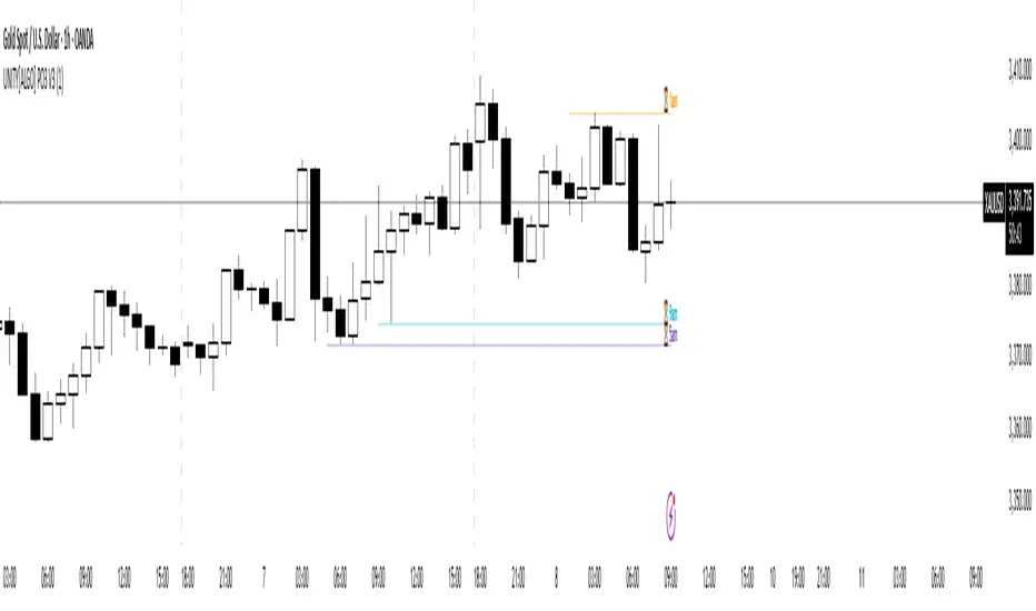
Yellow Candle (High Volume)
Yellow candles indicate High Volume.
Triggered when:
Current candle volume >= Average volume of last 20 candles × volume multiplier
Default multiplier: 1.5
Confirms strong breakouts. Not a standalone entry signal.
---
Head & Shoulders Detection
Supports:
Head & Shoulders (Bearish)
Inverse Head & Shoulders (Bullish)
Neckline drawn automatically. Breakout validated with volume. Pattern status shown in Dashboard.
---
Dashboard
Displays:
Entry Mode (Aggressive / Conservative)
HTF Trend
Current Pattern
Head & Shoulders Status
Market Status: ENTRY BUY, ENTRY SELL, WAIT RETEST, SCANNING
---
Alerts
Alerts trigger only when:
Pattern confirmed
Breakout / Retest logic satisfied
High volume confirmed
Trend filter (if enabled) passes
No trade labels plotted on chart.
---
License & Attribution
Licensed under Creative Commons Attribution 4.0 (CC BY 4.0)
Free to use and modify. Attribution required. Removing or changing the author name is not allowed.
---
This indicator is for technical analysis purposes only and is not financial advice. Always use proper risk management.
---
Clean chart, smart analysis, better trading decisions.
Penunjuk Pine Script®