MIDAS VWAP Jayy his is just a bash together of two MIDAS VWAP scripts particularly AkifTokuz and drshoe.
I added the ability to show more MIDAS curves from the same script.
The algorithm primarily uses the "n" number but the date can be used for the 8th VWAP
I have not converted the script to version 3.
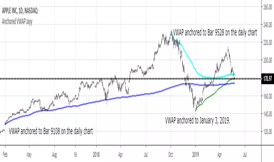
To find bar number go into "Chart Properties" select " "background" then select Indicator Titles and "Indicator values". When you place your cursor over a bar the first number you see adjacent to the script title is the bar number. Put that in the dialogue box midline is MIDAS VWAP . The resistance is a MIDAS VWAP using bar highs. The resistance is MIDAS VWAP using bar lows.
In most case using N will suffice. However, if you are flipping around charts inputting a specific date can be handy. In this way, you can compare the same point in time across multiple instruments eg first trading day of the year or an election date.
Adding dates into the dialogue box is a bit cumbersome so in this version, it is enabled for only one curve. I have called it VWAP and it follows the typical VWAP algorithm. (Does that make a difference? Read below re my opinion on the Difference between MIDAS VWAP and VWAP ).
I have added the ability to start from the bottom or top of the initiating bar.
In theory in a probable uptrend pick a low of a bar for a low pivot and start the MIDAS VWAP there using the support.
For a downtrend use the high pivot bar and select resistance. The way to see is to play with these values.
Difference between MIDAS VWAP and the regular VWAP
MIDAS itself as described by Levine uses a time anchored On-Balance Volume (OBV) plotted on a graph where the horizontal (abscissa) arm of the graph is cumulative volume not time. He called his VWAP curves Support/Resistance VWAP or S/R curves. These S/R curves are often referred to as "MIDAS curves".
These are the main components of the MIDAS chart. A third algorithm called the Top-Bottom Finder was also described. (Separate script).
Additional tools have been described in "MIDAS_Technical_Analysis"
Midas Technical Analysis: A VWAP Approach to Trading and Investing in Today’s Markets by Andrew Coles, David G. Hawkins
Copyright © 2011 by Andrew Coles and David G. Hawkins.
Denoting the different way in which Levine approached the calculation.
The difference between "MIDAS" VWAP and VWAP is, in my opinion, much ado about nothing. The algorithms generate identical curves albeit the MIDAS algorithm launches the curve one bar later than the VWAP algorithm which can be a pain in the neck. All of the algorithms that I looked at on Tradingview step back one bar in time to initiate the MIDAS curve. As such the plotted curves are identical to traditional VWAP assuming the initiation is from the candle/bar midpoint.
How did Levine intend the curves to be drawn?
On a reversal, he suggested the initiation of the Support and Resistance VVWAP (S/R curve) to be started after a reversal.
It is clear in his examples this happens occasionally but in many cases he initiates the so-called MIDAS S/R VWAP right at the reversal point. In any case, the algorithm is problematic if you wish to start a curve on the first bar of an IPO .
You will get nothing. That is a pain. Also in Levine's writings, he describes simply clicking on the point where a
S/R VWAP is to be drawn from. As such, the generally accepted method of initiating the curve at N-1 is a practical and sensible method. The only issue is that you cannot draw the curve from the first bar on any security, as mentioned without resorting to the typical VWAP algorithm. There is another difference. VWAP is launched from the middle of the bar (as per AlphaTrends), You can also launch from the top of the bar or the bottom (or anywhere for that matter). The calculation proceeds using the top or bottom for each new bar.
The potential applications are discussed in the MIDAS Technical Analysis book.
Penunjuk Pine Script®