Smart MACD Divergence ScannerOriginal Base Indicator: "CM_MacD_Ult_MTF" by ChrisMoody
This indicator builds upon ChrisMoody's excellent multi-timeframe MACD foundation and transforms it into a professional divergence scanner with advanced quality assessment and filtering capabilities. The original MACD visualization and MTF functionality have been preserved while adding completely new divergence detection, scoring, and filtering systems.
🎯 What Makes This Indicator Unique:
Smart MACD Divergence Scanner is a professional tool for detecting MACD-based divergences with an advanced filtering system and signal quality assessment. Unlike standard divergence indicators, this version includes innovative features:
Adaptive Quality Scoring System — each signal receives a score from 0 to 100 based on multiple factors
Volatility Filter — automatic signal suppression during low market volatility periods
Multi-Timeframe Confirmation — divergence verification on higher timeframe for increased reliability
Divergence Strength Analysis — calculation of percentage difference between price and indicator movement
Information Dashboard — detailed real-time signal statistics
Cooldown System — prevention of multiple consecutive signals
💡 How It Works:
The indicator uses the classic divergence concept — the divergence between price movement and the MACD oscillator. However, instead of simple pivot detection, the algorithm:
Scans the market for local extremes (pivots) on price and MACD histogram
Searches for divergences — when price updates low/high while MACD shows opposite movement
Assesses quality — analyzes divergence strength, volatility, higher timeframe confirmation
Filters noise — eliminates weak signals through threshold system and cooldown
Generates signal — only when all quality criteria are met
🔧 Key Parameters:
MACD Settings: Fast Length (12), Slow Length (26), Signal Length (9)
Divergence Detection: Pivot Lookback (5), Max Lookback Range (60), Min Divergence Strength (15%)
Quality Filters: Min Quality Score (60), Volatility Filter, MTF Confirmation, Signal Cooldown (5)
📊 How to Use:
Add indicator to chart — it will automatically start scanning
Configure filters — start with default settings, then adapt to your trading style
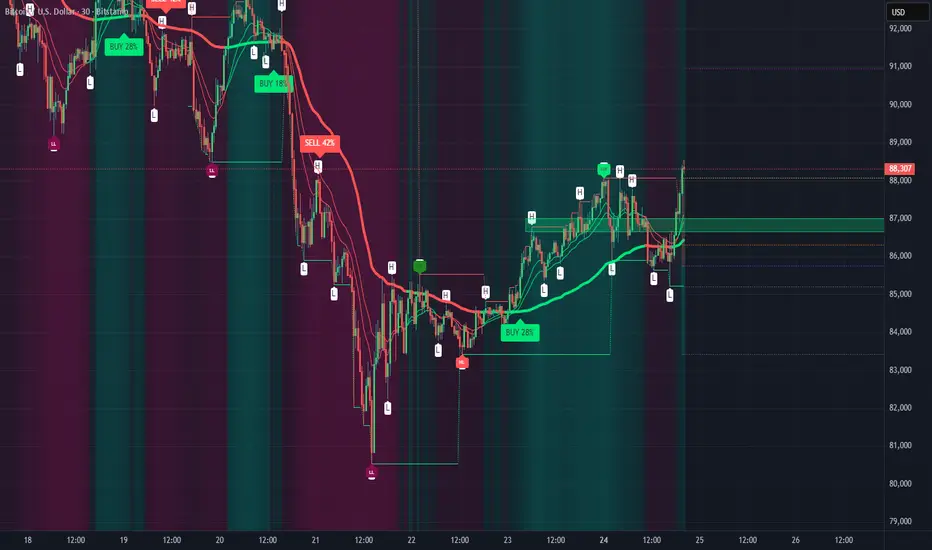
Watch for signals: 🟢 Green "BUY" label = bullish divergence, 🔴 Red "SELL" label = bearish divergence
Check quality score on labels (Q: XX)
Use information panel to monitor statistics and current market conditions
⚙️ Settings Guide:
For swing trading (4H-Daily): Increase Pivot Lookback to 7-10, set Min Quality Score to 70+
For day trading (15m-1H): Keep default settings, enable all filters
For scalping (1m-5m): Decrease Min Quality Score to 50, disable MTF Confirmation
For volatile markets (crypto): Increase Min Divergence Strength to 20-25%, enable Volatility Filter
⚠️ Important Notes:
Divergences are probabilistic signals, not guaranteed reversals
Use additional confirmation (support/resistance levels, volume, price action)
Adjust parameters for specific asset and timeframe
Signals appear with Pivot Lookback bars delay (retrospective confirmation)
On volatile markets, increase Min Quality Score to reduce false signals
Penunjuk Pine Script®