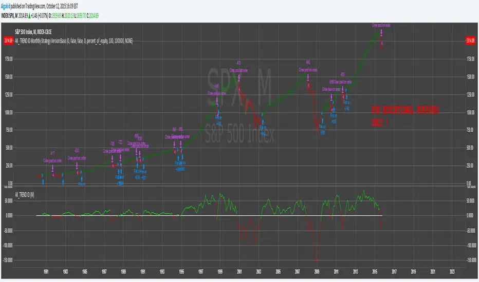
AK_ TREND ID AS A STRATEGY : FOR EDUCATIONAL PURPOSES ONLYJust converted the AK_ TREND ID into a strategy , to show the efficiency of this simple indicator. I used SPX in this example, to display that the indicator has been accurate for a long time.
Cari dalam skrip untuk "algo"
Guided144Algorithm conditions suggested by a friend, works best on daily tf for bitcoin.
simple cycle trading of buy and sell..
A great guide for trading those complicated moves.


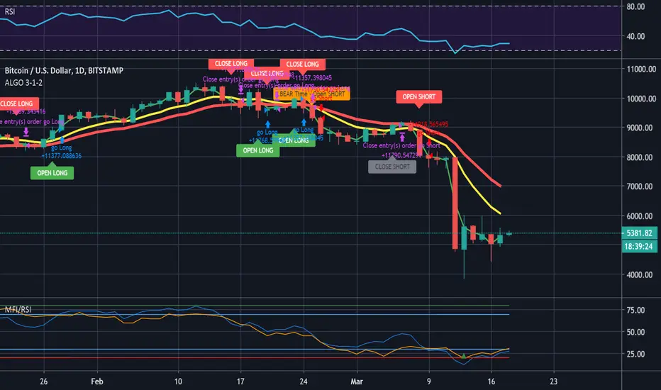
ALGO 3h, 1h, 2hThis script tracks the crossing of the 10EMA on the 3h timeframe and the 200EMA on the 1h timeframe to open LONGS and SHORTS. Whether those LONGS or SHORTS actually trigger is based on the first 2 EMA's position in relation to a 3rd "controller" EMA.

11// This Pine Script® code is subject to the terms of the Mozilla Public License 2.0 at mozilla.org
// © gilanns
//@version=5
//
VERSION = 'v13'// 2024.3.20
strategy(
'ALGOX',
shorttitle = 'ALGOX ' + VERSION,
overlay = true,
explicit_plot_zorder = true,
pyramiding = 0,
default_qty_type = strategy.percent_of_equity,
default_qty_value = 50,
calc_on_every_tick = false,
process_orders_on_close = true,
max_bars_back = 500,
initial_capital = 5000,
commission_type = strategy.commission.percent,
commission_value = 0.02
)
//Truncate Function
truncate(number, decimals) =>
factor = math.pow(10, decimals)
int(number * factor) / factor
//
// === INPUTS ===
TPSType = input.string('Trailing', 'What TPS should be taken : ', options = )
setupType = input.string('Open/Close', title='What Trading Setup should be taken : ', options= )
scolor = input(true, title='Show coloured Bars to indicate Trend?')
almaRibbon = input(false, title='Enable Ribbon?')
//tradeType = input.string('BOTH', title='What trades should be taken : ', options= )
// === /INPUTS ===
// Display the probabilities in a table
//text01_ = str.tostring(timeframe.multiplier * intRes, '####')
//t = timenow + math.round(ta.change(time) * 25)
//var label lab01 = na
//label.delete(lab01)
//lab01 := label.new(t, close, text=text01_, style=label.style_label_left, yloc=yloc.price, xloc=xloc.bar_time, textalign=text.align_left, textcolor=color.white)
// Constants colours that include fully non-transparent option.
green100 = #008000FF
lime100 = #00FF00FF
red100 = #FF0000FF
blue100 = #0000FFFF
aqua100 = #00FFFFFF
darkred100 = #8B0000FF
gray100 = #808080FF
/////////////////////////////////////////////
// Create non-repainting security function
rp_security(_symbol, _res, _src) =>
request.security(_symbol, _res, _src )
//
f_tfInMinutes() =>
_tfInMinutes = timeframe.period == '1' ? '3' : timeframe.period == '3' ? '5' : timeframe.period == '5' ? '15' : timeframe.period == '15' ? '30' : timeframe.period == '30' ? '60' : timeframe.period == '60' ? '240' : 'D'
_tfInMinutes
my_time1 = f_tfInMinutes()
tfmult = 18 //input.int(18, "Input Timeframe Multiplier")
f_resInMinutes() =>
_resInMinutes = timeframe.multiplier * (
timeframe.isseconds ? 1. / 60. :
timeframe.isminutes ? 1. :
timeframe.isdaily ? 1440. :
timeframe.isweekly ? 10080. :
timeframe.ismonthly ? 43800. : na)
my_time = str.tostring(f_resInMinutes()*tfmult)
useSource = close //input.string('Close', 'What Source to be used?', options = )
enableFilter = input(true, "Enable Backtesting Range Filtering")
fromDate = input.time(timestamp("01 Jan 2023 00:00 +0300"), "Start Date")
toDate = input.time(timestamp("31 Dec 2099 00:00 +0300"), "End Date")
tradeDateIsAllowed = not enableFilter or (time >= fromDate and time <= toDate)
filter1 = 'Filter with Atr'
filter2 = 'Filter with RSI'
filter3 = 'Atr or RSI'
filter4 = 'Atr and RSI'
filter5 = 'No Filtering'
filter6 = 'Entry Only in sideways market(By ATR or RSI)'
filter7 = 'Entry Only in sideways market(By ATR and RSI)'
typefilter = input.string(filter5, title='Sideways Filtering Input', options= , group='Strategy Options')
RSI = truncate(ta.rsi(close, input.int(7, group='RSI Filterring')), 2)
toplimitrsi = input.int(45, title='TOP Limit', group='RSI Filterring')
botlimitrsi = input.int(10, title='BOT Limit', group='RSI Filterring')
//ST = input.bool(true, title='Show Supertrend?', group='Supertrend Indicator')
//period = input.int(1440, group='Supertrend Indicator')
//mult = input.float(2.612, group='Supertrend Indicator')
atrfiltLen = 5 //input.int(5, minval=1, title='atr Length', group='Sideways Filtering Input')
atrMaType = 'EMA' //input.string('EMA', options= , group='Sideways Filtering Input', title='atr Moving Average Type')
atrMaLen = 5 //input.int(5, minval=1, title='atr MA Length', group='Sideways Filtering Input')
//filtering
atra = request.security(syminfo.tickerid, '', ta.atr(atrfiltLen))
atrMa = atrMaType == 'EM' ? ta.ema(atra, atrMaLen) : ta.sma(atra, atrMaLen)
updm = ta.change(high)
downdm = -ta.change(low)
plusdm = na(updm) ? na : updm > downdm and updm > 0 ? updm : 0
minusdm = na(downdm) ? na : downdm > updm and downdm > 0 ? downdm : 0
cndSidwayss1 = atra >= atrMa
cndSidwayss2 = RSI > toplimitrsi or RSI < botlimitrsi
cndSidways = cndSidwayss1 or cndSidwayss2
cndSidways1 = cndSidwayss1 and cndSidwayss2
Sidwayss1 = atra <= atrMa
Sidwayss2 = RSI < toplimitrsi and RSI > botlimitrsi
Sidways = Sidwayss1 or Sidwayss2
Sidways1 = Sidwayss1 and Sidwayss2
trendType = typefilter == filter1 ? cndSidwayss1 : typefilter == filter2 ? cndSidwayss2 : typefilter == filter3 ? cndSidways : typefilter == filter4 ? cndSidways1 : typefilter == filter5 ? RSI > 0 : typefilter == filter6 ? Sidways : typefilter == filter7 ? Sidways1 : na
// === /INPUTS ===
tf = my_time //input('15')
r = ticker.heikinashi(syminfo.tickerid)
openSeriesAlt = request.security(r, tf, open, lookahead=barmerge.lookahead_on)
closeSeriesAlt = request.security(r, tf, close, lookahead=barmerge.lookahead_on)
//openP = plot(almaRibbon ? openSeriesAlt : na, color=color.new(color.lime, 0), linewidth=3)
//closeP = plot(almaRibbon ? closeSeriesAlt : na, color=color.new(color.red, 0), linewidth=3)
BUYOC = ta.crossover(closeSeriesAlt, openSeriesAlt) and setupType == "Open/Close" and trendType
SELLOC = ta.crossunder(closeSeriesAlt, openSeriesAlt) and setupType == "Open/Close" and trendType
//strategy.entry('sell', direction=strategy.short, qty=trade_size, comment='sell', when=sel_entry)
//strategy.entry('buy', direction=strategy.long, qty=trade_size, comment='buy', when=buy_entry)
//trendColour = closeSeriesAlt > openSeriesAlt ? color.green : color.red
//bcolour = closeSeriesAlt > openSeriesAlt ? lime100 : red100
//barcolor(scolor ? bcolour : na, title='Bar Colours')
//closeP = plot(almaRibbon ? closeSeriesAlt : na, title='Close Series', color=color.new(trendColour, 20), linewidth=2, style=plot.style_line)
//openP = plot(almaRibbon ? openSeriesAlt : na, title='Open Series', color=color.new(trendColour, 20), linewidth=2, style=plot.style_line)
//fill(closeP, openP, color=color.new(trendColour, 80))
//
//rt = input(true, title="ATR Based REnko is the Default, UnCheck to use Traditional ATR?")
atrLen = 3 //input.int(3, title="RENKO_ATR", group = "Renko Settings")
isATR = true //input.bool(true, title="RENKO_USE_RENKO_ATR", group = "Renko Settings")
tradLen1 = 1000 //input.int(1000, title="RENKO_TRADITIONAL", group = "Renko Settings")
//Code to be implemented in V2
//mul = input(1, "Number Of minticks")
//value = mul * syminfo.mintick
tradLen = tradLen1 * 1
param = isATR ? ticker.renko(syminfo.tickerid, "ATR", atrLen) : ticker.renko(syminfo.tickerid, "Traditional", tradLen)
renko_close = request.security(param, my_time, close, lookahead=barmerge.lookahead_on)
renko_open = request.security(param, my_time, open, lookahead=barmerge.lookahead_on)
//============================================
//Sniper------------------------------------------------------------------------------------------------------------------------------------- // Signal 2
//============================================
//============================================
//EMA_CROSS-------------------------------------------------------------------------------------------------------------------------------- // Signal 4
//============================================
EMA1_length=input.int(2, "EMA1_length", group = "Renko Settings")
EMA2_length=input.int(10, "EMA2_length", group = "Renko Settings")
a = ta.ema(renko_close, EMA1_length)
b = ta.ema(renko_close, EMA2_length)
//BUY = ta.cross(a, b) and a > b and renko_open < renko_close
//SELL = ta.cross(a, b) and a < b and renko_close < renko_open
///////////////////////////////
// Determine long and short conditions
BUYR = ta.crossover(a, b) and setupType == "Renko" and trendType
SELLR = ta.crossunder(a, b) and setupType == "Renko" and trendType
sel_color = setupType == "Open/Close" ? closeSeriesAlt < openSeriesAlt : setupType == "Renko" ? renko_close < renko_open : na
buy_color = setupType == "Open/Close" ? closeSeriesAlt > openSeriesAlt : setupType == "Renko" ? renko_close > renko_open : na
sel_entry = setupType == "Open/Close" ? SELLOC : setupType == "Renko" ? SELLR : na
buy_entry = setupType == "Open/Close" ? BUYOC : setupType == "Renko" ? BUYR : na
trendColour = buy_color ? color.green : color.red
bcolour = buy_color ? lime100 : red100
barcolor(scolor ? bcolour : na, title='Bar Colours')
p11=plot(almaRibbon and setupType == "Open/Close" ? closeSeriesAlt : almaRibbon and setupType == "Renko" ? renko_close : na, style=plot.style_circles, linewidth=1, color=color.new(trendColour, 80), title="RENKO_1")
p22=plot(almaRibbon and setupType == "Open/Close" ? openSeriesAlt : almaRibbon and setupType == "Renko" ? renko_open : na, style=plot.style_circles, linewidth=1, color=color.new(trendColour, 80), title="RENKO_2")
fill(p11, p22, color=color.new(trendColour, 50), title="RENKO_fill")
//
lxTrigger = false
sxTrigger = false
leTrigger = buy_entry
seTrigger = sel_entry
// === /ALERT conditions.
buy = leTrigger //ta.crossover(closeSeriesAlt, openSeriesAlt)
sell = seTrigger //ta.crossunder(closeSeriesAlt, openSeriesAlt)
varip wasLong = false
varip wasShort = false
if barstate.isconfirmed
wasLong := false
else
if buy
wasLong := true
if barstate.isconfirmed
wasShort := false
else
if sell
wasShort := true
plotshape(wasLong, color = color.yellow)
plotshape(wasShort, color = color.yellow)
//plotshape(almaRibbon ? buy : na, title = "Buy", text = 'Buy', style = shape.labelup, location = location.belowbar, color= #39ff14, textcolor = #FFFFFF, size = size.tiny)
//plotshape(almaRibbon ? sell : na, title = "Exit", text = 'Exit', style = shape.labeldown, location = location.abovebar, color= #ff1100, textcolor = #FFFFFF, size = size.tiny)
// === STRATEGY ===
i_alert_txt_entry_long = "Short Exit" //input.text_area(defval = "Short Exit", title = "Long Entry Message", group = "Alerts")
i_alert_txt_exit_long = "Long Exit" //input.text_area(defval = "Long Exit", title = "Long Exit Message", group = "Alerts")
i_alert_txt_entry_short = "Go Short" //input.text_area(defval = "Go Short", title = "Short Entry Message", group = "Alerts")
i_alert_txt_exit_short = "Go Long" //input.text_area(defval = "Go Long", title = "Short Exit Message", group = "Alerts")
// Entries and Exits with TP/SL
//tradeType
if buy and TPSType == "Trailing" and tradeDateIsAllowed
strategy.close("Short" , alert_message = i_alert_txt_exit_short)
strategy.entry("Long" , strategy.long , alert_message = i_alert_txt_entry_long)
if sell and TPSType == "Trailing" and tradeDateIsAllowed
strategy.close("Long" , alert_message = i_alert_txt_exit_long)
strategy.entry("Short" , strategy.short, alert_message = i_alert_txt_entry_short)
//tradeType
if buy and TPSType == "Options" and tradeDateIsAllowed
// strategy.close("Short" , alert_message = i_alert_txt_exit_short)
strategy.entry("Long" , strategy.long , alert_message = i_alert_txt_entry_long)
if sell and TPSType == "Options" and tradeDateIsAllowed
strategy.close("Long" , alert_message = i_alert_txt_exit_long)
// strategy.entry("Short" , strategy.short, alert_message = i_alert_txt_entry_short)
G_RISK = '■ ' + 'Risk Management'
//#region ———— <↓↓↓ G_RISK ↓↓↓> {
//ATR SL Settings
atrLength = 20 //input.int(20, minval=1, title='ATR Length')
profitFactor = 2.5 //input(2.5, title='Take Profit Factor')
stopFactor = 1 //input(1.0, title='Stop Loss Factor')
// Calculate ATR
tpatrValue = ta.atr(atrLength)
// Calculate take profit and stop loss levels for buy signals
takeProfit1_buy = 1 * profitFactor * tpatrValue //close + profitFactor * atrValue
takeProfit2_buy = 2 * profitFactor * tpatrValue //close + 2 * profitFactor * atrValue
takeProfit3_buy = 3 * profitFactor * tpatrValue //close + 3 * profitFactor * atrValue
stopLoss_buy = close - takeProfit1_buy //stopFactor * tpatrValue
// Calculate take profit and stop loss levels for sell signals
takeProfit1_sell = 1 * profitFactor * tpatrValue //close - profitFactor * atrValue
takeProfit2_sell = 2 * profitFactor * tpatrValue //close - 2 * profitFactor * atrValue
takeProfit3_sell = 3 * profitFactor * tpatrValue //close - 3 * profitFactor * atrValue
stopLoss_sell = close + takeProfit1_sell //stopFactor * tpatrValue
// ———————————
//Tooltip
T_LVL = '(%) Exit Level'
T_QTY = '(%) Adjust trade exit volume'
T_MSG = 'Paste JSON message for your bot'
//Webhook Message
O_LEMSG = 'Long Entry'
O_LXMSGSL = 'Long SL'
O_LXMSGTP1 = 'Long TP1'
O_LXMSGTP2 = 'Long TP2'
O_LXMSGTP3 = 'Long TP3'
O_LXMSG = 'Long Exit'
O_SEMSG = 'Short Entry'
O_SXMSGSL = 'Short SL'
O_SXMSGA = 'Short TP1'
O_SXMSGB = 'Short TP2'
O_SXMSGC = 'Short TP3'
O_SXMSGX = 'Short Exit'
// on whole pips) for forex currency pairs.
pip_size = syminfo.mintick * (syminfo.type == "forex" ? 10 : 1)
// On the last historical bar, show the instrument's pip size
//if barstate.islastconfirmedhistory
// label.new(x=bar_index + 2, y=close, style=label.style_label_left,
// color=color.navy, textcolor=color.white, size=size.large,
// text=syminfo.ticker + "'s pip size is:\n" +
// str.tostring(pip_size))
// ——————————— | | | Line length guide |
i_lxLvlTP1 = leTrigger ? takeProfit1_buy : seTrigger ? takeProfit1_sell : na //input.float (1, 'Level TP1' , group = G_RISK, tooltip = T_LVL)
i_lxQtyTP1 = input.float (50, 'Qty TP1' , group = G_RISK, tooltip = T_QTY)
i_lxLvlTP2 = leTrigger ? takeProfit2_buy : seTrigger ? takeProfit2_sell : na //input.float (1.5, 'Level TP2' , group = G_RISK, tooltip = T_LVL)
i_lxQtyTP2 = input.float (30, 'Qty TP2' , group = G_RISK, tooltip = T_QTY)
i_lxLvlTP3 = leTrigger ? takeProfit3_buy : seTrigger ? takeProfit3_sell : na //input.float (2, 'Level TP3' , group = G_RISK, tooltip = T_LVL)
i_lxQtyTP3 = input.float (20, 'Qty TP3' , group = G_RISK, tooltip = T_QTY)
i_lxLvlSL = leTrigger ? takeProfit1_buy : seTrigger ? takeProfit1_sell : na //input.float (0.5, 'Stop Loss' , group = G_RISK, tooltip = T_LVL)
i_sxLvlTP1 = i_lxLvlTP1
i_sxQtyTP1 = i_lxQtyTP1
i_sxLvlTP2 = i_lxLvlTP2
i_sxQtyTP2 = i_lxQtyTP2
i_sxLvlTP3 = i_lxLvlTP3
i_sxQtyTP3 = i_lxQtyTP3
i_sxLvlSL = i_lxLvlSL
G_MSG = '■ ' + 'Webhook Message'
i_leMsg = O_LEMSG //input.string (O_LEMSG ,'Long Entry' , group = G_MSG, tooltip = T_MSG)
i_lxMsgSL = O_LXMSGSL //input.string (O_LXMSGSL ,'Long SL' , group = G_MSG, tooltip = T_MSG)
i_lxMsgTP1 = O_LXMSGTP1 //input.string (O_LXMSGTP1,'Long TP1' , group = G_MSG, tooltip = T_MSG)
i_lxMsgTP2 = O_LXMSGTP2 //input.string (O_LXMSGTP2,'Long TP2' , group = G_MSG, tooltip = T_MSG)
i_lxMsgTP3 = O_LXMSGTP3 //input.string (O_LXMSGTP3,'Long TP3' , group = G_MSG, tooltip = T_MSG)
i_lxMsg = O_LXMSG //input.string (O_LXMSG ,'Long Exit' , group = G_MSG, tooltip = T_MSG)
i_seMsg = O_SEMSG //input.string (O_SEMSG ,'Short Entry' , group = G_MSG, tooltip = T_MSG)
i_sxMsgSL = O_SXMSGSL //input.string (O_SXMSGSL ,'Short SL' , group = G_MSG, tooltip = T_MSG)
i_sxMsgTP1 = O_SXMSGA //input.string (O_SXMSGA ,'Short TP1' , group = G_MSG, tooltip = T_MSG)
i_sxMsgTP2 = O_SXMSGB //input.string (O_SXMSGB ,'Short TP2' , group = G_MSG, tooltip = T_MSG)
i_sxMsgTP3 = O_SXMSGC //input.string (O_SXMSGC ,'Short TP3' , group = G_MSG, tooltip = T_MSG)
i_sxMsg = O_SXMSGX //input.string (O_SXMSGX ,'Short Exit' , group = G_MSG, tooltip = T_MSG)
i_src = close
G_DISPLAY = 'Display'
//
i_alertOn = true //input.bool (true, 'Alert Labels On/Off' , group = G_DISPLAY)
i_barColOn = true //input.bool (true, 'Bar Color On/Off' , group = G_DISPLAY)
// ———————————
// @function Calculate the Take Profit line, and the crossover or crossunder
f_tp(_condition, _conditionValue, _leTrigger, _seTrigger, _src, _lxLvlTP, _sxLvlTP)=>
var float _tpLine = 0.0
_topLvl = _src + _lxLvlTP //TPSType == "Fixed %" ? _src + (_src * (_lxLvlTP / 100)) : _src + _lxLvlTP
_botLvl = _src - _lxLvlTP //TPSType == "Fixed %" ? _src - (_src * (_sxLvlTP / 100)) : _src - _sxLvlTP
_tpLine := _condition != _conditionValue and _leTrigger ? _topLvl :
_condition != -_conditionValue and _seTrigger ? _botLvl :
nz(_tpLine )
// @function Similar to "ta.crossover" or "ta.crossunder"
f_cross(_scr1, _scr2, _over)=>
_cross = _over ? _scr1 > _scr2 and _scr1 < _scr2 :
_scr1 < _scr2 and _scr1 > _scr2
// ———————————
//
var float condition = 0.0
var float slLine = 0.0
var float entryLine = 0.0
//
entryLine := leTrigger and condition <= 0.0 ? close :
seTrigger and condition >= 0.0 ? close : nz(entryLine )
//
slTopLvl = TPSType == "Fixed %" ? i_src + (i_src * (i_lxLvlSL / 100)) : i_src + i_lxLvlSL
slBotLvl = TPSType == "Fixed %" ? i_src - (i_src * (i_sxLvlSL / 100)) : i_src - i_lxLvlSL
slLine := condition <= 0.0 and leTrigger ? slBotLvl :
condition >= 0.0 and seTrigger ? slTopLvl : nz(slLine )
slLong = f_cross(low, slLine, false)
slShort = f_cross(high, slLine, true )
//
= f_tp(condition, 1.2,leTrigger, seTrigger, i_src, i_lxLvlTP3, i_sxLvlTP3)
= f_tp(condition, 1.1,leTrigger, seTrigger, i_src, i_lxLvlTP2, i_sxLvlTP2)
= f_tp(condition, 1.0,leTrigger, seTrigger, i_src, i_lxLvlTP1, i_sxLvlTP1)
tp3Long = f_cross(high, tp3Line, true )
tp3Short = f_cross(low, tp3Line, false)
tp2Long = f_cross(high, tp2Line, true )
tp2Short = f_cross(low, tp2Line, false)
tp1Long = f_cross(high, tp1Line, true )
tp1Short = f_cross(low, tp1Line, false)
switch
leTrigger and condition <= 0.0 => condition := 1.0
seTrigger and condition >= 0.0 => condition := -1.0
tp3Long and condition == 1.2 => condition := 1.3
tp3Short and condition == -1.2 => condition := -1.3
tp2Long and condition == 1.1 => condition := 1.2
tp2Short and condition == -1.1 => condition := -1.2
tp1Long and condition == 1.0 => condition := 1.1
tp1Short and condition == -1.0 => condition := -1.1
slLong and condition >= 1.0 => condition := 0.0
slShort and condition <= -1.0 => condition := 0.0
lxTrigger and condition >= 1.0 => condition := 0.0
sxTrigger and condition <= -1.0 => condition := 0.0
longE = leTrigger and condition <= 0.0 and condition == 1.0
shortE = seTrigger and condition >= 0.0 and condition == -1.0
longX = lxTrigger and condition >= 1.0 and condition == 0.0
shortX = sxTrigger and condition <= -1.0 and condition == 0.0
longSL = slLong and condition >= 1.0 and condition == 0.0
shortSL = slShort and condition <= -1.0 and condition == 0.0
longTP3 = tp3Long and condition == 1.2 and condition == 1.3
shortTP3 = tp3Short and condition == -1.2 and condition == -1.3
longTP2 = tp2Long and condition == 1.1 and condition == 1.2
shortTP2 = tp2Short and condition == -1.1 and condition == -1.2
longTP1 = tp1Long and condition == 1.0 and condition == 1.1
shortTP1 = tp1Short and condition == -1.0 and condition == -1.1
// ——————————— {
//
if strategy.position_size <= 0 and longE and TPSType == "ATR" and tradeDateIsAllowed
strategy.entry( 'Long', strategy.long, alert_message = i_leMsg, comment = 'LE')
if strategy.position_size > 0 and condition == 1.0 and TPSType == "ATR" and tradeDateIsAllowed
strategy.exit( id = 'LXTP1', from_entry = 'Long', qty_percent = i_lxQtyTP1, limit = tp1Line, stop = slLine, comment_profit = 'LXTP1', comment_loss = 'SL', alert_profit = i_lxMsgTP1, alert_loss = i_lxMsgSL)
if strategy.position_size > 0 and condition == 1.1 and TPSType == "ATR" and tradeDateIsAllowed
strategy.exit( id = 'LXTP2', from_entry = 'Long', qty_percent = i_lxQtyTP2, limit = tp2Line, stop = slLine, comment_profit = 'LXTP2', comment_loss = 'SL', alert_profit = i_lxMsgTP2, alert_loss = i_lxMsgSL)
if strategy.position_size > 0 and condition == 1.2 and TPSType == "ATR" and tradeDateIsAllowed
strategy.exit( id = 'LXTP3', from_entry = 'Long', qty_percent = i_lxQtyTP3, limit = tp3Line, stop = slLine, comment_profit = 'LXTP3', comment_loss = 'SL', alert_profit = i_lxMsgTP3, alert_loss = i_lxMsgSL)
if longX and tradeDateIsAllowed
strategy.close( 'Long', alert_message = i_lxMsg, comment = 'LX')
//
if strategy.position_size >= 0 and shortE and TPSType == "ATR" and tradeDateIsAllowed
strategy.entry( 'Short', strategy.short, alert_message = i_leMsg, comment = 'SE')
if strategy.position_size < 0 and condition == -1.0 and TPSType == "ATR" and tradeDateIsAllowed
strategy.exit( id = 'SXTP1', from_entry = 'Short', qty_percent = i_sxQtyTP1, limit = tp1Line, stop = slLine, comment_profit = 'SXTP1', comment_loss = 'SL', alert_profit = i_sxMsgTP1, alert_loss = i_sxMsgSL)
if strategy.position_size < 0 and condition == -1.1 and TPSType == "ATR" and tradeDateIsAllowed
strategy.exit( id = 'SXTP2', from_entry = 'Short', qty_percent = i_sxQtyTP2, limit = tp2Line, stop = slLine, comment_profit = 'SXTP2', comment_loss = 'SL', alert_profit = i_sxMsgTP2, alert_loss = i_sxMsgSL)
if strategy.position_size < 0 and condition == -1.2 and TPSType == "ATR" and tradeDateIsAllowed
strategy.exit( id = 'SXTP3', from_entry = 'Short', qty_percent = i_sxQtyTP3, limit = tp3Line, stop = slLine, comment_profit = 'SXTP3', comment_loss = 'SL', alert_profit = i_sxMsgTP3, alert_loss = i_sxMsgSL)
if shortX and tradeDateIsAllowed
strategy.close( 'Short', alert_message = i_sxMsg, comment = 'SX')
// ———————————
c_tp = leTrigger or seTrigger ? na :
condition == 0.0 ? na : color.green
c_entry = leTrigger or seTrigger ? na :
condition == 0.0 ? na : color.blue
c_sl = leTrigger or seTrigger ? na :
condition == 0.0 ? na : color.red
p_tp1Line = plot ( condition == 1.0 or condition == -1.0 ? tp1Line : na, title = "TP Line 1", color = c_tp, linewidth = 1, style = plot.style_linebr)
p_tp2Line = plot ( condition == 1.0 or condition == -1.0 or condition == 1.1 or condition == -1.1 ? tp2Line : na, title = "TP Line 2", color = c_tp, linewidth = 1, style = plot.style_linebr)
p_tp3Line = plot ( condition == 1.0 or condition == -1.0 or condition == 1.1 or condition == -1.1 or condition == 1.2 or condition == -1.2 ? tp3Line : na, title = "TP Line 3", color = c_tp, linewidth = 1, style = plot.style_linebr)
p_entryLine = plot ( condition >= 1.0 or condition <= -1.0 ? entryLine : na, title = "Entry Line", color = c_entry, linewidth = 1, style = plot.style_linebr)
p_slLine = plot ( condition == 1.0 or condition == -1.0 or condition == 1.1 or condition == -1.1 or condition == 1.2 or condition == -1.2 ? slLine : na, title = "SL Line", color = c_sl, linewidth = 1, style = plot.style_linebr)
//fill( p_tp3Line, p_entryLine, color = leTrigger or seTrigger ? na :color.new(color.green, 90))
fill( p_entryLine, p_slLine, color = leTrigger or seTrigger ? na :color.new(color.red, 90))
//
plotshape( i_alertOn and longE, title = 'Long', text = 'Long', textcolor = color.white, color = color.green, style = shape.labelup, size = size.tiny, location = location.belowbar)
plotshape( i_alertOn and shortE, title = 'Short', text = 'Short', textcolor = color.white, color = color.red, style = shape.labeldown, size = size.tiny, location = location.abovebar)
plotshape( i_alertOn and (longX or shortX) ? close : na, title = 'Close', text = 'Close', textcolor = color.white, color = color.gray, style = shape.labelup, size = size.tiny, location = location.absolute)
l_tp = i_alertOn and (longTP1 or shortTP1) ? close : na
plotshape( l_tp, title = "TP1 Cross", text = "TP1", textcolor = color.white, color = color.olive, style = shape.labelup, size = size.tiny, location = location.absolute)
plotshape( i_alertOn and (longTP2 or shortTP2) ? close : na, title = "TP2 Cross", text = "TP2", textcolor = color.white, color = color.olive, style = shape.labelup, size = size.tiny, location = location.absolute)
plotshape( i_alertOn and (longTP3 or shortTP3) ? close : na, title = "TP3 Cross", text = "TP3", textcolor = color.white, color = color.olive, style = shape.labelup, size = size.tiny, location = location.absolute)
plotshape( i_alertOn and (longSL or shortSL) ? close : na, title = "SL Cross", text = "SL", textcolor = color.white, color = color.maroon, style = shape.labelup, size = size.tiny, location = location.absolute)
//
plot( na, title = "─── ───", editable = false, display = display.data_window)
plot( condition, title = "condition", editable = false, display = display.data_window)
plot( strategy.position_size * 100, title = ".position_size", editable = false, display = display.data_window)
//#endregion }
// ——————————— <↑↑↑ G_RISK ↑↑↑>
//#region ———— <↓↓↓ G_SCRIPT02 ↓↓↓> {
// @function Queues a new element in an array and de-queues its first element.
f_qDq(_array, _val) =>
array.push(_array, _val)
_return = array.shift(_array)
_return
var line a_slLine = array.new_line(1)
var line a_entryLine = array.new_line(1)
var line a_tp3Line = array.new_line(1)
var line a_tp2Line = array.new_line(1)
var line a_tp1Line = array.new_line(1)
var label a_slLabel = array.new_label(1)
var label a_tp3label = array.new_label(1)
var label a_tp2label = array.new_label(1)
var label a_tp1label = array.new_label(1)
var label a_entryLabel = array.new_label(1)
newEntry = longE or shortE
entryIndex = 1
entryIndex := newEntry ? bar_index : nz(entryIndex )
lasTrade = bar_index >= entryIndex
l_right = 10
if TPSType == "ATR"
line.delete( f_qDq(a_slLine, line.new( entryIndex, slLine, last_bar_index + l_right, slLine, style = line.style_solid, color = c_sl)))
if TPSType == "ATR"
line.delete( f_qDq(a_entryLine, line.new( entryIndex, entryLine, last_bar_index + l_right, entryLine, style = line.style_solid, color = color.blue)))
if TPSType == "ATR"
line.delete( f_qDq(a_tp3Line, line.new( entryIndex, tp3Line, last_bar_index + l_right, tp3Line, style = line.style_solid, color = c_tp)))
if TPSType == "ATR"
line.delete( f_qDq(a_tp2Line, line.new( entryIndex, tp2Line, last_bar_index + l_right, tp2Line, style = line.style_solid, color = c_tp)))
if TPSType == "ATR"
line.delete( f_qDq(a_tp1Line, line.new( entryIndex, tp1Line, last_bar_index + l_right, tp1Line, style = line.style_solid, color = c_tp)))
if TPSType == "ATR"
label.delete( f_qDq(a_slLabel, label.new( last_bar_index + l_right, slLine, 'SL: ' + str.tostring(slLine, '##.###'), style = label.style_label_left, textcolor = color.white, color = c_sl)))
if TPSType == "ATR"
label.delete( f_qDq(a_entryLabel, label.new( last_bar_index + l_right, entryLine, 'Entry: ' + str.tostring(entryLine, '##.###'), style = label.style_label_left, textcolor = color.white, color = color.blue)))
if TPSType == "ATR"
label.delete( f_qDq(a_tp3label, label.new( last_bar_index + l_right, tp3Line, 'TP3: ' + str.tostring(tp3Line, '##.###') + " - Target Pips : - " + str.tostring(longE ? tp3Line - entryLine : entryLine - tp3Line, "#.##"), style = label.style_label_left, textcolor = color.white, color = c_tp)))
if TPSType == "ATR"
label.delete( f_qDq(a_tp2label, label.new( last_bar_index + l_right, tp2Line, 'TP2: ' + str.tostring(tp2Line, '##.###'), style = label.style_label_left, textcolor = color.white, color = c_tp)))
if TPSType == "ATR"
label.delete( f_qDq(a_tp1label, label.new( last_bar_index + l_right, tp1Line, 'TP1: ' + str.tostring(tp1Line, '##.###'), style = label.style_label_left, textcolor = color.white, color = c_tp)))
//#endregion }
// ——————————— <↑↑↑ G_SCRIPT02 ↑↑↑>
c_barCol = close > open ? color.rgb(120, 9, 139) : color.rgb(69, 155, 225)
barcolor(
i_barColOn ? c_barCol : na)
// ———————————
//
if longE or shortE or longX or shortX
alert(message = 'Any Alert', freq = alert.freq_once_per_bar_close)
if longE
alert(message = 'Long Entry', freq = alert.freq_once_per_bar_close)
if shortE
alert(message = 'Short Entry', freq = alert.freq_once_per_bar_close)
if longX
alert(message = 'Long Exit', freq = alert.freq_once_per_bar_close)
if shortX
alert(message = 'Short Exit', freq = alert.freq_once_per_bar_close)
//#endregion }
// ——————————— <↑↑↑ G_SCRIPT03 ↑↑↑>
// This source code is subject to the terms of the Mozilla Public License 2.0 at mozilla.org
// © TraderHalai
// This script was born out of my quest to be able to display strategy back test statistics on charts to allow for easier backtesting on devices that do not natively support backtest engine (such as mobile phones, when I am backtesting from away from my computer). There are already a few good ones on TradingView, but most / many are too complicated for my needs.
//
//Found an excellent display backtest engine by 'The Art of Trading'. This script is a snippet of his hard work, with some very minor tweaks and changes. Much respect to the original author.
//
//Full credit to the original author of this script. It can be found here: www.tradingview.com
//
// This script can be copied and airlifted onto existing strategy scripts of your own, and integrates out of the box without implementation of additional functions. I've also added Max Runup, Average Win and Average Loss per trade to the orignal script.
//
//Will look to add in more performance metrics in future, as I further develop this script.
//
//Feel free to use this display panel in your scripts and strategies.
//Thanks and enjoy! :)
//@version=5
//strategy("Strategy BackTest Display Statistics - TraderHalai", overlay=true, default_qty_value= 5, default_qty_type = strategy.percent_of_equity, initial_capital=10000, commission_type=strategy.commission.percent, commission_value=0.1)
//DEMO basic strategy - Use your own strategy here - Jaws Mean Reversion from my profile used here
//source = input(title = "Source", defval = close)
///////////////////////////// --- BEGIN TESTER CODE --- ////////////////////////
// COPY below into your strategy to enable display
////////////////////////////////////////////////////////////////////////////////
// Declare performance tracking variables
drawTester = input.bool(true, "Strategy Performance", group='Dashboards', inline="Show Dashboards")
var balance = strategy.initial_capital
var drawdown = 0.0
var maxDrawdown = 0.0
var maxBalance = 0.0
var totalWins = 0
var totalLoss = 0
// Prepare stats table
var table testTable = table.new(position.top_right, 5, 2, border_width=1)
f_fillCell(_table, _column, _row, _title, _value, _bgcolor, _txtcolor) =>
_cellText = _title + "\n" + _value
table.cell(_table, _column, _row, _cellText, bgcolor=_bgcolor, text_color=_txtcolor)
// Custom function to truncate (cut) excess decimal places
//truncate(_number, _decimalPlaces) =>
// _factor = math.pow(10, _decimalPlaces)
// int(_number * _factor) / _factor
// Draw stats table
var bgcolor = color.new(color.black,0)
if drawTester and tradeDateIsAllowed
if barstate.islastconfirmedhistory
// Update table
dollarReturn = strategy.netprofit
f_fillCell(testTable, 0, 0, "Total Trades:", str.tostring(strategy.closedtrades), bgcolor, color.white)
f_fillCell(testTable, 0, 1, "Win Rate:", str.tostring(truncate((strategy.wintrades/strategy.closedtrades)*100,2)) + "%", bgcolor, color.white)
f_fillCell(testTable, 1, 0, "Starting:", "$" + str.tostring(strategy.initial_capital), bgcolor, color.white)
f_fillCell(testTable, 1, 1, "Ending:", "$" + str.tostring(truncate(strategy.initial_capital + strategy.netprofit,2)), bgcolor, color.white)
f_fillCell(testTable, 2, 0, "Avg Win:", "$"+ str.tostring(truncate(strategy.grossprofit / strategy.wintrades, 2)), bgcolor, color.white)
f_fillCell(testTable, 2, 1, "Avg Loss:", "$"+ str.tostring(truncate(strategy.grossloss / strategy.losstrades, 2)), bgcolor, color.white)
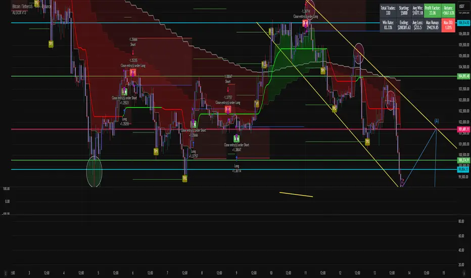
f_fillCell(testTable, 3, 0, "Profit Factor:", str.tostring(truncate(strategy.grossprofit / strategy.grossloss,2)), strategy.grossprofit > strategy.grossloss ? color.green : color.red, color.white)
f_fillCell(testTable, 3, 1, "Max Runup:", str.tostring(truncate(strategy.max_runup, 2 )), bgcolor, color.white)
f_fillCell(testTable, 4, 0, "Return:", (dollarReturn > 0 ? "+" : "") + str.tostring(truncate((dollarReturn / strategy.initial_capital)*100,2)) + "%", dollarReturn > 0 ? color.green : color.red, color.white)
f_fillCell(testTable, 4, 1, "Max DD:", str.tostring(truncate((strategy.max_drawdown / strategy.equity) * 100 ,2)) + "%", color.red, color.white)
// --- END TESTER CODE --- ///////////////
// This Pine Script™ code is subject to the terms of the Mozilla Public License 2.0 at mozilla.org
// © niceGear68734
//@version=5
//strategy("Table to filter trades per day", overlay=true, use_bar_magnifier = true, initial_capital = 5000, calc_on_every_tick = true, calc_on_order_fills = true, commission_type = strategy.commission.cash_per_contract)
//~ ___________________________________________________________________________
//~ !!!!!!!!!!!!!!!!!!!!!!!!!!!!!!!!!!!!!!!!!!!!!!!!!!!!!!!!!!!!!!!!!!!!!!!!!!!
//~ !!!!!!!!!!!!!!!_________________ START _________________!!!!!!!!!!!!!!!!!
i_showweeklyPerformance = input.bool(false, 'Weekly Performance', group='Dashboards', inline="Show Dashboards")
//__________________________ User Inputs ___________________________________
var const string g_table = "Table Settings"
i_table_pos = "Top Left" //input.string(defval = "Top Left", title = "Position", options = , group = g_table, inline = "1", tooltip = "It sets the location of the table")
i_text_size = "Normal" //input.string(defval = "Normal", title = "Set the size of text", options = , tooltip = "This option is used to change the size of the text in the table")
var const string g_general = "General Settings"
i_check_open_close = "Opened" //input.string("Opened", "Check when the trade :", , group = g_general, tooltip = "This parameter defines what to check for. If opened is selected, the results will show the trades that opened on that day. If closed is selected, the results will show the trades that closed on that day")
i_timezone = "Exchange" //input.string("Exchange", title = "Set the Timezone", options = , group = g_general, tooltip = "You can use this setting whenever you want to change the time that the trade has closed/opened")
//~_____________________________ Switches ___________________________________
table_pos = switch i_table_pos
"Bottom Right" => position.bottom_right
"Bottom Left" => position.bottom_left
"Top Right" => position.top_right
"Top Left" => position.top_left
timezone_setting = i_timezone == "Exchange" ? syminfo.timezone : i_timezone
text_size = switch i_text_size
"Small" => size.small
"Normal" => size.normal
"Large" => size.large
//__________________________ Array Declaration _____________________________
var string t_column_names = array.from( "", "Sun", "Mon", "Tue", "Wed", "Thur", "Fri", "Sat") // Columns header names
var string t_row_names = array.from("", "Total Trades", "Loss", "Win", "Win Rate" ) // Rows header names
var t_column_size = array.size(t_column_names)
var t_row_size = array.size(t_row_names)
var string a_closed_trades = array.new_string() // Save the total number of trades
var string a_loss_trades = array.new_string() // Save the number of losing trades
var string a_win_trades = array.new_string() // Save the number of winning trades
var _a_day_week = array.new_int() // Save the day of the week to split data
// __________________________ Custom Functions ________________________________
//~ create a counter so that it gives a number to strategy.closed_trades.entry_time(counter)
var trade_number = -1
if strategy.closedtrades > strategy.closedtrades
trade_number += 1
f_strategy_closedtrades_hour() =>
switch
i_check_open_close =="Closed" => dayofweek(strategy.closedtrades.exit_time(trade_number), timezone_setting)
i_check_open_close =="Opened" => dayofweek(strategy.closedtrades.entry_time(trade_number), timezone_setting)
f_data(_i) =>
var _closed_trades = 0
var _loss_trades = 0
var _win_trades = 0
var _txt_closed_trades = ""
var _txt_loss_trades = ""
var _txt_win_trades = ""
if strategy.closedtrades > strategy.closedtrades and f_strategy_closedtrades_hour() == _i
_closed_trades += 1
_txt_closed_trades := str.tostring(_closed_trades)
if strategy.losstrades > strategy.losstrades and f_strategy_closedtrades_hour() == _i
_loss_trades += 1
_txt_loss_trades := str.tostring(_loss_trades)
if strategy.wintrades > strategy.wintrades and f_strategy_closedtrades_hour() == _i
_win_trades += 1
_txt_win_trades := str.tostring(_win_trades)
//__________________________
var string array1 = array.new_string(5)
var string array2 = array.new_string(5)
var string array3 = array.new_string(5)
var string array4 = array.new_string(5)
var string array5 = array.new_string(5)
var string array6 = array.new_string(5)
var string array7 = array.new_string(5)
f_pass_data_to_array(_i, _array) =>
= f_data(_i)
array.set(_array,1 , cl)
array.set(_array,2,loss)
array.set(_array,3,win)
if cl != ""
array.set(_array,4,str.tostring(str.tonumber(win) / str.tonumber(cl) * 100 , "##") + " %")
if cl != "" and win == ""
array.set(_array,4,"0 %")
for i = 1 to 7
switch
i == 1 => f_pass_data_to_array(i,array1)
i == 2 => f_pass_data_to_array(i,array2)
i == 3 => f_pass_data_to_array(i,array3)
i == 4 => f_pass_data_to_array(i,array4)
i == 5 => f_pass_data_to_array(i,array5)
i == 6 => f_pass_data_to_array(i,array6)
i == 7 => f_pass_data_to_array(i,array7)
f_retrieve_data_to_table(_i, _j) =>
switch
_i == 1 => array.get(array1, _j)
_i == 2 => array.get(array2, _j)
_i == 3 => array.get(array3, _j)
_i == 4 => array.get(array4, _j)
_i == 5 => array.get(array5, _j)
_i == 6 => array.get(array6, _j)
_i == 7 => array.get(array7, _j)
//~ ___________________________ Create Table ________________________________
create_table(_col, _row, _txt) =>
var table _tbl = table.new(position = table_pos, columns = t_column_size , rows = t_row_size, border_width=1)
color _color = _row == 0 or _col == 0 ? color.rgb(3, 62, 106) : color.rgb(2, 81, 155)
table.cell(_tbl, _col, _row, _txt, bgcolor = _color, text_color = color.white, text_size = text_size)
//~___________________________ Fill With Data _______________________________
if barstate.islastconfirmedhistory and i_showweeklyPerformance and tradeDateIsAllowed
for i = 0 to t_column_size - 1 by 1
for j = 0 to t_row_size - 1 by 1
_txt = ""
if i >= 0 and j == 0
_txt := array.get(t_column_names, i)
if j >= 0 and i == 0
_txt := array.get(t_row_names, j)
if i >= 1 and j >= 1 and j <= 5
_txt := f_retrieve_data_to_table( i , j)
create_table(i ,j , _txt)
//~ ___________________________ Notice ______________________________________
if timeframe.in_seconds() > timeframe.in_seconds("D")
x = table.new(position.middle_center,1,1,color.aqua)
table.cell_set_text(x,0,0,"Please select lower timeframes (Daily or lower)")
//~ !!!!!!!!!!!!!!!_________________ STOP _________________!!!!!!!!!!!!!!!!!!
//~ !!!!!!!!!!!!!!!!!!!!!!!!!!!!!!!!!!!!!!!!!!!!!!!!!!!!!!!!!!!!!!!!!!!!!!!!!!!
//~ ___________________________________________________________________________
// Global Dashboard Variables
// ░░░░░░░░░░░░░░░░░░░░░░░░░░░░░░░░░░░░░░░░░░░░░░░░░░░░░░░░░░░░░░░░░░░░░░░░░░░░░░░░░░░░░░░░░░░░░░░░░░░░░░░░░░░░░░░░░░░░░░░░░░░░░░░░░░░░░░░░░░░░░░░░░░
// Dashboard Table Text Size
i_tableTextSize = "Normal" //input.string(title="Dashboard Size", defval="Normal", options= , group="Dashboards")
table_text_size(s) =>
switch s
"Auto" => size.auto
"Huge" => size.huge
"Large" => size.large
"Normal" => size.normal
"Small" => size.small
=> size.tiny
tableTextSize = table_text_size(i_tableTextSize)
// Monthly Table Performance Dashboard By @QuantNomad
// ░░░░░░░░░░░░░░░░░░░░░░░░░░░░░░░░░░░░░░░░░░░░░░░░░░░░░░░░░░░░░░░░░░░░░░░░░░░░░░░░░░░░░░░░░░░░░░░░░░░░░░░░░░░░░░░░░░░░░░░░░░░░░░░░░░░░░░░░░░░░░░░░░░
i_showMonthlyPerformance = input.bool(false, 'Monthly Performance', group='Dashboards', inline="Show Dashboards")
i_monthlyReturnPercision = 2
if i_showMonthlyPerformance and tradeDateIsAllowed
new_month = month(time) != month(time )
new_year = year(time) != year(time )
eq = strategy.equity
bar_pnl = eq / eq - 1
cur_month_pnl = 0.0
cur_year_pnl = 0.0
// Current Monthly P&L;
cur_month_pnl := new_month ? 0.0 :
(1 + cur_month_pnl ) * (1 + bar_pnl) - 1
// Current Yearly P&L;
cur_year_pnl := new_year ? 0.0 :
(1 + cur_year_pnl ) * (1 + bar_pnl) - 1
// Arrays to store Yearly and Monthly P&Ls;
var month_pnl = array.new_float(0)
var month_time = array.new_int(0)
var year_pnl = array.new_float(0)
var year_time = array.new_int(0)
last_computed = false
if (not na(cur_month_pnl ) and (new_month or barstate.islastconfirmedhistory))
if (last_computed )
array.pop(month_pnl)
array.pop(month_time)
array.push(month_pnl , cur_month_pnl )
array.push(month_time, time )
if (not na(cur_year_pnl ) and (new_year or barstate.islastconfirmedhistory))
if (last_computed )
array.pop(year_pnl)
array.pop(year_time)
array.push(year_pnl , cur_year_pnl )
array.push(year_time, time )
last_computed := barstate.islastconfirmedhistory ? true : nz(last_computed )
// Monthly P&L; Table
var monthly_table = table(na)
if (barstate.islastconfirmedhistory)
monthly_table := table.new(position.bottom_right, columns = 14, rows = array.size(year_pnl) + 1, border_width = 1)
table.cell(monthly_table, 0, 0, "", bgcolor = #cccccc, text_size=tableTextSize)
table.cell(monthly_table, 1, 0, "Jan", bgcolor = #cccccc, text_size=tableTextSize)
table.cell(monthly_table, 2, 0, "Feb", bgcolor = #cccccc, text_size=tableTextSize)
table.cell(monthly_table, 3, 0, "Mar", bgcolor = #cccccc, text_size=tableTextSize)
table.cell(monthly_table, 4, 0, "Apr", bgcolor = #cccccc, text_size=tableTextSize)
table.cell(monthly_table, 5, 0, "May", bgcolor = #cccccc, text_size=tableTextSize)
table.cell(monthly_table, 6, 0, "Jun", bgcolor = #cccccc, text_size=tableTextSize)
table.cell(monthly_table, 7, 0, "Jul", bgcolor = #cccccc, text_size=tableTextSize)
table.cell(monthly_table, 8, 0, "Aug", bgcolor = #cccccc, text_size=tableTextSize)
table.cell(monthly_table, 9, 0, "Sep", bgcolor = #cccccc, text_size=tableTextSize)
table.cell(monthly_table, 10, 0, "Oct", bgcolor = #cccccc, text_size=tableTextSize)
table.cell(monthly_table, 11, 0, "Nov", bgcolor = #cccccc, text_size=tableTextSize)
table.cell(monthly_table, 12, 0, "Dec", bgcolor = #cccccc, text_size=tableTextSize)
table.cell(monthly_table, 13, 0, "Year", bgcolor = #999999, text_size=tableTextSize)
for yi = 0 to array.size(year_pnl) - 1
table.cell(monthly_table, 0, yi + 1, str.tostring(year(array.get(year_time, yi))), bgcolor = #cccccc, text_size=tableTextSize)
y_color = array.get(year_pnl, yi) > 0 ? color.new(color.teal, transp = 40) : color.new(color.gray, transp = 40)
table.cell(monthly_table, 13, yi + 1, str.tostring(math.round(array.get(year_pnl, yi) * 100, i_monthlyReturnPercision)), bgcolor = y_color, text_color=color.new(color.white, 0),text_size=tableTextSize)
for mi = 0 to array.size(month_time) - 1
m_row = year(array.get(month_time, mi)) - year(array.get(year_time, 0)) + 1
m_col = month(array.get(month_time, mi))
m_color = array.get(month_pnl, mi) > 0 ? color.new(color.teal, transp = 40) : color.new(color.maroon, transp = 40)
table.cell(monthly_table, m_col, m_row, str.tostring(math.round(array.get(month_pnl, mi) * 100, i_monthlyReturnPercision)), bgcolor = m_color, text_color=color.new(color.white, 0), text_size=tableTextSize)
hide = timeframe.isintraday
// Input for EMA period
emaPeriod = 48 //input.int(48, title="EMA Period")
emaPeriod2 = 2 //input.int(2, title="EME Period 2")
emaPeriod3 = 21 //input.int(21, title="EMA Period")
// Input to toggle EMA Cloud
showcloud = input.bool(true, title="Plot EMA?", group='EMA & ATR', inline="Show EMA's & ATR")
useHTF = input.bool(true, title = "Use Higher Time Frame?")
matimeframe = useHTF ? my_time1 : ''
// EMA calculations
ema = request.security(syminfo.tickerid, matimeframe, ta.ema(close, emaPeriod))
ema2 = request.security(syminfo.tickerid, matimeframe, ta.ema(close,emaPeriod2))
ema3 = request.security(syminfo.tickerid, matimeframe,ta.ema(close, emaPeriod3))
emaColor = close > ema3 ? color.new(color.rgb(56, 142, 60, 63), 50) : color.new(color.rgb(147, 40, 51, 38), 50)
// Plotting EMA's
plot_ema1 = plot(hide ? ema : na, style=plot.style_line, color=color.new(color.rgb(255, 255, 255, 100), 50), title="EMA", linewidth=2)
plot_ema2 = plot(hide ? ema2 : na, style=plot.style_line, color=color.new(color.rgb(255, 255, 255, 100), 50), title="EMA", linewidth=1)
plot_ema3 = plot(ema3, style=plot.style_line, color=emaColor, title="EMA", linewidth=1)
// EMA Cloud
cloudColor = ema2 > ema ? color.new(#0f8513, 80) : color.new(#a81414, 80)
cloudColor2 = ema2 > ema3 ? color.new(#0f8513, 50) : color.new(#a81414, 50)
cloudColor := showcloud ? cloudColor : na
fill(plot_ema1, plot_ema2, color=cloudColor, title="EMA Cloud")
fill(plot_ema3, plot_ema2, color=cloudColor, title="EMA Cloud")
/////////////////////////////////////////////////////////////// © BackQuant ///////////////////////////////////////////////////////////////
// This Pine Script™ code is subject to the terms of the Mozilla Public License 2.0 at mozilla.org
// © BackQuant
import TradingView/ta/4 as ta
//@version=5
//indicator(
// title="DEMA Adjusted Average True Range ",
// shorttitle = "DEMA ATR ",
// overlay=true,
// timeframe="",
// timeframe_gaps=true
// )
// Define User Inputs
simple bool showAtr = input.bool(true, "Plot Dema?", group='EMA & ATR', inline="Show EMA's & ATR")
simple bool haCandles = true //input.bool(true, "Use HA Candles?")
simple int periodDema = 7 //input.int(7, "Dema Period", group = "Dema Atr")
series float sourceDema = close //input.source(close, "Calculation Source", group = "Dema Atr")
simple int periodAtr = 14 //input.int(14, "Period", group = "Dema Atr")
simple float factorAtr = 1.7 //input.float(1.7, "Factor", step = 0.01, group = "Dema Atr")
simple color longColour = #00ff00
simple color shortColour = #ff0000
/////////////////////////////////////////////////////////////// © BackQuant ///////////////////////////////////////////////////////////////
// Use HA Candles?
heikinashi_close = request.security(
symbol = ticker.heikinashi(syminfo.tickerid),
timeframe = timeframe.period,
expression = close,
gaps = barmerge.gaps_off,
lookahead = barmerge.lookahead_on
)
var series float source = close
if haCandles == true
source := heikinashi_close
if haCandles == false
source := sourceDema
/////////////////////////////////////////////////////////////// © BackQuant ///////////////////////////////////////////////////////////////
// Function
DemaAtrWithBands(periodDema, source, lookback, atrFactor)=>
ema1 = ta.ema(source, periodDema)
ema2 = ta.ema(ema1, periodDema)
demaOut = 2 * ema1 - ema2
atr = ta.atr(lookback)
trueRange = atr * atrFactor
DemaAtr = demaOut
DemaAtr := nz(DemaAtr , DemaAtr)
trueRangeUpper = demaOut + trueRange
trueRangeLower = demaOut - trueRange
if trueRangeLower > DemaAtr
DemaAtr := trueRangeLower
if trueRangeUpper < DemaAtr
DemaAtr := trueRangeUpper
DemaAtr
// Function Out
DemaAtr = DemaAtrWithBands(periodDema, source, periodAtr, factorAtr)
/////////////////////////////////////////////////////////////// © BackQuant ///////////////////////////////////////////////////////////////
// Conditions
DemaAtrLong = DemaAtr > DemaAtr
DemaAtrShort = DemaAtr < DemaAtr
// Colour Condtions
var color Trendcolor = #ffffff
if DemaAtrLong
Trendcolor := longColour
if DemaAtrShort
Trendcolor := shortColour
// Plotting
plot( showAtr ? DemaAtr : na, "ATR", color=Trendcolor, linewidth = 2 )
// ==========================================================================================
[STRATEGY] Moving Average CrossoverHello friends,
This is a comprehensive backtesting engine for Moving Average crossover strategies, supporting over 63 types of moving averages and filters. It allows you to test, compare, and optimize crossover behaviors between any two moving averages with flexible profit and risk management tools.
Built upon the Moving Average Crossover foundation, this advanced version lets you manually backtest more than 4096 combinations of moving average types. When combined with customizable periods, take-profits, and stop-loss levels, the total number of possible configurations becomes virtually unlimited.
🛠 How It Works
The system tests crossovers between two selected moving averages, with full control over their types, lengths, and trading direction. Integrated bracket settings enable dynamic take-profit, stop-loss, and trailing-stop management using units such as % , ATR , points , pips , or ticks .
You can restrict backtesting to a custom date range for focused performance evaluation or run it across the instrument’s full history.
🔥 Key Features
Supports 63+ moving average and filter types — including algorithms by Ehlers , Jurik , Kaufman , Apirine , Tillson , and Dürschner
Customizable MA types, periods, and strategy direction
Full-featured bracket control: TP, SL, and TSL in ATR, %, points, pips, or ticks
Backtest window customization (start, end, or range)
Direction filter: Longs only, Shorts only, or Both
Dynamic trade labeling and color-coded visualization
Option to exit only at TP, SL, or TSL
If you'd like access or have any questions, feel free to reach out to me directly via DM.
👋 Good luck and happy trading!
Paid script

GKD-BT Baseline Backtest [Loxx]The Giga Kaleidoscope GKD-BT Baseline Backtest is a backtesting module included in Loxx's "Giga Kaleidoscope Modularized Trading System."
█ GKD-BT Baseline Backtest
The GKD-BT Baseline Backtest allows traders to backtest the Regular and Stepped baselines used in the GKD trading system. This module includes 65+ moving averages and 15+ types of volatility to choose from.
Additionally, this backtest module provides the option to test the GKD-B indicator with 1 to 3 take profits and 1 stop loss. The Trading backtest allows for the use of 1 to 3 take profits, while the Full backtest is limited to 1 take profit. The Trading backtest also offers the capability to apply a trailing take profit.
In terms of the percentage of trade removed at each take profit, this backtest module has the following hardcoded values:
Take profit 1: 50% of the trade is removed
Take profit 2: 25% of the trade is removed
Take profit 3: 25% of the trade is removed
Stop loss: 100% of the trade is removed
After each take profit is achieved, the stop loss level is adjusted. When take profit 1 is reached, the stop loss is moved to the entry point. Similarly, when take profit 2 is reached, the stop loss is shifted to take profit 1. The trailing take profit feature comes into play after take profit 2 or take profit 3, depending on the number of take profits selected in the settings. The trailing take profit is always activated on the final take profit when 2 or more take profits are chosen.
The backtest also offers the capability to restrict by a specific date range, allowing for simulated forward testing based on past data. Additionally, users have the option to display or hide a trading panel that provides relevant information about the backtest, statistics, and the current trade. It is also possible to activate alerts and toggle sections of the trading panel on or off. On the chart, historical take profit and stop loss levels are represented by horizontal lines overlaid for reference.
This backtest also includes an optional GKD-E Exit indicator that can be used to test early exits.
The GKD system utilizes volatility-based take profits and stop losses. Each take profit and stop loss is calculated as a multiple of volatility. You can change the values of the multipliers in the settings as well.
To utilize this strategy, follow these steps:
1. (Required) Import the value "Input into NEW GKD-BT Backtest" from the GKD-B Baseline indicator into the GKD-BT Baseline Backtest field "Import GKD-B Baseline"
2. (Optional) Import the value "Input into NEW GKD-BT Backtest" from the GKD-E Exit indicator into the GKD-BT Baseline Backtest field "Import GKD-E Exit". You can toggle the Exit on or off using the "Activate GKD-E Exit" option.
Baselines that are compatible with this backtest module:
GKD-B Baseline
GKD-B Stepped Baseline
Volatility Types Included
17 types of volatility are included in this indicator
Close-to-Close
Parkinson
Garman-Klass
Rogers-Satchell
Yang-Zhang
Garman-Klass-Yang-Zhang
Exponential Weighted Moving Average
Standard Deviation of Log Returns
Pseudo GARCH(2,2)
Average True Range
True Range Double
Standard Deviation
Adaptive Deviation
Median Absolute Deviation
Efficiency-Ratio Adaptive ATR
Mean Absolute Deviation
Static Percent
█ Giga Kaleidoscope Modularized Trading System
Core components of an NNFX algorithmic trading strategy
The NNFX algorithm is built on the principles of trend, momentum, and volatility. There are six core components in the NNFX trading algorithm:
1. Volatility - price volatility; e.g., Average True Range, True Range Double, Close-to-Close, etc.
2. Baseline - a moving average to identify price trend
3. Confirmation 1 - a technical indicator used to identify trends
4. Confirmation 2 - a technical indicator used to identify trends
5. Continuation - a technical indicator used to identify trends
6. Volatility/Volume - a technical indicator used to identify volatility/volume breakouts/breakdown
7. Exit - a technical indicator used to determine when a trend is exhausted
8. Metamorphosis - a technical indicator that produces a compound signal from the combination of other GKD indicators*
*(not part of the NNFX algorithm)
What is Volatility in the NNFX trading system?
In the NNFX (No Nonsense Forex) trading system, ATR (Average True Range) is typically used to measure the volatility of an asset. It is used as a part of the system to help determine the appropriate stop loss and take profit levels for a trade. ATR is calculated by taking the average of the true range values over a specified period.
True range is calculated as the maximum of the following values:
-Current high minus the current low
-Absolute value of the current high minus the previous close
-Absolute value of the current low minus the previous close
ATR is a dynamic indicator that changes with changes in volatility. As volatility increases, the value of ATR increases, and as volatility decreases, the value of ATR decreases. By using ATR in NNFX system, traders can adjust their stop loss and take profit levels according to the volatility of the asset being traded. This helps to ensure that the trade is given enough room to move, while also minimizing potential losses.
Other types of volatility include True Range Double (TRD), Close-to-Close, and Garman-Klass
What is a Baseline indicator?
The baseline is essentially a moving average, and is used to determine the overall direction of the market.
The baseline in the NNFX system is used to filter out trades that are not in line with the long-term trend of the market. The baseline is plotted on the chart along with other indicators, such as the Moving Average (MA), the Relative Strength Index (RSI), and the Average True Range (ATR).
Trades are only taken when the price is in the same direction as the baseline. For example, if the baseline is sloping upwards, only long trades are taken, and if the baseline is sloping downwards, only short trades are taken. This approach helps to ensure that trades are in line with the overall trend of the market, and reduces the risk of entering trades that are likely to fail.
By using a baseline in the NNFX system, traders can have a clear reference point for determining the overall trend of the market, and can make more informed trading decisions. The baseline helps to filter out noise and false signals, and ensures that trades are taken in the direction of the long-term trend.
What is a Confirmation indicator?
Confirmation indicators are technical indicators that are used to confirm the signals generated by primary indicators. Primary indicators are the core indicators used in the NNFX system, such as the Average True Range (ATR), the Moving Average (MA), and the Relative Strength Index (RSI).
The purpose of the confirmation indicators is to reduce false signals and improve the accuracy of the trading system. They are designed to confirm the signals generated by the primary indicators by providing additional information about the strength and direction of the trend.
Some examples of confirmation indicators that may be used in the NNFX system include the Bollinger Bands, the MACD (Moving Average Convergence Divergence), and the MACD Oscillator. These indicators can provide information about the volatility, momentum, and trend strength of the market, and can be used to confirm the signals generated by the primary indicators.
In the NNFX system, confirmation indicators are used in combination with primary indicators and other filters to create a trading system that is robust and reliable. By using multiple indicators to confirm trading signals, the system aims to reduce the risk of false signals and improve the overall profitability of the trades.
What is a Continuation indicator?
In the NNFX (No Nonsense Forex) trading system, a continuation indicator is a technical indicator that is used to confirm a current trend and predict that the trend is likely to continue in the same direction. A continuation indicator is typically used in conjunction with other indicators in the system, such as a baseline indicator, to provide a comprehensive trading strategy.
What is a Volatility/Volume indicator?
Volume indicators, such as the On Balance Volume (OBV), the Chaikin Money Flow (CMF), or the Volume Price Trend (VPT), are used to measure the amount of buying and selling activity in a market. They are based on the trading volume of the market, and can provide information about the strength of the trend. In the NNFX system, volume indicators are used to confirm trading signals generated by the Moving Average and the Relative Strength Index. Volatility indicators include Average Direction Index, Waddah Attar, and Volatility Ratio. In the NNFX trading system, volatility is a proxy for volume and vice versa.
By using volume indicators as confirmation tools, the NNFX trading system aims to reduce the risk of false signals and improve the overall profitability of trades. These indicators can provide additional information about the market that is not captured by the primary indicators, and can help traders to make more informed trading decisions. In addition, volume indicators can be used to identify potential changes in market trends and to confirm the strength of price movements.
What is an Exit indicator?
The exit indicator is used in conjunction with other indicators in the system, such as the Moving Average (MA), the Relative Strength Index (RSI), and the Average True Range (ATR), to provide a comprehensive trading strategy.
The exit indicator in the NNFX system can be any technical indicator that is deemed effective at identifying optimal exit points. Examples of exit indicators that are commonly used include the Parabolic SAR, the Average Directional Index (ADX), and the Chandelier Exit.
The purpose of the exit indicator is to identify when a trend is likely to reverse or when the market conditions have changed, signaling the need to exit a trade. By using an exit indicator, traders can manage their risk and prevent significant losses.
In the NNFX system, the exit indicator is used in conjunction with a stop loss and a take profit order to maximize profits and minimize losses. The stop loss order is used to limit the amount of loss that can be incurred if the trade goes against the trader, while the take profit order is used to lock in profits when the trade is moving in the trader's favor.
Overall, the use of an exit indicator in the NNFX trading system is an important component of a comprehensive trading strategy. It allows traders to manage their risk effectively and improve the profitability of their trades by exiting at the right time.
What is an Metamorphosis indicator?
The concept of a metamorphosis indicator involves the integration of two or more GKD indicators to generate a compound signal. This is achieved by evaluating the accuracy of each indicator and selecting the signal from the indicator with the highest accuracy. As an illustration, let's consider a scenario where we calculate the accuracy of 10 indicators and choose the signal from the indicator that demonstrates the highest accuracy.
The resulting output from the metamorphosis indicator can then be utilized in a GKD-BT backtest by occupying a slot that aligns with the purpose of the metamorphosis indicator. The slot can be a GKD-B, GKD-C, or GKD-E slot, depending on the specific requirements and objectives of the indicator. This allows for seamless integration and utilization of the compound signal within the GKD-BT framework.
How does Loxx's GKD (Giga Kaleidoscope Modularized Trading System) implement the NNFX algorithm outlined above?
Loxx's GKD v2.0 system has five types of modules (indicators/strategies). These modules are:
1. GKD-BT - Backtesting module (Volatility, Number 1 in the NNFX algorithm)
2. GKD-B - Baseline module (Baseline and Volatility/Volume, Numbers 1 and 2 in the NNFX algorithm)
3. GKD-C - Confirmation 1/2 and Continuation module (Confirmation 1/2 and Continuation, Numbers 3, 4, and 5 in the NNFX algorithm)
4. GKD-V - Volatility/Volume module (Confirmation 1/2, Number 6 in the NNFX algorithm)
5. GKD-E - Exit module (Exit, Number 7 in the NNFX algorithm)
6. GKD-M - Metamorphosis module (Metamorphosis, Number 8 in the NNFX algorithm, but not part of the NNFX algorithm)
(additional module types will added in future releases)
Each module interacts with every module by passing data to A backtest module wherein the various components of the GKD system are combined to create a trading signal.
That is, the Baseline indicator passes its data to Volatility/Volume. The Volatility/Volume indicator passes its values to the Confirmation 1 indicator. The Confirmation 1 indicator passes its values to the Confirmation 2 indicator. The Confirmation 2 indicator passes its values to the Continuation indicator. The Continuation indicator passes its values to the Exit indicator, and finally, the Exit indicator passes its values to the Backtest strategy.
This chaining of indicators requires that each module conform to Loxx's GKD protocol, therefore allowing for the testing of every possible combination of technical indicators that make up the six components of the NNFX algorithm.
What does the application of the GKD trading system look like?
Example trading system:
Backtest: GKD-BT Baseline Backtest as shown on the chart above
Baseline: Hull Moving Average as shown on the chart above
Volatility/Volume: Hurst Exponent
Confirmation 1: Sherif's HiLo
Confirmation 2: uf2018
Continuation: Coppock Curve
Exit: Fisher Transform as shown on the chart above
Metamorphosis: Baseline Optimizer
Each GKD indicator is denoted with a module identifier of either: GKD-BT, GKD-B, GKD-C, GKD-V, GKD-M, or GKD-E. This allows traders to understand to which module each indicator belongs and where each indicator fits into the GKD system.
█ Giga Kaleidoscope Modularized Trading System Signals
Standard Entry
1. GKD-C Confirmation gives signal
2. Baseline agrees
3. Price inside Goldie Locks Zone Minimum
4. Price inside Goldie Locks Zone Maximum
5. Confirmation 2 agrees
6. Volatility/Volume agrees
1-Candle Standard Entry
1a. GKD-C Confirmation gives signal
2a. Baseline agrees
3a. Price inside Goldie Locks Zone Minimum
4a. Price inside Goldie Locks Zone Maximum
Next Candle
1b. Price retraced
2b. Baseline agrees
3b. Confirmation 1 agrees
4b. Confirmation 2 agrees
5b. Volatility/Volume agrees
Baseline Entry
1. GKD-B Baseline gives signal
2. Confirmation 1 agrees
3. Price inside Goldie Locks Zone Minimum
4. Price inside Goldie Locks Zone Maximum
5. Confirmation 2 agrees
6. Volatility/Volume agrees
7. Confirmation 1 signal was less than 'Maximum Allowable PSBC Bars Back' prior
1-Candle Baseline Entry
1a. GKD-B Baseline gives signal
2a. Confirmation 1 agrees
3a. Price inside Goldie Locks Zone Minimum
4a. Price inside Goldie Locks Zone Maximum
5a. Confirmation 1 signal was less than 'Maximum Allowable PSBC Bars Back' prior
Next Candle
1b. Price retraced
2b. Baseline agrees
3b. Confirmation 1 agrees
4b. Confirmation 2 agrees
5b. Volatility/Volume agrees
Volatility/Volume Entry
1. GKD-V Volatility/Volume gives signal
2. Confirmation 1 agrees
3. Price inside Goldie Locks Zone Minimum
4. Price inside Goldie Locks Zone Maximum
5. Confirmation 2 agrees
6. Baseline agrees
7. Confirmation 1 signal was less than 7 candles prior
1-Candle Volatility/Volume Entry
1a. GKD-V Volatility/Volume gives signal
2a. Confirmation 1 agrees
3a. Price inside Goldie Locks Zone Minimum
4a. Price inside Goldie Locks Zone Maximum
5a. Confirmation 1 signal was less than 'Maximum Allowable PSVVC Bars Back' prior
Next Candle
1b. Price retraced
2b. Volatility/Volume agrees
3b. Confirmation 1 agrees
4b. Confirmation 2 agrees
5b. Baseline agrees
Confirmation 2 Entry
1. GKD-C Confirmation 2 gives signal
2. Confirmation 1 agrees
3. Price inside Goldie Locks Zone Minimum
4. Price inside Goldie Locks Zone Maximum
5. Volatility/Volume agrees
6. Baseline agrees
7. Confirmation 1 signal was less than 7 candles prior
1-Candle Confirmation 2 Entry
1a. GKD-C Confirmation 2 gives signal
2a. Confirmation 1 agrees
3a. Price inside Goldie Locks Zone Minimum
4a. Price inside Goldie Locks Zone Maximum
5a. Confirmation 1 signal was less than 'Maximum Allowable PSC2C Bars Back' prior
Next Candle
1b. Price retraced
2b. Confirmation 2 agrees
3b. Confirmation 1 agrees
4b. Volatility/Volume agrees
5b. Baseline agrees
PullBack Entry
1a. GKD-B Baseline gives signal
2a. Confirmation 1 agrees
3a. Price is beyond 1.0x Volatility of Baseline
Next Candle
1b. Price inside Goldie Locks Zone Minimum
2b. Price inside Goldie Locks Zone Maximum
3b. Confirmation 1 agrees
4b. Confirmation 2 agrees
5b. Volatility/Volume agrees
Continuation Entry
1. Standard Entry, 1-Candle Standard Entry, Baseline Entry, 1-Candle Baseline Entry, Volatility/Volume Entry, 1-Candle Volatility/Volume Entry, Confirmation 2 Entry, 1-Candle Confirmation 2 Entry, or Pullback entry triggered previously
2. Baseline hasn't crossed since entry signal trigger
4. Confirmation 1 agrees
5. Baseline agrees
6. Confirmation 2 agrees
GKD-BT Giga Confirmation Stack Backtest [Loxx]Giga Kaleidoscope GKD-BT Giga Confirmation Stack Backtest is a Backtesting module included in Loxx's "Giga Kaleidoscope Modularized Trading System".
█ GKD-BT Giga Confirmation Stack Backtest
The Giga Confirmation Stack Backtest module allows users to perform backtesting on Long and Short signals from the confluence between GKD-C Confirmation 1 and GKD-C Confirmation 2 indicators. This module encompasses two types of backtests: Trading and Full. The Trading backtest permits users to evaluate individual trades, whether Long or Short, one at a time. Conversely, the Full backtest allows users to analyze either Longs or Shorts separately by toggling between them in the settings, enabling the examination of results for each signal type. The Trading backtest emulates actual trading conditions, while the Full backtest assesses all signals, regardless of being Long or Short.
Additionally, this backtest module provides the option to test using indicators with 1 to 3 take profits and 1 stop loss. The Trading backtest allows for the use of 1 to 3 take profits, while the Full backtest is limited to 1 take profit. The Trading backtest also offers the capability to apply a trailing take profit.
In terms of the percentage of trade removed at each take profit, this backtest module has the following hardcoded values:
Take profit 1: 50% of the trade is removed.
Take profit 2: 25% of the trade is removed.
Take profit 3: 25% of the trade is removed.
Stop loss: 100% of the trade is removed.
After each take profit is achieved, the stop loss level is adjusted. When take profit 1 is reached, the stop loss is moved to the entry point. Similarly, when take profit 2 is reached, the stop loss is shifted to take profit 1. The trailing take profit feature comes into play after take profit 2 or take profit 3, depending on the number of take profits selected in the settings. The trailing take profit is always activated on the final take profit when 2 or more take profits are chosen.
The backtest module also offers the capability to restrict by a specific date range, allowing for simulated forward testing based on past data. Additionally, users have the option to display or hide a trading panel that provides relevant information about the backtest, statistics, and the current trade. It is also possible to activate alerts and toggle sections of the trading panel on or off. On the chart, historical take profit and stop loss levels are represented by horizontal lines overlaid for reference.
To utilize this strategy, follow these steps:
1. Adjust the "Confirmation Type" in the GKD-C Confirmation 1 Indicator to "GKD New."
2. GKD-C Confirmation 1 Import: Import the value "Input into NEW GKD-BT Backtest" from the GKD-C Confirmation 1 module into the GKD-BT Giga Confirmation Stack Backtest module setting named "Import GKD-C Confirmation 1."
3. Adjust the "Confirmation Type" in the GKD-C Confirmation 2 Indicator to "GKD New."
4. GKD-C Confirmation 2 Import: Import the value "Input into NEW GKD-BT Backtest" from the GKD-C Confirmation 2 module into the GKD-BT Giga Confirmation Stack Backtest module setting named "Import GKD-C Confirmation 2."
█ Giga Confirmation Stack Backtest Entries
Entries are generated from the confluence of a GKD-C Confirmation 1 and GKD-C Confirmation 2 indicators. The Confirmation 1 gives the signal and the Confirmation 2 indicator filters or "approves" the the Confirmation 1 signal. If Confirmation 1 gives a long signal and Confirmation 2 shows a downtrend, then the long signal is rejected. If Confirmation 1 gives a long signal and Confirmation 2 shows an uptrend, then the long signal is approved and sent to the backtest execution engine.
█ Volatility Types Included
The GKD system utilizes volatility-based take profits and stop losses. Each take profit and stop loss is calculated as a multiple of volatility. Users can also adjust the multiplier values in the settings.
This module includes 17 types of volatility:
Close-to-Close
Parkinson
Garman-Klass
Rogers-Satchell
Yang-Zhang
Garman-Klass-Yang-Zhang
Exponential Weighted Moving Average
Standard Deviation of Log Returns
Pseudo GARCH(2,2)
Average True Range
True Range Double
Standard Deviation
Adaptive Deviation
Median Absolute Deviation
Efficiency-Ratio Adaptive ATR
Mean Absolute Deviation
Static Percent
Close-to-Close
Close-to-Close volatility is a classic and widely used volatility measure, sometimes referred to as historical volatility.
Volatility is an indicator of the speed of a stock price change. A stock with high volatility is one where the price changes rapidly and with a larger amplitude. The more volatile a stock is, the riskier it is.
Close-to-close historical volatility is calculated using only a stock's closing prices. It is the simplest volatility estimator. However, in many cases, it is not precise enough. Stock prices could jump significantly during a trading session and return to the opening value at the end. That means that a considerable amount of price information is not taken into account by close-to-close volatility.
Despite its drawbacks, Close-to-Close volatility is still useful in cases where the instrument doesn't have intraday prices. For example, mutual funds calculate their net asset values daily or weekly, and thus their prices are not suitable for more sophisticated volatility estimators.
Parkinson
Parkinson volatility is a volatility measure that uses the stock’s high and low price of the day.
The main difference between regular volatility and Parkinson volatility is that the latter uses high and low prices for a day, rather than only the closing price. This is useful as close-to-close prices could show little difference while large price movements could have occurred during the day. Thus, Parkinson's volatility is considered more precise and requires less data for calculation than close-to-close volatility.
One drawback of this estimator is that it doesn't take into account price movements after the market closes. Hence, it systematically undervalues volatility. This drawback is addressed in the Garman-Klass volatility estimator.
Garman-Klass
Garman-Klass is a volatility estimator that incorporates open, low, high, and close prices of a security.
Garman-Klass volatility extends Parkinson's volatility by taking into account the opening and closing prices. As markets are most active during the opening and closing of a trading session, it makes volatility estimation more accurate.
Garman and Klass also assumed that the process of price change follows a continuous diffusion process (Geometric Brownian motion). However, this assumption has several drawbacks. The method is not robust for opening jumps in price and trend movements.
Despite its drawbacks, the Garman-Klass estimator is still more effective than the basic formula since it takes into account not only the price at the beginning and end of the time interval but also intraday price extremes.
Researchers Rogers and Satchell have proposed a more efficient method for assessing historical volatility that takes into account price trends. See Rogers-Satchell Volatility for more detail.
Rogers-Satchell
Rogers-Satchell is an estimator for measuring the volatility of securities with an average return not equal to zero.
Unlike Parkinson and Garman-Klass estimators, Rogers-Satchell incorporates a drift term (mean return not equal to zero). As a result, it provides better volatility estimation when the underlying is trending.
The main disadvantage of this method is that it does not take into account price movements between trading sessions. This leads to an underestimation of volatility since price jumps periodically occur in the market precisely at the moments between sessions.
A more comprehensive estimator that also considers the gaps between sessions was developed based on the Rogers-Satchel formula in the 2000s by Yang-Zhang. See Yang Zhang Volatility for more detail.
Yang-Zhang
Yang Zhang is a historical volatility estimator that handles both opening jumps and the drift and has a minimum estimation error.
Yang-Zhang volatility can be thought of as a combination of the overnight (close-to-open volatility) and a weighted average of the Rogers-Satchell volatility and the day’s open-to-close volatility. It is considered to be 14 times more efficient than the close-to-close estimator.
Garman-Klass-Yang-Zhang
Garman-Klass-Yang-Zhang (GKYZ) volatility estimator incorporates the returns of open, high, low, and closing prices in its calculation.
GKYZ volatility estimator takes into account overnight jumps but not the trend, i.e., it assumes that the underlying asset follows a Geometric Brownian Motion (GBM) process with zero drift. Therefore, the GKYZ volatility estimator tends to overestimate the volatility when the drift is different from zero. However, for a GBM process, this estimator is eight times more efficient than the close-to-close volatility estimator.
Exponential Weighted Moving Average
The Exponentially Weighted Moving Average (EWMA) is a quantitative or statistical measure used to model or describe a time series. The EWMA is widely used in finance, with the main applications being technical analysis and volatility modeling.
The moving average is designed such that older observations are given lower weights. The weights decrease exponentially as the data point gets older – hence the name exponentially weighted.
The only decision a user of the EWMA must make is the parameter lambda. The parameter decides how important the current observation is in the calculation of the EWMA. The higher the value of lambda, the more closely the EWMA tracks the original time series.
Standard Deviation of Log Returns
This is the simplest calculation of volatility. It's the standard deviation of ln(close/close(1)).
Pseudo GARCH(2,2)
This is calculated using a short- and long-run mean of variance multiplied by ?.
?avg(var;M) + (1 ? ?) avg(var;N) = 2?var/(M+1-(M-1)L) + 2(1-?)var/(M+1-(M-1)L)
Solving for ? can be done by minimizing the mean squared error of estimation; that is, regressing L^-1var - avg(var; N) against avg(var; M) - avg(var; N) and using the resulting beta estimate as ?.
Average True Range
The average true range (ATR) is a technical analysis indicator, introduced by market technician J. Welles Wilder Jr. in his book New Concepts in Technical Trading Systems, that measures market volatility by decomposing the entire range of an asset price for that period.
The true range indicator is taken as the greatest of the following: current high less the current low; the absolute value of the current high less the previous close; and the absolute value of the current low less the previous close. The ATR is then a moving average, generally using 14 days, of the true ranges.
True Range Double
A special case of ATR that attempts to correct for volatility skew.
Standard Deviation
Standard deviation is a statistic that measures the dispersion of a dataset relative to its mean and is calculated as the square root of the variance. The standard deviation is calculated as the square root of variance by determining each data point's deviation relative to the mean. If the data points are further from the mean, there is a higher deviation within the data set; thus, the more spread out the data, the higher the standard deviation.
Adaptive Deviation
By definition, the Standard Deviation (STD, also represented by the Greek letter sigma ? or the Latin letter s) is a measure that is used to quantify the amount of variation or dispersion of a set of data values. In technical analysis, we usually use it to measure the level of current volatility.
Standard Deviation is based on Simple Moving Average calculation for mean value. This version of standard deviation uses the properties of EMA to calculate what can be called a new type of deviation, and since it is based on EMA, we can call it EMA deviation. Additionally, Perry Kaufman's efficiency ratio is used to make it adaptive (since all EMA type calculations are nearly perfect for adapting).
The difference when compared to the standard is significant--not just because of EMA usage, but the efficiency ratio makes it a "bit more logical" in very volatile market conditions.
Median Absolute Deviation
The median absolute deviation is a measure of statistical dispersion. Moreover, the MAD is a robust statistic, being more resilient to outliers in a data set than the standard deviation. In the standard deviation, the distances from the mean are squared, so large deviations are weighted more heavily, and thus outliers can heavily influence it. In the MAD, the deviations of a small number of outliers are irrelevant.
Because the MAD is a more robust estimator of scale than the sample variance or standard deviation, it works better with distributions without a mean or variance, such as the Cauchy distribution.
Efficiency-Ratio Adaptive ATR
Average True Range (ATR) is a widely used indicator for many occasions in technical analysis. It is calculated as the RMA of the true range. This version adds a "twist": it uses Perry Kaufman's Efficiency Ratio to calculate adaptive true range.
Mean Absolute Deviation
The mean absolute deviation (MAD) is a measure of variability that indicates the average distance between observations and their mean. MAD uses the original units of the data, which simplifies interpretation. Larger values signify that the data points spread out further from the average. Conversely, lower values correspond to data points bunching closer to it. The mean absolute deviation is also known as the mean deviation and average absolute deviation.
This definition of the mean absolute deviation sounds similar to the standard deviation (SD). While both measure variability, they have different calculations. In recent years, some proponents of MAD have suggested that it replace the SD as the primary measure because it is a simpler concept that better fits real life.
Static Percent
Static Percent allows the user to insert their own constant percent that will then be used to create take profits and stoploss
█ Giga Kaleidoscope Modularized Trading System
Core components of an NNFX algorithmic trading strategy
The NNFX algorithm is built on the principles of trend, momentum, and volatility. There are six core components in the NNFX trading algorithm:
1. Volatility - price volatility; e.g., Average True Range, True Range Double, Close-to-Close, etc.
2. Baseline - a moving average to identify price trend
3. Confirmation 1 - a technical indicator used to identify trends
4. Confirmation 2 - a technical indicator used to identify trends
5. Continuation - a technical indicator used to identify trends
6. Volatility/Volume - a technical indicator used to identify volatility/volume breakouts/breakdown
7. Exit - a technical indicator used to determine when a trend is exhausted
What is Volatility in the NNFX trading system?
In the NNFX (No Nonsense Forex) trading system, ATR (Average True Range) is typically used to measure the volatility of an asset. It is used as a part of the system to help determine the appropriate stop loss and take profit levels for a trade. ATR is calculated by taking the average of the true range values over a specified period.
True range is calculated as the maximum of the following values:
-Current high minus the current low
-Absolute value of the current high minus the previous close
-Absolute value of the current low minus the previous close
ATR is a dynamic indicator that changes with changes in volatility. As volatility increases, the value of ATR increases, and as volatility decreases, the value of ATR decreases. By using ATR in NNFX system, traders can adjust their stop loss and take profit levels according to the volatility of the asset being traded. This helps to ensure that the trade is given enough room to move, while also minimizing potential losses.
Other types of volatility include True Range Double (TRD), Close-to-Close, and Garman-Klass
What is a Baseline indicator?
The baseline is essentially a moving average, and is used to determine the overall direction of the market.
The baseline in the NNFX system is used to filter out trades that are not in line with the long-term trend of the market. The baseline is plotted on the chart along with other indicators, such as the Moving Average (MA), the Relative Strength Index (RSI), and the Average True Range (ATR).
Trades are only taken when the price is in the same direction as the baseline. For example, if the baseline is sloping upwards, only long trades are taken, and if the baseline is sloping downwards, only short trades are taken. This approach helps to ensure that trades are in line with the overall trend of the market, and reduces the risk of entering trades that are likely to fail.
By using a baseline in the NNFX system, traders can have a clear reference point for determining the overall trend of the market, and can make more informed trading decisions. The baseline helps to filter out noise and false signals, and ensures that trades are taken in the direction of the long-term trend.
What is a Confirmation indicator?
Confirmation indicators are technical indicators that are used to confirm the signals generated by primary indicators. Primary indicators are the core indicators used in the NNFX system, such as the Average True Range (ATR), the Moving Average (MA), and the Relative Strength Index (RSI).
The purpose of the confirmation indicators is to reduce false signals and improve the accuracy of the trading system. They are designed to confirm the signals generated by the primary indicators by providing additional information about the strength and direction of the trend.
Some examples of confirmation indicators that may be used in the NNFX system include the Bollinger Bands, the MACD (Moving Average Convergence Divergence), and the MACD Oscillator. These indicators can provide information about the volatility, momentum, and trend strength of the market, and can be used to confirm the signals generated by the primary indicators.
In the NNFX system, confirmation indicators are used in combination with primary indicators and other filters to create a trading system that is robust and reliable. By using multiple indicators to confirm trading signals, the system aims to reduce the risk of false signals and improve the overall profitability of the trades.
What is a Continuation indicator?
In the NNFX (No Nonsense Forex) trading system, a continuation indicator is a technical indicator that is used to confirm a current trend and predict that the trend is likely to continue in the same direction. A continuation indicator is typically used in conjunction with other indicators in the system, such as a baseline indicator, to provide a comprehensive trading strategy.
What is a Volatility/Volume indicator?
Volume indicators, such as the On Balance Volume (OBV), the Chaikin Money Flow (CMF), or the Volume Price Trend (VPT), are used to measure the amount of buying and selling activity in a market. They are based on the trading volume of the market, and can provide information about the strength of the trend. In the NNFX system, volume indicators are used to confirm trading signals generated by the Moving Average and the Relative Strength Index. Volatility indicators include Average Direction Index, Waddah Attar, and Volatility Ratio. In the NNFX trading system, volatility is a proxy for volume and vice versa.
By using volume indicators as confirmation tools, the NNFX trading system aims to reduce the risk of false signals and improve the overall profitability of trades. These indicators can provide additional information about the market that is not captured by the primary indicators, and can help traders to make more informed trading decisions. In addition, volume indicators can be used to identify potential changes in market trends and to confirm the strength of price movements.
What is an Exit indicator?
The exit indicator is used in conjunction with other indicators in the system, such as the Moving Average (MA), the Relative Strength Index (RSI), and the Average True Range (ATR), to provide a comprehensive trading strategy.
The exit indicator in the NNFX system can be any technical indicator that is deemed effective at identifying optimal exit points. Examples of exit indicators that are commonly used include the Parabolic SAR, the Average Directional Index (ADX), and the Chandelier Exit.
The purpose of the exit indicator is to identify when a trend is likely to reverse or when the market conditions have changed, signaling the need to exit a trade. By using an exit indicator, traders can manage their risk and prevent significant losses.
In the NNFX system, the exit indicator is used in conjunction with a stop loss and a take profit order to maximize profits and minimize losses. The stop loss order is used to limit the amount of loss that can be incurred if the trade goes against the trader, while the take profit order is used to lock in profits when the trade is moving in the trader's favor.
Overall, the use of an exit indicator in the NNFX trading system is an important component of a comprehensive trading strategy. It allows traders to manage their risk effectively and improve the profitability of their trades by exiting at the right time.
How does Loxx's GKD (Giga Kaleidoscope Modularized Trading System) implement the NNFX algorithm outlined above?
Loxx's GKD v2.0 system has five types of modules (indicators/strategies). These modules are:
1. GKD-BT - Backtesting module (Volatility, Number 1 in the NNFX algorithm)
2. GKD-B - Baseline module (Baseline and Volatility/Volume, Numbers 1 and 2 in the NNFX algorithm)
3. GKD-C - Confirmation 1/2 and Continuation module (Confirmation 1/2 and Continuation, Numbers 3, 4, and 5 in the NNFX algorithm)
4. GKD-V - Volatility/Volume module (Confirmation 1/2, Number 6 in the NNFX algorithm)
5. GKD-E - Exit module (Exit, Number 7 in the NNFX algorithm)
(additional module types will added in future releases)
Each module interacts with every module by passing data to A backtest module wherein the various components of the GKD system are combined to create a trading signal.
That is, the Baseline indicator passes its data to Volatility/Volume. The Volatility/Volume indicator passes its values to the Confirmation 1 indicator. The Confirmation 1 indicator passes its values to the Confirmation 2 indicator. The Confirmation 2 indicator passes its values to the Continuation indicator. The Continuation indicator passes its values to the Exit indicator, and finally, the Exit indicator passes its values to the Backtest strategy.
This chaining of indicators requires that each module conform to Loxx's GKD protocol, therefore allowing for the testing of every possible combination of technical indicators that make up the six components of the NNFX algorithm.
What does the application of the GKD trading system look like?
Example trading system:
Backtest: Confiramtion Stack Backtest
Baseline: Hull Moving Average
Volatility/Volume: Hurst Exponent
Confirmation 1: Fisher Transform as shown on the chart above
Confirmation 2: uf2018 as shown on the chart above
Continuation: Vortex
Exit: Rex Oscillator
Each GKD indicator is denoted with a module identifier of either: GKD-BT, GKD-B, GKD-C, GKD-V, or GKD-E. This allows traders to understand to which module each indicator belongs and where each indicator fits into the GKD system.
GKD-BT Giga Stacks Backtest [Loxx]Giga Kaleidoscope GKD-BT Giga Stacks Backtest is a Backtesting module included in Loxx's "Giga Kaleidoscope Modularized Trading System".
█ GKD-BT Giga Stacks Backtest
The Giga Stacks Backtest module allows users to perform backtesting on Long and Short signals from the confluence of GKD-B Baseline, GKD-C Confirmation, and GKD-V Volatility/Volume indicators. This module encompasses two types of backtests: Trading and Full. The Trading backtest permits users to evaluate individual trades, whether Long or Short, one at a time. Conversely, the Full backtest allows users to analyze either Longs or Shorts separately by toggling between them in the settings, enabling the examination of results for each signal type. The Trading backtest emulates actual trading conditions, while the Full backtest assesses all signals, regardless of being Long or Short.
Additionally, this backtest module provides the option to test using indicators with 1 to 3 take profits and 1 stop loss. The Trading backtest allows for the use of 1 to 3 take profits, while the Full backtest is limited to 1 take profit. The Trading backtest also offers the capability to apply a trailing take profit.
In terms of the percentage of trade removed at each take profit, this backtest module has the following hardcoded values:
Take profit 1: 50% of the trade is removed.
Take profit 2: 25% of the trade is removed.
Take profit 3: 25% of the trade is removed.
Stop loss: 100% of the trade is removed.
After each take profit is achieved, the stop loss level is adjusted. When take profit 1 is reached, the stop loss is moved to the entry point. Similarly, when take profit 2 is reached, the stop loss is shifted to take profit 1. The trailing take profit feature comes into play after take profit 2 or take profit 3, depending on the number of take profits selected in the settings. The trailing take profit is always activated on the final take profit when 2 or more take profits are chosen.
The backtest module also offers the capability to restrict by a specific date range, allowing for simulated forward testing based on past data. Additionally, users have the option to display or hide a trading panel that provides relevant information about the backtest, statistics, and the current trade. It is also possible to activate alerts and toggle sections of the trading panel on or off. On the chart, historical take profit and stop loss levels are represented by horizontal lines overlaid for reference.
To utilize this strategy, follow these steps (where "Stack XX" denotes the number of the Stack):
GKD-B Baseline Import: Import the value "Input into NEW GKD-BT Backtest" from the GKD-B Baseline module into the GKD-BT Giga Stacks Backtest module setting named "Stack XX: Import GKD-C, GKD-B, or GKD-V."
GKD-V Volatility/Volume Import: Import the value "Input into NEW GKD-BT Backtest" from the GKD-V Volatility/Volume module into the GKD-BT Giga Stacks Backtest module setting named "Stack XX: Import GKD-C, GKD-B, or GKD-V."
GKD-C Confirmation Import: 1) Adjust the "Confirmation Type" in the GKD-C Confirmation Indicator to "GKD New."; 2) Import the value "Input into NEW GKD-BT Backtest" from the GKD-C Confirmation module into the GKD-BT Giga Stacks Backtest module setting named "Stack XX: Import GKD-C, GKD-B, or GKD."
█ Giga Stacks Backtest Entries
Entries are generated form the confluence of up to six GKD-B Baseline, GKD-C Confirmation, and GKD-V Volatility/Volume indicators. Signals are generated when all Stacks reach uptrend or downtrend together.
Here's how this works. Assume we have the following Stacks and their respective trend on the current candle:
Stack 1 indicator is in uptreend
Stack 2 indicator is in downtrend
Stack 3 indicator is in uptreend
Stack 4 indicator is in uptreend
All stacks are in uptrend except for Stack 2. If Stack 2 reaches uptrend while Stacks 1, 3, and 4 stay in uptrend, then a long signal is generated. The last Stack to align with all other Stacks will generate a long or short signal.
█ Volatility Types Included
The GKD system utilizes volatility-based take profits and stop losses. Each take profit and stop loss is calculated as a multiple of volatility. Users can also adjust the multiplier values in the settings.
This module includes 17 types of volatility:
Close-to-Close
Parkinson
Garman-Klass
Rogers-Satchell
Yang-Zhang
Garman-Klass-Yang-Zhang
Exponential Weighted Moving Average
Standard Deviation of Log Returns
Pseudo GARCH(2,2)
Average True Range
True Range Double
Standard Deviation
Adaptive Deviation
Median Absolute Deviation
Efficiency-Ratio Adaptive ATR
Mean Absolute Deviation
Static Percent
Close-to-Close
Close-to-Close volatility is a classic and widely used volatility measure, sometimes referred to as historical volatility.
Volatility is an indicator of the speed of a stock price change. A stock with high volatility is one where the price changes rapidly and with a larger amplitude. The more volatile a stock is, the riskier it is.
Close-to-close historical volatility is calculated using only a stock's closing prices. It is the simplest volatility estimator. However, in many cases, it is not precise enough. Stock prices could jump significantly during a trading session and return to the opening value at the end. That means that a considerable amount of price information is not taken into account by close-to-close volatility.
Despite its drawbacks, Close-to-Close volatility is still useful in cases where the instrument doesn't have intraday prices. For example, mutual funds calculate their net asset values daily or weekly, and thus their prices are not suitable for more sophisticated volatility estimators.
Parkinson
Parkinson volatility is a volatility measure that uses the stock’s high and low price of the day.
The main difference between regular volatility and Parkinson volatility is that the latter uses high and low prices for a day, rather than only the closing price. This is useful as close-to-close prices could show little difference while large price movements could have occurred during the day. Thus, Parkinson's volatility is considered more precise and requires less data for calculation than close-to-close volatility.
One drawback of this estimator is that it doesn't take into account price movements after the market closes. Hence, it systematically undervalues volatility. This drawback is addressed in the Garman-Klass volatility estimator.
Garman-Klass
Garman-Klass is a volatility estimator that incorporates open, low, high, and close prices of a security.
Garman-Klass volatility extends Parkinson's volatility by taking into account the opening and closing prices. As markets are most active during the opening and closing of a trading session, it makes volatility estimation more accurate.
Garman and Klass also assumed that the process of price change follows a continuous diffusion process (Geometric Brownian motion). However, this assumption has several drawbacks. The method is not robust for opening jumps in price and trend movements.
Despite its drawbacks, the Garman-Klass estimator is still more effective than the basic formula since it takes into account not only the price at the beginning and end of the time interval but also intraday price extremes.
Researchers Rogers and Satchell have proposed a more efficient method for assessing historical volatility that takes into account price trends. See Rogers-Satchell Volatility for more detail.
Rogers-Satchell
Rogers-Satchell is an estimator for measuring the volatility of securities with an average return not equal to zero.
Unlike Parkinson and Garman-Klass estimators, Rogers-Satchell incorporates a drift term (mean return not equal to zero). As a result, it provides better volatility estimation when the underlying is trending.
The main disadvantage of this method is that it does not take into account price movements between trading sessions. This leads to an underestimation of volatility since price jumps periodically occur in the market precisely at the moments between sessions.
A more comprehensive estimator that also considers the gaps between sessions was developed based on the Rogers-Satchel formula in the 2000s by Yang-Zhang. See Yang Zhang Volatility for more detail.
Yang-Zhang
Yang Zhang is a historical volatility estimator that handles both opening jumps and the drift and has a minimum estimation error.
Yang-Zhang volatility can be thought of as a combination of the overnight (close-to-open volatility) and a weighted average of the Rogers-Satchell volatility and the day’s open-to-close volatility. It is considered to be 14 times more efficient than the close-to-close estimator.
Garman-Klass-Yang-Zhang
Garman-Klass-Yang-Zhang (GKYZ) volatility estimator incorporates the returns of open, high, low, and closing prices in its calculation.
GKYZ volatility estimator takes into account overnight jumps but not the trend, i.e., it assumes that the underlying asset follows a Geometric Brownian Motion (GBM) process with zero drift. Therefore, the GKYZ volatility estimator tends to overestimate the volatility when the drift is different from zero. However, for a GBM process, this estimator is eight times more efficient than the close-to-close volatility estimator.
Exponential Weighted Moving Average
The Exponentially Weighted Moving Average (EWMA) is a quantitative or statistical measure used to model or describe a time series. The EWMA is widely used in finance, with the main applications being technical analysis and volatility modeling.
The moving average is designed such that older observations are given lower weights. The weights decrease exponentially as the data point gets older – hence the name exponentially weighted.
The only decision a user of the EWMA must make is the parameter lambda. The parameter decides how important the current observation is in the calculation of the EWMA. The higher the value of lambda, the more closely the EWMA tracks the original time series.
Standard Deviation of Log Returns
This is the simplest calculation of volatility. It's the standard deviation of ln(close/close(1)).
Pseudo GARCH(2,2)
This is calculated using a short- and long-run mean of variance multiplied by ?.
?avg(var;M) + (1 ? ?) avg(var;N) = 2?var/(M+1-(M-1)L) + 2(1-?)var/(M+1-(M-1)L)
Solving for ? can be done by minimizing the mean squared error of estimation; that is, regressing L^-1var - avg(var; N) against avg(var; M) - avg(var; N) and using the resulting beta estimate as ?.
Average True Range
The average true range (ATR) is a technical analysis indicator, introduced by market technician J. Welles Wilder Jr. in his book New Concepts in Technical Trading Systems, that measures market volatility by decomposing the entire range of an asset price for that period.
The true range indicator is taken as the greatest of the following: current high less the current low; the absolute value of the current high less the previous close; and the absolute value of the current low less the previous close. The ATR is then a moving average, generally using 14 days, of the true ranges.
True Range Double
A special case of ATR that attempts to correct for volatility skew.
Standard Deviation
Standard deviation is a statistic that measures the dispersion of a dataset relative to its mean and is calculated as the square root of the variance. The standard deviation is calculated as the square root of variance by determining each data point's deviation relative to the mean. If the data points are further from the mean, there is a higher deviation within the data set; thus, the more spread out the data, the higher the standard deviation.
Adaptive Deviation
By definition, the Standard Deviation (STD, also represented by the Greek letter sigma ? or the Latin letter s) is a measure that is used to quantify the amount of variation or dispersion of a set of data values. In technical analysis, we usually use it to measure the level of current volatility.
Standard Deviation is based on Simple Moving Average calculation for mean value. This version of standard deviation uses the properties of EMA to calculate what can be called a new type of deviation, and since it is based on EMA, we can call it EMA deviation. Additionally, Perry Kaufman's efficiency ratio is used to make it adaptive (since all EMA type calculations are nearly perfect for adapting).
The difference when compared to the standard is significant--not just because of EMA usage, but the efficiency ratio makes it a "bit more logical" in very volatile market conditions.
Median Absolute Deviation
The median absolute deviation is a measure of statistical dispersion. Moreover, the MAD is a robust statistic, being more resilient to outliers in a data set than the standard deviation. In the standard deviation, the distances from the mean are squared, so large deviations are weighted more heavily, and thus outliers can heavily influence it. In the MAD, the deviations of a small number of outliers are irrelevant.
Because the MAD is a more robust estimator of scale than the sample variance or standard deviation, it works better with distributions without a mean or variance, such as the Cauchy distribution.
Efficiency-Ratio Adaptive ATR
Average True Range (ATR) is a widely used indicator for many occasions in technical analysis. It is calculated as the RMA of the true range. This version adds a "twist": it uses Perry Kaufman's Efficiency Ratio to calculate adaptive true range.
Mean Absolute Deviation
The mean absolute deviation (MAD) is a measure of variability that indicates the average distance between observations and their mean. MAD uses the original units of the data, which simplifies interpretation. Larger values signify that the data points spread out further from the average. Conversely, lower values correspond to data points bunching closer to it. The mean absolute deviation is also known as the mean deviation and average absolute deviation.
This definition of the mean absolute deviation sounds similar to the standard deviation (SD). While both measure variability, they have different calculations. In recent years, some proponents of MAD have suggested that it replace the SD as the primary measure because it is a simpler concept that better fits real life.
Static Percent
Static Percent allows the user to insert their own constant percent that will then be used to create take profits and stoploss
█ Giga Kaleidoscope Modularized Trading System
Core components of an NNFX algorithmic trading strategy
The NNFX algorithm is built on the principles of trend, momentum, and volatility. There are six core components in the NNFX trading algorithm:
1. Volatility - price volatility; e.g., Average True Range, True Range Double, Close-to-Close, etc.
2. Baseline - a moving average to identify price trend
3. Confirmation 1 - a technical indicator used to identify trends
4. Confirmation 2 - a technical indicator used to identify trends
5. Continuation - a technical indicator used to identify trends
6. Volatility/Volume - a technical indicator used to identify volatility/volume breakouts/breakdown
7. Exit - a technical indicator used to determine when a trend is exhausted
What is Volatility in the NNFX trading system?
In the NNFX (No Nonsense Forex) trading system, ATR (Average True Range) is typically used to measure the volatility of an asset. It is used as a part of the system to help determine the appropriate stop loss and take profit levels for a trade. ATR is calculated by taking the average of the true range values over a specified period.
True range is calculated as the maximum of the following values:
-Current high minus the current low
-Absolute value of the current high minus the previous close
-Absolute value of the current low minus the previous close
ATR is a dynamic indicator that changes with changes in volatility. As volatility increases, the value of ATR increases, and as volatility decreases, the value of ATR decreases. By using ATR in NNFX system, traders can adjust their stop loss and take profit levels according to the volatility of the asset being traded. This helps to ensure that the trade is given enough room to move, while also minimizing potential losses.
Other types of volatility include True Range Double (TRD), Close-to-Close, and Garman-Klass
What is a Baseline indicator?
The baseline is essentially a moving average, and is used to determine the overall direction of the market.
The baseline in the NNFX system is used to filter out trades that are not in line with the long-term trend of the market. The baseline is plotted on the chart along with other indicators, such as the Moving Average (MA), the Relative Strength Index (RSI), and the Average True Range (ATR).
Trades are only taken when the price is in the same direction as the baseline. For example, if the baseline is sloping upwards, only long trades are taken, and if the baseline is sloping downwards, only short trades are taken. This approach helps to ensure that trades are in line with the overall trend of the market, and reduces the risk of entering trades that are likely to fail.
By using a baseline in the NNFX system, traders can have a clear reference point for determining the overall trend of the market, and can make more informed trading decisions. The baseline helps to filter out noise and false signals, and ensures that trades are taken in the direction of the long-term trend.
What is a Confirmation indicator?
Confirmation indicators are technical indicators that are used to confirm the signals generated by primary indicators. Primary indicators are the core indicators used in the NNFX system, such as the Average True Range (ATR), the Moving Average (MA), and the Relative Strength Index (RSI).
The purpose of the confirmation indicators is to reduce false signals and improve the accuracy of the trading system. They are designed to confirm the signals generated by the primary indicators by providing additional information about the strength and direction of the trend.
Some examples of confirmation indicators that may be used in the NNFX system include the Bollinger Bands, the MACD (Moving Average Convergence Divergence), and the MACD Oscillator. These indicators can provide information about the volatility, momentum, and trend strength of the market, and can be used to confirm the signals generated by the primary indicators.
In the NNFX system, confirmation indicators are used in combination with primary indicators and other filters to create a trading system that is robust and reliable. By using multiple indicators to confirm trading signals, the system aims to reduce the risk of false signals and improve the overall profitability of the trades.
What is a Continuation indicator?
In the NNFX (No Nonsense Forex) trading system, a continuation indicator is a technical indicator that is used to confirm a current trend and predict that the trend is likely to continue in the same direction. A continuation indicator is typically used in conjunction with other indicators in the system, such as a baseline indicator, to provide a comprehensive trading strategy.
What is a Volatility/Volume indicator?
Volume indicators, such as the On Balance Volume (OBV), the Chaikin Money Flow (CMF), or the Volume Price Trend (VPT), are used to measure the amount of buying and selling activity in a market. They are based on the trading volume of the market, and can provide information about the strength of the trend. In the NNFX system, volume indicators are used to confirm trading signals generated by the Moving Average and the Relative Strength Index. Volatility indicators include Average Direction Index, Waddah Attar, and Volatility Ratio. In the NNFX trading system, volatility is a proxy for volume and vice versa.
By using volume indicators as confirmation tools, the NNFX trading system aims to reduce the risk of false signals and improve the overall profitability of trades. These indicators can provide additional information about the market that is not captured by the primary indicators, and can help traders to make more informed trading decisions. In addition, volume indicators can be used to identify potential changes in market trends and to confirm the strength of price movements.
What is an Exit indicator?
The exit indicator is used in conjunction with other indicators in the system, such as the Moving Average (MA), the Relative Strength Index (RSI), and the Average True Range (ATR), to provide a comprehensive trading strategy.
The exit indicator in the NNFX system can be any technical indicator that is deemed effective at identifying optimal exit points. Examples of exit indicators that are commonly used include the Parabolic SAR, the Average Directional Index (ADX), and the Chandelier Exit.
The purpose of the exit indicator is to identify when a trend is likely to reverse or when the market conditions have changed, signaling the need to exit a trade. By using an exit indicator, traders can manage their risk and prevent significant losses.
In the NNFX system, the exit indicator is used in conjunction with a stop loss and a take profit order to maximize profits and minimize losses. The stop loss order is used to limit the amount of loss that can be incurred if the trade goes against the trader, while the take profit order is used to lock in profits when the trade is moving in the trader's favor.
Overall, the use of an exit indicator in the NNFX trading system is an important component of a comprehensive trading strategy. It allows traders to manage their risk effectively and improve the profitability of their trades by exiting at the right time.
How does Loxx's GKD (Giga Kaleidoscope Modularized Trading System) implement the NNFX algorithm outlined above?
Loxx's GKD v2.0 system has five types of modules (indicators/strategies). These modules are:
1. GKD-BT - Backtesting module (Volatility, Number 1 in the NNFX algorithm)
2. GKD-B - Baseline module (Baseline and Volatility/Volume, Numbers 1 and 2 in the NNFX algorithm)
3. GKD-C - Confirmation 1/2 and Continuation module (Confirmation 1/2 and Continuation, Numbers 3, 4, and 5 in the NNFX algorithm)
4. GKD-V - Volatility/Volume module (Confirmation 1/2, Number 6 in the NNFX algorithm)
5. GKD-E - Exit module (Exit, Number 7 in the NNFX algorithm)
(additional module types will added in future releases)
Each module interacts with every module by passing data to A backtest module wherein the various components of the GKD system are combined to create a trading signal.
That is, the Baseline indicator passes its data to Volatility/Volume. The Volatility/Volume indicator passes its values to the Confirmation 1 indicator. The Confirmation 1 indicator passes its values to the Confirmation 2 indicator. The Confirmation 2 indicator passes its values to the Continuation indicator. The Continuation indicator passes its values to the Exit indicator, and finally, the Exit indicator passes its values to the Backtest strategy.
This chaining of indicators requires that each module conform to Loxx's GKD protocol, therefore allowing for the testing of every possible combination of technical indicators that make up the six components of the NNFX algorithm.
What does the application of the GKD trading system look like?
Example trading system:
Backtest: Stacks Backtest
Baseline: Hull Moving Average
Volatility/Volume: Hurst Exponent
Confirmation 1: Vorext
Confirmation 2: Coppock Curve
Continuation: Fisher Transform
Exit: Rex Oscillator
Each GKD indicator is denoted with a module identifier of either: GKD-BT, GKD-B, GKD-C, GKD-V, or GKD-E. This allows traders to understand to which module each indicator belongs and where each indicator fits into the GKD system.

GKD-BT Full Giga Kaleidoscope Backtest [Loxx]Giga Kaleidoscope GKD-BT Full Giga Kaleidoscope Backtest is a Backtesting module included in Loxx's "Giga Kaleidoscope Modularized Trading System".
█ GKD-BT Full Giga Kaleidoscope Backtest
The Full Giga Kaleidoscope Backtest module enables users to backtest Full GKD Long and Short signals, allowing the creation of a comprehensive NNFX trading system consisting of two confirmation indicators, a baseline, a measure of volatility/volume, and continuations.
This module offers two types of backtests: Trading and Full. The Trading backtest allows users to evaluate individual Long and Short trades one by one. On the other hand, the Full backtest enables the analysis of Longs or Shorts separately by toggling between them in the settings, providing insights into the results for each signal type. The Trading backtest simulates actual trading conditions, while the Full backtest evaluates all signals regardless of their Long or Short nature.
Additionally, the backtest module allows testing with 1 to 3 take profits and 1 stop loss. The Trading backtest supports 1 to 3 take profits, while the Full backtest is limited to 1 take profit. The Trading backtest also includes a trailing take profit feature.
Regarding the percentage of trade removed at each take profit, the backtest module incorporates the following predefined values:
Take profit 1: 50% of the trade is removed.
Take profit 2: 25% of the trade is removed.
Take profit 3: 25% of the trade is removed.
Stop loss: 100% of the trade is removed.
After achieving each take profit, the stop loss level is adjusted accordingly. When take profit 1 is reached, the stop loss is moved to the entry point. Similarly, when take profit 2 is reached, the stop loss is shifted to take profit 1. The trailing take profit feature comes into effect after take profit 2 or take profit 3, depending on the number of take profits selected in the settings. The trailing take profit is always activated on the final take profit when 2 or more take profits are chosen.
The backtest module also provides the option to restrict testing to a specific date range, allowing for simulated forward testing using past data. Additionally, users can choose to display or hide a trading panel that provides relevant information about the backtest, statistics, and the current trade. It is also possible to activate alerts and toggle sections of the trading panel on or off. Historical take profit and stop loss levels are displayed as overlaid horizontal lines on the chart for reference.
To utilize this strategy, follow these steps:
1. GKD-B Baseline Import: Import the value "Input into NEW GKD-BT Backtest" from the GKD-B Baseline module into the GKD-BT Full Giga Kaleidoscope Backtest module setting named "Import GKD-B Baseline."
2. GKD-V Volatility/Volume Import: Import the value "Input into NEW GKD-BT Backtest" from the GKD-V Volatility/Volume module into the GKD-BT Full Giga Kaleidoscope Backtest module setting named "Import GKD-V Volatility/Volume."
3. Adjust the "Confirmation 1 Type" in the GKD-C Confirmation Indicator to "GKD New."
4. GKD-C Confirmation 1 Import: Import the value "Input into NEW GKD-BT Backtest" from the GKD-C Confirmation 1 module into the GKD-BT Full Giga Kaleidoscope Backtest module setting named "Import GKD-C Confirmation 1."
5. Adjust the "Confirmation 2 Type" in the GKD-C Confirmation 2 Indicator to "GKD New."
6. GKD-C Confirmation 2 Import: Import the value "Input into NEW GKD-BT Backtest" from the GKD-C Confirmation 2 module into the GKD-BT Full Giga Kaleidoscope Backtest module setting named "Import GKD-C Confirmation 2."
7. Adjust the "Confirmation Type" in the GKD-C Continuation Indicator to "GKD New."
8. GKD-C Continuation Import: Import the value "Input into NEW GKD-BT Backtest" from the GKD-C Continuation module into the GKD-BT Full Giga Kaleidoscope Backtest module setting named "Import GKD-C Confirmation."
The GKD system utilizes volatility-based take profits and stop losses, where each take profit and stop loss is calculated as a multiple of volatility. Users have the flexibility to adjust the multiplier values in the settings to suit their preferences.
In a future update, the Full Giga Kaleidoscope Backtest module will include the option to incorporate a GKD-E Exit indicator, completing the full trading strategy.
█ Full Giga Kaleidoscope Backtest Entries
Within this module, there are ten distinct types of entries available, which are outlined below:
Standard Entry
1-Candle Standard Entry
Baseline Entry
1-Candle Baseline Entry
Volatility/Volume Entry
1-Candle Volatility/Volume Entry
Confirmation 2 Entry
1-Candle Confirmation 2 Entry
PullBack Entry
Continuation Entry
Each of these entry types can generate either long or short signals, resulting in a total of 20 signal variations. The user has the flexibility to enable or disable specific entry types and choose which qualifying rules within each entry type are applied to price to determine the final long or short signal.
The following section provides an overview of the various entry types and their corresponding qualifying rules:
Standard Entry
1. GKD-C Confirmation gives signal
2. Baseline agrees
3. Price inside Goldie Locks Zone Minimum
4. Price inside Goldie Locks Zone Maximum
5. Confirmation 2 agrees
6. Volatility/Volume agrees
1-Candle Standard Entry
1a. GKD-C Confirmation gives signal
2a. Baseline agrees
3a. Price inside Goldie Locks Zone Minimum
4a. Price inside Goldie Locks Zone Maximum
Next Candle
1b. Price retraced
2b. Baseline agrees
3b. Confirmation 1 agrees
4b. Confirmation 2 agrees
5b. Volatility/Volume agrees
Baseline Entry
1. GKD-B Basline gives signal
2. Confirmation 1 agrees
3. Price inside Goldie Locks Zone Minimum
4. Price inside Goldie Locks Zone Maximum
5. Confirmation 2 agrees
6. Volatility/Volume agrees
7. Confirmation 1 signal was less than 'Maximum Allowable PSBC Bars Back' prior
1-Candle Baseline Entry
1a. GKD-B Baseline gives signal
2a. Confirmation 1 agrees
3a. Price inside Goldie Locks Zone Minimum
4a. Price inside Goldie Locks Zone Maximum
5a. Confirmation 1 signal was less than 'Maximum Allowable PSBC Bars Back' prior
Next Candle
1b. Price retraced
2b. Baseline agrees
3b. Confirmation 1 agrees
4b. Confirmation 2 agrees
5b. Volatility/Volume agrees
Volatility/Volume Entry
1. GKD-V Volatility/Volume gives signal
2. Confirmation 1 agrees
3. Price inside Goldie Locks Zone Minimum
4. Price inside Goldie Locks Zone Maximum
5. Confirmation 2 agrees
6. Baseline agrees
7. Confirmation 1 signal was less than 7 candles prior
1-Candle Volatility/Volume Entry
1a. GKD-V Volatility/Volume gives signal
2a. Confirmation 1 agrees
3a. Price inside Goldie Locks Zone Minimum
4a. Price inside Goldie Locks Zone Maximum
5a. Confirmation 1 signal was less than 'Maximum Allowable PSVVC Bars Back' prior
Next Candle
1b. Price retraced
2b. Volatility/Volume agrees
3b. Confirmation 1 agrees
4b. Confirmation 2 agrees
5b. Baseline agrees
Confirmation 2 Entry
1. GKD-C Confirmation 2 gives signal
2. Confirmation 1 agrees
3. Price inside Goldie Locks Zone Minimum
4. Price inside Goldie Locks Zone Maximum
5. Volatility/Volume agrees
6. Baseline agrees
7. Confirmation 1 signal was less than 7 candles prior
1-Candle Confirmation 2 Entry
1a. GKD-C Confirmation 2 gives signal
2a. Confirmation 1 agrees
3a. Price inside Goldie Locks Zone Minimum
4a. Price inside Goldie Locks Zone Maximum
5a. Confirmation 1 signal was less than 'Maximum Allowable PSC2C Bars Back' prior
Next Candle
1b. Price retraced
2b. Confirmation 2 agrees
3b. Confirmation 1 agrees
4b. Volatility/Volume agrees
5b. Baseline agrees
PullBack Entry
1a. GKD-B Baseline gives signal
2a. Confirmation 1 agrees
3a. Price is beyond 1.0x Volatility of Baseline
Next Candle
1b. Price inside Goldie Locks Zone Minimum
2b. Price inside Goldie Locks Zone Maximum
3b. Confirmation 1 agrees
4b. Confirmation 2 agrees
5b. Volatility/Volume agrees
Continuation Entry
1. Standard Entry, 1-Candle Standard Entry, Baseline Entry, 1-Candle Baseline Entry, Volatility/Volume Entry, 1-Candle Volatility/Volume Entry, Confirmation 2 Entry, 1-Candle Confirmation 2 Entry, or Pullback entry triggered previously
2. Baseline hasn't crossed since entry signal trigger
4. Confirmation 1 agrees
5. Baseline agrees
6. Confirmation 2 agrees
█ Volatility Types Included
This module includes 17 types of volatility:
Close-to-Close
Parkinson
Garman-Klass
Rogers-Satchell
Yang-Zhang
Garman-Klass-Yang-Zhang
Exponential Weighted Moving Average
Standard Deviation of Log Returns
Pseudo GARCH(2,2)
Average True Range
True Range Double
Standard Deviation
Adaptive Deviation
Median Absolute Deviation
Efficiency-Ratio Adaptive ATR
Mean Absolute Deviation
Static Percent
Close-to-Close
Close-to-Close volatility is a classic and widely used volatility measure, sometimes referred to as historical volatility.
Volatility is an indicator of the speed of a stock price change. A stock with high volatility is one where the price changes rapidly and with a larger amplitude. The more volatile a stock is, the riskier it is.
Close-to-close historical volatility is calculated using only a stock's closing prices. It is the simplest volatility estimator. However, in many cases, it is not precise enough. Stock prices could jump significantly during a trading session and return to the opening value at the end. That means that a considerable amount of price information is not taken into account by close-to-close volatility.
Despite its drawbacks, Close-to-Close volatility is still useful in cases where the instrument doesn't have intraday prices. For example, mutual funds calculate their net asset values daily or weekly, and thus their prices are not suitable for more sophisticated volatility estimators.
Parkinson
Parkinson volatility is a volatility measure that uses the stock’s high and low price of the day.
The main difference between regular volatility and Parkinson volatility is that the latter uses high and low prices for a day, rather than only the closing price. This is useful as close-to-close prices could show little difference while large price movements could have occurred during the day. Thus, Parkinson's volatility is considered more precise and requires less data for calculation than close-to-close volatility.
One drawback of this estimator is that it doesn't take into account price movements after the market closes. Hence, it systematically undervalues volatility. This drawback is addressed in the Garman-Klass volatility estimator.
Garman-Klass
Garman-Klass is a volatility estimator that incorporates open, low, high, and close prices of a security.
Garman-Klass volatility extends Parkinson's volatility by taking into account the opening and closing prices. As markets are most active during the opening and closing of a trading session, it makes volatility estimation more accurate.
Garman and Klass also assumed that the process of price change follows a continuous diffusion process (Geometric Brownian motion). However, this assumption has several drawbacks. The method is not robust for opening jumps in price and trend movements.
Despite its drawbacks, the Garman-Klass estimator is still more effective than the basic formula since it takes into account not only the price at the beginning and end of the time interval but also intraday price extremes.
Researchers Rogers and Satchell have proposed a more efficient method for assessing historical volatility that takes into account price trends. See Rogers-Satchell Volatility for more detail.
Rogers-Satchell
Rogers-Satchell is an estimator for measuring the volatility of securities with an average return not equal to zero.
Unlike Parkinson and Garman-Klass estimators, Rogers-Satchell incorporates a drift term (mean return not equal to zero). As a result, it provides better volatility estimation when the underlying is trending.
The main disadvantage of this method is that it does not take into account price movements between trading sessions. This leads to an underestimation of volatility since price jumps periodically occur in the market precisely at the moments between sessions.
A more comprehensive estimator that also considers the gaps between sessions was developed based on the Rogers-Satchel formula in the 2000s by Yang-Zhang. See Yang Zhang Volatility for more detail.
Yang-Zhang
Yang Zhang is a historical volatility estimator that handles both opening jumps and the drift and has a minimum estimation error.
Yang-Zhang volatility can be thought of as a combination of the overnight (close-to-open volatility) and a weighted average of the Rogers-Satchell volatility and the day’s open-to-close volatility. It is considered to be 14 times more efficient than the close-to-close estimator.
Garman-Klass-Yang-Zhang
Garman-Klass-Yang-Zhang (GKYZ) volatility estimator incorporates the returns of open, high, low, and closing prices in its calculation.
GKYZ volatility estimator takes into account overnight jumps but not the trend, i.e., it assumes that the underlying asset follows a Geometric Brownian Motion (GBM) process with zero drift. Therefore, the GKYZ volatility estimator tends to overestimate the volatility when the drift is different from zero. However, for a GBM process, this estimator is eight times more efficient than the close-to-close volatility estimator.
Exponential Weighted Moving Average
The Exponentially Weighted Moving Average (EWMA) is a quantitative or statistical measure used to model or describe a time series. The EWMA is widely used in finance, with the main applications being technical analysis and volatility modeling.
The moving average is designed such that older observations are given lower weights. The weights decrease exponentially as the data point gets older – hence the name exponentially weighted.
The only decision a user of the EWMA must make is the parameter lambda. The parameter decides how important the current observation is in the calculation of the EWMA. The higher the value of lambda, the more closely the EWMA tracks the original time series.
Standard Deviation of Log Returns
This is the simplest calculation of volatility. It's the standard deviation of ln(close/close(1)).
Pseudo GARCH(2,2)
This is calculated using a short- and long-run mean of variance multiplied by ?.
?avg(var;M) + (1 ? ?) avg(var;N) = 2?var/(M+1-(M-1)L) + 2(1-?)var/(M+1-(M-1)L)
Solving for ? can be done by minimizing the mean squared error of estimation; that is, regressing L^-1var - avg(var; N) against avg(var; M) - avg(var; N) and using the resulting beta estimate as ?.
Average True Range
The average true range (ATR) is a technical analysis indicator, introduced by market technician J. Welles Wilder Jr. in his book New Concepts in Technical Trading Systems, that measures market volatility by decomposing the entire range of an asset price for that period.
The true range indicator is taken as the greatest of the following: current high less the current low; the absolute value of the current high less the previous close; and the absolute value of the current low less the previous close. The ATR is then a moving average, generally using 14 days, of the true ranges.
True Range Double
A special case of ATR that attempts to correct for volatility skew.
Standard Deviation
Standard deviation is a statistic that measures the dispersion of a dataset relative to its mean and is calculated as the square root of the variance. The standard deviation is calculated as the square root of variance by determining each data point's deviation relative to the mean. If the data points are further from the mean, there is a higher deviation within the data set; thus, the more spread out the data, the higher the standard deviation.
Adaptive Deviation
By definition, the Standard Deviation (STD, also represented by the Greek letter sigma ? or the Latin letter s) is a measure that is used to quantify the amount of variation or dispersion of a set of data values. In technical analysis, we usually use it to measure the level of current volatility.
Standard Deviation is based on Simple Moving Average calculation for mean value. This version of standard deviation uses the properties of EMA to calculate what can be called a new type of deviation, and since it is based on EMA, we can call it EMA deviation. Additionally, Perry Kaufman's efficiency ratio is used to make it adaptive (since all EMA type calculations are nearly perfect for adapting).
The difference when compared to the standard is significant--not just because of EMA usage, but the efficiency ratio makes it a "bit more logical" in very volatile market conditions.
Median Absolute Deviation
The median absolute deviation is a measure of statistical dispersion. Moreover, the MAD is a robust statistic, being more resilient to outliers in a data set than the standard deviation. In the standard deviation, the distances from the mean are squared, so large deviations are weighted more heavily, and thus outliers can heavily influence it. In the MAD, the deviations of a small number of outliers are irrelevant.
Because the MAD is a more robust estimator of scale than the sample variance or standard deviation, it works better with distributions without a mean or variance, such as the Cauchy distribution.
Efficiency-Ratio Adaptive ATR
Average True Range (ATR) is a widely used indicator for many occasions in technical analysis. It is calculated as the RMA of the true range. This version adds a "twist": it uses Perry Kaufman's Efficiency Ratio to calculate adaptive true range.
Mean Absolute Deviation
The mean absolute deviation (MAD) is a measure of variability that indicates the average distance between observations and their mean. MAD uses the original units of the data, which simplifies interpretation. Larger values signify that the data points spread out further from the average. Conversely, lower values correspond to data points bunching closer to it. The mean absolute deviation is also known as the mean deviation and average absolute deviation.
This definition of the mean absolute deviation sounds similar to the standard deviation (SD). While both measure variability, they have different calculations. In recent years, some proponents of MAD have suggested that it replace the SD as the primary measure because it is a simpler concept that better fits real life.
Static Percent
Static Percent allows the user to insert their own constant percent that will then be used to create take profits and stoploss
█ Giga Kaleidoscope Modularized Trading System
Core components of an NNFX algorithmic trading strategy
The NNFX algorithm is built on the principles of trend, momentum, and volatility. There are six core components in the NNFX trading algorithm:
1. Volatility - price volatility; e.g., Average True Range, True Range Double, Close-to-Close, etc.
2. Baseline - a moving average to identify price trend
3. Confirmation 1 - a technical indicator used to identify trends
4. Confirmation 2 - a technical indicator used to identify trends
5. Continuation - a technical indicator used to identify trends
6. Volatility/Volume - a technical indicator used to identify volatility/volume breakouts/breakdown
7. Exit - a technical indicator used to determine when a trend is exhausted
What is Volatility in the NNFX trading system?
In the NNFX (No Nonsense Forex) trading system, ATR (Average True Range) is typically used to measure the volatility of an asset. It is used as a part of the system to help determine the appropriate stop loss and take profit levels for a trade. ATR is calculated by taking the average of the true range values over a specified period.
True range is calculated as the maximum of the following values:
-Current high minus the current low
-Absolute value of the current high minus the previous close
-Absolute value of the current low minus the previous close
ATR is a dynamic indicator that changes with changes in volatility. As volatility increases, the value of ATR increases, and as volatility decreases, the value of ATR decreases. By using ATR in NNFX system, traders can adjust their stop loss and take profit levels according to the volatility of the asset being traded. This helps to ensure that the trade is given enough room to move, while also minimizing potential losses.
Other types of volatility include True Range Double (TRD), Close-to-Close, and Garman-Klass
What is a Baseline indicator?
The baseline is essentially a moving average, and is used to determine the overall direction of the market.
The baseline in the NNFX system is used to filter out trades that are not in line with the long-term trend of the market. The baseline is plotted on the chart along with other indicators, such as the Moving Average (MA), the Relative Strength Index (RSI), and the Average True Range (ATR).
Trades are only taken when the price is in the same direction as the baseline. For example, if the baseline is sloping upwards, only long trades are taken, and if the baseline is sloping downwards, only short trades are taken. This approach helps to ensure that trades are in line with the overall trend of the market, and reduces the risk of entering trades that are likely to fail.
By using a baseline in the NNFX system, traders can have a clear reference point for determining the overall trend of the market, and can make more informed trading decisions. The baseline helps to filter out noise and false signals, and ensures that trades are taken in the direction of the long-term trend.
What is a Confirmation indicator?
Confirmation indicators are technical indicators that are used to confirm the signals generated by primary indicators. Primary indicators are the core indicators used in the NNFX system, such as the Average True Range (ATR), the Moving Average (MA), and the Relative Strength Index (RSI).
The purpose of the confirmation indicators is to reduce false signals and improve the accuracy of the trading system. They are designed to confirm the signals generated by the primary indicators by providing additional information about the strength and direction of the trend.
Some examples of confirmation indicators that may be used in the NNFX system include the Bollinger Bands, the MACD (Moving Average Convergence Divergence), and the MACD Oscillator. These indicators can provide information about the volatility, momentum, and trend strength of the market, and can be used to confirm the signals generated by the primary indicators.
In the NNFX system, confirmation indicators are used in combination with primary indicators and other filters to create a trading system that is robust and reliable. By using multiple indicators to confirm trading signals, the system aims to reduce the risk of false signals and improve the overall profitability of the trades.
What is a Continuation indicator?
In the NNFX (No Nonsense Forex) trading system, a continuation indicator is a technical indicator that is used to confirm a current trend and predict that the trend is likely to continue in the same direction. A continuation indicator is typically used in conjunction with other indicators in the system, such as a baseline indicator, to provide a comprehensive trading strategy.
What is a Volatility/Volume indicator?
Volume indicators, such as the On Balance Volume (OBV), the Chaikin Money Flow (CMF), or the Volume Price Trend (VPT), are used to measure the amount of buying and selling activity in a market. They are based on the trading volume of the market, and can provide information about the strength of the trend. In the NNFX system, volume indicators are used to confirm trading signals generated by the Moving Average and the Relative Strength Index. Volatility indicators include Average Direction Index, Waddah Attar, and Volatility Ratio. In the NNFX trading system, volatility is a proxy for volume and vice versa.
By using volume indicators as confirmation tools, the NNFX trading system aims to reduce the risk of false signals and improve the overall profitability of trades. These indicators can provide additional information about the market that is not captured by the primary indicators, and can help traders to make more informed trading decisions. In addition, volume indicators can be used to identify potential changes in market trends and to confirm the strength of price movements.
What is an Exit indicator?
The exit indicator is used in conjunction with other indicators in the system, such as the Moving Average (MA), the Relative Strength Index (RSI), and the Average True Range (ATR), to provide a comprehensive trading strategy.
The exit indicator in the NNFX system can be any technical indicator that is deemed effective at identifying optimal exit points. Examples of exit indicators that are commonly used include the Parabolic SAR, the Average Directional Index (ADX), and the Chandelier Exit.
The purpose of the exit indicator is to identify when a trend is likely to reverse or when the market conditions have changed, signaling the need to exit a trade. By using an exit indicator, traders can manage their risk and prevent significant losses.
In the NNFX system, the exit indicator is used in conjunction with a stop loss and a take profit order to maximize profits and minimize losses. The stop loss order is used to limit the amount of loss that can be incurred if the trade goes against the trader, while the take profit order is used to lock in profits when the trade is moving in the trader's favor.
Overall, the use of an exit indicator in the NNFX trading system is an important component of a comprehensive trading strategy. It allows traders to manage their risk effectively and improve the profitability of their trades by exiting at the right time.
How does Loxx's GKD (Giga Kaleidoscope Modularized Trading System) implement the NNFX algorithm outlined above?
Loxx's GKD v2.0 system has five types of modules (indicators/strategies). These modules are:
1. GKD-BT - Backtesting module (Volatility, Number 1 in the NNFX algorithm)
2. GKD-B - Baseline module (Baseline and Volatility/Volume, Numbers 1 and 2 in the NNFX algorithm)
3. GKD-C - Confirmation 1/2 and Continuation module (Confirmation 1/2 and Continuation, Numbers 3, 4, and 5 in the NNFX algorithm)
4. GKD-V - Volatility/Volume module (Confirmation 1/2, Number 6 in the NNFX algorithm)
5. GKD-E - Exit module (Exit, Number 7 in the NNFX algorithm)
(additional module types will added in future releases)
Each module interacts with every module by passing data to A backtest module wherein the various components of the GKD system are combined to create a trading signal.
That is, the Baseline indicator passes its data to Volatility/Volume. The Volatility/Volume indicator passes its values to the Confirmation 1 indicator. The Confirmation 1 indicator passes its values to the Confirmation 2 indicator. The Confirmation 2 indicator passes its values to the Continuation indicator. The Continuation indicator passes its values to the Exit indicator, and finally, the Exit indicator passes its values to the Backtest strategy.
This chaining of indicators requires that each module conform to Loxx's GKD protocol, therefore allowing for the testing of every possible combination of technical indicators that make up the six components of the NNFX algorithm.
What does the application of the GKD trading system look like?
Example trading system:
Backtest: Full Giga Kaleidoscope Backtest as shown on the chart above
Baseline: Hull Moving Average as shown on the chart above
Volatility/Volume: Hurst Exponent as shown on the chart above
Confirmation 1: Vorext as shown on the chart above
Confirmation 2: Coppock Curve as shown on the chart above
Continuation: Fisher Transform as shown on the chart above
Exit: Rex Oscillator
Each GKD indicator is denoted with a module identifier of either: GKD-BT, GKD-B, GKD-C, GKD-V, or GKD-E. This allows traders to understand to which module each indicator belongs and where each indicator fits into the GKD system.
GKD-BT Solo Confirmation Super Complex Backtest [Loxx]Giga Kaleidoscope GKD-BT Solo Confirmation Super Complex Backtest is a Backtesting module included in Loxx's "Giga Kaleidoscope Modularized Trading System".
█ GKD-BT Solo Confirmation Super Complex Backtest
The Solo Confirmation Super Complex Backtest module allows users to perform backtesting on Full GKD Long and Short signals using GKD-C confirmation indicators. These signals are further refined by GKD-B Baseline and GKD-V Volatility/Volume indicators and augmented by an additional GKD-C Confirmation indicator acting as a Continuation indicator. This module serves as a comprehensive tool that falls just below a Full GKD trading system. The key difference is that the GKD-BT Solo Confirmation Super Complex utilizes a single GKD-C Confirmation indicator, while the Full GKD system employs two GKD-C Confirmation indicators. Both the Solo Confirmation Super Complex and the Full GKD systems incorporate an extra GKD-C Confirmation indicator to identify Continuation signals, which provide both longs and shorts on developing trends following an initial trend change.
This module encompasses two types of backtests: Trading and Full. The Trading backtest permits users to evaluate individual trades, whether Long or Short, one at a time. Conversely, the Full backtest allows users to analyze either Longs or Shorts separately by toggling between them in the settings, enabling the examination of results for each signal type. The Trading backtest emulates actual trading conditions, while the Full backtest assesses all signals, regardless of being Long or Short.
Additionally, this backtest module provides the option to test the core GKD-C Confirmation and GKD-C Continuation indicators with 1 to 3 take profits and 1 stop loss. The Trading backtest allows for the use of 1 to 3 take profits, while the Full backtest is limited to 1 take profit. The Trading backtest also offers the capability to apply a trailing take profit.
In terms of the percentage of trade removed at each take profit, this backtest module has the following hardcoded values:
Take profit 1: 50% of the trade is removed.
Take profit 2: 25% of the trade is removed.
Take profit 3: 25% of the trade is removed.
Stop loss: 100% of the trade is removed.
After each take profit is achieved, the stop loss level is adjusted. When take profit 1 is reached, the stop loss is moved to the entry point. Similarly, when take profit 2 is reached, the stop loss is shifted to take profit 1. The trailing take profit feature comes into play after take profit 2 or take profit 3, depending on the number of take profits selected in the settings. The trailing take profit is always activated on the final take profit when 2 or more take profits are chosen.
The backtest module also offers the capability to restrict by a specific date range, allowing for simulated forward testing based on past data. Additionally, users have the option to display or hide a trading panel that provides relevant information about the backtest, statistics, and the current trade. It is also possible to activate alerts and toggle sections of the trading panel on or off. On the chart, historical take profit and stop loss levels are represented by horizontal lines overlaid for reference.
To utilize this strategy, follow these steps:
1. GKD-B Baseline Import: Import the value "Input into NEW GKD-BT Backtest" from the GKD-B Baseline module into the GKD-BT Solo Confirmation Super Complex Backtest module setting named "Import GKD-B Baseline."
2. GKD-V Volatility/Volume Import: Import the value "Input into NEW GKD-BT Backtest" from the GKD-V Volatility/Volume module into the GKD-BT Solo Confirmation Super Complex Backtest module setting named "Import GKD-V Volatility/Volume."
3. Adjust the "Confirmation Type" in the GKD-C Confirmation Indicator to "GKD New."
4. GKD-C Confirmation Import: Import the value "Input into NEW GKD-BT Backtest" from the GKD-C Confirmation module into the GKD-BT Solo Confirmation Super Complex Backtest module setting named "Import GKD-C Confirmation."
5. Adjust the "Confirmation Type" in the GKD-C Continuation Indicator to "GKD New."
6. GKD-C Continuation Import: Import the value "Input into NEW GKD-BT Backtest" from the GKD-C Continuation module into the GKD-BT Solo Confirmation Super Complex Backtest module setting named "Import GKD-C Continuation."
The GKD system utilizes volatility-based take profits and stop losses. Each take profit and stop loss is calculated as a multiple of volatility. Users can also adjust the multiplier values in the settings.
In a future update, the option to include a GKD-E Exit indicator will be added to this module to complete a full trading strategy.
█ Solo Confirmation Super Complex Backtest Entries
Within this module, there are eight distinct types of entries available, which are outlined below:
Standard Entry
1-Candle Standard Entry
Baseline Entry
1-Candle Baseline Entry
Volatility/Volume Entry
1-Candle Volatility/Volume Entry
PullBack Entry
Continuation Entry
Each of these entry types can generate either long or short signals, resulting in a total of 16 signal variations. The user has the flexibility to enable or disable specific entry types and choose which qualifying rules within each entry type are applied to price to determine the final long or short signal. You'll notice that these signals are different form the core GKD signals mentioned towards the end of this description. Signals from the GKD-BT Solo Confirmation Super Complex Backtest are modifided to add additional qualifications to make your finalized trading strategy more dynamic and robust.
The following section provides an overview of the various entry types and their corresponding qualifying rules:
Standard Entry
1. GKD-C Confirmation gives signal
2. Baseline agrees
3. Price inside Goldie Locks Zone Minimum
4. Price inside Goldie Locks Zone Maximum
5. Volatility/Volume agrees
1-Candle Standard Entry
1a. GKD-C Confirmation gives signal
2a. Baseline agrees
3a. Price inside Goldie Locks Zone Minimum
4a. Price inside Goldie Locks Zone Maximum
Next Candle:
1b. Price retraced
2b. Baseline agrees
3b. Confirmation 1 agrees
4b. Volatility/Volume agrees
Baseline Entry
1. GKD-B Basline gives signal
2. Confirmation 1 agrees
3. Price inside Goldie Locks Zone Minimum
4. Price inside Goldie Locks Zone Maximum
5. Volatility/Volume agrees
6. Confirmation 1 signal was less than 'Maximum Allowable PSBC Bars Back' prior
1-Candle Baseline Entry
1a. GKD-B Basline gives signal
2a. Confirmation 1 agrees
3a. Price inside Goldie Locks Zone Minimum
4a. Price inside Goldie Locks Zone Maximum
5a. Confirmation 1 signal was less than 'Maximum Allowable PSBC Bars Back' prior
Next Candle:
1b. Price retraced
2b. Baseline agrees
3b. Confirmation 1 agrees
4b. Volatility/Volume agrees
Volatility/Volume Entry
1. GKD-V Volatility/Volume gives signal
2. Confirmation 1 agrees
3. Price inside Goldie Locks Zone Minimum
4. Price inside Goldie Locks Zone Maximum
5. Baseline agrees
6. Confirmation 1 signal was less than 7 candles prior
1-Candle Volatility/Volume Entry
1a. GKD-V Volatility/Volume gives signal
2a. Confirmation 1 agrees
3a. Price inside Goldie Locks Zone Minimum
4a. Price inside Goldie Locks Zone Maximum
5a. Confirmation 1 signal was less than 'Maximum Allowable PSVVC Bars Back' prior
Next Candle:
1b. Price retraced
2b. Volatility/Volume agrees
3b. Confirmation 1 agrees
4b. Baseline agrees
PullBack Entry
1a. GKD-B Baseline gives signal
2a. Confirmation 1 agrees
3a. Price is beyond 1.0x Volatility of Baseline
Next Candle:
1b. Price inside Goldie Locks Zone Minimum
2b. Price inside Goldie Locks Zone Maximum
3b. Confirmation 1 agrees
4b. Volatility/Volume agrees
Continuation Entry
1. Standard Entry, 1-Candle Standard Entry, Baseline Entry, 1-Candle Baseline Entry, Volatility/Volume Entry, 1-Candle Volatility/Volume Entry, or Pullback entry triggered previously
2. Baseline hasn't crossed since entry signal trigger
4. Confirmation 1 agrees
5. Baseline agrees
█ Volatility Types Included
This module includes 17 types of volatility:
Close-to-Close
Parkinson
Garman-Klass
Rogers-Satchell
Yang-Zhang
Garman-Klass-Yang-Zhang
Exponential Weighted Moving Average
Standard Deviation of Log Returns
Pseudo GARCH(2,2)
Average True Range
True Range Double
Standard Deviation
Adaptive Deviation
Median Absolute Deviation
Efficiency-Ratio Adaptive ATR
Mean Absolute Deviation
Static Percent
Close-to-Close
Close-to-Close volatility is a classic and widely used volatility measure, sometimes referred to as historical volatility.
Volatility is an indicator of the speed of a stock price change. A stock with high volatility is one where the price changes rapidly and with a larger amplitude. The more volatile a stock is, the riskier it is.
Close-to-close historical volatility is calculated using only a stock's closing prices. It is the simplest volatility estimator. However, in many cases, it is not precise enough. Stock prices could jump significantly during a trading session and return to the opening value at the end. That means that a considerable amount of price information is not taken into account by close-to-close volatility.
Despite its drawbacks, Close-to-Close volatility is still useful in cases where the instrument doesn't have intraday prices. For example, mutual funds calculate their net asset values daily or weekly, and thus their prices are not suitable for more sophisticated volatility estimators.
Parkinson
Parkinson volatility is a volatility measure that uses the stock’s high and low price of the day.
The main difference between regular volatility and Parkinson volatility is that the latter uses high and low prices for a day, rather than only the closing price. This is useful as close-to-close prices could show little difference while large price movements could have occurred during the day. Thus, Parkinson's volatility is considered more precise and requires less data for calculation than close-to-close volatility.
One drawback of this estimator is that it doesn't take into account price movements after the market closes. Hence, it systematically undervalues volatility. This drawback is addressed in the Garman-Klass volatility estimator.
Garman-Klass
Garman-Klass is a volatility estimator that incorporates open, low, high, and close prices of a security.
Garman-Klass volatility extends Parkinson's volatility by taking into account the opening and closing prices. As markets are most active during the opening and closing of a trading session, it makes volatility estimation more accurate.
Garman and Klass also assumed that the process of price change follows a continuous diffusion process (Geometric Brownian motion). However, this assumption has several drawbacks. The method is not robust for opening jumps in price and trend movements.
Despite its drawbacks, the Garman-Klass estimator is still more effective than the basic formula since it takes into account not only the price at the beginning and end of the time interval but also intraday price extremes.
Researchers Rogers and Satchell have proposed a more efficient method for assessing historical volatility that takes into account price trends. See Rogers-Satchell Volatility for more detail.
Rogers-Satchell
Rogers-Satchell is an estimator for measuring the volatility of securities with an average return not equal to zero.
Unlike Parkinson and Garman-Klass estimators, Rogers-Satchell incorporates a drift term (mean return not equal to zero). As a result, it provides better volatility estimation when the underlying is trending.
The main disadvantage of this method is that it does not take into account price movements between trading sessions. This leads to an underestimation of volatility since price jumps periodically occur in the market precisely at the moments between sessions.
A more comprehensive estimator that also considers the gaps between sessions was developed based on the Rogers-Satchel formula in the 2000s by Yang-Zhang. See Yang Zhang Volatility for more detail.
Yang-Zhang
Yang Zhang is a historical volatility estimator that handles both opening jumps and the drift and has a minimum estimation error.
Yang-Zhang volatility can be thought of as a combination of the overnight (close-to-open volatility) and a weighted average of the Rogers-Satchell volatility and the day’s open-to-close volatility. It is considered to be 14 times more efficient than the close-to-close estimator.
Garman-Klass-Yang-Zhang
Garman-Klass-Yang-Zhang (GKYZ) volatility estimator incorporates the returns of open, high, low, and closing prices in its calculation.
GKYZ volatility estimator takes into account overnight jumps but not the trend, i.e., it assumes that the underlying asset follows a Geometric Brownian Motion (GBM) process with zero drift. Therefore, the GKYZ volatility estimator tends to overestimate the volatility when the drift is different from zero. However, for a GBM process, this estimator is eight times more efficient than the close-to-close volatility estimator.
Exponential Weighted Moving Average
The Exponentially Weighted Moving Average (EWMA) is a quantitative or statistical measure used to model or describe a time series. The EWMA is widely used in finance, with the main applications being technical analysis and volatility modeling.
The moving average is designed such that older observations are given lower weights. The weights decrease exponentially as the data point gets older – hence the name exponentially weighted.
The only decision a user of the EWMA must make is the parameter lambda. The parameter decides how important the current observation is in the calculation of the EWMA. The higher the value of lambda, the more closely the EWMA tracks the original time series.
Standard Deviation of Log Returns
This is the simplest calculation of volatility. It's the standard deviation of ln(close/close(1)).
Pseudo GARCH(2,2)
This is calculated using a short- and long-run mean of variance multiplied by ?.
?avg(var;M) + (1 ? ?) avg(var;N) = 2?var/(M+1-(M-1)L) + 2(1-?)var/(M+1-(M-1)L)
Solving for ? can be done by minimizing the mean squared error of estimation; that is, regressing L^-1var - avg(var; N) against avg(var; M) - avg(var; N) and using the resulting beta estimate as ?.
Average True Range
The average true range (ATR) is a technical analysis indicator, introduced by market technician J. Welles Wilder Jr. in his book New Concepts in Technical Trading Systems, that measures market volatility by decomposing the entire range of an asset price for that period.
The true range indicator is taken as the greatest of the following: current high less the current low; the absolute value of the current high less the previous close; and the absolute value of the current low less the previous close. The ATR is then a moving average, generally using 14 days, of the true ranges.
True Range Double
A special case of ATR that attempts to correct for volatility skew.
Standard Deviation
Standard deviation is a statistic that measures the dispersion of a dataset relative to its mean and is calculated as the square root of the variance. The standard deviation is calculated as the square root of variance by determining each data point's deviation relative to the mean. If the data points are further from the mean, there is a higher deviation within the data set; thus, the more spread out the data, the higher the standard deviation.
Adaptive Deviation
By definition, the Standard Deviation (STD, also represented by the Greek letter sigma ? or the Latin letter s) is a measure that is used to quantify the amount of variation or dispersion of a set of data values. In technical analysis, we usually use it to measure the level of current volatility.
Standard Deviation is based on Simple Moving Average calculation for mean value. This version of standard deviation uses the properties of EMA to calculate what can be called a new type of deviation, and since it is based on EMA, we can call it EMA deviation. Additionally, Perry Kaufman's efficiency ratio is used to make it adaptive (since all EMA type calculations are nearly perfect for adapting).
The difference when compared to the standard is significant--not just because of EMA usage, but the efficiency ratio makes it a "bit more logical" in very volatile market conditions.
Median Absolute Deviation
The median absolute deviation is a measure of statistical dispersion. Moreover, the MAD is a robust statistic, being more resilient to outliers in a data set than the standard deviation. In the standard deviation, the distances from the mean are squared, so large deviations are weighted more heavily, and thus outliers can heavily influence it. In the MAD, the deviations of a small number of outliers are irrelevant.
Because the MAD is a more robust estimator of scale than the sample variance or standard deviation, it works better with distributions without a mean or variance, such as the Cauchy distribution.
Efficiency-Ratio Adaptive ATR
Average True Range (ATR) is a widely used indicator for many occasions in technical analysis. It is calculated as the RMA of the true range. This version adds a "twist": it uses Perry Kaufman's Efficiency Ratio to calculate adaptive true range.
Mean Absolute Deviation
The mean absolute deviation (MAD) is a measure of variability that indicates the average distance between observations and their mean. MAD uses the original units of the data, which simplifies interpretation. Larger values signify that the data points spread out further from the average. Conversely, lower values correspond to data points bunching closer to it. The mean absolute deviation is also known as the mean deviation and average absolute deviation.
This definition of the mean absolute deviation sounds similar to the standard deviation (SD). While both measure variability, they have different calculations. In recent years, some proponents of MAD have suggested that it replace the SD as the primary measure because it is a simpler concept that better fits real life.
Static Percent
Static Percent allows the user to insert their own constant percent that will then be used to create take profits and stoploss
█ Giga Kaleidoscope Modularized Trading System
Core components of an NNFX algorithmic trading strategy
The NNFX algorithm is built on the principles of trend, momentum, and volatility. There are six core components in the NNFX trading algorithm:
1. Volatility - price volatility; e.g., Average True Range, True Range Double, Close-to-Close, etc.
2. Baseline - a moving average to identify price trend
3. Confirmation 1 - a technical indicator used to identify trends
4. Confirmation 2 - a technical indicator used to identify trends
5. Continuation - a technical indicator used to identify trends
6. Volatility/Volume - a technical indicator used to identify volatility/volume breakouts/breakdown
7. Exit - a technical indicator used to determine when a trend is exhausted
What is Volatility in the NNFX trading system?
In the NNFX (No Nonsense Forex) trading system, ATR (Average True Range) is typically used to measure the volatility of an asset. It is used as a part of the system to help determine the appropriate stop loss and take profit levels for a trade. ATR is calculated by taking the average of the true range values over a specified period.
True range is calculated as the maximum of the following values:
-Current high minus the current low
-Absolute value of the current high minus the previous close
-Absolute value of the current low minus the previous close
ATR is a dynamic indicator that changes with changes in volatility. As volatility increases, the value of ATR increases, and as volatility decreases, the value of ATR decreases. By using ATR in NNFX system, traders can adjust their stop loss and take profit levels according to the volatility of the asset being traded. This helps to ensure that the trade is given enough room to move, while also minimizing potential losses.
Other types of volatility include True Range Double (TRD), Close-to-Close, and Garman-Klass
What is a Baseline indicator?
The baseline is essentially a moving average, and is used to determine the overall direction of the market.
The baseline in the NNFX system is used to filter out trades that are not in line with the long-term trend of the market. The baseline is plotted on the chart along with other indicators, such as the Moving Average (MA), the Relative Strength Index (RSI), and the Average True Range (ATR).
Trades are only taken when the price is in the same direction as the baseline. For example, if the baseline is sloping upwards, only long trades are taken, and if the baseline is sloping downwards, only short trades are taken. This approach helps to ensure that trades are in line with the overall trend of the market, and reduces the risk of entering trades that are likely to fail.
By using a baseline in the NNFX system, traders can have a clear reference point for determining the overall trend of the market, and can make more informed trading decisions. The baseline helps to filter out noise and false signals, and ensures that trades are taken in the direction of the long-term trend.
What is a Confirmation indicator?
Confirmation indicators are technical indicators that are used to confirm the signals generated by primary indicators. Primary indicators are the core indicators used in the NNFX system, such as the Average True Range (ATR), the Moving Average (MA), and the Relative Strength Index (RSI).
The purpose of the confirmation indicators is to reduce false signals and improve the accuracy of the trading system. They are designed to confirm the signals generated by the primary indicators by providing additional information about the strength and direction of the trend.
Some examples of confirmation indicators that may be used in the NNFX system include the Bollinger Bands, the MACD (Moving Average Convergence Divergence), and the MACD Oscillator. These indicators can provide information about the volatility, momentum, and trend strength of the market, and can be used to confirm the signals generated by the primary indicators.
In the NNFX system, confirmation indicators are used in combination with primary indicators and other filters to create a trading system that is robust and reliable. By using multiple indicators to confirm trading signals, the system aims to reduce the risk of false signals and improve the overall profitability of the trades.
What is a Continuation indicator?
In the NNFX (No Nonsense Forex) trading system, a continuation indicator is a technical indicator that is used to confirm a current trend and predict that the trend is likely to continue in the same direction. A continuation indicator is typically used in conjunction with other indicators in the system, such as a baseline indicator, to provide a comprehensive trading strategy.
What is a Volatility/Volume indicator?
Volume indicators, such as the On Balance Volume (OBV), the Chaikin Money Flow (CMF), or the Volume Price Trend (VPT), are used to measure the amount of buying and selling activity in a market. They are based on the trading volume of the market, and can provide information about the strength of the trend. In the NNFX system, volume indicators are used to confirm trading signals generated by the Moving Average and the Relative Strength Index. Volatility indicators include Average Direction Index, Waddah Attar, and Volatility Ratio. In the NNFX trading system, volatility is a proxy for volume and vice versa.
By using volume indicators as confirmation tools, the NNFX trading system aims to reduce the risk of false signals and improve the overall profitability of trades. These indicators can provide additional information about the market that is not captured by the primary indicators, and can help traders to make more informed trading decisions. In addition, volume indicators can be used to identify potential changes in market trends and to confirm the strength of price movements.
What is an Exit indicator?
The exit indicator is used in conjunction with other indicators in the system, such as the Moving Average (MA), the Relative Strength Index (RSI), and the Average True Range (ATR), to provide a comprehensive trading strategy.
The exit indicator in the NNFX system can be any technical indicator that is deemed effective at identifying optimal exit points. Examples of exit indicators that are commonly used include the Parabolic SAR, the Average Directional Index (ADX), and the Chandelier Exit.
The purpose of the exit indicator is to identify when a trend is likely to reverse or when the market conditions have changed, signaling the need to exit a trade. By using an exit indicator, traders can manage their risk and prevent significant losses.
In the NNFX system, the exit indicator is used in conjunction with a stop loss and a take profit order to maximize profits and minimize losses. The stop loss order is used to limit the amount of loss that can be incurred if the trade goes against the trader, while the take profit order is used to lock in profits when the trade is moving in the trader's favor.
Overall, the use of an exit indicator in the NNFX trading system is an important component of a comprehensive trading strategy. It allows traders to manage their risk effectively and improve the profitability of their trades by exiting at the right time.
How does Loxx's GKD (Giga Kaleidoscope Modularized Trading System) implement the NNFX algorithm outlined above?
Loxx's GKD v2.0 system has five types of modules (indicators/strategies). These modules are:
1. GKD-BT - Backtesting module (Volatility, Number 1 in the NNFX algorithm)
2. GKD-B - Baseline module (Baseline and Volatility/Volume, Numbers 1 and 2 in the NNFX algorithm)
3. GKD-C - Confirmation 1/2 and Continuation module (Confirmation 1/2 and Continuation, Numbers 3, 4, and 5 in the NNFX algorithm)
4. GKD-V - Volatility/Volume module (Confirmation 1/2, Number 6 in the NNFX algorithm)
5. GKD-E - Exit module (Exit, Number 7 in the NNFX algorithm)
(additional module types will added in future releases)
Each module interacts with every module by passing data to A backtest module wherein the various components of the GKD system are combined to create a trading signal.
That is, the Baseline indicator passes its data to Volatility/Volume. The Volatility/Volume indicator passes its values to the Confirmation 1 indicator. The Confirmation 1 indicator passes its values to the Confirmation 2 indicator. The Confirmation 2 indicator passes its values to the Continuation indicator. The Continuation indicator passes its values to the Exit indicator, and finally, the Exit indicator passes its values to the Backtest strategy.
This chaining of indicators requires that each module conform to Loxx's GKD protocol, therefore allowing for the testing of every possible combination of technical indicators that make up the six components of the NNFX algorithm.
What does the application of the GKD trading system look like?
Example trading system:
Backtest: Solo Confirmation Complex Backtest as shown on the chart above
Baseline: Hull Moving Average as shown on the chart above
Volatility/Volume: Hurst Exponent as shown on the chart above
Confirmation 1: Fisher Trasnform as shown on the chart above
Confirmation 2: Williams Percent Range
Continuation: Vortex as shown on the chart above
Exit: Rex Oscillator
Each GKD indicator is denoted with a module identifier of either: GKD-BT, GKD-B, GKD-C, GKD-V, or GKD-E. This allows traders to understand to which module each indicator belongs and where each indicator fits into the GKD system.
Giga Kaleidoscope Modularized Trading System Signals (based on the NNFX algorithm)
Standard Entry
1. GKD-C Confirmation 1 Signal
2. GKD-B Baseline agrees
3. Price is within a range of 0.2x Volatility and 1.0x Volatility of the Goldie Locks Mean
4. GKD-C Confirmation 2 agrees
5. GKD-V Volatility/Volume agrees
Baseline Entry
1. GKD-B Baseline signal
2. GKD-C Confirmation 1 agrees
3. Price is within a range of 0.2x Volatility and 1.0x Volatility of the Goldie Locks Mean
4. GKD-C Confirmation 2 agrees
5. GKD-V Volatility/Volume agrees
6. GKD-C Confirmation 1 signal was less than 7 candles prior
Volatility/Volume Entry
1. GKD-V Volatility/Volume signal
2. GKD-C Confirmation 1 agrees
3. Price is within a range of 0.2x Volatility and 1.0x Volatility of the Goldie Locks Mean
4. GKD-C Confirmation 2 agrees
5. GKD-B Baseline agrees
6. GKD-C Confirmation 1 signal was less than 7 candles prior
Continuation Entry
1. Standard Entry, Baseline Entry, or Pullback; entry triggered previously
2. GKD-B Baseline hasn't crossed since entry signal trigger
3. GKD-C Confirmation Continuation Indicator signals
4. GKD-C Confirmation 1 agrees
5. GKD-B Baseline agrees
6. GKD-C Confirmation 2 agrees
1-Candle Rule Standard Entry
1. GKD-C Confirmation 1 signal
2. GKD-B Baseline agrees
3. Price is within a range of 0.2x Volatility and 1.0x Volatility of the Goldie Locks Mean
Next Candle:
1. Price retraced (Long: close < close or Short: close > close )
2. GKD-B Baseline agrees
3. GKD-C Confirmation 1 agrees
4. GKD-C Confirmation 2 agrees
5. GKD-V Volatility/Volume agrees
1-Candle Rule Baseline Entry
1. GKD-B Baseline signal
2. GKD-C Confirmation 1 agrees
3. Price is within a range of 0.2x Volatility and 1.0x Volatility of the Goldie Locks Mean
4. GKD-C Confirmation 1 signal was less than 7 candles prior
Next Candle:
1. Price retraced (Long: close < close or Short: close > close )
2. GKD-B Baseline agrees
3. GKD-C Confirmation 1 agrees
4. GKD-C Confirmation 2 agrees
5. GKD-V Volatility/Volume Agrees
1-Candle Rule Volatility/Volume Entry
1. GKD-V Volatility/Volume signal
2. GKD-C Confirmation 1 agrees
3. Price is within a range of 0.2x Volatility and 1.0x Volatility of the Goldie Locks Mean
4. GKD-C Confirmation 1 signal was less than 7 candles prior
Next Candle:
1. Price retraced (Long: close < close or Short: close > close)
2. GKD-B Volatility/Volume agrees
3. GKD-C Confirmation 1 agrees
4. GKD-C Confirmation 2 agrees
5. GKD-B Baseline agrees
PullBack Entry
1. GKD-B Baseline signal
2. GKD-C Confirmation 1 agrees
3. Price is beyond 1.0x Volatility of Baseline
Next Candle:
1. Price is within a range of 0.2x Volatility and 1.0x Volatility of the Goldie Locks Mean
2. GKD-C Confirmation 1 agrees
3. GKD-C Confirmation 2 agrees
4. GKD-V Volatility/Volume Agrees

GKD-BT Solo Confirmation Complex Backtest [Loxx]Giga Kaleidoscope GKD-BT Solo Confirmation Complex Backtest is a Backtesting module included in Loxx's "Giga Kaleidoscope Modularized Trading System".
█ GKD-BT Solo Confirmation Complex Backtest
The Solo Confirmation Complex Backtest module enables users to perform backtesting on Standard Long and Short signals from GKD-C confirmation indicators, filtered by GKD-B Baseline and GKD-V Volatility/Volume indicators. This module represents a complex form of the Solo Confirmation Backtest in the GKD trading system. It includes two types of backtests: Trading and Full. The Trading backtest allows users to test individual trades, both Long and Short, one at a time. On the other hand, the Full backtest allows users to test either Longs or Shorts by toggling between them in the settings to view the results for each signal type. The Trading backtest simulates real trading, while the Full backtest tests all signals, whether Long or Short.
Additionally, this backtest module provides the option to test the GKD-C Confirmation indicator with 1 to 3 take profits and 1 stop loss. The Trading backtest allows for the use of 1 to 3 take profits, while the Full backtest is limited to 1 take profit. The Trading backtest also offers the capability to apply a trailing take profit.
In terms of the percentage of trade removed at each take profit, this backtest module has the following hardcoded values:
Take profit 1: 50% of the trade is removed.
Take profit 2: 25% of the trade is removed.
Take profit 3: 25% of the trade is removed.
Stop loss: 100% of the trade is removed.
After each take profit is achieved, the stop loss level is adjusted. When take profit 1 is reached, the stop loss is moved to the entry point. Similarly, when take profit 2 is reached, the stop loss is shifted to take profit 1. The trailing take profit feature comes into play after take profit 2 or take profit 3, depending on the number of take profits selected in the settings. The trailing take profit is always activated on the final take profit when 2 or more take profits are chosen.
The backtest module also offers the capability to restrict by a specific date range, allowing for simulated forward testing based on past data. Additionally, users have the option to display or hide a trading panel that provides relevant information about the backtest, statistics, and the current trade. It is also possible to activate alerts and toggle sections of the trading panel on or off. On the chart, historical take profit and stop loss levels are represented by horizontal lines overlaid for reference.
The GKD system utilizes volatility-based take profits and stop losses. Each take profit and stop loss is calculated as a multiple of volatility. Users can also adjust the multiplier values in the settings.
To utilize this strategy, follow these steps:
1. GKD-B Baseline Import: Import the value "Input into NEW GKD-BT Backtest" from the GKD-B Baseline module into the GKD-BT Solo Confirmation Complex Backtest module setting named "Import GKD-B Baseline indicator."
Adjust the "Confirmation Type" in the GKD-C Confirmation Indicator to "GKD New."
2. GKD-C Confirmation Import: Import the value "Input into NEW GKD-BT Backtest" from the GKD-C Confirmation module into the GKD-BT Solo Confirmation Complex Backtest module setting named "Import GKD-C Confirmation indicator."
3. GKD-V Volatility/Volume Import: Import the value "Input into NEW GKD-BT Backtest" from the GKD-V Volatility/Volume module into the GKD-BT Solo Confirmation Complex Backtest module setting named "Import GKD-V Volatility/Volume indicator."
4. The Solo Confirmation Complex Backtest module exclusively supports Standard Entries, both Long and Short. However, please note that this module uses a modified version of the Standard Entry. In this modified version, long and short signals are directly imported from the Confirmation indicator, and then baseline and volatility filtering is applied.
The GKD-B Baseline filter ensures that only trades aligning with the GKD-B Baseline's current trend are accepted. This filter takes into consideration the Goldie Locks Zone, which allows trades where the closing price of the last candle has moved within a minimum XX volatility and a maximum YY volatility range. The GKD-V Volatility/Volume filter allows only trades that meet a minimum threshold of ZZ GKD-V Volatility/Volume, which varies based on the specific GKD-V Volatility/Volume indicator used.
The Solo Confirmation Complex Backtest execution engine determines whether signals from the GKD-C Confirmation indicator are accepted or rejected based on two criteria:
1. The GKD-C Confirmation signal must be qualified by the direction of the GKD-B Baseline trend and the GKD-B Baseline's sweet-spot Goldie Locks Zone.
2. Sufficient Volatility/Volume, as indicated by the GKD-V Volatility/Volume indicator, must be present to execute a trade.
The purpose of the Solo Confirmation Complex Backtest is to test a GKD-C Confirmation indicator in the presence of macro trend and volatility/volume filtering.
Volatility Types Included
17 types of volatility are included in this indicator
Close-to-Close
Parkinson
Garman-Klass
Rogers-Satchell
Yang-Zhang
Garman-Klass-Yang-Zhang
Exponential Weighted Moving Average
Standard Deviation of Log Returns
Pseudo GARCH(2,2)
Average True Range
True Range Double
Standard Deviation
Adaptive Deviation
Median Absolute Deviation
Efficiency-Ratio Adaptive ATR
Mean Absolute Deviation
Static Percent
Close-to-Close
Close-to-Close volatility is a classic and widely used volatility measure, sometimes referred to as historical volatility.
Volatility is an indicator of the speed of a stock price change. A stock with high volatility is one where the price changes rapidly and with a larger amplitude. The more volatile a stock is, the riskier it is.
Close-to-close historical volatility is calculated using only a stock's closing prices. It is the simplest volatility estimator. However, in many cases, it is not precise enough. Stock prices could jump significantly during a trading session and return to the opening value at the end. That means that a considerable amount of price information is not taken into account by close-to-close volatility.
Despite its drawbacks, Close-to-Close volatility is still useful in cases where the instrument doesn't have intraday prices. For example, mutual funds calculate their net asset values daily or weekly, and thus their prices are not suitable for more sophisticated volatility estimators.
Parkinson
Parkinson volatility is a volatility measure that uses the stock’s high and low price of the day.
The main difference between regular volatility and Parkinson volatility is that the latter uses high and low prices for a day, rather than only the closing price. This is useful as close-to-close prices could show little difference while large price movements could have occurred during the day. Thus, Parkinson's volatility is considered more precise and requires less data for calculation than close-to-close volatility.
One drawback of this estimator is that it doesn't take into account price movements after the market closes. Hence, it systematically undervalues volatility. This drawback is addressed in the Garman-Klass volatility estimator.
Garman-Klass
Garman-Klass is a volatility estimator that incorporates open, low, high, and close prices of a security.
Garman-Klass volatility extends Parkinson's volatility by taking into account the opening and closing prices. As markets are most active during the opening and closing of a trading session, it makes volatility estimation more accurate.
Garman and Klass also assumed that the process of price change follows a continuous diffusion process (Geometric Brownian motion). However, this assumption has several drawbacks. The method is not robust for opening jumps in price and trend movements.
Despite its drawbacks, the Garman-Klass estimator is still more effective than the basic formula since it takes into account not only the price at the beginning and end of the time interval but also intraday price extremes.
Researchers Rogers and Satchell have proposed a more efficient method for assessing historical volatility that takes into account price trends. See Rogers-Satchell Volatility for more detail.
Rogers-Satchell
Rogers-Satchell is an estimator for measuring the volatility of securities with an average return not equal to zero.
Unlike Parkinson and Garman-Klass estimators, Rogers-Satchell incorporates a drift term (mean return not equal to zero). As a result, it provides better volatility estimation when the underlying is trending.
The main disadvantage of this method is that it does not take into account price movements between trading sessions. This leads to an underestimation of volatility since price jumps periodically occur in the market precisely at the moments between sessions.
A more comprehensive estimator that also considers the gaps between sessions was developed based on the Rogers-Satchel formula in the 2000s by Yang-Zhang. See Yang Zhang Volatility for more detail.
Yang-Zhang
Yang Zhang is a historical volatility estimator that handles both opening jumps and the drift and has a minimum estimation error.
Yang-Zhang volatility can be thought of as a combination of the overnight (close-to-open volatility) and a weighted average of the Rogers-Satchell volatility and the day’s open-to-close volatility. It is considered to be 14 times more efficient than the close-to-close estimator.
Garman-Klass-Yang-Zhang
Garman-Klass-Yang-Zhang (GKYZ) volatility estimator incorporates the returns of open, high, low, and closing prices in its calculation.
GKYZ volatility estimator takes into account overnight jumps but not the trend, i.e., it assumes that the underlying asset follows a Geometric Brownian Motion (GBM) process with zero drift. Therefore, the GKYZ volatility estimator tends to overestimate the volatility when the drift is different from zero. However, for a GBM process, this estimator is eight times more efficient than the close-to-close volatility estimator.
Exponential Weighted Moving Average
The Exponentially Weighted Moving Average (EWMA) is a quantitative or statistical measure used to model or describe a time series. The EWMA is widely used in finance, with the main applications being technical analysis and volatility modeling.
The moving average is designed such that older observations are given lower weights. The weights decrease exponentially as the data point gets older – hence the name exponentially weighted.
The only decision a user of the EWMA must make is the parameter lambda. The parameter decides how important the current observation is in the calculation of the EWMA. The higher the value of lambda, the more closely the EWMA tracks the original time series.
Standard Deviation of Log Returns
This is the simplest calculation of volatility. It's the standard deviation of ln(close/close(1)).
Pseudo GARCH(2,2)
This is calculated using a short- and long-run mean of variance multiplied by ?.
?avg(var;M) + (1 ? ?) avg(var;N) = 2?var/(M+1-(M-1)L) + 2(1-?)var/(M+1-(M-1)L)
Solving for ? can be done by minimizing the mean squared error of estimation; that is, regressing L^-1var - avg(var; N) against avg(var; M) - avg(var; N) and using the resulting beta estimate as ?.
Average True Range
The average true range (ATR) is a technical analysis indicator, introduced by market technician J. Welles Wilder Jr. in his book New Concepts in Technical Trading Systems, that measures market volatility by decomposing the entire range of an asset price for that period.
The true range indicator is taken as the greatest of the following: current high less the current low; the absolute value of the current high less the previous close; and the absolute value of the current low less the previous close. The ATR is then a moving average, generally using 14 days, of the true ranges.
True Range Double
A special case of ATR that attempts to correct for volatility skew.
Standard Deviation
Standard deviation is a statistic that measures the dispersion of a dataset relative to its mean and is calculated as the square root of the variance. The standard deviation is calculated as the square root of variance by determining each data point's deviation relative to the mean. If the data points are further from the mean, there is a higher deviation within the data set; thus, the more spread out the data, the higher the standard deviation.
Adaptive Deviation
By definition, the Standard Deviation (STD, also represented by the Greek letter sigma ? or the Latin letter s) is a measure that is used to quantify the amount of variation or dispersion of a set of data values. In technical analysis, we usually use it to measure the level of current volatility.
Standard Deviation is based on Simple Moving Average calculation for mean value. This version of standard deviation uses the properties of EMA to calculate what can be called a new type of deviation, and since it is based on EMA, we can call it EMA deviation. Additionally, Perry Kaufman's efficiency ratio is used to make it adaptive (since all EMA type calculations are nearly perfect for adapting).
The difference when compared to the standard is significant--not just because of EMA usage, but the efficiency ratio makes it a "bit more logical" in very volatile market conditions.
Median Absolute Deviation
The median absolute deviation is a measure of statistical dispersion. Moreover, the MAD is a robust statistic, being more resilient to outliers in a data set than the standard deviation. In the standard deviation, the distances from the mean are squared, so large deviations are weighted more heavily, and thus outliers can heavily influence it. In the MAD, the deviations of a small number of outliers are irrelevant.
Because the MAD is a more robust estimator of scale than the sample variance or standard deviation, it works better with distributions without a mean or variance, such as the Cauchy distribution.
Efficiency-Ratio Adaptive ATR
Average True Range (ATR) is a widely used indicator for many occasions in technical analysis. It is calculated as the RMA of the true range. This version adds a "twist": it uses Perry Kaufman's Efficiency Ratio to calculate adaptive true range.
Mean Absolute Deviation
The mean absolute deviation (MAD) is a measure of variability that indicates the average distance between observations and their mean. MAD uses the original units of the data, which simplifies interpretation. Larger values signify that the data points spread out further from the average. Conversely, lower values correspond to data points bunching closer to it. The mean absolute deviation is also known as the mean deviation and average absolute deviation.
This definition of the mean absolute deviation sounds similar to the standard deviation (SD). While both measure variability, they have different calculations. In recent years, some proponents of MAD have suggested that it replace the SD as the primary measure because it is a simpler concept that better fits real life.
Static Percent
Static Percent allows the user to insert their own constant percent that will then be used to create take profits and stoploss
█ Giga Kaleidoscope Modularized Trading System
Core components of an NNFX algorithmic trading strategy
The NNFX algorithm is built on the principles of trend, momentum, and volatility. There are six core components in the NNFX trading algorithm:
1. Volatility - price volatility; e.g., Average True Range, True Range Double, Close-to-Close, etc.
2. Baseline - a moving average to identify price trend
3. Confirmation 1 - a technical indicator used to identify trends
4. Confirmation 2 - a technical indicator used to identify trends
5. Continuation - a technical indicator used to identify trends
6. Volatility/Volume - a technical indicator used to identify volatility/volume breakouts/breakdown
7. Exit - a technical indicator used to determine when a trend is exhausted
What is Volatility in the NNFX trading system?
In the NNFX (No Nonsense Forex) trading system, ATR (Average True Range) is typically used to measure the volatility of an asset. It is used as a part of the system to help determine the appropriate stop loss and take profit levels for a trade. ATR is calculated by taking the average of the true range values over a specified period.
True range is calculated as the maximum of the following values:
-Current high minus the current low
-Absolute value of the current high minus the previous close
-Absolute value of the current low minus the previous close
ATR is a dynamic indicator that changes with changes in volatility. As volatility increases, the value of ATR increases, and as volatility decreases, the value of ATR decreases. By using ATR in NNFX system, traders can adjust their stop loss and take profit levels according to the volatility of the asset being traded. This helps to ensure that the trade is given enough room to move, while also minimizing potential losses.
Other types of volatility include True Range Double (TRD), Close-to-Close, and Garman-Klass
What is a Baseline indicator?
The baseline is essentially a moving average, and is used to determine the overall direction of the market.
The baseline in the NNFX system is used to filter out trades that are not in line with the long-term trend of the market. The baseline is plotted on the chart along with other indicators, such as the Moving Average (MA), the Relative Strength Index (RSI), and the Average True Range (ATR).
Trades are only taken when the price is in the same direction as the baseline. For example, if the baseline is sloping upwards, only long trades are taken, and if the baseline is sloping downwards, only short trades are taken. This approach helps to ensure that trades are in line with the overall trend of the market, and reduces the risk of entering trades that are likely to fail.
By using a baseline in the NNFX system, traders can have a clear reference point for determining the overall trend of the market, and can make more informed trading decisions. The baseline helps to filter out noise and false signals, and ensures that trades are taken in the direction of the long-term trend.
What is a Confirmation indicator?
Confirmation indicators are technical indicators that are used to confirm the signals generated by primary indicators. Primary indicators are the core indicators used in the NNFX system, such as the Average True Range (ATR), the Moving Average (MA), and the Relative Strength Index (RSI).
The purpose of the confirmation indicators is to reduce false signals and improve the accuracy of the trading system. They are designed to confirm the signals generated by the primary indicators by providing additional information about the strength and direction of the trend.
Some examples of confirmation indicators that may be used in the NNFX system include the Bollinger Bands, the MACD (Moving Average Convergence Divergence), and the MACD Oscillator. These indicators can provide information about the volatility, momentum, and trend strength of the market, and can be used to confirm the signals generated by the primary indicators.
In the NNFX system, confirmation indicators are used in combination with primary indicators and other filters to create a trading system that is robust and reliable. By using multiple indicators to confirm trading signals, the system aims to reduce the risk of false signals and improve the overall profitability of the trades.
What is a Continuation indicator?
In the NNFX (No Nonsense Forex) trading system, a continuation indicator is a technical indicator that is used to confirm a current trend and predict that the trend is likely to continue in the same direction. A continuation indicator is typically used in conjunction with other indicators in the system, such as a baseline indicator, to provide a comprehensive trading strategy.
What is a Volatility/Volume indicator?
Volume indicators, such as the On Balance Volume (OBV), the Chaikin Money Flow (CMF), or the Volume Price Trend (VPT), are used to measure the amount of buying and selling activity in a market. They are based on the trading volume of the market, and can provide information about the strength of the trend. In the NNFX system, volume indicators are used to confirm trading signals generated by the Moving Average and the Relative Strength Index. Volatility indicators include Average Direction Index, Waddah Attar, and Volatility Ratio. In the NNFX trading system, volatility is a proxy for volume and vice versa.
By using volume indicators as confirmation tools, the NNFX trading system aims to reduce the risk of false signals and improve the overall profitability of trades. These indicators can provide additional information about the market that is not captured by the primary indicators, and can help traders to make more informed trading decisions. In addition, volume indicators can be used to identify potential changes in market trends and to confirm the strength of price movements.
What is an Exit indicator?
The exit indicator is used in conjunction with other indicators in the system, such as the Moving Average (MA), the Relative Strength Index (RSI), and the Average True Range (ATR), to provide a comprehensive trading strategy.
The exit indicator in the NNFX system can be any technical indicator that is deemed effective at identifying optimal exit points. Examples of exit indicators that are commonly used include the Parabolic SAR, the Average Directional Index (ADX), and the Chandelier Exit.
The purpose of the exit indicator is to identify when a trend is likely to reverse or when the market conditions have changed, signaling the need to exit a trade. By using an exit indicator, traders can manage their risk and prevent significant losses.
In the NNFX system, the exit indicator is used in conjunction with a stop loss and a take profit order to maximize profits and minimize losses. The stop loss order is used to limit the amount of loss that can be incurred if the trade goes against the trader, while the take profit order is used to lock in profits when the trade is moving in the trader's favor.
Overall, the use of an exit indicator in the NNFX trading system is an important component of a comprehensive trading strategy. It allows traders to manage their risk effectively and improve the profitability of their trades by exiting at the right time.
How does Loxx's GKD (Giga Kaleidoscope Modularized Trading System) implement the NNFX algorithm outlined above?
Loxx's GKD v2.0 system has five types of modules (indicators/strategies). These modules are:
1. GKD-BT - Backtesting module (Volatility, Number 1 in the NNFX algorithm)
2. GKD-B - Baseline module (Baseline and Volatility/Volume, Numbers 1 and 2 in the NNFX algorithm)
3. GKD-C - Confirmation 1/2 and Continuation module (Confirmation 1/2 and Continuation, Numbers 3, 4, and 5 in the NNFX algorithm)
4. GKD-V - Volatility/Volume module (Confirmation 1/2, Number 6 in the NNFX algorithm)
5. GKD-E - Exit module (Exit, Number 7 in the NNFX algorithm)
(additional module types will added in future releases)
Each module interacts with every module by passing data to A backtest module wherein the various components of the GKD system are combined to create a trading signal.
That is, the Baseline indicator passes its data to Volatility/Volume. The Volatility/Volume indicator passes its values to the Confirmation 1 indicator. The Confirmation 1 indicator passes its values to the Confirmation 2 indicator. The Confirmation 2 indicator passes its values to the Continuation indicator. The Continuation indicator passes its values to the Exit indicator, and finally, the Exit indicator passes its values to the Backtest strategy.
This chaining of indicators requires that each module conform to Loxx's GKD protocol, therefore allowing for the testing of every possible combination of technical indicators that make up the six components of the NNFX algorithm.
What does the application of the GKD trading system look like?
Example trading system:
Backtest: Solo Confirmation Complex Backtest as shown on the chart above
Baseline: Hull Moving Average as shown on the chart above
Volatility/Volume: Hurst Exponent as shown on the chart above
Confirmation 1: Fisher Trasnform as shown on the chart above
Confirmation 2: Williams Percent Range
Continuation: Volatility-Adaptive Rapid RSI T3
Exit: Rex Oscillator
Each GKD indicator is denoted with a module identifier of either: GKD-BT, GKD-B, GKD-C, GKD-V, or GKD-E. This allows traders to understand to which module each indicator belongs and where each indicator fits into the GKD system.
Giga Kaleidoscope Modularized Trading System Signals (based on the NNFX algorithm)
Standard Entry
1. GKD-C Confirmation 1 Signal
2. GKD-B Baseline agrees
3. Price is within a range of 0.2x Volatility and 1.0x Volatility of the Goldie Locks Mean
4. GKD-C Confirmation 2 agrees
5. GKD-V Volatility/Volume agrees
Baseline Entry
1. GKD-B Baseline signal
2. GKD-C Confirmation 1 agrees
3. Price is within a range of 0.2x Volatility and 1.0x Volatility of the Goldie Locks Mean
4. GKD-C Confirmation 2 agrees
5. GKD-V Volatility/Volume agrees
6. GKD-C Confirmation 1 signal was less than 7 candles prior
Volatility/Volume Entry
1. GKD-V Volatility/Volume signal
2. GKD-C Confirmation 1 agrees
3. Price is within a range of 0.2x Volatility and 1.0x Volatility of the Goldie Locks Mean
4. GKD-C Confirmation 2 agrees
5. GKD-B Baseline agrees
6. GKD-C Confirmation 1 signal was less than 7 candles prior
Continuation Entry
1. Standard Entry, Baseline Entry, or Pullback; entry triggered previously
2. GKD-B Baseline hasn't crossed since entry signal trigger
3. GKD-C Confirmation Continuation Indicator signals
4. GKD-C Confirmation 1 agrees
5. GKD-B Baseline agrees
6. GKD-C Confirmation 2 agrees
1-Candle Rule Standard Entry
1. GKD-C Confirmation 1 signal
2. GKD-B Baseline agrees
3. Price is within a range of 0.2x Volatility and 1.0x Volatility of the Goldie Locks Mean
Next Candle:
1. Price retraced (Long: close < close or Short: close > close )
2. GKD-B Baseline agrees
3. GKD-C Confirmation 1 agrees
4. GKD-C Confirmation 2 agrees
5. GKD-V Volatility/Volume agrees
1-Candle Rule Baseline Entry
1. GKD-B Baseline signal
2. GKD-C Confirmation 1 agrees
3. Price is within a range of 0.2x Volatility and 1.0x Volatility of the Goldie Locks Mean
4. GKD-C Confirmation 1 signal was less than 7 candles prior
Next Candle:
1. Price retraced (Long: close < close or Short: close > close )
2. GKD-B Baseline agrees
3. GKD-C Confirmation 1 agrees
4. GKD-C Confirmation 2 agrees
5. GKD-V Volatility/Volume Agrees
1-Candle Rule Volatility/Volume Entry
1. GKD-V Volatility/Volume signal
2. GKD-C Confirmation 1 agrees
3. Price is within a range of 0.2x Volatility and 1.0x Volatility of the Goldie Locks Mean
4. GKD-C Confirmation 1 signal was less than 7 candles prior
Next Candle:
1. Price retraced (Long: close < close or Short: close > close)
2. GKD-B Volatility/Volume agrees
3. GKD-C Confirmation 1 agrees
4. GKD-C Confirmation 2 agrees
5. GKD-B Baseline agrees
PullBack Entry
1. GKD-B Baseline signal
2. GKD-C Confirmation 1 agrees
3. Price is beyond 1.0x Volatility of Baseline
Next Candle:
1. Price is within a range of 0.2x Volatility and 1.0x Volatility of the Goldie Locks Mean
2. GKD-C Confirmation 1 agrees
3. GKD-C Confirmation 2 agrees
4. GKD-V Volatility/Volume Agrees
GKD-BT Solo Confirmation Simple Backtest [Loxx]Giga Kaleidoscope GKD-BT Solo Confirmation Simple Backtest is a Backtesting module included in Loxx's "Giga Kaleidoscope Modularized Trading System".
█ GKD-BT Solo Confirmation Simple Backtest
The Solo Confirmation Simple Backtest module enables users to perform Standard Long and Short signals on GKD-C confirmation indicators. This module represents the simplest form of Backtest in the GKD trading system. It includes two types of backtests: Trading and Full. The Trading backtest allows users to test individual trades, both long and short, one at a time. On the other hand, the Full backtest allows users to test either longs or shorts by toggling between them in the settings to view the results for each signal type. The Trading backtest simulates real trading, while the Full backtest tests all signals, whether long or short.
Additionally, this backtest module provides the option to test the GKD-C indicator with 1 to 3 take profits and 1 stop loss. The Trading backtest allows for the use of 1 to 3 take profits, while the Full backtest is limited to 1 take profit. The Trading backtest also offers the capability to apply a trailing take profit.
In terms of the percentage of trade removed at each take profit, this backtest module has the following hardcoded values:
Take profit 1: 50% of the trade is removed
Take profit 2: 25% of the trade is removed
Take profit 3: 25% of the trade is removed
Stop loss: 100% of the trade is removed
After each take profit is achieved, the stop loss level is adjusted. When take profit 1 is reached, the stop loss is moved to the entry point. Similarly, when take profit 2 is reached, the stop loss is shifted to take profit 1. The trailing take profit feature comes into play after take profit 2 or take profit 3, depending on the number of take profits selected in the settings. The trailing take profit is always activated on the final take profit when 2 or more take profits are chosen.
The backtest also offers the capability to restrict by a specific date range, allowing for simulated forward testing based on past data. Additionally, users have the option to display or hide a trading panel that provides relevant information about the backtest, statistics, and the current trade. It is also possible to activate alerts and toggle sections of the trading panel on or off. On the chart, historical take profit and stop loss levels are represented by horizontal lines overlaid for reference.
The GKD system utilizes volatility-based take profits and stop losses. Each take profit and stop loss is calculated as a multiple of volatility. You can change the values of the multipliers in the settings as well.
To utilize this strategy, follow these steps:
1. Adjust the "Confirmation Type" in the GKD-C Confirmation Indicator to "GKD New."
2. Import the value "Input into NEW GKD-BT Backtest" into the GKD-BT Solo Confirmation Simple Backtest module (this strategy backtest).
**The GKD-BT Solo Confirmation Simple Backtest module exclusively supports Standard Entries, both Long and Short. However, please note that this module uses a modified version of the standard entry, where long and short signals are directly imported from the Confirmation indicator without any baseline or volatility filtering applied.**
Volatility Types Included
17 types of volatility are included in this indicator
Close-to-Close
Parkinson
Garman-Klass
Rogers-Satchell
Yang-Zhang
Garman-Klass-Yang-Zhang
Exponential Weighted Moving Average
Standard Deviation of Log Returns
Pseudo GARCH(2,2)
Average True Range
True Range Double
Standard Deviation
Adaptive Deviation
Median Absolute Deviation
Efficiency-Ratio Adaptive ATR
Mean Absolute Deviation
Static Percent
Close-to-Close
Close-to-Close volatility is a classic and widely used volatility measure, sometimes referred to as historical volatility.
Volatility is an indicator of the speed of a stock price change. A stock with high volatility is one where the price changes rapidly and with a larger amplitude. The more volatile a stock is, the riskier it is.
Close-to-close historical volatility is calculated using only a stock's closing prices. It is the simplest volatility estimator. However, in many cases, it is not precise enough. Stock prices could jump significantly during a trading session and return to the opening value at the end. That means that a considerable amount of price information is not taken into account by close-to-close volatility.
Despite its drawbacks, Close-to-Close volatility is still useful in cases where the instrument doesn't have intraday prices. For example, mutual funds calculate their net asset values daily or weekly, and thus their prices are not suitable for more sophisticated volatility estimators.
Parkinson
Parkinson volatility is a volatility measure that uses the stock’s high and low price of the day.
The main difference between regular volatility and Parkinson volatility is that the latter uses high and low prices for a day, rather than only the closing price. This is useful as close-to-close prices could show little difference while large price movements could have occurred during the day. Thus, Parkinson's volatility is considered more precise and requires less data for calculation than close-to-close volatility.
One drawback of this estimator is that it doesn't take into account price movements after the market closes. Hence, it systematically undervalues volatility. This drawback is addressed in the Garman-Klass volatility estimator.
Garman-Klass
Garman-Klass is a volatility estimator that incorporates open, low, high, and close prices of a security.
Garman-Klass volatility extends Parkinson's volatility by taking into account the opening and closing prices. As markets are most active during the opening and closing of a trading session, it makes volatility estimation more accurate.
Garman and Klass also assumed that the process of price change follows a continuous diffusion process (Geometric Brownian motion). However, this assumption has several drawbacks. The method is not robust for opening jumps in price and trend movements.
Despite its drawbacks, the Garman-Klass estimator is still more effective than the basic formula since it takes into account not only the price at the beginning and end of the time interval but also intraday price extremes.
Researchers Rogers and Satchell have proposed a more efficient method for assessing historical volatility that takes into account price trends. See Rogers-Satchell Volatility for more detail.
Rogers-Satchell
Rogers-Satchell is an estimator for measuring the volatility of securities with an average return not equal to zero.
Unlike Parkinson and Garman-Klass estimators, Rogers-Satchell incorporates a drift term (mean return not equal to zero). As a result, it provides better volatility estimation when the underlying is trending.
The main disadvantage of this method is that it does not take into account price movements between trading sessions. This leads to an underestimation of volatility since price jumps periodically occur in the market precisely at the moments between sessions.
A more comprehensive estimator that also considers the gaps between sessions was developed based on the Rogers-Satchel formula in the 2000s by Yang-Zhang. See Yang Zhang Volatility for more detail.
Yang-Zhang
Yang Zhang is a historical volatility estimator that handles both opening jumps and the drift and has a minimum estimation error.
Yang-Zhang volatility can be thought of as a combination of the overnight (close-to-open volatility) and a weighted average of the Rogers-Satchell volatility and the day’s open-to-close volatility. It is considered to be 14 times more efficient than the close-to-close estimator.
Garman-Klass-Yang-Zhang
Garman-Klass-Yang-Zhang (GKYZ) volatility estimator incorporates the returns of open, high, low, and closing prices in its calculation.
GKYZ volatility estimator takes into account overnight jumps but not the trend, i.e., it assumes that the underlying asset follows a Geometric Brownian Motion (GBM) process with zero drift. Therefore, the GKYZ volatility estimator tends to overestimate the volatility when the drift is different from zero. However, for a GBM process, this estimator is eight times more efficient than the close-to-close volatility estimator.
Exponential Weighted Moving Average
The Exponentially Weighted Moving Average (EWMA) is a quantitative or statistical measure used to model or describe a time series. The EWMA is widely used in finance, with the main applications being technical analysis and volatility modeling.
The moving average is designed such that older observations are given lower weights. The weights decrease exponentially as the data point gets older – hence the name exponentially weighted.
The only decision a user of the EWMA must make is the parameter lambda. The parameter decides how important the current observation is in the calculation of the EWMA. The higher the value of lambda, the more closely the EWMA tracks the original time series.
Standard Deviation of Log Returns
This is the simplest calculation of volatility. It's the standard deviation of ln(close/close(1)).
Pseudo GARCH(2,2)
This is calculated using a short- and long-run mean of variance multiplied by ?.
?avg(var;M) + (1 ? ?) avg(var;N) = 2?var/(M+1-(M-1)L) + 2(1-?)var/(M+1-(M-1)L)
Solving for ? can be done by minimizing the mean squared error of estimation; that is, regressing L^-1var - avg(var; N) against avg(var; M) - avg(var; N) and using the resulting beta estimate as ?.
Average True Range
The average true range (ATR) is a technical analysis indicator, introduced by market technician J. Welles Wilder Jr. in his book New Concepts in Technical Trading Systems, that measures market volatility by decomposing the entire range of an asset price for that period.
The true range indicator is taken as the greatest of the following: current high less the current low; the absolute value of the current high less the previous close; and the absolute value of the current low less the previous close. The ATR is then a moving average, generally using 14 days, of the true ranges.
True Range Double
A special case of ATR that attempts to correct for volatility skew.
Standard Deviation
Standard deviation is a statistic that measures the dispersion of a dataset relative to its mean and is calculated as the square root of the variance. The standard deviation is calculated as the square root of variance by determining each data point's deviation relative to the mean. If the data points are further from the mean, there is a higher deviation within the data set; thus, the more spread out the data, the higher the standard deviation.
Adaptive Deviation
By definition, the Standard Deviation (STD, also represented by the Greek letter sigma ? or the Latin letter s) is a measure that is used to quantify the amount of variation or dispersion of a set of data values. In technical analysis, we usually use it to measure the level of current volatility.
Standard Deviation is based on Simple Moving Average calculation for mean value. This version of standard deviation uses the properties of EMA to calculate what can be called a new type of deviation, and since it is based on EMA, we can call it EMA deviation. Additionally, Perry Kaufman's efficiency ratio is used to make it adaptive (since all EMA type calculations are nearly perfect for adapting).
The difference when compared to the standard is significant--not just because of EMA usage, but the efficiency ratio makes it a "bit more logical" in very volatile market conditions.
Median Absolute Deviation
The median absolute deviation is a measure of statistical dispersion. Moreover, the MAD is a robust statistic, being more resilient to outliers in a data set than the standard deviation. In the standard deviation, the distances from the mean are squared, so large deviations are weighted more heavily, and thus outliers can heavily influence it. In the MAD, the deviations of a small number of outliers are irrelevant.
Because the MAD is a more robust estimator of scale than the sample variance or standard deviation, it works better with distributions without a mean or variance, such as the Cauchy distribution.
Efficiency-Ratio Adaptive ATR
Average True Range (ATR) is a widely used indicator for many occasions in technical analysis. It is calculated as the RMA of the true range. This version adds a "twist": it uses Perry Kaufman's Efficiency Ratio to calculate adaptive true range.
Mean Absolute Deviation
The mean absolute deviation (MAD) is a measure of variability that indicates the average distance between observations and their mean. MAD uses the original units of the data, which simplifies interpretation. Larger values signify that the data points spread out further from the average. Conversely, lower values correspond to data points bunching closer to it. The mean absolute deviation is also known as the mean deviation and average absolute deviation.
This definition of the mean absolute deviation sounds similar to the standard deviation (SD). While both measure variability, they have different calculations. In recent years, some proponents of MAD have suggested that it replace the SD as the primary measure because it is a simpler concept that better fits real life.
Static Percent
Static Percent allows the user to insert their own constant percent that will then be used to create take profits and stoploss
█ Giga Kaleidoscope Modularized Trading System
Core components of an NNFX algorithmic trading strategy
The NNFX algorithm is built on the principles of trend, momentum, and volatility. There are six core components in the NNFX trading algorithm:
1. Volatility - price volatility; e.g., Average True Range, True Range Double, Close-to-Close, etc.
2. Baseline - a moving average to identify price trend
3. Confirmation 1 - a technical indicator used to identify trends
4. Confirmation 2 - a technical indicator used to identify trends
5. Continuation - a technical indicator used to identify trends
6. Volatility/Volume - a technical indicator used to identify volatility/volume breakouts/breakdown
7. Exit - a technical indicator used to determine when a trend is exhausted
What is Volatility in the NNFX trading system?
In the NNFX (No Nonsense Forex) trading system, ATR (Average True Range) is typically used to measure the volatility of an asset. It is used as a part of the system to help determine the appropriate stop loss and take profit levels for a trade. ATR is calculated by taking the average of the true range values over a specified period.
True range is calculated as the maximum of the following values:
-Current high minus the current low
-Absolute value of the current high minus the previous close
-Absolute value of the current low minus the previous close
ATR is a dynamic indicator that changes with changes in volatility. As volatility increases, the value of ATR increases, and as volatility decreases, the value of ATR decreases. By using ATR in NNFX system, traders can adjust their stop loss and take profit levels according to the volatility of the asset being traded. This helps to ensure that the trade is given enough room to move, while also minimizing potential losses.
Other types of volatility include True Range Double (TRD), Close-to-Close, and Garman-Klass
What is a Baseline indicator?
The baseline is essentially a moving average, and is used to determine the overall direction of the market.
The baseline in the NNFX system is used to filter out trades that are not in line with the long-term trend of the market. The baseline is plotted on the chart along with other indicators, such as the Moving Average (MA), the Relative Strength Index (RSI), and the Average True Range (ATR).
Trades are only taken when the price is in the same direction as the baseline. For example, if the baseline is sloping upwards, only long trades are taken, and if the baseline is sloping downwards, only short trades are taken. This approach helps to ensure that trades are in line with the overall trend of the market, and reduces the risk of entering trades that are likely to fail.
By using a baseline in the NNFX system, traders can have a clear reference point for determining the overall trend of the market, and can make more informed trading decisions. The baseline helps to filter out noise and false signals, and ensures that trades are taken in the direction of the long-term trend.
What is a Confirmation indicator?
Confirmation indicators are technical indicators that are used to confirm the signals generated by primary indicators. Primary indicators are the core indicators used in the NNFX system, such as the Average True Range (ATR), the Moving Average (MA), and the Relative Strength Index (RSI).
The purpose of the confirmation indicators is to reduce false signals and improve the accuracy of the trading system. They are designed to confirm the signals generated by the primary indicators by providing additional information about the strength and direction of the trend.
Some examples of confirmation indicators that may be used in the NNFX system include the Bollinger Bands, the MACD (Moving Average Convergence Divergence), and the MACD Oscillator. These indicators can provide information about the volatility, momentum, and trend strength of the market, and can be used to confirm the signals generated by the primary indicators.
In the NNFX system, confirmation indicators are used in combination with primary indicators and other filters to create a trading system that is robust and reliable. By using multiple indicators to confirm trading signals, the system aims to reduce the risk of false signals and improve the overall profitability of the trades.
What is a Continuation indicator?
In the NNFX (No Nonsense Forex) trading system, a continuation indicator is a technical indicator that is used to confirm a current trend and predict that the trend is likely to continue in the same direction. A continuation indicator is typically used in conjunction with other indicators in the system, such as a baseline indicator, to provide a comprehensive trading strategy.
What is a Volatility/Volume indicator?
Volume indicators, such as the On Balance Volume (OBV), the Chaikin Money Flow (CMF), or the Volume Price Trend (VPT), are used to measure the amount of buying and selling activity in a market. They are based on the trading volume of the market, and can provide information about the strength of the trend. In the NNFX system, volume indicators are used to confirm trading signals generated by the Moving Average and the Relative Strength Index. Volatility indicators include Average Direction Index, Waddah Attar, and Volatility Ratio. In the NNFX trading system, volatility is a proxy for volume and vice versa.
By using volume indicators as confirmation tools, the NNFX trading system aims to reduce the risk of false signals and improve the overall profitability of trades. These indicators can provide additional information about the market that is not captured by the primary indicators, and can help traders to make more informed trading decisions. In addition, volume indicators can be used to identify potential changes in market trends and to confirm the strength of price movements.
What is an Exit indicator?
The exit indicator is used in conjunction with other indicators in the system, such as the Moving Average (MA), the Relative Strength Index (RSI), and the Average True Range (ATR), to provide a comprehensive trading strategy.
The exit indicator in the NNFX system can be any technical indicator that is deemed effective at identifying optimal exit points. Examples of exit indicators that are commonly used include the Parabolic SAR, the Average Directional Index (ADX), and the Chandelier Exit.
The purpose of the exit indicator is to identify when a trend is likely to reverse or when the market conditions have changed, signaling the need to exit a trade. By using an exit indicator, traders can manage their risk and prevent significant losses.
In the NNFX system, the exit indicator is used in conjunction with a stop loss and a take profit order to maximize profits and minimize losses. The stop loss order is used to limit the amount of loss that can be incurred if the trade goes against the trader, while the take profit order is used to lock in profits when the trade is moving in the trader's favor.
Overall, the use of an exit indicator in the NNFX trading system is an important component of a comprehensive trading strategy. It allows traders to manage their risk effectively and improve the profitability of their trades by exiting at the right time.
How does Loxx's GKD (Giga Kaleidoscope Modularized Trading System) implement the NNFX algorithm outlined above?
Loxx's GKD v2.0 system has five types of modules (indicators/strategies). These modules are:
1. GKD-BT - Backtesting module (Volatility, Number 1 in the NNFX algorithm)
2. GKD-B - Baseline module (Baseline and Volatility/Volume, Numbers 1 and 2 in the NNFX algorithm)
3. GKD-C - Confirmation 1/2 and Continuation module (Confirmation 1/2 and Continuation, Numbers 3, 4, and 5 in the NNFX algorithm)
4. GKD-V - Volatility/Volume module (Confirmation 1/2, Number 6 in the NNFX algorithm)
5. GKD-E - Exit module (Exit, Number 7 in the NNFX algorithm)
(additional module types will added in future releases)
Each module interacts with every module by passing data to A backtest module wherein the various components of the GKD system are combined to create a trading signal.
That is, the Baseline indicator passes its data to Volatility/Volume. The Volatility/Volume indicator passes its values to the Confirmation 1 indicator. The Confirmation 1 indicator passes its values to the Confirmation 2 indicator. The Confirmation 2 indicator passes its values to the Continuation indicator. The Continuation indicator passes its values to the Exit indicator, and finally, the Exit indicator passes its values to the Backtest strategy.
This chaining of indicators requires that each module conform to Loxx's GKD protocol, therefore allowing for the testing of every possible combination of technical indicators that make up the six components of the NNFX algorithm.
What does the application of the GKD trading system look like?
Example trading system:
Backtest: Solo Confirmation Simple Backtest as shown on the chart above
Baseline: Hull Moving Average
Volatility/Volume: Hurst Exponent
Confirmation 1: Fisher Trasnform as shown on the chart above
Confirmation 2: Williams Percent Range
Continuation: Volatility-Adaptive Rapid RSI T3
Exit: Rex Oscillator
Each GKD indicator is denoted with a module identifier of either: GKD-BT, GKD-B, GKD-C, GKD-V, or GKD-E. This allows traders to understand to which module each indicator belongs and where each indicator fits into the GKD system.
Giga Kaleidoscope Modularized Trading System Signals (based on the NNFX algorithm)
Standard Entry
1. GKD-C Confirmation 1 Signal
2. GKD-B Baseline agrees
3. Price is within a range of 0.2x Volatility and 1.0x Volatility of the Goldie Locks Mean
4. GKD-C Confirmation 2 agrees
5. GKD-V Volatility/Volume agrees
Baseline Entry
1. GKD-B Baseline signal
2. GKD-C Confirmation 1 agrees
3. Price is within a range of 0.2x Volatility and 1.0x Volatility of the Goldie Locks Mean
4. GKD-C Confirmation 2 agrees
5. GKD-V Volatility/Volume agrees
6. GKD-C Confirmation 1 signal was less than 7 candles prior
Volatility/Volume Entry
1. GKD-V Volatility/Volume signal
2. GKD-C Confirmation 1 agrees
3. Price is within a range of 0.2x Volatility and 1.0x Volatility of the Goldie Locks Mean
4. GKD-C Confirmation 2 agrees
5. GKD-B Baseline agrees
6. GKD-C Confirmation 1 signal was less than 7 candles prior
Continuation Entry
1. Standard Entry, Baseline Entry, or Pullback; entry triggered previously
2. GKD-B Baseline hasn't crossed since entry signal trigger
3. GKD-C Confirmation Continuation Indicator signals
4. GKD-C Confirmation 1 agrees
5. GKD-B Baseline agrees
6. GKD-C Confirmation 2 agrees
1-Candle Rule Standard Entry
1. GKD-C Confirmation 1 signal
2. GKD-B Baseline agrees
3. Price is within a range of 0.2x Volatility and 1.0x Volatility of the Goldie Locks Mean
Next Candle:
1. Price retraced (Long: close < close or Short: close > close )
2. GKD-B Baseline agrees
3. GKD-C Confirmation 1 agrees
4. GKD-C Confirmation 2 agrees
5. GKD-V Volatility/Volume agrees
1-Candle Rule Baseline Entry
1. GKD-B Baseline signal
2. GKD-C Confirmation 1 agrees
3. Price is within a range of 0.2x Volatility and 1.0x Volatility of the Goldie Locks Mean
4. GKD-C Confirmation 1 signal was less than 7 candles prior
Next Candle:
1. Price retraced (Long: close < close or Short: close > close )
2. GKD-B Baseline agrees
3. GKD-C Confirmation 1 agrees
4. GKD-C Confirmation 2 agrees
5. GKD-V Volatility/Volume Agrees
1-Candle Rule Volatility/Volume Entry
1. GKD-V Volatility/Volume signal
2. GKD-C Confirmation 1 agrees
3. Price is within a range of 0.2x Volatility and 1.0x Volatility of the Goldie Locks Mean
4. GKD-C Confirmation 1 signal was less than 7 candles prior
Next Candle:
1. Price retraced (Long: close < close or Short: close > close)
2. GKD-B Volatility/Volume agrees
3. GKD-C Confirmation 1 agrees
4. GKD-C Confirmation 2 agrees
5. GKD-B Baseline agrees
PullBack Entry
1. GKD-B Baseline signal
2. GKD-C Confirmation 1 agrees
3. Price is beyond 1.0x Volatility of Baseline
Next Candle:
1. Price is within a range of 0.2x Volatility and 1.0x Volatility of the Goldie Locks Mean
2. GKD-C Confirmation 1 agrees
3. GKD-C Confirmation 2 agrees
4. GKD-V Volatility/Volume Agrees
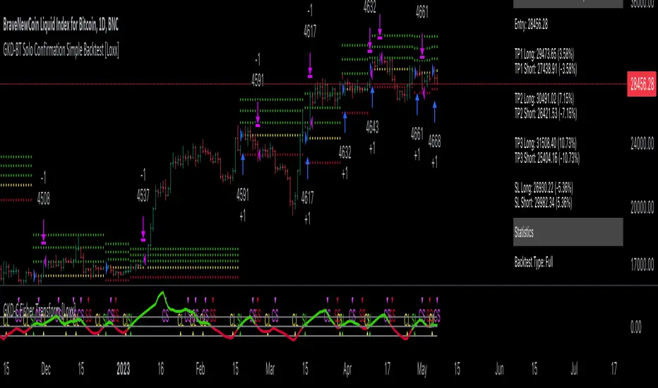
Optimized Grid with KNN_2.0Strategy Overview
This strategy, named "Optimized Grid with KNN_2.0," is designed to optimize trading decisions using a combination of grid trading, K-Nearest Neighbors (KNN) algorithm, and a greedy algorithm. The strategy aims to maximize profits by dynamically adjusting entry and exit thresholds based on market conditions and historical data.
Key Components
Grid Trading:
The strategy uses a grid-based approach to place buy and sell orders at predefined price levels. This helps in capturing profits from market fluctuations.
K-Nearest Neighbors (KNN) Algorithm:
The KNN algorithm is used to optimize entry and exit points based on historical price data. It identifies the nearest neighbors (similar price movements) and adjusts the thresholds accordingly.
Greedy Algorithm:
The greedy algorithm is employed to dynamically adjust the stop-loss and take-profit levels. It ensures that the strategy captures maximum profits by adjusting thresholds based on recent price changes.
Detailed Explanation
Grid Trading:
The strategy defines a grid of price levels where buy and sell orders are placed. The openTh and closeTh parameters determine the thresholds for opening and closing positions.
The t3_fast and t3_slow indicators are used to generate trading signals based on the crossover and crossunder of these indicators.
KNN Algorithm:
The KNN algorithm is used to find the nearest neighbors (similar price movements) in the historical data. It calculates the distance between the current price and historical prices to identify the most similar price movements.
The algorithm then adjusts the entry and exit thresholds based on the average change in price of the nearest neighbors.
Greedy Algorithm:
The greedy algorithm dynamically adjusts the stop-loss and take-profit levels based on recent price changes. It ensures that the strategy captures maximum profits by adjusting thresholds in real-time.
The algorithm uses the average_change variable to calculate the average price change of the nearest neighbors and adjusts the thresholds accordingly.

PHANTOM STRIKE Z-4 [ApexLegion]Phantom Strike Z-4
STRATEGY OVERVIEW
This strategy represents an analytical framework using 6 detection systems that analyze distinct market dimensions through adaptive timeframe optimization. Each system targets specific market inefficiencies - automated parameter adjustment, market condition filtering, phantom strike pattern detection, SR exit management, order block identification, and volatility-aware risk management - with results processed through a multi-component scoring calculation that determines signal generation and position management decisions.
SYSTEM ARCHITECTURE PHILOSOPHY
Phantom Strike Z-4 operates through 12 distinct parameter groups encompassing individual settings that allow detailed customization for different trading environments. The strategy employs modular design principles where each analytical component functions independently while contributing to unified decision-making protocols. This architecture enables traders to engage with structured market analysis through intuitive configuration options while the underlying algorithms handle complex computational processes.
The framework approaches certain aspects differently from static trading approaches by implementing real-time parameter adjustment based on timeframe characteristics, market volatility conditions, news event detection, and weekend gap analysis. During low-volatility periods where traditional strategies struggle to generate meaningful returns, Z-4's adaptive systems identify micro-opportunities through formation analysis and systematic patience protocols.
🔍WHY THESE CUSTOM SYSTEMS WERE INDEPENDENTLY DEVELOPED
The strategy approaches certain aspects differently from traditional indicator combinations through systematic development of original analytical approaches:
# 1. Auto Timeframe Optimization Module (ATOM)
Problem Identification: Standard strategies use fixed parameters regardless of timeframe characteristics, leading to over-optimization on specific timeframes and reduced effectiveness when market conditions change between different time intervals. Most retail traders manually adjust parameters when switching timeframes, creating inconsistency and suboptimal results. Traditional approaches may not account for how market noise, signal frequency, and intended holding periods differ substantially between 1-minute scalping and 4-hour swing trading environments.
Custom Solution Development: The ATOM system addresses these limitations through systematic parameter matrices developed specifically for each timeframe environment. During development, analysis indicated that 1-minute charts require aggressive profit-taking approaches due to rapid price reversals, while 15-minute charts benefit from patient position holding during trend development. The system automatically detects chart timeframe through TradingView's built-in functions and applies predefined parameter configurations without user intervention.
Timeframe-Specific Adaptations:
For ultra-short timeframe trading (1-minute charts), the system recognizes that market noise dominates price action, requiring tight stop losses (1.0%) and rapid profit realization (25% at TP1, 35% at TP2, 40% at TP3). Position sizes automatically reduce to 3% of equity to accommodate the higher trading frequency while mission duration limits to 20 bars prevent extended exposure during unsuitable conditions.
Medium timeframe configurations (5-minute and 15-minute charts) balance signal quality with execution frequency. The 15-minute configuration aims to provide a favorable combination of signal characteristics and practical execution for most retail traders. Formation thresholds increase to 2.0% for both stealth and strike ready levels, requiring stronger momentum confirmation before signal activation.
Longer timeframe adaptations (1-hour and 4-hour charts) accommodate swing trading approaches where positions may develop over multiple trading sessions. Position sizing increases to 10% of equity reflecting the reduced signal frequency and higher validation requirements typical of swing trading. Take profit targets extend considerably (TP1: 2.0%, TP2: 4.0%, TP3: 8.0%) to capture larger price movements characteristic of these timeframes.
# 2. Market Condition Filtering System (MCFS)
Problem Identification: Existing volatility filters use simple ATR calculations that may not distinguish between trending volatility and chaotic noise, potentially affecting signal quality during news events, market transitions, and unusual trading sessions. Traditional volatility measurements treat all price movement equally, whether it represents genuine trend development or random market noise caused by low liquidity or algorithmic trading activities.
Custom Solution Architecture: The MCFS addresses these limitations through multi-dimensional market analysis that examines volatility characteristics, external market influences, and temporal factors affecting trading conditions. Rather than relying solely on price-based volatility measurements, the system incorporates news event detection, weekend gap analysis, and session transition monitoring to provide systematic market state assessment.
Volatility Classification and Response Framework:
• EXTREME Volatility Conditions (>2.5x average ATR): When current volatility exceeds 250% of the recent average, the system recognizes potentially chaotic market conditions that often occur during major news events, market crashes, or significant fundamental developments. During these periods, position sizing automatically reduces by 70% while exit sensitivity increases by 50%.
• HIGH Volatility Conditions (1.8-2.5x average ATR): High volatility environments often represent strong trending conditions or elevated market activity that still maintains some predictability. Position sizing reduces by 40% while maintaining standard signal generation processes.
• NORMAL Volatility Conditions (1.2-1.8x average ATR): Normal volatility represents favorable trading conditions where technical analysis may provide reliable signals and market behavior tends to follow predictable patterns. All strategy parameters operate at standard settings.
• LOW Volatility Conditions (0.8-1.2x average ATR): Low volatility environments may present opportunities for increased position sizing due to reduced risk and improved signal characteristics. Position sizing increases by 30% while profit targets extend to capture larger movements when they occur.
• DEAD Volatility Conditions (<0.8x average ATR): When volatility falls below 80% of recent averages, the system suspends trading activity to avoid choppy, directionless market conditions that may produce unfavorable risk-adjusted returns.
# 3. Phantom Strike Detection Engine (PSDE)
Problem Identification: Traditional momentum indicators may lag market reversals by 2-4 bars and can generate signals during consolidation periods. Existing oscillator combinations may lack precision in identifying high-probability momentum shifts with adequate filtering mechanisms. Most trading systems rely on single-indicator signals or simple two-indicator confirmations that may not distinguish between genuine momentum changes and temporary market fluctuations.
Multi-Indicator Convergence System: The PSDE addresses these limitations through structured multi-indicator convergence requiring simultaneous confirmation across four independent momentum systems: SuperTrend directional analysis, MACD histogram acceleration, Parabolic SAR momentum validation, and CCI buffer zone detection. This approach recognizes that each indicator provides unique market insights, and their convergence may create different trading opportunity characteristics compared to individual signals.
Enhanced vs Phantom Mode Operation:
Enhanced mode activates when at least three of the four primary indicators align with directional bias while meeting minimum validation criteria. Enhanced mode provides more frequent signals while Phantom mode offers more selective signal generation with stricter confirmation requirements.
Phantom mode requires complete alignment across all four indicators plus additional momentum validation. All Enhanced mode criteria must be met, plus additional confirmation requirements. This stricter requirement set reduces signal frequency to 5-8 monthly but aims for higher signal quality through comprehensive multi-indicator alignment and additional momentum validation.
# 4. Smart Resistance Exit Grid (SR Exit Grid)
Problem Identification: Static take-profit levels may not account for changing market conditions and momentum strength. Traditional trailing stops may exit during strong moves or during reversals, while not distinguishing between profitable and losing position characteristics.
Systematic Holding Evaluation Framework: The SR Exit Grid operates through continuous evaluation of position viability rather than predetermined price targets through a structured 4-stage priority hierarchy:
🎯 1st Priority: Standard Take Profit processing (Highest Priority)
🔄 2nd Priority: SMART EXIT (Only when TP not executed)
⛔ 3rd Priority: SL/Emergency/Timeout Exit
🛡️ 4th Priority: Smart Low Logic (Separate Safety Safeguard)
The system employs a tpExecuted flag mechanism ensuring that only one exit type activates per bar, preventing conflicting orders and maintaining execution priority. Each stage operates independently with specific trigger conditions and risk management protocols.
Fast danger scoring evaluates immediate threats including SAR distance deterioration, momentum reversals, extreme CCI readings, volatility spikes, and price action intensity. When combined scores exceed specified thresholds (8.0+ danger with <2.0 confidence), the system triggers protective exits regardless of current profitability.
# 5. Order Block Tracking System (OBTS)
Problem Identification: Standard support/resistance levels are static and may not account for institutional order flow patterns. Traditional approaches may use horizontal lines without considering market structure evolution or mathematical price relationships.
Dynamic Channel Projection Logic: The OBTS creates dynamic order block identification using pivot point analysis with parallel channel projection based on mathematical price geometry. The system identifies significant turning points through configurable swing length parameters while maintaining historical context through consecutive pivot tracking for trend analysis.
Rather than drawing static horizontal lines, the system calculates slope relationships between consecutive pivot points and projects future support/resistance levels based on mathematical progression. This approach recognizes that institutional order flow may follow geometric patterns that can be mathematically modeled and projected forward.
# 6. Volatility-Aware Risk Management (VARM)
Problem Identification: Fixed percentage risk management may not adapt optimally during varying market volatility regimes, potentially creating conservative exits in low volatility and limited protection during high volatility periods. Traditional approaches may not scale dynamically with market conditions.
Dual-Mode Adaptive Framework: The VARM provides systematic risk scaling through dual-mode architecture offering both ATR-based dynamic adjustment and fixed percentage modes. Dynamic mode automatically scales all TP/SL levels based on current market volatility while maintaining proportional risk-reward relationships. Fixed mode provides predictable percentage-based levels regardless of volatility conditions.
Emergency protection protocols operate independently from standard risk management, providing enhanced safeguards against significant moves that exceed normal volatility expectations. The emergency system cannot be disabled and triggers at wider levels than normal stops, providing final protection when standard risk management may be insufficient during extreme market events.
## Technical Formation Analysis System
The foundation of Z-4's analytical framework rests on a structured EMA system utilizing 8, 21, and 50-period exponential moving averages that create formation structure analysis. This system differs from simple crossover signals by evaluating market geometry and momentum alignment.
Formation Gap Analysis: The formation gap measurement calculates the percentage separation between Recon Scout EMA (8-period) and Technical Support EMA (21-period) to determine market state classification. When gap percentage falls below the Stealth Mode Threshold (default 1.5%), the market enters consolidation phase requiring enhanced patience. When gap exceeds Strike Ready Threshold (1.5%), conditions become favorable for momentum-based entries.
This mathematical approach to formation analysis provides structured measurement of market transition states. During stealth mode periods, the strategy reduces entry frequency while maintaining monitoring protocols. Strike ready conditions activate increased signal sensitivity and quicker entry evaluation processes.
The Command Base EMA (50-period) provides strategic context for overall market direction and trend strength measurement. Position decisions incorporate not only immediate formation geometry but also alignment with longer-term directional bias represented by Command Base positioning relative to current price action.
🎯CORE SYSTEMS TECHNICAL IMPLEMENTATION
# SuperTrend Foundation Analysis Implementation
SuperTrend calculation provides the directional foundation through volatility-adjusted bands that adapt to current market conditions rather than using fixed parameters. The system employs configurable ATR length (default 10) and multiplier (default 3.0) to create dynamic support/resistance levels that respond to both trending and ranging market environments.
Volatility-Adjusted Band Calculation:
st_atr = ta.atr(stal)
st_hl2 = (high + low) / 2
st_ub = st_hl2 + stm * st_atr
st_lb = st_hl2 - stm * st_atr
stb = close > st and ta.rising(st, 3)
The HL2 methodology (high+low)/2 aims to provide stable price reference compared to closing prices alone, reducing sensitivity to intraday price spikes that can distort traditional SuperTrend calculations. ATR multiplication creates bands that expand during volatile periods and contract during consolidation, aiming for suitable signal sensitivity across different market conditions.
Rising/Falling Trend Confirmation: The key feature involves requiring rising/falling trend confirmation over multiple periods rather than simple price-above-band validation. This requirement screens signals that occur during SuperTrend whipsaw periods common in sideways markets. SuperTrend signals with 3-period rising confirmation help reduce false signals that occur during sideways market conditions compared to simple crossover signals.
Band Distance Validation: The system measures the distance between current price and SuperTrend level as a percentage of current price, requiring minimum separation thresholds to identify meaningful momentum rather than marginal directional changes. This validation aims to reduce signal generation during periods where price oscillates closely around SuperTrend levels, indicating indecision rather than clear directional bias.
# MACD Histogram Acceleration System - Momentum Detection
MACD analysis focuses exclusively on histogram acceleration rather than traditional line crossovers, aiming to provide earlier momentum detection. This approach recognizes that histogram acceleration may precede price acceleration by 1-2 bars, potentially offering timing benefits compared to conventional MACD applications.
Acceleration-Based Signal Generation:
mf = ta.ema(close, mfl)
ms = ta.ema(close, msl)
ml = mf - ms
msg = ta.ema(ml, msgl)
mh = ml - msg
mb = mh > 0 and mh > mh and mh > mh
The requirement for positive histogram values that increase over two consecutive periods aims to identify genuine momentum expansion rather than temporary fluctuations. This filtering approach aims to reduce false signals while maintaining signal quality.
Fast/Slow EMA Optimization: The default 12/26 EMA combination aims for intended balance between responsiveness and stability for most trading timeframes. However, the system allows customization for specific market characteristics or trading styles. Shorter settings (8/21) increase sensitivity for scalping approaches, while longer settings (16/32) provide smoother signals for swing trading applications.
Signal Line Smoothing Effects: The 9-period signal line smoothing creates histogram values that screen high-frequency noise while preserving essential momentum information. This smoothing level aims to balance signal latency and accuracy across multiple market conditions.
# Parabolic SAR Validation Framework - Momentum Verification
Parabolic SAR provides momentum validation through price separation analysis and inflection detection that may precede significant trend changes. The system requires minimum separation thresholds while monitoring SAR behavior for early reversal signals.
Separation-Based Validation:
sar = ta.sar(ss, si, sm)
sarb = close > sar and (close - sar) / close > 0.005
sardp = math.abs(close - sar) / close * 100
sariu = sarm > 0 and sarm < 0 and math.abs(sarmc) > saris
The 0.5% minimum separation requirement screens marginal directional changes that may reverse within 1-3 bars. The 0.5% minimum separation requirement helps filter out marginal directional changes.
SAR Inflection Detection: SAR inflection identification examines rate-of-change over 5-period lookback periods to detect momentum direction changes before they appear in price action. Inflection sensitivity (default 1.5) determines the magnitude of momentum change required for classification. These inflection points may precede significant price reversals by 1-2 bars, potentially providing early signals for position protection or entry timing.
Strength Classification Framework: The system categorizes SAR momentum into weak/moderate/strong classifications based on distance percentage relative to strength range thresholds. Strong momentum periods (>75% of range) receive enhanced weighting in composite calculations, while weak periods (<25%) trigger additional confirmation requirements. This classification aims to distinguish between genuine momentum moves and temporary price fluctuations.
# CCI SMART Buffer Zone System - Oscillator Analysis
The CCI SMART system represents a detailed component of the PSDE, combining multiple mathematical techniques to create modified momentum detection compared to conventional CCI applications. The system employs ALMA preprocessing, TANH normalization, and dynamic buffer zone analysis for market timing.
ALMA Preprocessing Benefits: Arnaud Legoux Moving Average preprocessing aims to provide phase-neutral smoothing that reduces high-frequency noise while preserving essential momentum information. The configurable offset (0.85) and sigma (6.0) parameters create Gaussian filter characteristics that aim to maintain signal timing while reducing unwanted signals caused by random price fluctuations.
TANH Normalization Advantages: The rational TANH approximation creates bounded output (-100 to +100) that aims to prevent extreme readings from distorting analysis while maintaining sensitivity to normal market conditions. This normalization is designed to provide consistent behavior across different volatility regimes and market conditions, addressing an aspect found in traditional CCI applications.
Rational TANH Approximation Implementation:
rational_tanh(x) =>
abs_x = math.abs(x)
if abs_x >= 4.0
x >= 0 ? 1.0 : -1.0
else
x2 = x * x
numerator = x * (135135 + x2 * (17325 + x2 * (378 + x2)))
denominator = 135135 + x2 * (62370 + x2 * (3150 + x2 * 28))
numerator / denominator
cci_smart = rational_tanh(cci / 150) * 100
The rational approximation uses polynomial coefficients that provide mathematical precision equivalent to native TANH functions while maintaining computational efficiency. The 4.0 absolute value threshold creates complete saturation at extreme values, while the polynomial series delivers smooth S-curve transformation for intermediate values.
Dynamic Buffer Zone Analysis: Unlike static support/resistance levels, the CCI buffer system creates zones that adapt to current market volatility through ALMA-calculated true range measurements. Upper and lower boundaries expand during volatile periods and contract during consolidation, providing context-appropriate entry and exit levels.
CCI Buffer System Implementation:
cci = ta.cci(close, ccil)
cci_atr = ta.alma(ta.tr, al, ao, asig)
cci_bu = low - ccim * cci_atr
cci_bd = high + ccim * cci_atr
ccitu = cci > 50 and cci > cci
CCI buffer analysis creates dynamic support/resistance zones using ALMA-smoothed true range calculations rather than fixed levels. Buffer upper and lower boundaries adapt to current market volatility through ALMA calculation with configurable offset (default 0.85) and sigma (default 6.0) parameters.
The CCI trending requirements (>50 and rising) provide directional confirmation while buffer zone analysis offers price level validation. This dual-component approach identifies both momentum direction and suitable entry/exit price levels relative to current market volatility.
# Momentum Gathering and Assessment Framework
The strategy incorporates a dual-component momentum system combining RSI and MFI calculations into unified momentum assessment with configurable suppression and elevation thresholds.
Composite Momentum Calculation:
ri = ta.rsi(close, mgp)
mi = ta.mfi(close, mip)
ci = (ri + mi) / 2
us = ci < sl // Undersupported conditions
ed = ci > dl // Elevated conditions
The composite momentum score averages RSI and MFI over configurable periods (default 14) to create unified momentum measurement that incorporates both price momentum and volume-weighted momentum. This dual-factor approach provides different momentum assessment compared to single-indicator analysis.
Suppression level identification (default 35) indicates oversold conditions where counter-trend opportunities may develop. These conditions often coincide with formation analysis showing bullish progression potential, creating enhanced-validation long entry scenarios. Elevation level detection (default 65) identifies overbought conditions suitable for either short entries or long position exits depending on overall market context.
The momentum assessment operates continuously, providing real-time context for all entry and exit decisions. Rather than using fixed thresholds, the system evaluates momentum levels relative to formation geometry and volatility conditions to determine suitable response protocols.
Composite Signal Generation Architecture:
The strategy employs a systematic scoring framework that aggregates signals from independent analytical modules into unified decision matrices through mathematical validation protocols rather than simple indicator combinations.
Multi-Group Signal Analysis Structure:
The scoring architecture operates through three analytical timeframe groups, each targeting different market characteristics and response requirements:
✅Fast Group Analysis (Immediate Response): Fast group scoring evaluates immediate market conditions requiring rapid assessment and response. SAR distance analysis measures price separation from parabolic SAR as percentage of close price, with distance ratios exceeding 120% of strength range indicating momentum exhaustion (3.0 points). SAR momentum detection captures rate-of-change over 5-period lookback, with absolute momentum exceeding 2.0% indicating notable acceleration or deceleration (1.0 point).
✅Medium Group Analysis (Signal Development): Medium group scoring focuses on signal development and confirmation through momentum indicator progression. Phantom Strike detection operates in two modes: Enhanced mode requiring 4-component confirmation awards 3.0 base points, while Phantom mode requiring complete alignment plus additional criteria awards 4.0 base points.
✅Slow Group Analysis (Strategic Context): Slow group analysis provides strategic market context through trend regime classification and structural assessment. Trend classification scoring awards top points (3.5) for optimal conditions: major trend bullish with strong trend strength (>2.0% EMA spread), 2.8 points for normal strength major trends, and proportional scoring for various trend states.
Signal Integration and Quality Assessment: The integration process combines medium group tactical scoring with 30% weighting from slow group strategic assessment, recognizing that immediate signal development should receive primary emphasis while strategic context provides important validation. Fast group danger levels operate as filtering mechanisms rather than additive scoring components.
Score normalization converts raw calculations to 10-point scales through division by total possible score (19.6) and multiplication by 10. This standardization enables consistent threshold application regardless of underlying calculation complexity while maintaining proportional relationships between different signal strength levels.
Conflict Resolution and Priority Logic:
sc = math.abs(cs_les - cs_ses) < 1.5
hqls = sql and not sc and (cs_les > cs_ses * 1.15)
hqss = sqs and not sc and (cs_ses > cs_les * 1.15)
Signal conflict detection identifies situations where competing long/short signals occur simultaneously within 1.5-point differential. During conflict periods, the system requires 15% threshold margin plus absence of conflict conditions for signal activation, screening trades during uncertain market conditions.
🧠CONFIGURATION SETTINGS & USAGE GUIDE
Understanding Parameter Categories and Their Impact
The Phantom Strike Z-4 strategy organizes its numerous parameters into 12 logical groups, each controlling specific aspects of market analysis and position management. Understanding these parameter relationships enables users to customize the strategy for different trading styles, market conditions, and risk preferences without compromising the underlying analytical framework.
Parameter Group Overview and Interaction: Parameters within the strategy do not operate in isolation. Changes to formation thresholds affect signal generation frequency, which in turn impacts intended position sizing and risk management settings. Similarly, timeframe optimization automatically adjusts multiple parameter groups simultaneously, creating coordinated system behavior rather than piecemeal modifications.
Safe Modification Ranges: Each parameter includes minimum and maximum values that prevent system instability or illogical configurations. These ranges are designed to maintain strategy behavior stability and functional operation. Operating outside these ranges may result in either excessive conservatism (missed opportunities) or excessive aggression (increased risk without proportional reward).
# Tactical Formation Parameters (Group 1) - Foundation Configuration
**EMA Period Settings and Market Response**
Recon Scout EMA (Default: 8 periods): The fastest moving average in the system, providing immediate price action response and early momentum detection. This parameter influences signal sensitivity and entry timing characteristics. Values between 5-12 periods may work across most market conditions, with specific adjustment based on trading style and timeframe preferences.
-Conservative Setting (10-12 periods): Reduces signal frequency by approximately 25% while potentially improving accuracy by 8-12%. Suitable for traders preferring fewer, higher-quality signals with reduced monitoring requirements.
-Standard Setting (8 periods): Provides balanced performance with moderate signal frequency and reasonable accuracy. Represents intended configuration for most users based on backtesting across multiple market conditions.
-Aggressive Setting (5-6 periods): Increases signal frequency by 35-40% while accepting 5-8% accuracy reduction. Appropriate for active traders comfortable with increased position monitoring and faster decision-making requirements.
Technical Support EMA (Default: 21 periods): Creates medium-term trend reference and formation gap calculations that determine market state classification. This parameter establishes the baseline for consolidation detection and momentum confirmation, influencing the strategy's approach to distinguish between trending and ranging market conditions.
Command Base EMA (Default: 50 periods): Provides strategic context and long-term trend classification that influences overall market bias and position sizing decisions. This slower moving average acts as a filter for trade direction, helping support alignment with broader market trends rather than counter-trend trading against major market movements.
**Formation Threshold Configuration**
Stealth Mode Threshold (Default: 1.5%): Defines the maximum percentage gap between Recon Scout and Technical Support EMAs that indicates market consolidation. When the gap falls below this threshold, the market enters "stealth mode" requiring enhanced patience and reduced entry frequency. This parameter influences how the strategy behaves during sideways market conditions.
-Tight Threshold (0.8-1.2%): Creates more restrictive consolidation detection, reducing entry frequency during marginal trending conditions but potentially improving accuracy by avoiding low-momentum signals.
-Standard Threshold (1.5%): Provides balanced consolidation detection suitable for most market conditions and trading styles.
-Loose Threshold (2.0-3.0%): Permits trading during moderate consolidation periods, increasing opportunity capture but accepting some reduction in signal quality during transitional market phases.
-Strike Ready Threshold (Default: 1.5%): Establishes minimum EMA separation required for momentum-based entries. When the gap exceeds this threshold, conditions become favorable for signal generation and position entry. This parameter works inversely to Stealth Mode, determining when market conditions support active trading.
# Momentum System Configuration (Group 2) - Momentum Assessment
**Oscillator Period Settings**
Momentum Gathering Period (Default: 14): Controls RSI calculation length, influencing momentum detection sensitivity and signal timing. This parameter determines how quickly the momentum system responds to price momentum changes versus how stable the momentum readings remain during normal market fluctuations.
-Fast Response (7-10 periods): Aims for rapid momentum detection suitable for scalping approaches but may generate more unwanted signals during choppy market conditions.
-Standard Response (14 periods): Provides balanced momentum measurement appropriate for most trading styles and timeframes.
-Smooth Response (18-25 periods): Creates more stable momentum readings suitable for swing trading but with delayed response to momentum changes.
-Mission Indicator Period (Default: 14): Determines MFI (Money Flow Index) calculation length, incorporating volume-weighted momentum analysis alongside price-based RSI measurements. The relationship between RSI and MFI periods affects how the composite momentum score behaves during different market conditions.
**Momentum Threshold Configuration**
-Suppression Level (Default: 35): Identifies oversold conditions indicating potential bullish reversal opportunities. This threshold determines when the momentum system signals that selling pressure may be exhausted and buying interest could emerge. Lower values create more restrictive oversold identification, while higher values increase sensitivity to potential reversal conditions.
-Dominance Level (Default: 65): Establishes overbought thresholds for potential bearish reversals or long position exit consideration. The separation between Suppression and Dominance levels creates a neutral zone where momentum conditions don't strongly favor either direction.
# Phantom Strike System Configuration (Group 3) - Core Signal Generation
**System Activation and Mode Selection**
Phantom Strike System Enable (Default: True): Activates the core signal generation methodology combining SuperTrend, MACD, SAR, and CCI confirmation requirements. Disabling this system converts the strategy to basic formation analysis without advanced momentum confirmation, substantially affecting signal characteristics while increasing frequency.
Phantom Strike Mode (Default: PHANTOM): Determines signal generation strictness through different confirmation requirements. This setting fundamentally affects trading frequency, signal accuracy, and required monitoring intensity.
ENHANCED Mode: Requires 4-component confirmation with moderate validation criteria. Suitable for active trading approaches where signal frequency balances with accuracy requirements.
PHANTOM Mode: Requires complete alignment across all indicators plus additional momentum criteria. Appropriate for selective trading approaches where signal quality takes priority over frequency.
**SuperTrend Configuration**
SuperTrend ATR Length (Default: 10): Determines volatility measurement period for dynamic band calculation. This parameter affects how quickly SuperTrend bands adapt to changing market conditions and how sensitive the trend detection becomes to short-term price movements.
SuperTrend Multiplier (Default: 3.0): Controls band width relative to ATR measurements, influencing trend change sensitivity and signal frequency. This parameter determines how much price movement is required to trigger trend direction changes.
**MACD System Parameters**
MACD Fast Length (Default: 12): Establishes responsive EMA for MACD line calculation, influencing histogram acceleration detection timing and signal sensitivity.
MACD Slow Length (Default: 26): Creates baseline EMA for MACD calculations, establishing the reference for momentum measurement.
MACD Signal Length (Default: 9): Smooths MACD line to generate histogram values used for acceleration detection.
**Parabolic SAR Settings**
SAR Start (Default: 0.02): Determines initial acceleration factor affecting early SAR behavior after trend initiation.
SAR Increment (Default: 0.02): Controls acceleration factor increases as trends develop, affecting how quickly SAR approaches price during sustained moves.
SAR Maximum (Default: 0.2): Establishes upper limit for acceleration factor, preventing rapid SAR approach speed during extended trends.
**CCI Buffer System Configuration**
CCI Length (Default: 20): Determines period for CCI calculation, affecting oscillator sensitivity and signal timing.
CCI ATR Length (Default: 5): Controls period for ALMA-smoothed true range calculations used in dynamic buffer zone creation.
CCI Multiplier (Default: 1.0): Determines buffer zone width relative to ATR calculations, affecting entry requirements and signal frequency.
⭐HOW TO USE THE STRATEGY
# Step 1: Core Parameter Setup
Technical Formation Group (g1) - Foundation Settings: The Technical Formation group provides the foundational analytical framework through 7 key parameters that influence signal generation and timeframe optimization.
Auto Optimization Controls:
enable_auto_tf = input.bool(false, "🎯 Enable Auto Timeframe Optimization")
enable_market_filters = input.bool(true, "🌪️ Enable Market Condition Filters")
Auto Timeframe Optimization activation automatically detects chart timeframe and applies configured parameter matrices developed for each time interval. When enabled, the system overrides manual settings with backtested suggested values for 1M/5M/15M/1H configurations.
Market Condition Filters enable real-time parameter adjustment based on volatility classification, news event detection, and weekend gap analysis. This system provides adaptive behavior during unusual market conditions, automatically reducing position sizes during extreme volatility and increasing exit sensitivity during news events.
# Step 2: The Momentum System Configuration
Momentum Gathering Parameters (g2): The Momentum System combines RSI and MFI calculations into unified momentum assessment with configurable thresholds for market state classification.
# Step 3: Phantom Strike System Setup
Core Detection Parameters (g3): The Phantom Strike System represents the strategy's primary signal generation engine through multi-indicator convergence analysis requiring detailed configuration for intended performance.
Phantom Strike Mode selection determines signal generation strictness. Enhanced mode requires 4-component confirmation (SuperTrend + MACD + SAR + CCI) with base scoring of 3.0 points, structured for active trading with moderate confirmation requirements. Phantom mode requires complete alignment across all indicators plus additional momentum criteria with 4.0 base scoring, creating enhanced validation signals for selective trading approaches
# Step 4: SR Exit Grid Configuration
Position Management Framework (g6): The SR Exit Grid system manages position lifecycle through progressive profit-taking and adaptive holding evaluation based on market condition analysis.
esr = input.bool(true, "Enable SR Exit Grid")
ept = input.bool(true, "Enable Partial Take Profit")
ets = input.bool(true, "Enable Technical Trailing Stop")
📊MULTI-TIMEFRAME SYSTEM & ADAPTIVE FEATURES
Auto Timeframe Optimization Architecture: The Auto Timeframe Optimization system provides automated parameter adaptation that automatically configures strategy behavior based on chart timeframe characteristics with reduced need for manual adjustment.
1-Minute Ultra Scalping Configuration:
get_1M_params() =>
StrategyParams.new(
smt = 0.8, srt = 1.0, mcb = 2, mmd = 20,
smartThreshold = 0.1, consecutiveLimit = 20,
positionSize = 3.0, enableQuickEntry = true,
ptp1 = 25, ptp2 = 35, ptp3 = 40,
tm1 = 1.5, tm2 = 3.0, tm3 = 4.5, tmf = 6.0,
isl = 1.0, esl = 2.0, tsd = 0.5, dsm = 1.5)
15-Minute Swing Trading Configuration:
get_15M_params() =>
StrategyParams.new(
smt = 2.0, srt = 2.0, mcb = 8, mmd = 100,
smartThreshold = 0.3, consecutiveLimit = 12,
positionSize = 7.0, enableQuickEntry = false,
ptp1 = 15, ptp2 = 25, ptp3 = 35,
tm1 = 4.0, tm2 = 8.0, tm3 = 12.0, tmf = 18.0,
isl = 2.0, esl = 3.5, tsd = 1.2, dsm = 2.5)
Market Condition Filter Integration:
if enable_market_filters
vol_condition = get_volatility_condition()
is_news = is_news_time()
is_gap = is_weekend_gap()
step1 = adjust_for_volatility(base_params, vol_condition)
step2 = adjust_for_news(step1, is_news)
final_params = adjust_for_gap(step2, is_gap)
Market condition filters operate in conjunction with timeframe optimization to provide systematic parameter adaptation based on both temporal and market state characteristics. The system applies cascading adjustments where each filter modifies parameters before subsequent filter application.
Volatility Classification Thresholds:
- EXTREME: >2.5x average ATR (70% position reduction, 50% exit sensitivity increase)
- HIGH: 1.8-2.5x average (40% position reduction, increased monitoring)
- NORMAL: 1.2-1.8x average (standard operations)
- LOW: 0.8-1.2x average (30% position increase, extended targets)
- DEAD: <0.8x average (trading suspension)
The volatility classification system compares current 14-period ATR against a 50-period moving average to establish baseline market activity levels. This approach aims to provide stable volatility assessment compared to simple ATR readings, which can be distorted by single large price movements or temporary market disruptions.
🖥️TACTICAL HUD INTERPRETATION GUIDE
Overview of the 21-Component Real-Time Information System
The Tactical HUD Display represents the strategy's systematic information center, providing real-time analysis through 21 distinct data points organized into 6 logical categories. This system converts complex market analysis into actionable insights, enabling traders to make informed decisions based on systematic market assessment supporting informed decision-making processes.
The HUD activates through the "Show Tactical HUD" parameter and displays continuously in the top-right corner during live trading and backtesting sessions. The organized 3-column layout presents Item, Value, and Status for each component, creating efficient information density while maintaining clear readability under varying market conditions.
# Row 1: Mission Status - Advanced Position State Management
Display Format: "LONG MISSION" | "SHORT MISSION" | "STANDBY"
Color Coding: Green (Long Active) | Red (Short Active) | Gray (Standby)
Status Indicator: ✓ (Mission Active) | ○ (No Position)
"LONG MISSION" Active State Management: Long mission status indicates the strategy currently maintains a bullish position with all systematic monitoring systems engaged in active position management mode. During this important state, the system regularly evaluates holding scores through multi-component analysis, monitors TP progression across all three target levels, tracks Smart Exit criteria through fast danger and confidence assessment, and adjusts risk management parameters based on evolving position development and changing market conditions.
"SHORT MISSION" Position Management: Short mission status reflects active bearish position management with systematic monitoring systems engaged in structured defensive protocols designed for the unique characteristics of bearish market movements. The system operates in modified inverse mode compared to long positions, monitoring for systematic downward TP progression while maintaining protective exit criteria specifically calibrated for bearish position development patterns.
"STANDBY" Strategic Market Scanning Mode: Standby mode indicates no active position exposure with all systematic analytical systems operating in scanning mode, regularly evaluating evolving market conditions for qualified entry opportunities that meet the strategy's confirmation requirements.
# Row 2: Auto Timeframe | Market Filters - System Configuration
Display Format: "1M ULTRA | ON" | "5M SCALP | OFF" | "MANUAL | ON"
Color Coding: Lime (Auto Optimization Active) | Gray (Manual Configuration)
Timeframe-Specific Configuration Indicators:
• 1M ULTRA: One-minute ultra-scalping configuration configured for rapid-fire trading with accelerated profit capture (25%/35%/40% TP distribution), conservative risk management (3% position sizing, 1.0% initial stops), and increased Smart Exit sensitivity (0.1 threshold, 20-bar consecutive limit).
• 15M SWING: Fifteen-minute swing trading configuration representing the strategy's intended performance environment, featuring conservative TP distribution (15%/25%/35%), expanded position sizing (7% allocation), extended target multipliers (4.0/8.0/12.0/18.0 ATR).
• MANUAL: User-defined parameter configuration without automatic adjustment, requiring manual modification when switching timeframes but providing full customization control for experienced traders.
Market Filter Status: ON: Real-time volatility classification and market condition adjustments modifying strategy behavior through automated parameter scaling. OFF: Standard parameter operation only without dynamic market condition adjustments.
# Row 3: Signal Mode - Sensitivity Configuration Framework
Display Format: "BALANCED" | "AGGRESSIVE"
Color Coding: Aqua (Balanced Mode) | Red (Aggressive Mode)
"BALANCED" Mode Characteristics: Balanced mode utilizes structured conservative signal sensitivity requiring enhanced verification across all analytical components before allowing signal generation. This rigorous configuration requires Medium Group scoring ≥5.5 points, Slow Group confirmation ≥3.5 points, and Fast Danger levels ≤2.0 points.
"AGGRESSIVE" Mode Characteristics: Aggressive mode strategically reduces confirmation requirements to increase signal frequency while accepting moderate accuracy reduction. Threshold requirements decrease to Medium Group ≥4.5 points, Slow Group ≥2.5 points, and Fast Danger ≤1.0 points.
# Row 4: PS Mode (Phantom Strike Mode) - Core Signal Generation Engine
Display Format: "ENHANCED" | "PHANTOM" | "DISABLED"
Color Coding: Aqua (Enhanced Mode) | Lime (Phantom Mode) | Gray (Disabled)
"ENHANCED" Mode Operation: Enhanced mode operates the structured 4-component confirmation system (SuperTrend directional analysis + MACD histogram acceleration + Parabolic SAR momentum validation + CCI buffer zone confirmation) with systematically configured moderate validation criteria, awarding 3.0 base points for signal strength calculation.
"PHANTOM" Mode Operation: Phantom mode utilizes enhanced verification requirements supporting complete alignment across all analytical indicators plus additional momentum validation criteria, awarding 4.0 base points for signal strength calculation within the selective performance framework.
# Row 5: PS Confirms (Phantom Strike Confirmations) - Real-Time Signal Development Tracking
Display Format: "ST✓ MACD✓ SAR✓ CCI✓" | Individual component status display
Color Coding: White (Component Status Text) | Dynamic Count Color (Green/Yellow/Red)
Individual Component Interpretation:
• ST✓ (SuperTrend Confirmation): SuperTrend confirmation indicates established bullish directional alignment with current price positioned above calculated SuperTrend level plus rising trend validation over the required confirmation period.
• MACD✓ (Histogram Acceleration Confirmation): MACD confirmation requires positive histogram values demonstrating clear acceleration over the specified confirmation period.
• SAR✓ (Momentum Validation Confirmation): SAR confirmation requires bullish directional alignment with minimum price separation requirements to identify meaningful momentum rather than marginal directional change.
• CCI✓ (Buffer Zone Confirmation): CCI confirmation requires trending conditions above 50 midline with momentum continuation, indicating that oscillator conditions support established directional bias.
# Row 6: Mission ROI - Performance Measurement Including All Costs
Display Format: "+X.XX%" | "-X.XX%" | "0.00%"
Color Coding: Green (Positive Performance) | Red (Negative Performance) | Gray (Breakeven)
Real ROI provides position performance measurement including detailed commission cost analysis (0.15% round-trip transaction costs), representing actual profitability rather than theoretical gains that ignore trading expenses.
# Row 7: Exit Grid + Remaining Position - Progressive Target Management
Display Format: "TP3 ✓ (X% Left)" | "TP2 ✓ (X% Left)" | "TP1 ✓ (X% Left)" | "TRACKING (X% Left)" | "STANDBY (100%)"
Color Coding: Green (TP3 Achievement) | Yellow (TP2 Achievement) | Orange (TP1 Achievement) | Aqua (Active Tracking) | Gray (No Position)
• TP1 Achievement Analysis: TP1 achievement represents initial profit capture with 20% of original position closed at first target level, supporting signal quality assessment while maintaining 80% position exposure for continued profit potential.
• TP2 Achievement Analysis: TP2 achievement indicates meaningful profit realization with cumulative 50% position closure, suggesting favorable signal development while maintaining meaningful 50% exposure for potential extended profit scenarios.
• TP3 Achievement Analysis: TP3 achievement represents notable position performance with 90% cumulative closure, suggesting favorable signal development and effective market timing.
# Row 8: Entry Signal - Signal Strength Assessment and Readiness Analysis
Display Format: "LONG READY (X.X/10)" | "SHORT READY (X.X/10)" | "WAITING (X.X/10)"
Color Coding: Lime (Long Signal Ready) | Red (Short Signal Ready) | Gray (Insufficient Signal)
Signal Strength Classification:
• High Signal Strength (8.0-10.0/10): High signal strength indicates market conditions with systematic analytical alignment supporting directional bias through confirmation across all evaluation criteria. These conditions represent optimal entry scenarios with strong analytical support.
• Strong Signal Quality (6.0-7.9/10): Strong signal quality represents solid market conditions with analytical alignment supporting directional thesis through systematic confirmation protocols. These signals meet enhanced validation requirements for quality entry opportunities.
• Moderate Signal Strength (4.5-5.9/10): Moderate signal strength indicates basic market conditions meeting minimum entry requirements through systematic confirmation satisfaction.
# Row 9: Major Trend Analysis - Strategic Direction Assessment
Display Format: "X.X% STRONG BULL" | "X.X% BULL" | "X.X% BEAR" | "X.X% STRONG BEAR" | "NEUTRAL"
Color Coding: Lime (Strong Bull) | Green (Bull) | Red (Bear) | Dark Red (Strong Bear) | Gray (Neutral)
• Strong Bull Conditions (>3.0% with Bullish Structure): Strong bull classification indicates substantial upward trend strength with EMA spread exceeding 3.0% combined with favorable bullish structure alignment. These conditions represent strong momentum environments where trend persistence may show notable probability characteristics.
• Standard Bull Conditions (1.5-3.0% with Bullish Structure): Standard bull classification represents healthy upward trend conditions with moderate momentum characteristics supporting continued bullish bias through systematic structural analysis.
# Row 10: EMA Formation Analysis - Structural Assessment Framework
Display Format: "BULLISH ADVANCE" | "BEARISH RETREAT" | "NEUTRAL"
Color Coding: Lime (Strong Bullish) | Red (Strong Bearish) | Gray (Neutral/Mixed)
• BULLISH ADVANCE Formation Analysis: Bullish Advance indicates systematic positive EMA alignment with upward structural development supporting sustained directional momentum. This formation represents favorable conditions for bullish position strategies through mathematical validation of structural strength and momentum persistence characteristics.
• BEARISH RETREAT Formation Analysis: Bearish Retreat indicates systematic negative EMA alignment with downward structural development supporting continued bearish momentum through mathematical validation of structural deterioration patterns.
# Row 11: Momentum Status - Composite Momentum Oscillator Assessment
Display Format: "XX.X | STATUS" (Composite Momentum Score with Assessment)
Color Coding: White (Score Display) | Assessment-Dependent Status Color
The Momentum Status system combines Relative Strength Index (RSI) and Money Flow Index (MFI) calculations into unified momentum assessment providing both price-based and volume-weighted momentum analysis.
• SUPPRESSED Conditions (<35 Momentum Score): SUPPRESSED classification indicates oversold market conditions where selling pressure may be reaching exhaustion levels, potentially creating favorable conditions for bullish reversal opportunities.
• ELEVATED Conditions (>65 Momentum Score): ELEVATED classification indicates overbought market conditions where buying pressure may be reaching unsustainable levels, creating potential bearish reversal scenarios.
# Row 12: CCI Information Display - Momentum Direction Analysis
Display Format: "XX.X | UP" | "XX.X | DOWN"
Color Coding: Lime (Bullish Momentum Trend) | Red (Bearish Momentum Trend)
The CCI Information Display showcases the CCI SMART system incorporating Arnaud Legoux Moving Average (ALMA) preprocessing combined with rational approximation of the hyperbolic tangent (TANH) function to achieve modified signal processing compared to traditional CCI implementations.
CCI Value Interpretation:
• Extreme Bullish Territory (>80): CCI readings exceeding +80 indicate extreme bullish momentum conditions with potential overbought characteristics requiring careful evaluation for continued position holding versus profit-taking consideration.
• Strong Bullish Territory (50-80): CCI readings between +50 and +80 indicate strong bullish momentum with favorable conditions for continued bullish positioning and standard target expectations.
• Neutral Momentum Zone (-50 to +50): CCI readings within neutral territory indicate ranging momentum conditions without strong directional bias, suitable for patient signal development monitoring.
• Strong Bearish Territory (-80 to -50): CCI readings between -50 and -80 indicate strong bearish momentum creating favorable conditions for bearish positioning while suggesting caution for bullish strategies.
• Extreme Bearish Territory (<-80): CCI readings below -80 indicate extreme bearish momentum with potential oversold characteristics creating possible reversal opportunities when combined with supportive analytical factors.
# Row 13: SAR Network - Multi-Component Momentum Analysis
Display Format: "X.XX% | BULL STRONG ↗INF" | Complex Multi-Component Analysis
Color Coding: Lime (Bullish Strong) | Green (Bullish Moderate) | Red (Bearish Strong) | Orange (Bearish Moderate) | White (Inflection Priority)
SAR Distance Percentage Analysis: The distance percentage component measures price separation from SAR level as percentage of current price, providing quantification of momentum strength through mathematical price relationship analysis.
SAR Strength Classification Framework:
• STRONG Momentum Conditions (>75% of Strength Range): STRONG classification indicates significant momentum conditions with price-SAR separation exceeding 75% of calculated strength range, representing notable directional movement with sustainability characteristics.
• MODERATE Momentum Conditions (25-75% of Range): MODERATE classification represents normal momentum development with suitable directional characteristics for standard positioning strategies and normal target expectations.
• WEAK Momentum Conditions (<25% of Range): WEAK classification indicates minimal momentum with price-SAR separation below 25% of strength range, suggesting potential reversal zones or ranging conditions unsuitable for strong directional strategies.
Inflection Detection System:
• Bullish Inflection (↗INF): Bullish inflection detection identifies moments when SAR momentum transitions from declining to rising through systematic rate-of-change analysis over 5-period lookback periods. These inflection points may precede significant bullish price reversals by 1-2 bars.
• Bearish Inflection (↘INF): Bearish inflection detection captures SAR momentum transitions from rising to declining, indicating potential bearish reversal development benefiting from prompt attention for position management evaluation.
# Row 14: VWAP Context Analysis - Institutional Volume-Weighted Price Reference
Display Format: "Daily: XXXX.XX (+X.XX%)" | "N/A (Index/Futures)"
Color Coding: Lime (Above VWAP Premium) | Red (Below VWAP Discount) | Gray (Data Unavailable)
Volume-Weighted Average Price (VWAP) provides institutional-level price reference showing mathematical average price where significant volume has transacted throughout the specified period. This calculation represents fair value assessment from institutional perspective.
• Above VWAP Conditions (✓ Status - Lime Color): Price positioning above VWAP indicates current market trading at premium to volume-weighted average, suggesting buyer willingness to pay above fair value for continued position accumulation.
• Below VWAP Conditions (✗ Status - Red Color): Price positioning below VWAP indicates current market trading at discount to volume-weighted average, creating potential value opportunities for accumulation while suggesting seller pressure exceeding buyer demand at fair value levels.
# Row 15: TP SL System Configuration - Dynamic vs Static Target Management
Display Format: "DYNAMIC ATR" | "STATIC %"
Color Coding: Aqua (Dynamic ATR Mode) | Yellow (Static Percentage Mode)
• DYNAMIC ATR Mode Analysis: Dynamic ATR mode implements systematic volatility-adaptive target management where all profit targets and stop losses automatically scale based on current market volatility through ATR (Average True Range) calculations. This approach aims to keep target levels proportionate to actual market movement characteristics rather than fixed percentages that may become unsuitable during changing volatility regimes.
• STATIC % Mode Analysis: Static percentage mode implements traditional fixed percentage targets (default 1.0%/2.5%/3.8%/4.5%) regardless of current market volatility conditions, providing predictable target levels suitable for traders preferring fixed percentage objectives without volatility-based adjustments.
# Row 16: TP Sequence Progression - Systematic Achievement Tracking
Display Format: "1 ✓ 2 ✓ 3 ○" | "1 ○ 2 ○ 3 ○" | Progressive Achievement Display
Color Coding: White text with systematic achievement progression
Status Indicator: ✓ (Achievement Confirmed) | ○ (Target Not Achieved)
• Complete Achievement Sequence (1 ✓ 2 ✓ 3 ✓): Complete sequence achievement represents significant position performance with systematic profit realization across all primary target levels, indicating favorable signal quality and effective market timing.
• Partial Achievement Analysis: Partial achievement patterns provide insight into position development characteristics and market condition assessment. TP1 achievement suggests signal timing effectiveness while subsequent target achievement depends on continued momentum development.
• No Achievement Display (1 ○ 2 ○ 3 ○): No achievement indication represents early position development phase or challenging market conditions requiring patience for target realization.
# Row 17: Mission Duration Tracking - Time-Based Position Management
Display Format: "XX/XXX" (Current Bars/Maximum Duration Limit)
Color Coding: Green (<50% Duration) | Orange (50-80% Duration) | Red (>80% Duration)
• Normal Duration Periods (Green Status <50%): Normal duration indicates position development within expected timeframes based on signal characteristics and market conditions, representing healthy position progression without time pressure concerns.
• Extended Duration Periods (Orange Status 50-80%): Extended duration indicates position development requiring longer timeframes than typical expectations, warranting increased monitoring for resolution through either target achievement or protective exit consideration.
• Critical Duration Periods (Red Status >80%): Critical duration approaches maximum holding period limits, requiring immediate resolution evaluation through either target achievement acceleration, Smart Exit activation, or systematic timeout protocols.
# Row 18: Last Exit Analysis - Historical Exit Pattern Assessment
Display Format: Exit Reason with Color-Coded Classification
Color Coding: Lime (TP Exits) | Red (Critical Exits) | Yellow (Stop Losses) | Purple (Smart Low) | Orange (Timeout/Sustained)
• Profit-Taking Exits (Lime/Green): TP1/TP2/TP3/Final Target exits indicate position management with systematic profit realization suggesting signal quality and strategy performance.
• Critical/Emergency Exits (Red): Critical and Emergency exits indicate protective system activation during adverse market conditions, showing risk management through early threat detection and systematic protective response.
• Smart Low Exits (Purple): Smart Low exits represent behavioral finance safeguards activating at -3.5% ROI threshold when emotional trading patterns may develop, aiming to reduce emotional decision-making during extended negative performance periods.
# Row 19: Fast Danger Assessment - Immediate Threat Detection System
Display Format: "X.X/10" (Danger Score out of 10)
Color Coding: Green (<3.0 Safe) | Yellow (3.0-5.0 Moderate) | Red (>5.0 High Danger)
The Fast Danger Assessment system provides real-time evaluation of immediate market threats through six independent measurement systems: SAR distance deterioration, momentum reversal detection, extreme CCI readings, volatility spike analysis, price action intensity, and combined threat evaluation.
• Safe Conditions (Green <3.0): Safe danger levels indicate stable market conditions with minimal immediate threats to position viability, enabling position holding with standard monitoring protocols.
• Moderate Concern (Yellow 3.0-5.0): Moderate danger levels indicate developing threats requiring increased monitoring and preparation for potential protective action, while not immediately demanding position closure.
• High Danger (Red >5.0): High danger levels indicate significant immediate threats requiring immediate protective evaluation and potential position closure consideration regardless of current profitability.
# Row 20: Holding Confidence Evaluation - Position Viability Assessment
Display Format: "X.X/10" (Confidence Score out of 10)
Color Coding: Green (>6.0 High Confidence) | Yellow (3.0-6.0 Moderate Confidence) | Red (<3.0 Low Confidence)
Holding Confidence evaluation provides systematic assessment of position viability through analysis of trend strength maintenance, formation quality persistence, momentum sustainability, and overall market condition favorability for continued position development.
• High Confidence (Green >6.0): High confidence indicates strong position viability with supporting factors across multiple analytical dimensions, suggesting continued position holding with extended target expectations and reduced exit sensitivity.
• Moderate Confidence (Yellow 3.0-6.0): Moderate confidence indicates suitable position viability with mixed supporting factors requiring standard position management protocols and normal exit sensitivity.
• Low Confidence (Red <3.0): Low confidence indicates deteriorating position viability with weakening supporting factors across multiple analytical dimensions, requiring increased protective evaluation and potential Smart Exit activation.
# Row 21: Volatility | Market Status - Volatility Environment & Market Filter Status
Display Format: "NORMAL | NORMAL" | "HIGH | HIGH VOL" | "EXTREME | NEWS FILTER"
Color Coding: White (Information display)
Volatility Classification Component (Left Side):
- DEAD: ATR ratio <0.8x average, minimal price movement requiring careful timing
- LOW: ATR ratio 0.8-1.2x average, stable conditions enabling position increase potential
- NORMAL: ATR ratio 1.2-1.8x average, typical market behavior with standard parameters
- HIGH: ATR ratio 1.8-2.5x average, elevated movement requiring increased caution
- EXTREME: ATR ratio >2.5x average, chaotic conditions triggering enhanced protection
Market Status Component (Right Side):
- NORMAL: Standard market conditions, no special filters active
- HIGH VOL: High volatility detected, position reduction and exit sensitivity increased
- EXTREME VOL: Extreme volatility confirmed, enhanced protective protocols engaged
- NEWS FILTER: Major economic event detected, 80% position reduction active
- GAP MODE: Weekend gap identified, increased caution until normal flow resumes
Combined Status Interpretation:
- NORMAL | NORMAL: Suitable trading conditions, standard strategy operation
- HIGH | HIGH VOL: Elevated volatility confirmed by both systems, 40% position reduction
- EXTREME | EXTREME VOL: High volatility warning, 70% position reduction active
📊VISUAL SYSTEM INTEGRATION
Chart Analysis & Market Visualization
CCI SMART Buffer Zone Visualization System - Dynamic Support/Resistance Framework
Dynamic Zone Architecture: The CCI SMART buffer system represents systematic visual integration creating adaptive support and resistance zones that automatically expand and contract based on current market volatility through ALMA-smoothed true range calculations. These dynamic zones provide real-time support and resistance levels that adapt to evolving market conditions rather than static horizontal lines that quickly become obsolete.
Adaptive Color Intensity Algorithm: The buffer visualization employs color intensity algorithms where transparency and saturation automatically adjust based on CCI momentum strength and directional persistence. Stronger momentum conditions produce more opaque visual representations with increased saturation, while weaker momentum creates subtle transparency indicating reduced prominence or significance.
Color Interpretation Framework for Strategic Decision Making:
-Intense Blue/Purple (High Opacity): Strong CCI readings exceeding ±80 with notable momentum strength indicating support/resistance zones suitable for increased position management decisions
• Moderate Blue/Purple (Medium Opacity): Standard CCI readings ranging ±40-80 with normal momentum indicating support/resistance areas for standard position management protocols
• Faded Blue/Purple (High Transparency): Weak CCI readings below ±40 with minimal momentum suggesting cautious interpretation and conservative position management approaches
• Dynamic Color Transitions: Automatic real-time shifts between bullish (blue spectrum) and bearish (purple spectrum) based on CCI trend direction and momentum persistence characteristics
CCI Inflection Circle System - Momentum Reversal Identification: The inflection detection system creates distinctive visual alerts through dual-circle design combining solid cores with transparent glow effects for enhanced visibility across different chart backgrounds and timeframe configurations.
Inflection Circle Classification:
• Neon Green Circles: CCI extreme bullish inflection detected (>80 threshold) with systematic core + glow effect indicating bearish reversal warning for position management evaluation
• Hot Pink Circles: CCI extreme bearish inflection detected (<-80 threshold) with dual-layer visualization indicating bullish reversal opportunity for strategic entry consideration
• Dual-Circle Design Architecture: Solid tiny core providing location identification with large transparent glow ensuring visibility without chart obstruction across multiple timeframe analyses
SAR Visual Network - Multi-Layer Momentum Display Architecture
SAR Visualization Framework: The SAR visual system implements structured multi-layer display architecture incorporating trend lines, strength classification markers, and momentum analysis through various visual elements that automatically adapt to current momentum conditions and strength characteristics.
SAR Strength Visual Classification System:
• Bright Triangles (High Intensity): Strong SAR momentum exceeding 75% of calculated strength range, indicating significant momentum quality suitable for increased positioning considerations and extended target scenarios
• Standard Circles (Medium Intensity): Moderate SAR momentum within 25-75% strength range, representing normal momentum development appropriate for standard positioning approaches and regular target expectations
• Faded Markers (Low Intensity): Weak SAR momentum below 25% strength range, suggesting caution and conservative positioning during minimal momentum conditions with increased exit sensitivity
⚠️IMPORTANT DISCLAIMERS AND RISK WARNINGS
Past Performance Limitations: The backtesting results presented represent hypothetical performance based on historical market data and do not guarantee future results. All trading involves substantial risk of loss. This strategy is provided for informational purposes and does not constitute financial advice. No trading strategy can guarantee 100% success or eliminate the risk of loss.
Users must approach trading with appropriate caution, never risking more than they can afford to lose.
Users are responsible for their own trading decisions, risk management, and compliance with applicable regulations in their jurisdiction.

Trend Following Strategy with KNN
### 1. Strategy Features
This strategy combines the K-Nearest Neighbors (KNN) algorithm with a trend-following strategy to predict future price movements by analyzing historical price data. Here are the main features of the strategy:
1. **Dynamic Parameter Adjustment**: Uses the KNN algorithm to dynamically adjust parameters of the trend-following strategy, such as moving average length and channel length, to adapt to market changes.
2. **Trend Following**: Captures market trends using moving averages and price channels to generate buy and sell signals.
3. **Multi-Factor Analysis**: Combines the KNN algorithm with moving averages to comprehensively analyze the impact of multiple factors, improving the accuracy of trading signals.
4. **High Adaptability**: Automatically adjusts parameters using the KNN algorithm, allowing the strategy to adapt to different market environments and asset types.
### 2. Simple Introduction to the KNN Algorithm
The K-Nearest Neighbors (KNN) algorithm is a simple and intuitive machine learning algorithm primarily used for classification and regression problems. Here are the basic concepts of the KNN algorithm:
1. **Non-Parametric Model**: KNN is a non-parametric algorithm, meaning it does not make any assumptions about the data distribution. Instead, it directly uses training data for predictions.
2. **Instance-Based Learning**: KNN is an instance-based learning method that uses training data directly for predictions, rather than generating a model through a training process.
3. **Distance Metrics**: The core of the KNN algorithm is calculating the distance between data points. Common distance metrics include Euclidean distance, Manhattan distance, and Minkowski distance.
4. **Neighbor Selection**: For each test data point, the KNN algorithm finds the K nearest neighbors in the training dataset.
5. **Classification and Regression**: In classification problems, KNN determines the class of a test data point through a voting mechanism. In regression problems, KNN predicts the value of a test data point by calculating the average of the K nearest neighbors.
### 3. Applications of the KNN Algorithm in Quantitative Trading Strategies
The KNN algorithm can be applied to various quantitative trading strategies. Here are some common use cases:
1. **Trend-Following Strategies**: KNN can be used to identify market trends, helping traders capture the beginning and end of trends.
2. **Mean Reversion Strategies**: In mean reversion strategies, KNN can be used to identify price deviations from the mean.
3. **Arbitrage Strategies**: In arbitrage strategies, KNN can be used to identify price discrepancies between different markets or assets.
4. **High-Frequency Trading Strategies**: In high-frequency trading strategies, KNN can be used to quickly identify market anomalies, such as price spikes or volume anomalies.
5. **Event-Driven Strategies**: In event-driven strategies, KNN can be used to identify the impact of market events.
6. **Multi-Factor Strategies**: In multi-factor strategies, KNN can be used to comprehensively analyze the impact of multiple factors.
### 4. Final Considerations
1. **Computational Efficiency**: The KNN algorithm may face computational efficiency issues with large datasets, especially in real-time trading. Optimize the code to reduce access to historical data and improve computational efficiency.
2. **Parameter Selection**: The choice of K value significantly affects the performance of the KNN algorithm. Use cross-validation or other methods to select the optimal K value.
3. **Data Standardization**: KNN is sensitive to data standardization and feature selection. Standardize the data to ensure equal weighting of different features.
4. **Noisy Data**: KNN is sensitive to noisy data, which can lead to overfitting. Preprocess the data to remove noise.
5. **Market Environment**: The effectiveness of the KNN algorithm may be influenced by market conditions. Combine it with other technical indicators and fundamental analysis to enhance the robustness of the strategy.
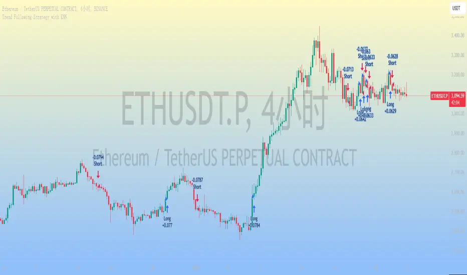
S&P 500 Benchmark Strategy
This strategy is a Benchmark Trend trading strategy. I used it primarily to measure my private algorithms against. It works on a variety of instruments at intervals between 1m and 1d (you'll have to play with some of the ranged variables in these cases). It was primarily designed to trade the 15 minute interval on SPX derived products. S&P E-Mini contract featured above.
It hits what I consider to be key targets when developing an algo:
1. Avg Trade is above $50
2. Profit Factor is above 1.2 (preferably above 1.5)
3. Has a relatively small draw-down
4. Is able to be traded both long and short
Notes/Options:
Can trade within market hours (default), outside market hours (with open inside), or anytime
Can adjust lengths for trend calculations
Algo tries its best to avoid fake-outs by using a volume component, this means that it misses 'slow rises' sometimes
By default it tries to only enter trades between 0930 and 1600. If the trade has left the station, it will wait for the next setup.
Stop loss level has a big impact on performance per instrument - default is 20 ticks but this has to be changed per instrument (I plan on updating this with code to auto-magically generate appropriate stop levels
As a Trend Following algorithm, it is vulnerable to chop zones but has been particularly resilient over the past few months when traded at 15m or 1h intervals. It is designed to trade against the 'current' market that has more frequent whipsaws. When used over generic bull market periods, it fails due to the high number of failed short trades and trimmed long trades. It works in a medium/high volatility environment.

Fusion Trend Pulse V2SCRIPT TITLE
Adaptive Fusion Trend Pulse V2 - Multi-Regime Strategy
DETAILED DESCRIPTION FOR PUBLICATION
🚀 INNOVATION SUMMARY
The Adaptive Fusion Trend Pulse V2 represents a breakthrough in algorithmic trading by introducing real-time market regime detection that automatically adapts strategy parameters based on current market conditions. Unlike static indicator combinations, this system dynamically adjusts its behavior across trending, choppy, and volatile market environments, providing a sophisticated multi-layered approach to market analysis.
🎯 CORE INNOVATIONS JUSTIFYING PROTECTED STATUS
1. Adaptive Market Regime Engine
Trending Market Detection: Uses ADX >25 with directional movement analysis
Volatile Market Classification: ATR-based volatility regime scoring (>1.2 threshold)
Choppy Market Identification: ADX <20 combined with volatility patterns
Dynamic Parameter Adjustment: All thresholds adapt based on detected regime
2. Multi-Component Fusion Algorithm
McGinley Dynamic Trend Baseline: Self-adjusting moving average that adapts to price velocity
Adaptive RMI (Relative Momentum Index): Enhanced RSI with momentum period adaptation
Zero-Lag EMA Smoothed CCI: Custom implementation reducing lag while maintaining signal quality
Hull MA Gradient Analysis: Slope strength normalized by ATR for trend confirmation
Volume Spike Detection: Regime-adjusted volume confirmation (0.8x-1.3x multipliers)
3. Intelligence Layer Features
Cooldown System: Prevents overtrading with regime-specific waiting periods (1-3 bars)
Performance Tracking: Real-time adaptation based on recent trade outcomes
Multi-Exchange Alert Integration: JSON-formatted alerts for automated trading
Comprehensive Dashboard: 16-metric real-time performance monitoring
📊 TECHNICAL SPECIFICATIONS
Market Regime Detection Philosophy:
The system continuously monitors market structure through volatility analysis and directional strength measurements. Rather than applying fixed thresholds, it creates dynamic response profiles that adjust the strategy's sensitivity, timing, and filtering based on the current market environment.
Adaptive Parameter Concept:
All strategy components modify their behavior based on regime classification. Volume requirements become more or less stringent, momentum thresholds shift to match market character, and exit timing adjusts to prevent whipsaws in different market conditions.
Entry Conditions (Both Long/Short):
McGinley trend alignment (close vs trend line)
Hull MA slope confirmation with ATR-normalized strength
Adaptive CCI above/below regime-specific thresholds
RMI momentum confirmation (>50 for long, <50 for short)
Volume spike exceeding regime-adjusted threshold
Regime-specific additional filters
Exit Strategy:
Dual take-profit system (2% and 4% default, customizable)
Momentum weakness detection (CCI reversal)
Trend breakdown (close below/above McGinley line)
Regime-specific urgency multipliers for faster exits in choppy markets
🎛️ USER CUSTOMIZATION OPTIONS
Core Parameters:
RMI Length & Momentum periods
CCI smoothing length
McGinley Dynamic length
Hull MA period for gradient analysis
Volume spike detection (length & multiplier)
Take profit levels (separate for long/short)
Adaptive Settings:
Market regime detection period (21 bars default)
Adaptation period for performance tracking (60 bars)
Volatility adaptation toggle
Trend strength filtering toggle
Momentum sensitivity multiplier (0.5-2.0 range)
Dashboard & Alerts:
Dashboard position (4 corners)
Dashboard size (Small/Normal/Large)
Transparency settings (0-100%)
Custom alert messages for bot integration
Date range filtering
🏆 UNIQUE VALUE PROPOSITIONS
1. Market Intelligence: First Pine Script strategy to implement comprehensive regime detection with parameter adaptation - most strategies use static settings regardless of market conditions.
2. Fusion Methodology: Combines 5+ distinct technical approaches (trend-following, momentum, volatility, volume, regime analysis) in a cohesive adaptive framework rather than simple indicator stacking.
3. Performance Optimization: Built-in learning system tracks recent performance and adjusts sensitivity - providing evolution rather than static rule-following.
4. Professional Integration: Enterprise-ready with JSON alert formatting, multi-exchange compatibility, and comprehensive performance tracking suitable for institutional use.
5. Visual Intelligence: Advanced dashboard provides 16 real-time metrics including regime classification, signal strength, and performance analytics - far beyond basic P&L displays.
🔧 TECHNICAL IMPLEMENTATION HIGHLIGHTS
Primary Applications:
Swing Trading: 4H-1D timeframes with regime-adapted entries
Algorithmic Trading: Automated execution via webhook alerts
Portfolio Management: Multi-timeframe analysis across different market conditions
Risk Management: Regime-aware position sizing and exit timing
Target Markets:
Cryptocurrency pairs (high volatility adaptation)
Forex majors (trending market optimization)
Stock indices (choppy market handling)
Commodities (volatile regime management)
🎯 WHY THIS ISN'T JUST AN INDICATOR MASHUP
Integrated Adaptation Framework: Unlike scripts that simply combine multiple indicators with static settings, this system creates a unified intelligence layer where each component influences and adapts to the others. The McGinley trend baseline doesn't just provide signals - it dynamically adjusts its sensitivity based on market regime detection. The momentum components modify their thresholds based on trend strength analysis.
Feedback Loop Architecture: The strategy incorporates a closed-loop learning system where recent performance influences future parameter selection. This creates evolution rather than static rule application. Most indicator combinations lack this adaptive learning capability.
Contextual Decision Making: Rather than treating each signal independently, the system uses contextual analysis where the same technical setup may generate different responses based on the current market regime. A momentum signal in a trending market triggers different behavior than the identical signal in choppy conditions.
Unified Risk Management: The regime detection doesn't just affect entries - it creates a comprehensive risk framework that adjusts exit timing, cooldown periods, and position management based on market character. This holistic approach distinguishes it from simple indicator stacking.
Custom Implementation Depth: Each component uses proprietary implementations (custom McGinley calculation, zero-lag CCI smoothing, enhanced RMI) rather than standard built-in functions, creating a cohesive algorithmic ecosystem rather than disconnected indicator outputs.
Custom Functions:
mcginley(): Proprietary implementation of McGinley Dynamic MA
rmi(): Enhanced Relative Momentum Index with custom parameters
zlema(): Zero-lag EMA for CCI smoothing
Regime classification algorithms with multi-factor analysis
Performance Optimizations:
Efficient variable management with proper scoping
Minimal repainting through careful historical referencing
Optimized calculations to prevent timeout issues
Memory-efficient tracking systems
Alert System:
JSON-formatted messages for API integration
Dynamic symbol/exchange substitution
Separate entry/exit/TP alert conditions
Customizable message formatting
⚡ WHY THIS REQUIRES PROTECTION
This strategy represents months of research into adaptive trading systems and market regime analysis. The specific combination of:
Proprietary regime detection algorithms
Custom adaptive parameter calculations
Multi-indicator fusion methodology
Performance-based learning system
Professional-grade implementation
Creates intellectual property that provides genuine competitive advantage. The methodology is not available in existing open-source scripts and represents original research into algorithmic trading adaptation.
🎯 EDUCATIONAL VALUE
Users gain exposure to:
Advanced market regime analysis techniques
Adaptive parameter optimization concepts
Multi-timeframe indicator fusion
Professional strategy development practices
Automated trading integration methods
The comprehensive dashboard and parameter explanations serve as a learning tool for understanding how professional algorithms adapt to changing market conditions.
CATEGORY SELECTION
Primary: Strategy
Secondary: Trend Analysis
SUGGESTED TAGS
adaptive, trend, momentum, regime, strategy, alerts, dashboard, mcginley, rmi, cci, professional
MANDATORY DISCLAIMER
Disclaimer: This strategy is for educational and informational purposes only. It does not constitute financial advice. Trading cryptocurrencies involves substantial risk, and past performance is not indicative of future results. Always backtest and forward-test before using on a live account. Use at your own risk.

Multi-Timeframe Wolfe Wave StrategyThis invite-only strategy implements an advanced multi-timeframe Wolfe Wave pattern recognition system specifically designed for institutional-grade algorithmic trading environments.
**Core Mathematical Framework:**
The strategy employs sophisticated mathematical calculations across 10 distinct timeframes (377, 233, 144, 89, 55, 34, 21, 13, 8, 5 periods), utilizing Elliott Wave ratio theory combined with proprietary algorithmic enhancements. Unlike standard Wolfe Wave implementations that rely on visual pattern recognition, this system uses quantitative analysis to identify precise entry and exit points.
**Technical Implementation:**
• **Pattern Detection Algorithm:** Calculates price relationships using configurable ratio sets including Fibonacci sequences, Elliott Wave ratios, Golden Ratio, Harmonic Patterns, Pi-based calculations, and custom mathematical progressions
• **Multi-Timeframe Confluence:** Simultaneously analyzes patterns across all timeframes to ensure signal reliability and reduce false positives
• **Dynamic Target Calculation:** Employs advanced mathematical modeling to project optimal profit targets based on historical price behavior and pattern completion theory
• **Risk Management Engine:** Implements position-based stop losses calculated as percentages of target profits, with liquidation price monitoring for leveraged positions
**Originality and Innovation:**
This implementation differs significantly from traditional Wolfe Wave indicators through several key innovations:
1. **Algorithmic Pattern Validation:** Uses mathematical confirmation across multiple timeframes rather than subjective visual analysis
2. **Adaptive Ratio Selection:** Offers 24 different ratio calculation methods, allowing optimization for various market conditions
3. **Institutional Integration:** Features comprehensive webhook messaging for automated execution via external trading systems
4. **Advanced Position Management:** Includes sophisticated position sizing controls with maximum concurrent position limits
**Strategy Logic:**
For bullish conditions, the algorithm identifies when price action meets specific mathematical criteria:
- Point validation through ratio analysis between swing highs/lows
- Confluence confirmation across multiple timeframes
- Minimum profit threshold filtering to ensure trade quality
- Dynamic stop-loss positioning based on pattern geometry
The mathematical approach uses proprietary calculations that extend beyond traditional Fibonacci levels, incorporating elements from chaos theory, fractal geometry, and advanced statistical analysis.
**Risk Management Features:**
• Configurable stop-loss percentages relative to profit targets
• Maximum position limits to control portfolio exposure
• Liquidation price monitoring for margin trading
• Time-based filtering options for market session control
• Minimum profit threshold settings to filter low-quality signals
**Intended Markets and Conditions:**
Optimized for cryptocurrency markets with high volatility and sufficient liquidity. Works effectively in trending and ranging market conditions due to its multi-timeframe approach. Best suited for assets with clear swing structure and adequate price movement.
**Performance Characteristics:**
The strategy is designed for active trading with frequent position entries across multiple timeframes. Position holding periods vary from short-term scalping to medium-term swing trading depending on pattern completion timeframes.
**Technical Requirements:**
Requires understanding of advanced pattern recognition theory, risk management principles, and algorithmic trading concepts. Users should be familiar with Wolfe Wave methodology and Elliott Wave theory fundamentals.

Flux Charts - SFX Automation💎 GENERAL OVERVIEW
The SFX Automation is a powerful and versatile tool designed to help traders rigorously test their trading strategies against historical market data. With various advanced settings, traders can fine-tune their strategies, assess performance, and identify key improvements before deploying in live trading environments. This tool offers a wide range of configurable settings, explained within this write-up.
Features of the new SFX Automation :
Step By Step : Configure your strategy step by step, which will allow you to have OR & AND logic in your strategies.
Highly Configurable : Offers multiple parameters for fine-tuning trade entry and exit conditions.
Multi-Timeframe Analysis : Allows traders to analyze multiple timeframes simultaneously for enhanced accuracy.
Provides advanced stop-loss, take-profit, and break-even settings.
Incorporates Buy & Sell signals, with settings like Signal Sensitivity, Strength, Time Weighting, Dynamic TP & SL Methods and more for refined strategy execution.
🚩 UNIQUENESS
The SFX Automation stands out from conventional backtesting tools due to its unparalleled flexibility, precision, and advanced trading logic integration. Key factors that make it unique include:
✅ Comprehensive Strategy Customization – Unlike traditional backtesters that offer basic entry and exit conditions, SFX Automation provides a highly detailed parameter set, allowing traders to fine-tune their strategies with precision.
✅ Multi-Timeframe Signals – This is the first-ever tool that allows traders to backtest Buy & Sell Signals on multiple timeframes.
✅ Customizable Take-Profit Conditions – Offers various methods to set take-profit exits, including using core features from SFX Algo, and dynamic exits like signal rating upgrades/downgrades, enabling traders to tailor their exit strategies to specific market behaviors.
✅ Customizable Stop-Loss Conditions – Provides several ways to set up stop losses, including using concepts from SFX Algo and trailing stops or dynamic exits like signal rating upgrades/downgrades, allowing for dynamic risk management tailored to individual strategies.
✅ Integration of External Indicators – Allows the inclusion of other indicators or data sources from TradingView for creating strategy conditions, enabling traders to enhance their strategies with additional insights and data points.
By integrating these advanced features, SFX Automation ensures that traders can rigorously test and optimize their strategies with great accuracy and efficiency.
📌 HOW DOES IT WORK ?
The first setting you will want to set it the pyramiding setting. This setting controls the number of simultaneous trades in the same direction allowed in the strategy. For example, if you set it to 1, only one trade can be active in any time, and the second trade will not be entered unless the first one is exited. If it is set to 2, the script will handle both of them at the same time. Note that you should enter the same value to this pyramiding setting, and the pyramiding setting in the "Properties" tab of the script for this to work.
You can enable and set a backtesting window that will limit the entries to between the start date & end date.
Entry Conditions
From the "Long Conditions" or the "Short Conditions" groups, you can set your position entry conditions. For settings like "initial capital" or "order size", you can open the "Properties" tab, where these are handled.
The SFX Algo can use the following conditions for entry conditions :
1. Buy Signal (Any, or 1-5 ☆)
This condition is triggered when a Buy Signal occurs. Other timeframes are supported with this condition.
2. Buy | TP (1, 2 or 3)
This condition is triggered when a TP signal of any Buy signal occurs.
3. Buy | SL
This condition is triggered when a SL signal of any Buy signal occurs.
4. Buy | Rating Upgrade
This condition is triggered when the rating of a buy signal is increased.
5. Buy | Rating Downgrade
This condition is triggered when the rating of a buy signal is decreased.
6. Sell Signal (Any, or 1-5 ☆)
This condition is triggered when a Sell Signal occurs. Other timeframes are supported with this condition.
7. Sell | TP (1, 2 or 3)
This condition is triggered when a TP signal of any Sell signal occurs.
8. Sell | SL
This condition is triggered when a SL signal of any Sell signal occurs.
9. Sell | Rating Upgrade
This condition is triggered when the rating of a sell signal is increased.
10. Sell | Rating Downgrade
This condition is triggered when the rating of a sell signal is decreased.
11. Retracement Wave Retest (Bullish or Bearish)
A retest on the Retracement Wave occurs when the price temporarily moves against the prevailing trend, touching or entering the wave before continuing in the original trend direction. This retest serves as a confirmation that the wave is acting as dynamic support or resistance.
12. Retracement Wave Retracement (Bullish or Bearish)
A retracement on the Retracement Wave occurs when the price touches the wave, the condition is triggered immediately.
13. Volatility Bands Retest (Bullish or Bearish)
A retest of Volatility Bands occurs when the price initially moves beyond the bands, then pulls back to "retest" the band it just broke through before continuing its move. This can provide traders with confirmation of a breakout or signal a potential reversal.
14. Volatility Bands Retracement (Bullish or Bearish)
A retracement on the Volatility Bands occur when the price touches the band, the condition is triggered immediately.
🕒 TIMEFRAME CONDITIONS
The SFX Automation supports Multi-Timeframe (MTF) features for Buy & Sell signals. When setting an entry condition, you can also choose the timeframe.
External Conditions
Users can use external indicators on the chart to set entry conditions.
The second dropdown in the external condition settings allows you to choose a conditional operator to compare external outputs. Available options include:
Less Than or Equal To: <=
Less Than: <
Equal To: =
Greater Than: >
Greater Than or Equal To: >=
The position entry conditions work like this ;
Each side has 3 SFX Algo conditions and 2 Source conditions. Each condition can be enabled or disabled using the checkbox on the left side of them.
You can select which timeframe this condition should work on for Buy & Sell signals. If you select "Chart", the condition will work for the chart's current timeframe.
Lastly select the step of this condition from 1 to 6.
The Source Condition
The last condition on each side is a source condition that is different from the others. Using this condition, you can create your own logic using other indicators' outputs on your chart. For example, suppose that you have an EMA indicator in your chart. You can have the source condition to something like "EMA > high".
The Step System
Each condition has a step number, and conditions are in topological order based on them.
The conditions are executed step by step. This means the condition with step 2 cannot be executed before the condition with step 1 is executed.
Conditions with the same step numbers have "OR" logic. This means that if you have 2 conditions with step 3, the condition with step 4 can trigger after only one of the step 3 conditions is executed.
➕ OTHER ENTRY FEATURES
The SFX Automation allows traders to choose when to execute trades and when not to execute trades.
1. Only Take Trades
This setting lets users specify the time period when their strategy can open or execute trades.
2. Don't Take Trades
This setting lets users specify time periods when their strategy can't open or execute trades.
↩️ EXIT CONDITIONS
1. Exit on Opposite Signal
When enabled, a long position will close when short entry conditions are met, and a short position will close when long entry conditions are met.
2. Exit on Session End
When enabled, positions will be closed at the end of the trading session.
📈 TAKE PROFIT CONDITIONS
There are several methods available for setting take profit exits and conditions.
1. Entry Condition TP
Users can use entry conditions as triggers for take profit exits. This setting can be found under the long and short exit conditions.
2. Fixed TP
Users can set a fixed TP for exits. This setting can be found under the long and short exit conditions. Users can choose between the following:
Price: This method triggers a TP exit when price reaches a specified level. For example, if you set the Price TP to 10 and buy NASDAQ:TSLA at $190, the trade will automatically exit when the price reaches $200 ($190 + $10).
Ticks: This method triggers a TP exit when price moves a specified number of ticks.
Percentage (%): This method triggers a TP exit when price moves a specified percentage.
ATR: This method triggers a TP exit based on a specified multiple of the Average True Range (ATR).
🧩EXIT PERCENTAGES
For each 3 dynamic take-profit conditions, you can set the amount of the position to exit in terms of percentage. It's important to make sure that the total of the exit percentages are 100%.
📉 STOP LOSS CONDITIONS
There are several methods available for setting stop-loss exits and conditions.
1. Entry Condition SL
Users can use entry conditions as triggers for stop-loss exits. This setting can be found under the long and short exit conditions.
2. Fixed SL
Users can set a fixed SL for exits. This setting can be found under the long and short exit conditions. Users can choose between the following:
Price: This method triggers a SL exit when price reaches a specified level. For example, if you set the Price SL to 10 and buy NASDAQ:TSLA at $200, the trade will automatically exit when the price reaches $190 ($200 - $10).
Ticks: This method triggers a SL exit when price moves a specified number of ticks.
Percentage (%): This method triggers a SL exit when price moves a specified percentage.
ATR: This method triggers a SL exit based on a specified multiple of the Average True Range (ATR).
3. Trailing Stop
An explanation & example for the trailing stop feature is present on the write-up within the next section.
Exit conditions have the same logic of constructing conditions like the entry ones. You can construct a Take-Profit Condition & a Stop-Loss Condition. Note that the Take-Profit condition will only work if the position is in profit, regardless of if it's triggered or not. The same applies for the Stop-Loss condition, meaning that it will only work if the position is in loss.
You can also set a Fixed TP & Fixed SL based on the price movement after the position is entered. You have options like "Price", "Ticks", "%", or "Average True Range". For example, you can set a Fixed TP like "5%", and the position will be entered once it moves 5% up in a long position.
Trailing Stop
For the Fixed SL, you also have a "Trailing" stop option, which you can set it's activation level as well. The Trailing stop activation level and it's value are expressed in ticks. Check this scenerio for an example :
We have a ticker with a tick value of $1. Our Trailing Stop is set to 10 ticks, and the activation level is set to 30 ticks.
We buy 1 contract when the price is $100.
When the price becomes $110, we are in $10 (10 ticks) profit and the trailing stop is now activated.
The current price our stop's on is $110 - $30 (30 ticks), which is the level of $80.
The trailing stop will only move if the price moves up the highest high the price has been after we entered the position.
Let's suppose that price moves up $40 right after our trailing stop is activated. The price will now be $150, and our trailing stop will sit on $150 - $30 (30 ticks) = $120.
If the price is down the $120 level, our stop loss will be triggered.
There is also a "Hard SL" option designed for a backup stop-loss when trailing stops are enabled. You can enable & set this option and if the price goes down before our trailing stop even activates, the position will be exited.
You can also move stop-loss to the break-even (entry price of the position) after a certain profit is achieved using the last setting of the exit conditions. Note that for this to work, you will need to have a Fixed SL setup.
➕ OTHER EXIT FEATURES
1. Move Stop Loss to Breakeven
This setting allows the strategy to automatically move the SL to Breakeven (BE) when the position is in profit by a certain amount. Users can choose between the following:
Price: This method moves the SL to BE when price reaches a specified level.
Ticks: This method moves the SL to BE when price moves a specified number of ticks.
Percentage (%): This method moves the SL to BE when price moves a specified percentage.
ATR: This method moves the SL to BE when price moves a specified multiple of the Average True Range (ATR).
Example Entry Scenario
To give an example , check this scenario; out conditions are :
LONG CONDITIONS
Buy Signal Any☆, Step 1
Bullish R. Wave Retest, Step 2
Bullish V. Bands Retest, Step 2
open > close, Step 3
First, the strategy needs to detect a Buy Signal with any star rating in order to start working.
After it's detected, now it's looking for either a Bullish R. Wave Retest, or a Bullish V. Bands Retest to proceed to the next step, the reason for this is that they both have the same step number.
After one of them is detected, the strategy will consistently check candlesticks for the condition open > close. If a bullish candlestick occurs, a long position will be entered.
⏰ ALERTS
This indicator uses TradingView's strategy alert system. All entries and exits will be sent as an alert if configured. It's possible to further customize these alerts to your liking. For more information, check TradingView's strategy alert customization page: www.tradingview.com
⚙️ SETTINGS
1. Backtesting Settings
Pyramiding: Controls the number of simultaneous trades allowed in the strategy. This setting must have the same value that is entered on the script's properties tab on the settings pane.
Enable Custom Backtesting Period: Restricts backtesting to a specific date range.
Start & End Time Configuration: Define precise start and end dates for historical analysis.
2. Algorithm Settings
Sensitivity: The sensitivity setting is a key parameter that influences the number of signals the SFX Algo generates. By adjusting this parameter, you can control the frequency of signals produced by the algorithm.
Signal Strength: The Signal Strength setting filters signals based on their quality, allowing traders to focus on the most reliable opportunities. This feature helps traders balance the quantity and reliability of the algorithm’s signals to suit their trading strategy.
Time Weighting: The Time Weighting setting determines how the SFX Algo evaluates historical market data to generate signals.
a) Recent Trends
Focuses on the most recent movements for short-term analysis. This setting is good for scalpers and intraday traders who need to react quickly to market changes.
b) Mixed Trends
Balances recent and historical price movements for a comprehensive market view. This setting is well-suited for swing traders and those who want to capture medium-term opportunities by combining the benefits of short-term responsiveness with the reliability of long-term trends.
c) Long-term Trends
Relies on extended historical market data to identify broader market trends, making it an excellent choice for traders focused on long-term strategies.
Minimum Star Rating: The Minimum Star Rating setting allows you to filter signals based on their strength, showing only those that meet or exceed your chosen threshold. For instance, setting the minimum star rating to 3 ensures you only receive signals with a rating of 3 stars or higher.
3. Take Profit / Stop Loss Methods
Key Levels
The Key Levels method uses pivot points to set take profit and stop-loss levels. The TP and SL levels are shown when a new signal is generated.
Volatility Bands
This TP/SL method uses the Volatility Bands overlay to set dynamic TP and SL levels. These levels are not predetermined so they will not be shown in advance when a signal is generated.
Signal Rating
Sets take profit and stop-loss levels based on changes in a signal's rating strength. These levels are not predetermined so they will not be shown in advance when a signal is generated.
Auto Stop-Loss
The auto method can only be applied to the SL. The auto method allows the algorithm to detect SL automatically when a momentum shift is detected. You can adjust the risk tolerance of the Auto SL by adjusting the ‘Auto Risk Tolerance’ setting. You can choose between Low, Medium, and High. A high-risk tolerance will result in stop losses being triggered less often.
4. Entry Conditions for Long & Short Trades
Multiple Conditions (1-6): Configure up to six independent conditions per trade direction.
Timeframe Specification: Choose between timeframes for Buy & Sell signals.
Trade Execution Filters: Restrict trades within specific trading sessions.
5. Exit Conditions for Long & Short Trades
Exit on Opposite Signal: Automatically exit trades upon opposite trade conditions.
Exit on Session End: Closes all positions at the end of the trading session.
Multiple Take-Profit (TP) and Stop-Loss (SL) Configurations:
TP/SL based on % move, ATR, Ticks, or Fixed Price.
Hard SL option for additional risk control.
Move SL to BE (Break Even) after a certain profit threshold.

BTC 5 min SHBHilalimSB A Wedding Gift 🌙
What is HilalimSB🌙?
First of all, as mentioned in the title, HilalimSB is a wedding gift.
HilalimSB - Revealing the Secrets of the Trend
HilalimSB is a powerful indicator designed to help investors analyze market trends and optimize trading strategies. Designed to uncover the secrets at the heart of the trend, HilalimSB stands out with its unique features and impressive algorithm.
Hilalim Algorithm and Fixed ATR Value:
HilalimSB is equipped with a special algorithm called "Hilalim" to detect market trends. This algorithm can delve into the depths of price movements to determine the direction of the trend and provide users with the ability to predict future price movements. Additionally, HilalimSB uses its own fixed Average True Range (ATR) value. ATR is an indicator that measures price movement volatility and is often used to determine the strength of a trend. The fixed ATR value of HilalimSB has been tested over long periods and its reliability has been proven. This allows users to interpret the signals provided by the indicator more reliably.
ATR Calculation Steps
1.True Range Calculation:
+ The True Range (TR) is the greatest of the following three values:
1. Current high minus current low
2. Current high minus previous close (absolute value)
3. Current low minus previous close (absolute value)
2.Average True Range (ATR) Calculation:
-The initial ATR value is calculated as the average of the TR values over a specified period
(typically 14 periods).
-For subsequent periods, the ATR is calculated using the following formula:
ATRt=(ATRt−1×(n−1)+TRt)/n
Where:
+ ATRt is the ATR for the current period,
+ ATRt−1 is the ATR for the previous period,
+ TRt is the True Range for the current period,
+ n is the number of periods.
Pine Script to Calculate ATR with User-Defined Length and Multiplier
Here is the Pine Script code for calculating the ATR with user-defined X length and Y multiplier:
//@version=5
indicator("Custom ATR", overlay=false)
// User-defined inputs
X = input.int(14, minval=1, title="ATR Period (X)")
Y = input.float(1.0, title="ATR Multiplier (Y)")
// True Range calculation
TR1 = high - low
TR2 = math.abs(high - close )
TR3 = math.abs(low - close )
TR = math.max(TR1, math.max(TR2, TR3))
// ATR calculation
ATR = ta.rma(TR, X)
// Apply multiplier
customATR = ATR * Y
// Plot the ATR value
plot(customATR, title="Custom ATR", color=color.blue, linewidth=2)
This code can be added as a new Pine Script indicator in TradingView, allowing users to calculate and display the ATR on the chart according to their specified parameters.
HilalimSB's Distinction from Other ATR Indicators
HilalimSB emerges with its unique Average True Range (ATR) value, presenting itself to users. Equipped with a proprietary ATR algorithm, this indicator is released in a non-editable form for users. After meticulous testing across various instruments with predetermined period and multiplier values, it is made available for use.
ATR is acknowledged as a critical calculation tool in the financial sector. The ATR calculation process of HilalimSB is conducted as a result of various research efforts and concrete data-based computations. Therefore, the HilalimSB indicator is published with its proprietary ATR values, unavailable for modification.
The ATR period and multiplier values provided by HilalimSB constitute the fundamental logic of a trading strategy. This unique feature aids investors in making informed decisions.
Visual Aesthetics and Clear Charts:
HilalimSB provides a user-friendly interface with clear and impressive graphics. Trend changes are highlighted with vibrant colors and are visually easy to understand. You can choose colors based on eye comfort, allowing you to personalize your trading screen for a more enjoyable experience. While offering a flexible approach tailored to users' needs, HilalimSB also promises an aesthetic and professional experience.
Strong Signals and Buy/Sell Indicators:
After completing test operations, HilalimSB produces data at various time intervals. However, we would like to emphasize to users that based on our studies, it provides the best signals in 1-hour chart data. HilalimSB produces strong signals to identify trend reversals. Buy or sell points are clearly indicated, allowing users to develop and implement trading strategies based on these signals.
For example, let's imagine you wanted to open a position on BTC on 2023.11.02. You are aware that you need to calculate which of the buying or selling transactions would be more profitable. You need support from various indicators to open a position. Based on the analysis and calculations it has made from the data it contains, HilalimSB would have detected that the graph is more suitable for a selling position, and by producing a sell signal at the most ideal selling point at 08:00 on 2023.11.02 (UTC+3 Istanbul), it would have informed you of the direction the graph would follow, allowing you to benefit positively from a 2.56% decline.
Technology and Innovation:
HilalimSB aims to enhance the trading experience using the latest technology. With its innovative approach, it enables users to discover market opportunities and support their decisions. Thus, investors can make more informed and successful trades. Real-Time Data Analysis: HilalimSB analyzes market data in real-time and identifies updated trends instantly. This allows users to make more informed trading decisions by staying informed of the latest market developments. Continuous Update and Improvement: HilalimSB is constantly updated and improved. New features are added and existing ones are enhanced based on user feedback and market changes. Thus, HilalimSB always aims to provide the latest technology and the best user experience.
Social Order and Intrinsic Motivation:
Negative trends such as widespread illegal gambling and uncontrolled risk-taking can have adverse financial effects on society. The primary goal of HilalimSB is to counteract these negative trends by guiding and encouraging users with data-driven analysis and calculable investment systems. This allows investors to trade more consciously and safely.
What is BTC 5 min ☆SHB Strategy🌙?
BTC 5 min ☆SHB Strategy is a strategy supported by the HilalimSB algorithm created by the creator of HilalimSB. It automatically opens trades based on the data it receives, maintaining trades with its uniquely defined take profit and stop loss levels, and automatically closes trades when necessary. It stands out in the TradingView world with its unique take profit and stop loss markings. BTC 5 min ☆SHB Strategy is close to users' initiatives and is a strategy suitable for 5-minute trades and scalp operations developed on BTC.
What does the BTC 5 min ☆SHB Strategy target?
The primary goal of BTC 5 min ☆SHB Strategy is to close trades made by traders in short timeframes as profitably as possible and to determine the most effective trading points in low time periods, considering the commission rates of various brokerage firms. BTC 5 min ☆SHB Strategy is one of the rare profitable strategies released in short timeframes, with its useful interface, in addition to existing strategies in the markets. After extensive backtesting over a long period and achieving above-average success, BTC 5 min ☆SHB Strategy was decided to be released. Following the completion of test procedures under market conditions, it was presented to users with the unique visual effects of ☆SB.
BTC 5 min ☆SHB Strategy and Heikin Ashi
BTC 5 min ☆SHB Strategy produces data in Heikin-Ashi chart types, but since Heikin-Ashi chart types have their own calculation method, BTC 5 min ☆SHB Strategy has been published in a way that cannot produce data in this chart type due to BTC 5 min ☆SHB Strategy's ideology of appealing to all types of users, and any confusion that may arise is prevented in this way. Heikin-Ashi chart types, especially in short time intervals, carry significant risks considering the unique calculation methods involved. Thus, the possibility of being misled by the coder and causing financial losses has been completely eliminated. After the necessary conditions determined by the creator of BTC 5 min ☆SHB are met, BTC 5 min ☆SHB Heikin-Ashi will be shared exclusively with invited users only, upon request, to users who request an invitation.
Key Features:
+HilalimSHB Algorithm: This algorithm uses a dynamic ATR-based trend-following mechanism to identify the current market trend. The strategy detects trend reversals and takes positions accordingly.
+Heikin Ashi Compatibility: The strategy is optimized to work only with standard candlestick charts and automatically deactivates when Heikin Ashi charts are in use, preventing false signals.
+Advanced Chart Enhancements: The strategy offers clear graphical markers for buy/sell signals. Candlesticks are automatically colored based on trend direction, making market trends easier to follow.
Strategy Parameters:
+Take Profit (%): Defines the target price level for closing a position and automates profit-taking. The fixed value is set at 2%.
+Stop Loss (%): Specifies the stop-loss level to limit losses. The fixed value is set at 3%.
The shared image is a 5-minute chart of BTCUSDC.P with a fixed take profit value of 2% and a fixed stop loss value of 3%. The trades are opened with a commission rate of 0.063% set for the USDT trading pair on Binance.🌙
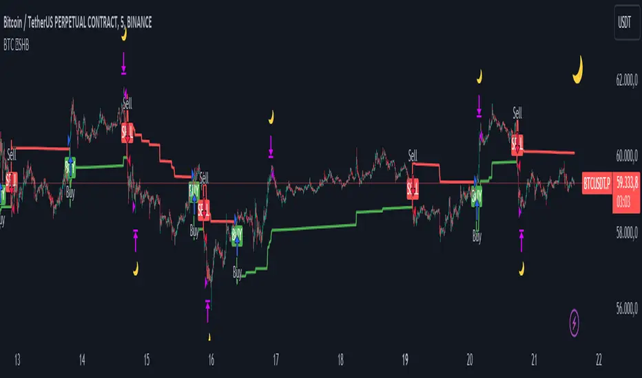
Crypto Punk [Bot] (Zeiierman)█ Overview
The Crypto Punk (Zeiierman) is a trading strategy designed for the dynamic and volatile cryptocurrency market. It utilizes algorithms that incorporate price action analysis and principles inspired by Geometric Brownian Motion (GBM). The bot's core functionality revolves around analyzing differences in high and low prices over various timeframes, estimating drift (trend) and volatility, and applying this information to generate trading signals.
█ How to use the Crypto Punk Bot
Utilize the Crypto Punk Bot as a technical analysis tool to enhance your trading strategy. The signals generated by the bot can serve as a confirmation of your existing approach to entering and exiting the market. Additionally, the backtest report provided by the bot is a valuable resource for identifying the optimal settings for the specific market and timeframe you are trading in.
One method is to use the bot's signals to confirm entry points around key support and resistance levels.
█ Key Features
Let's explain how the core features work in the strategy.
⚪ Strategy Filter
The strategy filter plays a vital role in the entries and exits. By setting this filter, the bot can identify higher or lower price points at which to execute trades. Opting for higher values will make the bot target more long-term extreme points, resulting in fewer but potentially more significant signals. Conversely, lower values focus on short-term extreme points, offering more frequent signals focusing on immediate market movements.
How is it calculated?
This filter identifies significant price points within a specified dynamic range by applying linear regression to the absolute deviation of the range, smoothing out fluctuations, and determining the trend direction. The algorithm then normalizes the data and searches for extreme points.
⚪ External AI filter
The external AI filter allows traders to incorporate two external sources as signal filters. This feature is particularly useful for refining their signal accuracy with additional data inputs.
External sources can include any indicator applied to your TradingView chart that produces a plot as an output, such as a moving average, RSI, supertrend, MACD, etc. Traders can use these indicators of their choice to set filters for screening signals within the strategy.
This approach offers traders increased flexibility to select filters that align with their trading style. For instance, one trader might prefer to take trades when the price is above a moving average, while another might opt for trades when the MACD is below the MACD signal line. These external filters enable traders to choose options that best fit their trading strategies. See the example below. Note that the input sources for the External AI filter can be any indicator applied to the chart, and the input source per se does not make this strategy unique. The AI filter takes the selected input source and applies our function to it. So, if a trader selects RSI as an input filter, RSI is not unique, but how the source is computed within the AI functions is.
How is it calculated?
Once the external filters are selected and enabled within the settings panel, our AI function is applied to enhance the filter's ability to execute trades, even when the set conditions of the filter are not met. For instance, if a trader wants to take trades only when the price is above a moving average, the AI filter can actually execute trades even if the price is below the moving average.
The filter works by combining k-nearest Neighbors (KNN) with Geometric Brownian Motion (GBM) involves first using GBM to model the historical price trends of an asset, identifying patterns of drift and volatility. KNN is then applied to compare the current market conditions with historical instances, identifying the closest matches based on similar market behaviors. By examining the drift values of these nearest historical neighbors, KNN predicts the current trend's direction.
The AI adaptability value is a setting that determines how flexible the AI algorithm is when applying the external AI filter. Setting the adaptability to 10 indicates minimal adaptability, suggesting that the bot will strictly adhere to the set filter criteria. On the other hand, a higher adaptability value grants the algorithm more leeway to "think outside the box," allowing it to consider signals that may not strictly meet the filter criteria but are deemed viable trading opportunities by the AI.
█ Examples
In this example, the RSI is used to filter out signals when the RSI is below the smoothing line, indicating that prices are declining.
Note that the external filter is specifically designed to work with either 'LONG ONLY' or 'SHORT ONLY' modes; it does not apply when the bot is set to trade on 'BOTH' modes. For 'LONG ONLY' positions, the filter criteria are met when source 1 is greater than source 2 (source 1 >= source 2). Conversely, for 'SHORT ONLY' positions, the filter criteria require source 1 to be less than source 2 (source 1 <= source 2).
Examples of Filter Usage:
Long Signals: To receive long signals when the closing price is higher than a moving average, set Source 1 to the 'close' price and Source 2 to a moving average value. This setup ensures that signals are generated only when the closing price exceeds the moving average, indicating a potential upward trend.
█ Settings
⚪ Set Timeframe
Choosing the correct entry and exit timeframes is crucial for the bot's performance. The general guideline is to select a timeframe that is higher than the one currently displayed on the trading chart but still relatively close in duration. For instance, if trading on a 1-minute chart, setting the bot's Timeframe to 5 minutes is advisable.
⚪ Entry
Traders have the flexibility to configure the bot according to their trading strategy, allowing them to choose whether the bot should engage in long positions only, short positions only or both. This customization ensures that the bot aligns with the trader's market outlook and risk tolerance.
⚪ Pyramiding
Pyramiding functionality is available to enhance the bot's trading strategy. If the current position experiences a drawdown by a specified number of points, the bot is programmed to add new positions to the existing one, potentially capitalizing on lower prices to average down the entry cost. To utilize this feature, access the settings panel, navigate to 'Properties,' and look for 'Pyramiding' to specify the number of times the bot can re-enter the market (e.g., setting it to 2 allows for two additional entries).
⚪ Risk Management
The bot incorporates several risk management methods, including a regular stop loss, trailing stop, and risk-reward-based stop loss and exit strategies. These features assist traders in managing their risk.
Stop Loss
Trailing Stop
⚪ Trading on specific days
This feature allows trading on specific days by setting which days of the week the bot can execute trades on. It enables traders to tailor their strategies according to market behavior on particular days.
⚪ Alerts
Alerts can be set for entry, exit, and risk management. This feature allows traders to automate their trading strategy, ensuring timely actions are taken according to predefined criteria.
█ How is Crypto Punk calculated?
The Crypto Punk Bot is a trading bot that utilizes a combination of price action analysis and elements inspired by Geometric Brownian Motion (GBM) to generate buy and sell signals for cryptocurrencies. The bot focuses on analyzing the difference between high and low prices over various timeframes, alongside estimates of drift (trend) and volatility derived from GBM principles.
Timeframe Analysis for Price Action
The bot examines multiple timeframes (e.g., daily, weekly) to identify the range between the highest and lowest prices within each period. This range analysis helps in understanding market volatility and the potential for significant price movements. The algorithm calculates the trading range by applying maximum and minimum functions to the set of prices over your selected timeframe. It then subtracts these values to determine the range's width. This method offers a quantitative measure of the asset's price volatility for the specified period.
Estimating Drift (Trend)
The bot estimates the drift component, which reflects the underlying trend or expected return of the cryptocurrency. The algorithm does this by estimating the drift (trend) using Geometric Brownian Motion (GBM), which involves determining an asset's average rate of return over time, reflecting the asset's expected direction of movement.
Estimating Volatility
Volatility is estimated by calculating the standard deviation of the logarithmic returns of the cryptocurrency's price over the same timeframe used for the drift calculation. Geometric Brownian Motion (GBM) involves measuring the extent of variation or dispersion in the returns of an asset over time. In the context of GBM, volatility quantifies the degree to which the price of an asset is expected to fluctuate around its drift.
Combining Drift and Volatility for Signal Generation
The bot uses the calculated drift and volatility to understand the current market conditions. A higher drift coupled with manageable volatility may indicate a strong upward trend, suggesting a potential buy signal. Conversely, a low or negative drift with increasing volatility might suggest a weakening market, triggering a sell signal.
█ Strategy Properties
This script backtest is done on the 1 hour chart Bitcoin, using the following backtesting properties:
Balance (default): 10 000 (default base currency)
Order Size: 10% of the equity
Commission: 0.05 %
Slippage: 500 ticks
Stop Loss: Risk Reward set to 1
These parameters are set to provide an accurate representation of the backtesting environment. It's important to recognize that default settings may vary for several reasons outlined below:
Order Size: The standard is set at one contract to facilitate compatibility with a wide range of instruments, including futures.
Commission: This fee is subject to fluctuation based on the specific market and financial instrument, and as such, there isn't a standard rate that will consistently yield accurate outcomes.
We advise users to customize the Script Properties in the strategy settings to match their personal trading accounts and preferred platforms. This adjustment is crucial for obtaining practical insights from the deployed strategies.
-----------------
Disclaimer
The information contained in my Scripts/Indicators/Ideas/Algos/Systems does not constitute financial advice or a solicitation to buy or sell any securities of any type. I will not accept liability for any loss or damage, including without limitation any loss of profit, which may arise directly or indirectly from the use of or reliance on such information.
All investments involve risk, and the past performance of a security, industry, sector, market, financial product, trading strategy, backtest, or individual's trading does not guarantee future results or returns. Investors are fully responsible for any investment decisions they make. Such decisions should be based solely on an evaluation of their financial circumstances, investment objectives, risk tolerance, and liquidity needs.
My Scripts/Indicators/Ideas/Algos/Systems are only for educational purposes!
Paid script