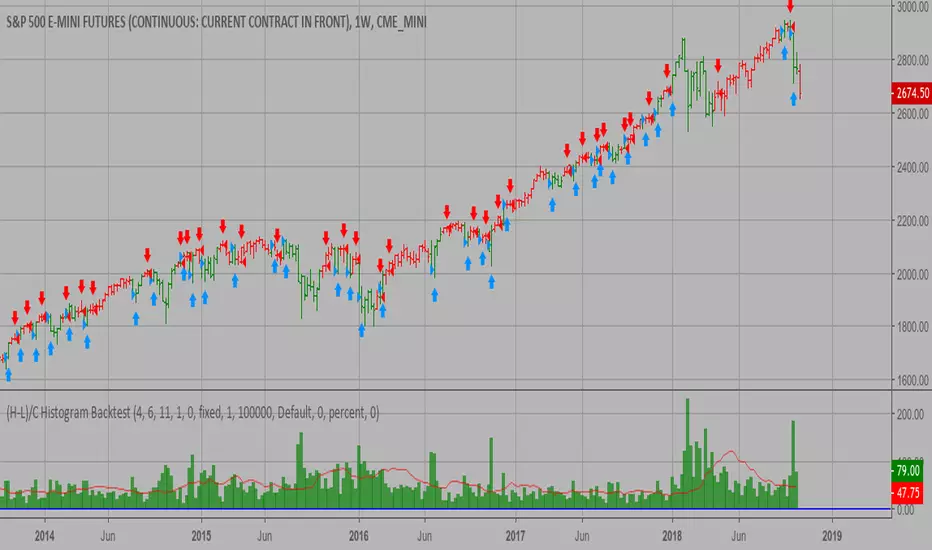
(H-L)/C Histogram Backtest This histogram displays (high-low)/close
Can be applied to any time frame.
WARNING:
- For purpose educate only
- This script to change bars colors.
Cari dalam skrip untuk "backtest"
CMO & WMA Backtest ver 2.0 This indicator plots Chandre Momentum Oscillator and its WMA on the
same chart. This indicator plots the absolute value of CMO.
The CMO is closely related to, yet unique from, other momentum oriented
indicators such as Relative Strength Index, Stochastic, Rate-of-Change,
etc. It is most closely related to Welles Wilder?s RSI, yet it differs
in several ways:
- It uses data for both up days and down days in the numerator, thereby
directly measuring momentum;
- The calculations are applied on unsmoothed data. Therefore, short-term
extreme movements in price are not hidden. Once calculated, smoothing
can be applied to the CMO, if desired;
- The scale is bounded between +100 and -100, thereby allowing you to clearly
see changes in net momentum using the 0 level. The bounded scale also allows
you to conveniently compare values across different securities.

Trend Trader Bands Backtest This is plots the indicator developed by Andrew Abraham
in the Trading the Trend article of TASC September 1998
It was modified, result values wass averages.
And draw two bands above and below TT line.

Ichimoku Backtest Ichimoku Strategy
You can change long to short in the Input Settings
WARNING:
- For purpose educate only
- This script to change bars colors.

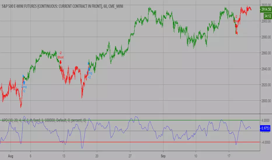
Absolute Price Oscillator (APO) Backtest 2.0 The Absolute Price Oscillator displays the difference between two exponential
moving averages of a security's price and is expressed as an absolute value.
How this indicator works
APO crossing above zero is considered bullish, while crossing below zero is bearish.
A positive indicator value indicates an upward movement, while negative readings
signal a downward trend.
Divergences form when a new high or low in price is not confirmed by the Absolute Price
Oscillator (APO). A bullish divergence forms when price make a lower low, but the APO
forms a higher low. This indicates less downward momentum that could foreshadow a bullish
reversal. A bearish divergence forms when price makes a higher high, but the APO forms a
lower high. This shows less upward momentum that could foreshadow a bearish reversal.
You can change long to short in the Input Settings
WARNING:
- For purpose educate only
- This script to change bars colors.
Keltner Channel Backtest The Keltner Channel, a classic indicator
of technical analysis developed by Chester Keltner in 1960.
The indicator is a bit like Bollinger Bands and Envelopes.
You can change long to short in the Input Settings
WARNING:
- For purpose educate only
- This script to change bars colors.

Volatility Backtest The Volatility function measures the market volatility by plotting a
smoothed average of the True Range. It returns an average of the TrueRange
over a specific number of bars, giving higher weight to the TrueRange of
the most recent bar.
You can change long to short in the Input Settings
WARNING:
- For purpose educate only
- This script to change bars colors.

Smart Money Index (SMI) Backtest Attention:
If you would to use this indicator on the ES, you should have intraday data 60min in your account.
Smart money index (SMI) or smart money flow index is a technical analysis indicator demonstrating investors sentiment.
The index was invented and popularized by money manager Don Hays. The indicator is based on intra-day price patterns.
The main idea is that the majority of traders (emotional, news-driven) overreact at the beginning of the trading day
because of the overnight news and economic data. There is also a lot of buying on market orders and short covering at the opening.
Smart, experienced investors start trading closer to the end of the day having the opportunity to evaluate market performance.
Therefore, the basic strategy is to bet against the morning price trend and bet with the evening price trend. The SMI may be calculated
for many markets and market indices (S&P 500, DJIA, etc.)
The SMI sends no clear signal whether the market is bullish or bearish. There are also no fixed absolute or relative readings signaling
about the trend. Traders need to look at the SMI dynamics relative to that of the market. If, for example, SMI rises sharply when the
market falls, this fact would mean that smart money is buying, and the market is to revert to an uptrend soon. The opposite situation
is also true. A rapidly falling SMI during a bullish market means that smart money is selling and that market is to revert to a downtrend
soon. The SMI is, therefore, a trend-based indicator.
Some analysts use the smart money index to claim that precious metals such as gold will continually maintain value in the future.
You can change long to short in the Input Settings
WARNING:
- For purpose educate only
- This script to change bars colors.

High and Low Levels Backtest This script shows a high and low period value.
Width - width of lines
SelectPeriod - Day or Week or Month and etc.
LookBack - Shift levels 0 - current period, 1 - previous and etc.
You can change long to short in the Input Settings
WARNING:
- For purpose educate only
- This script to change bars colors.

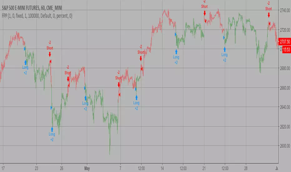
Floor Pivot Points Backtest The name ‘Floor-Trader Pivot,’ came from the fact that Pivot points can
be calculated quickly, on the fly using price data from the previous day
as an input. Although time-frames of less than a day can be used, Pivots are
commonly plotted on the Daily Chart; using price data from the previous day’s
trading activity.
You can change long to short in the Input Settings
WARNING:
- For purpose educate only
- This script to change bars colors.
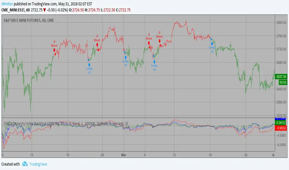
CMOaDisparity Index Backtest The related article is copyrighted materialfrom Stocks & Commodities Dec 2009
My strategy modification.
You can change long to short in the Input Settings
WARNING:
- For purpose educate only
- This script to change bars colors.
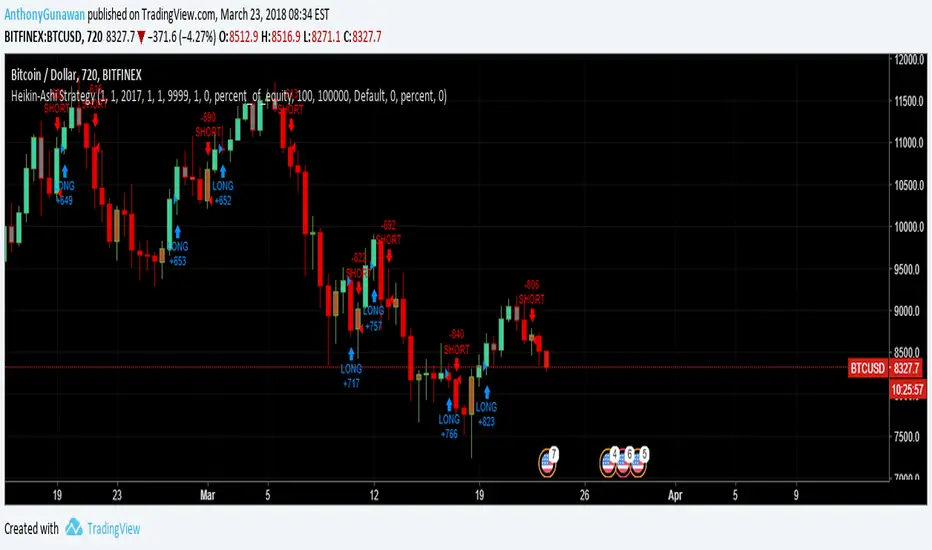
Heikin-Ashi Strategy + backtest rangeThis is Heikin-Ashi Strategy + Backtest range that I think useful for BTCUSD pair.
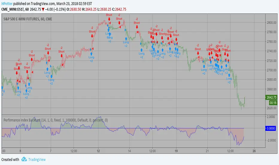
Perfomance index Backtest The Performance indicator or a more familiar term, KPI (key performance indicator),
is an industry term that measures the performance. Generally used by organizations,
they determine whether the company is successful or not, and the degree of success.
It is used on a business’ different levels, to quantify the progress or regress of a
department, of an employee or even of a certain program or activity. For a manager
it’s extremely important to determine which KPIs are relevant for his activity, and
what is important almost always depends on which department he wants to measure the
performance for. So the indicators set for the financial team will be different than
the ones for the marketing department and so on.
Similar to the KPIs companies use to measure their performance on a monthly, quarterly
and yearly basis, the stock market makes use of a performance indicator as well, although
on the market, the performance index is calculated on a daily basis. The stock market
performance indicates the direction of the stock market as a whole, or of a specific stock
and gives traders an overall impression over the future security prices, helping them decide
the best move. A change in the indicator gives information about future trends a stock could
adopt, information about a sector or even on the whole economy. The financial sector is the
most relevant department of the economy and the indicators provide information on its overall
health, so when a stock price moves upwards, the indicators are a signal of good news. On the
other hand, if the price of a particular stock decreases, that is because bad news about its
performance are out and they generate negative signals to the market, causing the price to go
downwards. One could state that the movement of the security prices and consequently, the movement
of the indicators are an overall evaluation of a country’s economic trend.
You can change long to short in the Input Settings
WARNING:
- For purpose educate only
- This script to change bars colors.
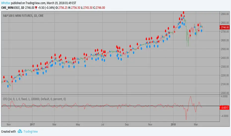
Chande Forecast Oscillator Backtest The Chande Forecast Oscillator developed by Tushar Chande The Forecast
Oscillator plots the percentage difference between the closing price and
the n-period linear regression forecasted price. The oscillator is above
zero when the forecast price is greater than the closing price and less
than zero if it is below.
You can change long to short in the Input Settings
WARNING:
- For purpose educate only
- This script to change bars colors.
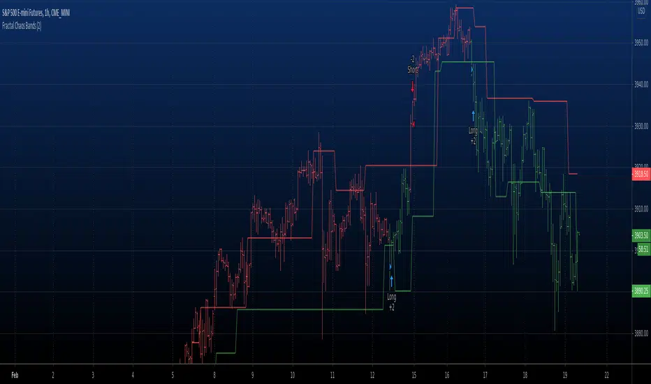
Fractal Chaos Bands Backtest The FCB indicator looks back in time depending on the number of time periods trader selected
to plot the indicator. The upper fractal line is made by plotting stock price highs and the
lower fractal line is made by plotting stock price lows. Essentially, the Fractal Chaos Bands
show an overall panorama of the price movement, as they filter out the insignificant fluctuations
of the stock price.
You can change long to short in the Input Settings
WARNING:
- For purpose educate only
- This script to change bars colors.
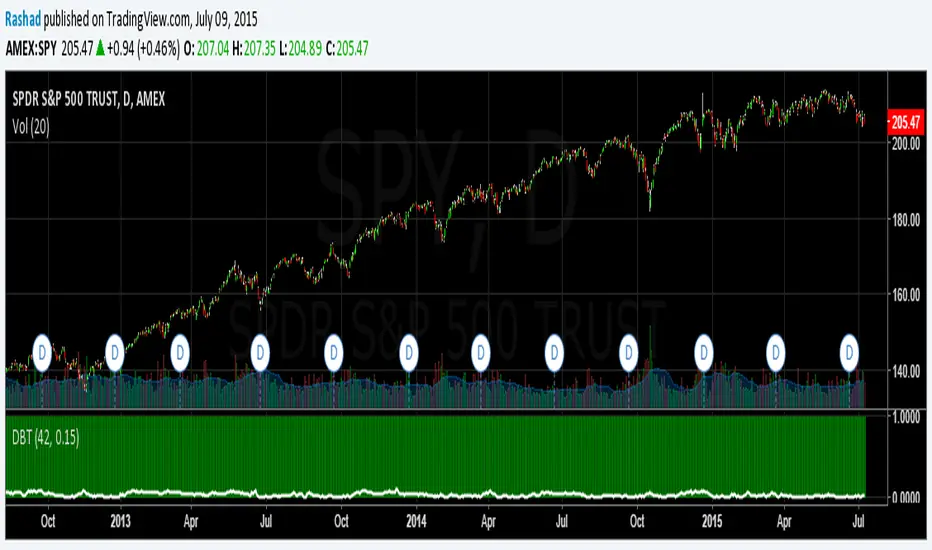
Deviation Back Tester (Great for Credit Spreads)!Error with math fixed in this one. Please use this one.
This is great for credit spreads! Lets say you wanted to know if you had sold a 15% OTM Bull Put vertical 2 months out, how often would you win? This Turns green if you would have been correct with your credit spread had it expired on that date, or red if you would've been wrong. Great for Back testing!
This could also be used for ATM debit spreads credit spreads etc. Example, how often does SPY deviate outside a 10% range relative to two months, 5% (if your doing straddles perhaps) etc.
This Can be used with any stock.
PLEASE KEEP IN MIND THAT IT TESTS DEVIATION IN BOTH DIRECTIONS. THEREFORE IT WILL HIGHLIGHT RED ON BOTH THE UPSIDE AND DOWNSIDE. WHEN BACKTESTING BE SURE TO CHECK WHETHER IT IS RED BECAUSE OF DOWNSIDE OR UPSIDE.
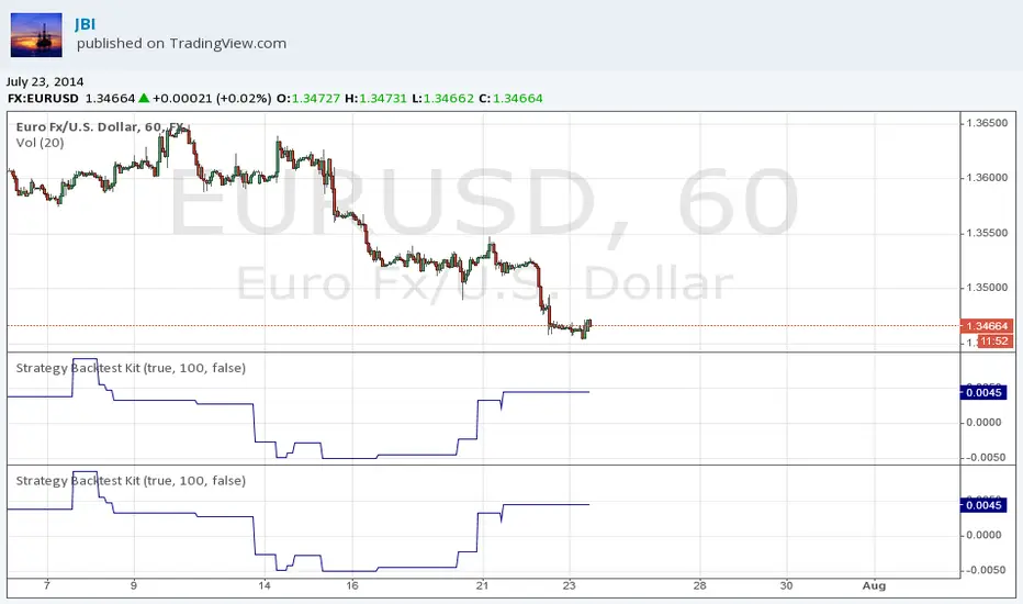
Strategy Backtest KitStrategy Backtest Kit. You have just to define your own entry / exit setups. The strategy I have coded into this is : BUY when MACD > 0 / SELL when MACD < 0. Always in position.
Follow JBI for his daily analyses!
Liquidity Sweep Detector - PDH/PDL LevelsPrevious Day High/Low Liquidity Sweep Detector (Intraday Accurate)
This indicator tracks the previous day's high and low using intraday data, rather than the daily candle, ensuring precise sweep detection across lower timeframes (15m to 4H).
It monitors for liquidity sweeps—moments when price briefly moves above the previous high or below the previous low—and visually marks these events on the chart.
Key Features
Intraday-accurate PDH/PDL tracking
Real-time sweep detection
On-chart labels marking sweep events
Toggleable table showing sweep status
Alert conditions for PDH/PDL sweep triggers
Best For
Traders who use Smart Money Concepts (SMC), liquidity-based strategies, or look for stop hunts and reversal zones tied to key prior-day levels.
Works well across FX, crypto, and indices on 15m, 1H, and 4H charts.

RSI MTF Ob+OsHello Traders,
This indicator use the same concept as my previous indicator "CCI MTF Ob+Os".
It is a simple "Relative Strength Index" ( RSI ) indicator with multi-timeframe (MTF) overbought and oversold level.
It can detect overbought and oversold level up to 5 timeframes, which help traders spot potential reversal point more easily.
There are options to select 1-5 timeframes to detect overbought and oversold.
Aqua Background is "Oversold" , looking for "Long".
Orange Background is "Overbought" , looking for "Short".
Have fun :)

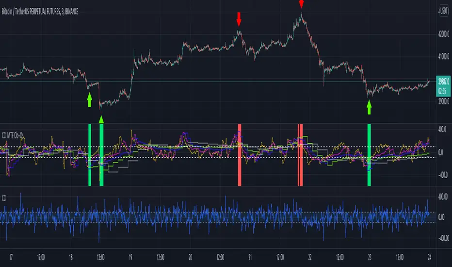
CCI MTF Ob+OsHello Traders,
This is a simple Commodity Channel Index (CCI) indicator with multi-timeframe (MTF) overbought and oversold level.
It can detect overbought and oversold level up to 5 timeframes, which help traders spot potential reversal point more easily.
There are options to select 1-5 timeframes to detect overbought and oversold.
Green Background is "Oversold" , looking for "Long".
Red Background is "Overbought" , looking for "Short".
Have fun :)
Demand & Supply Zones [eyes20xx]Demand & Supply Zones
This indicator helps to identify large moves driven by institutions.
What qualifies as a zone?
If the price moves (open to close) by more than a certain % in one candle or in a bullish / bearish run of candles, the zone is marked as a Demand or Supply zone .
0.8% is good for Crypto and Forex might be better with 0.4%. Play around with the % to match your requirements.
Active zones
A zone remains active until it is hit by the price. When it becomes inactive, the zone background becomes transparent.
Zone lines
Lines are displayed if the zone is active and within a certain % of the close. 3% is a good setting for Crypto.
A maximum of two lines are displayed for each zone type.

Simple Candle Info This script shows the following simple information about the last candle:
- Candle size
- Body size included %
- Top Wick size
- Bottom Wick size
- Top Wick + Body size
- Bottom Wick + Body size
You can change:
- colors and position for labels
- add information for previous candle too
- change language

Percentage Change FunctionThis is little code snippet can be copied and pasted into your own strategies and indicators to easily calculate some interesting percentage change levels within a given lookback period.
The function will return:
The price change from the start to the end of the period
The price change from the start of the period to the highest point within the period
The price change from the start of the period to the lowest point within the period
It was originally intended to be used in conjunction with other scripts to assist with decision making. However, it doesn't look too bad as an indicator and so plots have been added.
For more information regarding the code, some commentary and free tutorials, you can visit the Bactest-Rookies (.com) website.