Long Position with 1:3 Risk Reward and 20EMA CrossoverThe provided Pine Script code implements a strategy to identify long entry signals based on a 20-EMA crossover on a 5-minute timeframe. Once a buy signal is triggered, it calculates and plots the following:
Entry Price: The price at which the buy signal is generated.
Stop Loss: The low of the previous candle, acting as a risk management tool.
Take Profit: The price level calculated based on a 1:3 risk-reward ratio.
Key Points:
Buy Signal: A buy signal is generated when the current 5-minute candle closes above the 20-EMA.
Risk Management: The stop-loss is set below the entry candle to limit potential losses.
Profit Target: The take-profit is calculated based on a 1:3 risk-reward ratio, aiming for a potential profit three times the size of the risk.
Visualization: The script plots the entry price, stop-loss, and take-profit levels on the chart for visual clarity.
Remember:
Backtesting: It's crucial to backtest this strategy on historical data to evaluate its performance and optimize parameters.
Risk Management: Always use appropriate risk management techniques, such as stop-loss orders and position sizing, to protect your capital.
Market Conditions: Market conditions can change, and strategies that worked in the past may not perform as well in the future. Continuously monitor and adapt your strategy.
By understanding the core components of this script and applying sound risk management principles, you can effectively use it to identify potential long entry opportunities in the market.
Cari dalam skrip untuk "backtest"

[blackcat] L1 Simple Dual Channel Breakout█ OVERVIEW
The script " L1 Simple Dual Channel Breakout" is an indicator designed to plot dual channel breakout bands and their long-term EMAs on a chart. It calculates short-term and long-term moving averages and deviations to establish upper, lower, and middle bands, which traders can use to identify potential breakout opportunities.
█ LOGICAL FRAMEWORK
Structure:
The script is structured into several main sections:
• Input Parameters: The script does not explicitly define input parameters for the user to adjust, but it uses default values for short_term_length (5) and long_term_length (181).
• Calculations: The calculate_dual_channel_breakout function performs the core calculations, including the blast condition, typical price, short-term and long-term moving averages, and dynamic moving averages.
• Plotting: The script plots the short-term bands (upper, lower, and middle) and their long-term EMAs. It also plots conditional line breaks when the short-term bands cross the long-term EMAs.
Flow of Data and Logic:
1 — The script starts by defining the calculate_dual_channel_breakout function.
2 — Inside the function, it calculates various moving averages and deviations based on the input prices and lengths.
3 — The function returns the calculated bands and EMAs.
4 — The script then calls this function with predefined lengths and plots the resulting bands and EMAs on the chart.
5 — Conditional plots are added to highlight breakouts when the short-term bands cross the long-term EMAs.
█ CUSTOM FUNCTIONS
The script defines one custom function:
• calculate_dual_channel_breakout(close_price, high_price, low_price, short_term_length, long_term_length): This function calculates the short-term and long-term bands and EMAs. It takes five parameters: close_price, high_price, low_price, short_term_length, and long_term_length. It returns an array containing the upper band, lower band, middle band, long-term upper EMA, long-term lower EMA, and long-term middle EMA.
█ KEY POINTS AND TECHNIQUES
• Typical Price Calculation: The script uses a modified typical price calculation (2 * close_price + high_price + low_price) / 4 instead of the standard (high_price + low_price + close_price) / 3.
• Short-term and Long-term Bands: The script calculates short-term bands using a simple moving average (SMA) of the typical price and long-term bands using a relative moving average (RMA) of the close price.
• Conditional Plotting: The script uses conditional plotting to highlight breakouts when the short-term bands cross the long-term EMAs, enhancing visual identification of trading signals.
• EMA for Long-term Trends: The use of Exponential Moving Averages (EMAs) for long-term bands helps in smoothing out short-term fluctuations and focusing on long-term trends.
█ EXTENDED KNOWLEDGE AND APPLICATIONS
• Modifications: Users can add input parameters to allow customization of short_term_length and long_term_length, making the indicator more flexible.
• Enhancements: The script could be extended to include alerts for breakout conditions, providing traders with real-time notifications.
• Alternative Bands: Users might experiment with different types of moving averages (e.g., WMA, HMA) for the short-term and long-term bands to see if they yield better results.
• Additional Indicators: Combining this indicator with other technical indicators (e.g., RSI, MACD) could provide a more comprehensive trading strategy.
• Backtesting: Users can backtest the strategy using Pine Script's strategy functions to evaluate its performance over historical data.

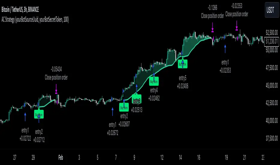
MultiLayer Acceleration/Deceleration Strategy [Skyrexio]Overview
MultiLayer Acceleration/Deceleration Strategy leverages the combination of Acceleration/Deceleration Indicator(AC), Williams Alligator, Williams Fractals and Exponential Moving Average (EMA) to obtain the high probability long setups. Moreover, strategy uses multi trades system, adding funds to long position if it considered that current trend has likely became stronger. Acceleration/Deceleration Indicator is used for creating signals, while Alligator and Fractal are used in conjunction as an approximation of short-term trend to filter them. At the same time EMA (default EMA's period = 100) is used as high probability long-term trend filter to open long trades only if it considers current price action as an uptrend. More information in "Methodology" and "Justification of Methodology" paragraphs. The strategy opens only long trades.
Unique Features
No fixed stop-loss and take profit: Instead of fixed stop-loss level strategy utilizes technical condition obtained by Fractals and Alligator to identify when current uptrend is likely to be over (more information in "Methodology" and "Justification of Methodology" paragraphs)
Configurable Trading Periods: Users can tailor the strategy to specific market windows, adapting to different market conditions.
Multilayer trades opening system: strategy uses only 10% of capital in every trade and open up to 5 trades at the same time if script consider current trend as strong one.
Short and long term trend trade filters: strategy uses EMA as high probability long-term trend filter and Alligator and Fractal combination as a short-term one.
Methodology
The strategy opens long trade when the following price met the conditions:
1. Price closed above EMA (by default, period = 100). Crossover is not obligatory.
2. Combination of Alligator and Williams Fractals shall consider current trend as an upward (all details in "Justification of Methodology" paragraph)
3. Acceleration/Deceleration shall create one of two types of long signals (all details in "Justification of Methodology" paragraph). Buy stop order is placed one tick above the candle's high of last created long signal.
4. If price reaches the order price, long position is opened with 10% of capital.
5. If currently we have opened position and price creates and hit the order price of another one long signal, another one long position will be added to the previous with another one 10% of capital. Strategy allows to open up to 5 long trades simultaneously.
6. If combination of Alligator and Williams Fractals shall consider current trend has been changed from up to downtrend, all long trades will be closed, no matter how many trades has been opened.
Script also has additional visuals. If second long trade has been opened simultaneously the Alligator's teeth line is plotted with the green color. Also for every trade in a row from 2 to 5 the label "Buy More" is also plotted just below the teeth line. With every next simultaneously opened trade the green color of the space between teeth and price became less transparent.
Strategy settings
In the inputs window user can setup strategy setting: EMA Length (by default = 100, period of EMA, used for long-term trend filtering EMA calculation). User can choose the optimal parameters during backtesting on certain price chart.
Justification of Methodology
Let's explore the key concepts of this strategy and understand how they work together. We'll begin with the simplest: the EMA.
The Exponential Moving Average (EMA) is a type of moving average that assigns greater weight to recent price data, making it more responsive to current market changes compared to the Simple Moving Average (SMA). This tool is widely used in technical analysis to identify trends and generate buy or sell signals. The EMA is calculated as follows:
1.Calculate the Smoothing Multiplier:
Multiplier = 2 / (n + 1), Where n is the number of periods.
2. EMA Calculation
EMA = (Current Price) × Multiplier + (Previous EMA) × (1 − Multiplier)
In this strategy, the EMA acts as a long-term trend filter. For instance, long trades are considered only when the price closes above the EMA (default: 100-period). This increases the likelihood of entering trades aligned with the prevailing trend.
Next, let’s discuss the short-term trend filter, which combines the Williams Alligator and Williams Fractals. Williams Alligator
Developed by Bill Williams, the Alligator is a technical indicator that identifies trends and potential market reversals. It consists of three smoothed moving averages:
Jaw (Blue Line): The slowest of the three, based on a 13-period smoothed moving average shifted 8 bars ahead.
Teeth (Red Line): The medium-speed line, derived from an 8-period smoothed moving average shifted 5 bars forward.
Lips (Green Line): The fastest line, calculated using a 5-period smoothed moving average shifted 3 bars forward.
When the lines diverge and align in order, the "Alligator" is "awake," signaling a strong trend. When the lines overlap or intertwine, the "Alligator" is "asleep," indicating a range-bound or sideways market. This indicator helps traders determine when to enter or avoid trades.
Fractals, another tool by Bill Williams, help identify potential reversal points on a price chart. A fractal forms over at least five consecutive bars, with the middle bar showing either:
Up Fractal: Occurs when the middle bar has a higher high than the two preceding and two following bars, suggesting a potential downward reversal.
Down Fractal: Happens when the middle bar shows a lower low than the surrounding two bars, hinting at a possible upward reversal.
Traders often use fractals alongside other indicators to confirm trends or reversals, enhancing decision-making accuracy.
How do these tools work together in this strategy? Let’s consider an example of an uptrend.
When the price breaks above an up fractal, it signals a potential bullish trend. This occurs because the up fractal represents a shift in market behavior, where a temporary high was formed due to selling pressure. If the price revisits this level and breaks through, it suggests the market sentiment has turned bullish.
The breakout must occur above the Alligator’s teeth line to confirm the trend. A breakout below the teeth is considered invalid, and the downtrend might still persist. Conversely, in a downtrend, the same logic applies with down fractals.
In this strategy if the most recent up fractal breakout occurs above the Alligator's teeth and follows the last down fractal breakout below the teeth, the algorithm identifies an uptrend. Long trades can be opened during this phase if a signal aligns. If the price breaks a down fractal below the teeth line during an uptrend, the strategy assumes the uptrend has ended and closes all open long trades.
By combining the EMA as a long-term trend filter with the Alligator and fractals as short-term filters, this approach increases the likelihood of opening profitable trades while staying aligned with market dynamics.
Now let's talk about Acceleration/Deceleration signals. AC indicator is calculated using the Awesome Oscillator, so let's first of all briefly explain what is Awesome Oscillator and how it can be calculated. The Awesome Oscillator (AO), developed by Bill Williams, is a momentum indicator designed to measure market momentum by contrasting recent price movements with a longer-term historical perspective. It helps traders detect potential trend reversals and assess the strength of ongoing trends.
The formula for AO is as follows:
AO = SMA5(Median Price) − SMA34(Median Price)
where:
Median Price = (High + Low) / 2
SMA5 = 5-period Simple Moving Average of the Median Price
SMA 34 = 34-period Simple Moving Average of the Median Price
The Acceleration/Deceleration (AC) Indicator, introduced by Bill Williams, measures the rate of change in market momentum. It highlights shifts in the driving force of price movements and helps traders spot early signs of trend changes. The AC Indicator is particularly useful for identifying whether the current momentum is accelerating or decelerating, which can indicate potential reversals or continuations. For AC calculation we shall use the AO calculated above is the following formula:
AC = AO − SMA5(AO), where SMA5(AO)is the 5-period Simple Moving Average of the Awesome Oscillator
When the AC is above the zero line and rising, it suggests accelerating upward momentum.
When the AC is below the zero line and falling, it indicates accelerating downward momentum.
When the AC is below zero line and rising it suggests the decelerating the downtrend momentum. When AC is above the zero line and falling, it suggests the decelerating the uptrend momentum.
Now we can explain which AC signal types are used in this strategy. The first type of long signal is when AC value is below zero line. In this cases we need to see three rising bars on the histogram in a row after the falling one. The second type of signals occurs above the zero line. There we need only two rising AC bars in a row after the falling one to create the signal. The signal bar is the last green bar in this sequence. The strategy places the buy stop order one tick above the candle's high, which corresponds to the signal bar on AC indicator.
After that we can have the following scenarios:
Price hit the order on the next candle in this case strategy opened long with this price.
Price doesn't hit the order price, the next candle set lower high. If current AC bar is increasing buy stop order changes by the script to the high of this new bar plus one tick. This procedure repeats until price finally hit buy order or current AC bar become decreasing. In the second case buy order cancelled and strategy wait for the next AC signal.
If long trades are initiated, the strategy continues utilizing subsequent signals until the total number of trades reaches a maximum of 5. All open trades are closed when the trend shifts to a downtrend, as determined by the combination of the Alligator and Fractals described earlier.
Why we use AC signals? If currently strategy algorithm considers the high probability of the short-term uptrend with the Alligator and Fractals combination pointed out above and the long-term trend is also suggested by the EMA filter as bullish. Rising AC bars after period of falling AC bars indicates the high probability of local pull back end and there is a high chance to open long trade in the direction of the most likely main uptrend. The numbers of rising bars are different for the different AC values (below or above zero line). This is needed because if AC below zero line the local downtrend is likely to be stronger and needs more rising bars to confirm that it has been changed than if AC is above zero.
Why strategy use only 10% per signal? Sometimes we can see the false signals which appears on sideways. Not risking that much script use only 10% per signal. If the first long trade has been open and price continue going up and our trend approximation by Alligator and Fractals is uptrend, strategy add another one 10% of capital to every next AC signal while number of active trades no more than 5. This capital allocation allows to take part in long trades when current uptrend is likely to be strong and use only 10% of capital when there is a high probability of sideways.
Backtest Results
Operating window: Date range of backtests is 2023.01.01 - 2024.11.01. It is chosen to let the strategy to close all opened positions.
Commission and Slippage: Includes a standard Binance commission of 0.1% and accounts for possible slippage over 5 ticks.
Initial capital: 10000 USDT
Percent of capital used in every trade: 10%
Maximum Single Position Loss: -5.15%
Maximum Single Profit: +24.57%
Net Profit: +2108.85 USDT (+21.09%)
Total Trades: 111 (36.94% win rate)
Profit Factor: 2.391
Maximum Accumulated Loss: 367.61 USDT (-2.97%)
Average Profit per Trade: 19.00 USDT (+1.78%)
Average Trade Duration: 75 hours
How to Use
Add the script to favorites for easy access.
Apply to the desired timeframe and chart (optimal performance observed on 3h BTC/USDT).
Configure settings using the dropdown choice list in the built-in menu.
Set up alerts to automate strategy positions through web hook with the text: {{strategy.order.alert_message}}
Disclaimer:
Educational and informational tool reflecting Skyrex commitment to informed trading. Past performance does not guarantee future results. Test strategies in a simulated environment before live implementation
These results are obtained with realistic parameters representing trading conditions observed at major exchanges such as Binance and with realistic trading portfolio usage parameters.
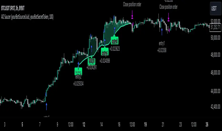
MultiLayer Awesome Oscillator Saucer Strategy [Skyrexio]Overview
MultiLayer Awesome Oscillator Saucer Strategy leverages the combination of Awesome Oscillator (AO), Williams Alligator, Williams Fractals and Exponential Moving Average (EMA) to obtain the high probability long setups. Moreover, strategy uses multi trades system, adding funds to long position if it considered that current trend has likely became stronger. Awesome Oscillator is used for creating signals, while Alligator and Fractal are used in conjunction as an approximation of short-term trend to filter them. At the same time EMA (default EMA's period = 100) is used as high probability long-term trend filter to open long trades only if it considers current price action as an uptrend. More information in "Methodology" and "Justification of Methodology" paragraphs. The strategy opens only long trades.
Unique Features
No fixed stop-loss and take profit: Instead of fixed stop-loss level strategy utilizes technical condition obtained by Fractals and Alligator to identify when current uptrend is likely to be over (more information in "Methodology" and "Justification of Methodology" paragraphs)
Configurable Trading Periods: Users can tailor the strategy to specific market windows, adapting to different market conditions.
Multilayer trades opening system: strategy uses only 10% of capital in every trade and open up to 5 trades at the same time if script consider current trend as strong one.
Short and long term trend trade filters: strategy uses EMA as high probability long-term trend filter and Alligator and Fractal combination as a short-term one.
Methodology
The strategy opens long trade when the following price met the conditions:
1. Price closed above EMA (by default, period = 100). Crossover is not obligatory.
2. Combination of Alligator and Williams Fractals shall consider current trend as an upward (all details in "Justification of Methodology" paragraph)
3. Awesome Oscillator shall create the "Saucer" long signal (all details in "Justification of Methodology" paragraph). Buy stop order is placed one tick above the candle's high of last created "Saucer signal".
4. If price reaches the order price, long position is opened with 10% of capital.
5. If currently we have opened position and price creates and hit the order price of another one "Saucer" signal another one long position will be added to the previous with another one 10% of capital. Strategy allows to open up to 5 long trades simultaneously.
6. If combination of Alligator and Williams Fractals shall consider current trend has been changed from up to downtrend, all long trades will be closed, no matter how many trades has been opened.
Script also has additional visuals. If second long trade has been opened simultaneously the Alligator's teeth line is plotted with the green color. Also for every trade in a row from 2 to 5 the label "Buy More" is also plotted just below the teeth line. With every next simultaneously opened trade the green color of the space between teeth and price became less transparent.
Strategy settings
In the inputs window user can setup strategy setting: EMA Length (by default = 100, period of EMA, used for long-term trend filtering EMA calculation). User can choose the optimal parameters during backtesting on certain price chart.
Justification of Methodology
Let's go through all concepts used in this strategy to understand how they works together. Let's start from the easies one, the EMA. Let's briefly explain what is EMA. The Exponential Moving Average (EMA) is a type of moving average that gives more weight to recent prices, making it more responsive to current price changes compared to the Simple Moving Average (SMA). It is commonly used in technical analysis to identify trends and generate buy or sell signals. It can be calculated with the following steps:
1.Calculate the Smoothing Multiplier:
Multiplier = 2 / (n + 1), Where n is the number of periods.
2. EMA Calculation
EMA = (Current Price) × Multiplier + (Previous EMA) × (1 − Multiplier)
In this strategy uses EMA an initial long term trend filter. It allows to open long trades only if price close above EMA (by default 50 period). It increases the probability of taking long trades only in the direction of the trend.
Let's go to the next, short-term trend filter which consists of Alligator and Fractals. Let's briefly explain what do these indicators means. The Williams Alligator, developed by Bill Williams, is a technical indicator designed to spot trends and potential market reversals. It uses three smoothed moving averages, referred to as the jaw, teeth, and lips:
Jaw (Blue Line): The slowest of the three, based on a 13-period smoothed moving average shifted 8 bars ahead.
Teeth (Red Line): The medium-speed line, derived from an 8-period smoothed moving average shifted 5 bars forward.
Lips (Green Line): The fastest line, calculated using a 5-period smoothed moving average shifted 3 bars forward.
When these lines diverge and are properly aligned, the "alligator" is considered "awake," signaling a strong trend. Conversely, when the lines overlap or intertwine, the "alligator" is "asleep," indicating a range-bound or sideways market. This indicator assists traders in identifying when to act on or avoid trades.
The Williams Fractals, another tool introduced by Bill Williams, are used to pinpoint potential reversal points on a price chart. A fractal forms when there are at least five consecutive bars, with the middle bar displaying the highest high (for an up fractal) or the lowest low (for a down fractal), relative to the two bars on either side.
Key Points:
Up Fractal: Occurs when the middle bar has a higher high than the two preceding and two following bars, suggesting a potential downward reversal.
Down Fractal: Happens when the middle bar shows a lower low than the surrounding two bars, hinting at a possible upward reversal.
Traders often combine fractals with other indicators to confirm trends or reversals, improving the accuracy of trading decisions.
How we use their combination in this strategy? Let’s consider an uptrend example. A breakout above an up fractal can be interpreted as a bullish signal, indicating a high likelihood that an uptrend is beginning. Here's the reasoning: an up fractal represents a potential shift in market behavior. When the fractal forms, it reflects a pullback caused by traders selling, creating a temporary high. However, if the price manages to return to that fractal’s high and break through it, it suggests the market has "changed its mind" and a bullish trend is likely emerging.
The moment of the breakout marks the potential transition to an uptrend. It’s crucial to note that this breakout must occur above the Alligator's teeth line. If it happens below, the breakout isn’t valid, and the downtrend may still persist. The same logic applies inversely for down fractals in a downtrend scenario.
So, if last up fractal breakout was higher, than Alligator's teeth and it happened after last down fractal breakdown below teeth, algorithm considered current trend as an uptrend. During this uptrend long trades can be opened if signal was flashed. If during the uptrend price breaks down the down fractal below teeth line, strategy considered that uptrend is finished with the high probability and strategy closes all current long trades. This combination is used as a short term trend filter increasing the probability of opening profitable long trades in addition to EMA filter, described above.
Now let's talk about Awesome Oscillator's "Sauser" signals. Briefly explain what is the Awesome Oscillator. The Awesome Oscillator (AO), created by Bill Williams, is a momentum-based indicator that evaluates market momentum by comparing recent price activity to a broader historical context. It assists traders in identifying potential trend reversals and gauging trend strength.
AO = SMA5(Median Price) − SMA34(Median Price)
where:
Median Price = (High + Low) / 2
SMA5 = 5-period Simple Moving Average of the Median Price
SMA 34 = 34-period Simple Moving Average of the Median Price
Now we know what is AO, but what is the "Saucer" signal? This concept was introduced by Bill Williams, let's briefly explain it and how it's used by this strategy. Initially, this type of signal is a combination of the following AO bars: we need 3 bars in a row, the first one shall be higher than the second, the third bar also shall be higher, than second. All three bars shall be above the zero line of AO. The price bar, which corresponds to third "saucer's" bar is our signal bar. Strategy places buy stop order one tick above the price bar which corresponds to signal bar.
After that we can have the following scenarios.
Price hit the order on the next candle in this case strategy opened long with this price.
Price doesn't hit the order price, the next candle set lower low. If current AO bar is increasing buy stop order changes by the script to the high of this new bar plus one tick. This procedure repeats until price finally hit buy order or current AO bar become decreasing. In the second case buy order cancelled and strategy wait for the next "Saucer" signal.
If long trades has been opened strategy use all the next signals until number of trades doesn't exceed 5. All trades are closed when the trend changes to downtrend according to combination of Alligator and Fractals described above.
Why we use "Saucer" signals? If AO above the zero line there is a high probability that price now is in uptrend if we take into account our two trend filters. When we see the decreasing bars on AO and it's above zero it's likely can be considered as a pullback on the uptrend. When we see the stop of AO decreasing and the first increasing bar has been printed there is a high probability that this local pull back is finished and strategy open long trade in the likely direction of a main trend.
Why strategy use only 10% per signal? Sometimes we can see the false signals which appears on sideways. Not risking that much script use only 10% per signal. If the first long trade has been open and price continue going up and our trend approximation by Alligator and Fractals is uptrend, strategy add another one 10% of capital to every next saucer signal while number of active trades no more than 5. This capital allocation allows to take part in long trades when current uptrend is likely to be strong and use only 10% of capital when there is a high probability of sideways.
Backtest Results
Operating window: Date range of backtests is 2023.01.01 - 2024.11.25. It is chosen to let the strategy to close all opened positions.
Commission and Slippage: Includes a standard Binance commission of 0.1% and accounts for possible slippage over 5 ticks.
Initial capital: 10000 USDT
Percent of capital used in every trade: 10%
Maximum Single Position Loss: -5.10%
Maximum Single Profit: +22.80%
Net Profit: +2838.58 USDT (+28.39%)
Total Trades: 107 (42.99% win rate)
Profit Factor: 3.364
Maximum Accumulated Loss: 373.43 USDT (-2.98%)
Average Profit per Trade: 26.53 USDT (+2.40%)
Average Trade Duration: 78 hours
These results are obtained with realistic parameters representing trading conditions observed at major exchanges such as Binance and with realistic trading portfolio usage parameters.
How to Use
Add the script to favorites for easy access.
Apply to the desired timeframe and chart (optimal performance observed on 3h BTC/USDT).
Configure settings using the dropdown choice list in the built-in menu.
Set up alerts to automate strategy positions through web hook with the text: {{strategy.order.alert_message}}
Disclaimer:
Educational and informational tool reflecting Skyrex commitment to informed trading. Past performance does not guarantee future results. Test strategies in a simulated environment before live implementation
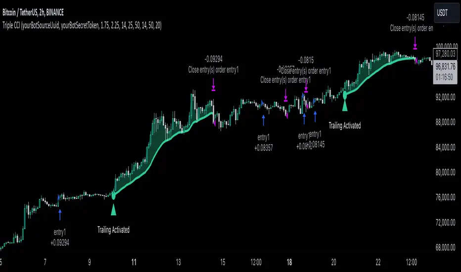
Triple CCI Strategy MFI Confirmed [Skyrexio]Overview
Triple CCI Strategy MFI Confirmed leverages 3 different periods Commodity Channel Index (CCI) indicator in conjunction Money Flow Index (MFI) and Exponential Moving Average (EMA) to obtain the high probability setups. Fast period CCI is used for having the high probability to enter in the direction of short term trend, middle and slow period CCI are used for confirmation, if market now likely in the mid and long-term uptrend. MFI is used to confirm trade with the money inflow/outflow with the high probability. EMA is used as an additional trend filter. Moreover, strategy uses exponential moving average (EMA) to trail the price when it reaches the specific level. More information in "Methodology" and "Justification of Methodology" paragraphs. The strategy opens only long trades.
Unique Features
Dynamic stop-loss system: Instead of fixed stop-loss level strategy utilizes average true range (ATR) multiplied by user given number subtracted from the position entry price as a dynamic stop loss level.
Configurable Trading Periods: Users can tailor the strategy to specific market windows, adapting to different market conditions.
Four layers trade filtering system: Strategy utilizes two different period CCI indicators, MFI and EMA indicators to confirm the signals produced by fast period CCI.
Trailing take profit level: After reaching the trailing profit activation level scrip activate the trailing of long trade using EMA. More information in methodology.
Methodology
The strategy opens long trade when the following price met the conditions:
Fast period CCI shall crossover the zero-line.
Slow and Middle period CCI shall be above zero-lines.
Price shall close above the EMA. Crossover is not obligatory
MFI shall be above 50
When long trade is executed, strategy set the stop-loss level at the price ATR multiplied by user-given value below the entry price. This level is recalculated on every next candle close, adjusting to the current market volatility.
At the same time strategy set up the trailing stop validation level. When the price crosses the level equals entry price plus ATR multiplied by user-given value script starts to trail the price with EMA. If price closes below EMA long trade is closed. When the trailing starts, script prints the label “Trailing Activated”.
Strategy settings
In the inputs window user can setup the following strategy settings:
ATR Stop Loss (by default = 1.75)
ATR Trailing Profit Activation Level (by default = 2.25)
CCI Fast Length (by default = 14, used for calculation short term period CCI)
CCI Middle Length (by default = 25, used for calculation short term period CCI)
CCI Slow Length (by default = 50, used for calculation long term period CCI)
MFI Length (by default = 14, used for calculation MFI
EMA Length (by default = 50, period of EMA, used for trend filtering EMA calculation)
Trailing EMA Length (by default = 20)
User can choose the optimal parameters during backtesting on certain price chart.
Justification of Methodology
Before understanding why this particular combination of indicator has been chosen let's briefly explain what is CCI, MFI and EMA.
The Commodity Channel Index (CCI) is a momentum-based technical indicator that measures the deviation of a security's price from its average price over a specific period. It helps traders identify overbought or oversold conditions and potential trend reversals.
The CCI formula is:
CCI = (Typical Price − SMA) / (0.015 × Mean Deviation)
Typical Price (TP): This is calculated as the average of the high, low, and closing prices for the period.
Simple Moving Average (SMA): This is the average of the Typical Prices over a specific number of periods.
Mean Deviation: This is the average of the absolute differences between the Typical Price and the SMA.
The result is a value that typically fluctuates between +100 and -100, though it is not bounded and can go higher or lower depending on the price movement.
The Money Flow Index (MFI) is a technical indicator that measures the strength of money flowing into and out of a security. It combines price and volume data to assess buying and selling pressure and is often used to identify overbought or oversold conditions. The formula for MFI involves several steps:
1. Calculate the Typical Price (TP):
TP = (high + low + close) / 3
2. Calculate the Raw Money Flow (RMF):
Raw Money Flow = TP × Volume
3. Determine Positive and Negative Money Flow:
If the current TP is greater than the previous TP, it's Positive Money Flow.
If the current TP is less than the previous TP, it's Negative Money Flow.
4. Calculate the Money Flow Ratio (MFR):
Money Flow Ratio = Sum of Positive Money Flow (over n periods) / Sum of Negative Money Flow (over n periods)
5. Calculate the Money Flow Index (MFI):
MFI = 100 − (100 / (1 + Money Flow Ratio))
MFI above 80 can be considered as overbought, below 20 - oversold.
The Exponential Moving Average (EMA) is a type of moving average that places greater weight and significance on the most recent data points. It is widely used in technical analysis to smooth price data and identify trends more quickly than the Simple Moving Average (SMA).
Formula:
1. Calculate the multiplier
Multiplier = 2 / (n + 1) , Where n is the number of periods.
2. EMA Calculation
EMA = (Current Price) × Multiplier + (Previous EMA) × (1 − Multiplier)
This strategy leverages Fast period CCI, which shall break the zero line to the upside to say that probability of short term trend change to the upside increased. This zero line crossover shall be confirmed by the Middle and Slow periods CCI Indicators. At the moment of breakout these two CCIs shall be above 0, indicating that there is a high probability that price is in middle and long term uptrend. This approach increases chances to have a long trade setup in the direction of mid-term and long-term trends when the short-term trend starts to reverse to the upside.
Additionally strategy uses MFI to have a greater probability that fast CCI breakout is confirmed by this indicator. We consider the values of MFI above 50 as a higher probability that trend change from downtrend to the uptrend is real. Script opens long trades only if MFI is above 50. As you already know from the MFI description, it incorporates volume in its calculation, therefore we have another one confirmation factor.
Finally, strategy uses EMA an additional trend filter. It allows to open long trades only if price close above EMA (by default 50 period). It increases the probability of taking long trades only in the direction of the trend.
ATR is used to adjust the strategy risk management to the current market volatility. If volatility is low, we don’t need the large stop loss to understand the there is a high probability that we made a mistake opening the trade. User can setup the settings ATR Stop Loss and ATR Trailing Profit Activation Level to realize his own risk to reward preferences, but the unique feature of a strategy is that after reaching trailing profit activation level strategy is trying to follow the trend until it is likely to be finished instead of using fixed risk management settings. It allows sometimes to be involved in the large movements. It’s also important to make a note, that script uses another one EMA (by default = 20 period) as a trailing profit level.
Backtest Results
Operating window: Date range of backtests is 2022.04.01 - 2024.11.25. It is chosen to let the strategy to close all opened positions.
Commission and Slippage: Includes a standard Binance commission of 0.1% and accounts for possible slippage over 5 ticks.
Initial capital: 10000 USDT
Percent of capital used in every trade: 50%
Maximum Single Position Loss: -4.13%
Maximum Single Profit: +19.66%
Net Profit: +5421.21 USDT (+54.21%)
Total Trades: 108 (44.44% win rate)
Profit Factor: 2.006
Maximum Accumulated Loss: 777.40 USDT (-7.77%)
Average Profit per Trade: 50.20 USDT (+0.85%)
Average Trade Duration: 44 hours
These results are obtained with realistic parameters representing trading conditions observed at major exchanges such as Binance and with realistic trading portfolio usage parameters.
How to Use
Add the script to favorites for easy access.
Apply to the desired timeframe and chart (optimal performance observed on 2h BTC/USDT).
Configure settings using the dropdown choice list in the built-in menu.
Set up alerts to automate strategy positions through web hook with the text: {{strategy.order.alert_message}}
Disclaimer:
Educational and informational tool reflecting Skyrex commitment to informed trading. Past performance does not guarantee future results. Test strategies in a simulated environment before live implementation
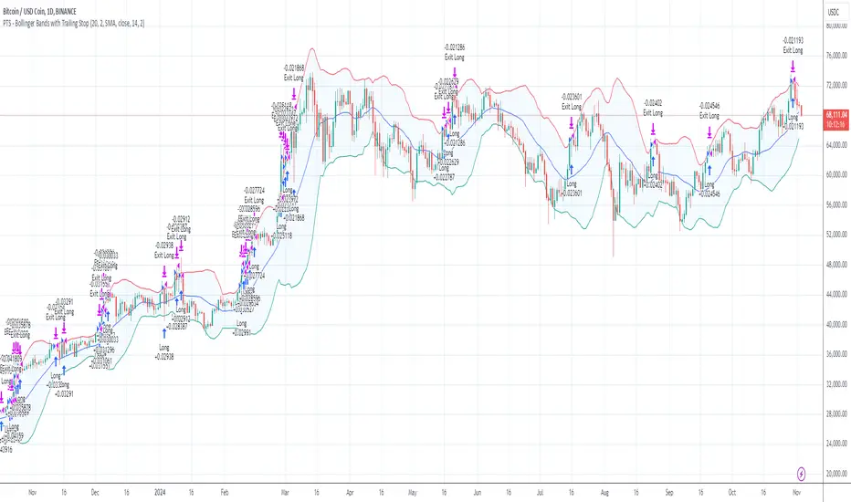
PTS - Bollinger Bands with Trailing StopPTS - Bollinger Bands with Trailing Stop Strategy
Overview
The "PTS - Bollinger Bands with Trailing Stop" strategy is designed to capitalize on strong bullish market movements by combining the Bollinger Bands indicator with a dynamic trailing stop based on the Average True Range (ATR). This strategy aims to enter long positions during upward breakouts and protect profits through an adaptive exit mechanism.
Key Features
1. Bollinger Bands Indicator
Basis Moving Average Type: Choose from SMA, EMA, SMMA, WMA, or VWMA for the Bollinger Bands' basis line. Length: Adjustable period for calculating the moving average and standard deviation (default is 20). Standard Deviation Multiplier (StdDev): Determines the width of the bands (default is 2.0). Source: Select the price data used for calculations (default is the closing price).
2. Entry Conditions
The strategy enters a long position when the closing price crosses above the upper Bollinger Band , indicating strong upward momentum.
3. Exit Conditions
Trailing Stop Loss: Implemented using ATR to adjust dynamically with market volatility. ATR Length: Period for calculating ATR (default is 14). ATR Multiplier for Trailing Stop: Determines how closely the trailing stop follows the price (default is 2.0). Close Below Lower Bollinger Band: The strategy exits the long position if the closing price crosses below the lower Bollinger Band .
4. Risk Management
Commission and Slippage: Commission is set at 0.1%; slippage is set to 3. Position Sizing: Uses 100% of equity per trade (adjustable).
5. Date Range Filter
Specify the time period during which the strategy is active. Start Date: January 1, 2018. End Date: December 31, 2069.
Customizable Inputs
BB Length: Adjust the period for Bollinger Bands calculation. BB StdDev: Modify the standard deviation multiplier. Basis MA Type: Select the moving average type. Source: Choose the price data source. Offset: Shift the Bollinger Bands on the chart. ATR Length: Set the period for ATR calculation. ATR Multiplier for Trailing Stop: Adjust the trailing stop sensitivity.
Thought for 1m 7s
Description for the "PTS - Bollinger Bands with Trailing Stop" Strategy
PTS - Bollinger Bands with Trailing Stop Strategy
Overview
The "PTS - Bollinger Bands with Trailing Stop" strategy is designed to capitalize on strong bullish market movements by combining the Bollinger Bands indicator with a dynamic trailing stop based on the Average True Range (ATR). This strategy aims to enter long positions during upward breakouts and protect profits through an adaptive exit mechanism.
Key Features
1. Bollinger Bands Indicator
Basis Moving Average Type: Choose from SMA, EMA, SMMA, WMA, or VWMA for the Bollinger Bands' basis line. Length: Adjustable period for calculating the moving average and standard deviation (default is 20). Standard Deviation Multiplier (StdDev): Determines the width of the bands (default is 2.0). Source: Select the price data used for calculations (default is the closing price).
2. Entry Conditions
The strategy enters a long position when the closing price crosses above the upper Bollinger Band , indicating strong upward momentum.
3. Exit Conditions
Trailing Stop Loss: Implemented using ATR to adjust dynamically with market volatility. ATR Length: Period for calculating ATR (default is 14). ATR Multiplier for Trailing Stop: Determines how closely the trailing stop follows the price (default is 2.0). Close Below Lower Bollinger Band: The strategy exits the long position if the closing price crosses below the lower Bollinger Band .
4. Risk Management
Commission and Slippage: Commission is set at 0.1%; slippage is set to 3. Position Sizing: Uses 100% of equity per trade (adjustable).
5. Date Range Filter
Specify the time period during which the strategy is active. Start Date: January 1, 2018. End Date: December 31, 2069.
Customizable Inputs
BB Length: Adjust the period for Bollinger Bands calculation. BB StdDev: Modify the standard deviation multiplier. Basis MA Type: Select the moving average type. Source: Choose the price data source. Offset: Shift the Bollinger Bands on the chart. ATR Length: Set the period for ATR calculation. ATR Multiplier for Trailing Stop: Adjust the trailing stop sensitivity.
How the Strategy Works
1. Initialization
Calculates Bollinger Bands and ATR based on selected parameters.
2. Entry Logic
Opens a long position when the closing price exceeds the upper Bollinger Band.
3. Exit Logic
Uses a trailing stop loss based on ATR. Exits if the closing price drops below the lower Bollinger Band.
4. Date Filtering
Executes trades only within the specified date range.
Advantages
Adaptive Risk Management: Trailing stop adjusts to market volatility. Simplicity: Clear entry and exit signals. Customizable Parameters: Tailor the strategy to different assets or conditions.
Considerations
Aggressive Position Sizing: Using 100% equity per trade is high-risk. Market Conditions: Best in trending markets; may produce false signals in sideways markets. Backtesting: Always test on historical data before live trading.
Disclaimer
This strategy is intended for educational and informational purposes only. Trading involves significant risk, and past performance is not indicative of future results. Assess your financial situation and consult a financial advisor if necessary.
Usage Instructions
1. Apply the Strategy: Add it to your TradingView chart. 2. Configure Inputs: Adjust parameters to suit your style and asset. 3. Analyze Backtest Results: Use the Strategy Tester. 4. Optimize Parameters: Experiment with input values. 5. Risk Management: Evaluate position sizing and incorporate risk controls.
Final Notes
The "PTS - Bollinger Bands with Trailing Stop" strategy provides a framework to leverage momentum breakouts while managing risk through adaptive trailing stops. Customize and test thoroughly to align with your trading objectives.
[Defaust] Fractals Fractals Indicator
Overview
The Fractals Indicator is a technical analysis tool designed to help traders identify potential reversal points in the market by detecting fractal patterns. This indicator is a fork of the original fractals indicator, with adjustments made to the plotting for enhanced visual clarity and usability.
What Are Fractals?
In trading, a fractal is a pattern consisting of five consecutive bars (candlesticks) that meet specific conditions:
Up Fractal (Potential Sell Signal): Occurs when a high point is surrounded by two lower highs on each side.
Down Fractal (Potential Buy Signal): Occurs when a low point is surrounded by two higher lows on each side.
Fractals help traders identify potential tops and bottoms in the market, signaling possible entry or exit points.
Features of the Indicator
Customizable Periods (n): Allows you to define the number of periods to consider when detecting fractals, offering flexibility to adapt to different trading strategies and timeframes.
Enhanced Plotting Adjustments: This fork introduces adjustments to the plotting of fractal signals for better visual representation on the chart.
Visual Signals: Plots up and down triangles on the chart to signify down fractals (potential bullish signals) and up fractals (potential bearish signals), respectively.
Overlay on Chart: The fractal signals are overlaid directly on the price chart for immediate visualization.
Adjustable Precision: You can set the precision of the plotted values according to your needs.
Pine Script Code Explanation
Below is the Pine Script code for the Fractals Indicator:
//@version=5 indicator(" Fractals", shorttitle=" Fractals", format=format.price, precision=0, overlay=true)
// User input for the number of periods to consider for fractal detection n = input.int(title="Periods", defval=2, minval=2)
// Initialize flags for up fractal detection bool upflagDownFrontier = true bool upflagUpFrontier0 = true bool upflagUpFrontier1 = true bool upflagUpFrontier2 = true bool upflagUpFrontier3 = true bool upflagUpFrontier4 = true
// Loop through previous and future bars to check conditions for up fractals for i = 1 to n // Check if the highs of previous bars are less than the current bar's high upflagDownFrontier := upflagDownFrontier and (high < high ) // Check various conditions for future bars upflagUpFrontier0 := upflagUpFrontier0 and (high < high ) upflagUpFrontier1 := upflagUpFrontier1 and (high <= high and high < high ) upflagUpFrontier2 := upflagUpFrontier2 and (high <= high and high <= high and high < high ) upflagUpFrontier3 := upflagUpFrontier3 and (high <= high and high <= high and high <= high and high < high ) upflagUpFrontier4 := upflagUpFrontier4 and (high <= high and high <= high and high <= high and high <= high and high < high )
// Combine the flags to determine if an up fractal exists flagUpFrontier = upflagUpFrontier0 or upflagUpFrontier1 or upflagUpFrontier2 or upflagUpFrontier3 or upflagUpFrontier4 upFractal = (upflagDownFrontier and flagUpFrontier)
// Initialize flags for down fractal detection bool downflagDownFrontier = true bool downflagUpFrontier0 = true bool downflagUpFrontier1 = true bool downflagUpFrontier2 = true bool downflagUpFrontier3 = true bool downflagUpFrontier4 = true
// Loop through previous and future bars to check conditions for down fractals for i = 1 to n // Check if the lows of previous bars are greater than the current bar's low downflagDownFrontier := downflagDownFrontier and (low > low ) // Check various conditions for future bars downflagUpFrontier0 := downflagUpFrontier0 and (low > low ) downflagUpFrontier1 := downflagUpFrontier1 and (low >= low and low > low ) downflagUpFrontier2 := downflagUpFrontier2 and (low >= low and low >= low and low > low ) downflagUpFrontier3 := downflagUpFrontier3 and (low >= low and low >= low and low >= low and low > low ) downflagUpFrontier4 := downflagUpFrontier4 and (low >= low and low >= low and low >= low and low >= low and low > low )
// Combine the flags to determine if a down fractal exists flagDownFrontier = downflagUpFrontier0 or downflagUpFrontier1 or downflagUpFrontier2 or downflagUpFrontier3 or downflagUpFrontier4 downFractal = (downflagDownFrontier and flagDownFrontier)
// Plot the fractal symbols on the chart with adjusted plotting plotshape(downFractal, style=shape.triangleup, location=location.belowbar, offset=-n, color=color.gray, size=size.auto) plotshape(upFractal, style=shape.triangledown, location=location.abovebar, offset=-n, color=color.gray, size=size.auto)
Explanation:
Input Parameter (n): Sets the number of periods for fractal detection. The default value is 2, and it must be at least 2 to ensure valid fractal patterns.
Flag Initialization: Boolean variables are used to store intermediate conditions during fractal detection.
Loops: Iterate through the specified number of periods to evaluate the conditions for fractal formation.
Conditions:
Up Fractals: Checks if the current high is greater than previous highs and if future highs are lower or equal to the current high.
Down Fractals: Checks if the current low is lower than previous lows and if future lows are higher or equal to the current low.
Flag Combination: Logical and and or operations are used to combine the flags and determine if a fractal exists.
Adjusted Plotting:
The plotting of fractal symbols has been adjusted for better alignment and visual clarity.
The offset parameter is set to -n to align the plotted symbols with the correct bars.
The color and size have been fine-tuned for better visibility.
How to Use the Indicator
Adding the Indicator to Your Chart
Open TradingView:
Go to TradingView.
Access the Chart:
Click on "Chart" to open the main charting interface.
Add the Indicator:
Click on the "Indicators" button at the top.
Search for " Fractals".
Select the indicator from the list to add it to your chart.
Configuring the Indicator
Periods (n):
Default value is 2.
Adjust this parameter based on your preferred timeframe and sensitivity.
A higher value of n considers more bars for fractal detection, potentially reducing the number of signals but increasing their significance.
Interpreting the Signals
– Up Fractal (Downward Triangle): Indicates a potential price reversal to the downside. May be used as a signal to consider exiting long positions or tightening stop-loss orders.
– Down Fractal (Upward Triangle): Indicates a potential price reversal to the upside. May be used as a signal to consider entering long positions or setting stop-loss orders for short positions.
Trading Strategy Suggestions
Up Fractal Detection:
The high of the current bar (n) is higher than the highs of the previous two bars (n - 1, n - 2).
The highs of the next bars meet certain conditions to confirm the fractal pattern.
An up fractal symbol (downward triangle) is plotted above the bar at position n - n (due to the offset).
Down Fractal Detection:
The low of the current bar (n) is lower than the lows of the previous two bars (n - 1, n - 2).
The lows of the next bars meet certain conditions to confirm the fractal pattern.
A down fractal symbol (upward triangle) is plotted below the bar at position n - n.
Benefits of Using the Fractals Indicator
Early Signals: Helps in identifying potential reversal points in price movements.
Customizable Sensitivity: Adjusting the n parameter allows you to fine-tune the indicator based on different market conditions.
Enhanced Visuals: Adjustments to plotting improve the clarity and readability of fractal signals on the chart.
Limitations and Considerations
Lagging Indicator: Fractals require future bars to confirm the pattern, which may introduce a delay in the signals.
False Signals: In volatile or ranging markets, fractals may produce false signals. It's advisable to use them in conjunction with other analysis tools.
Not a Standalone Tool: Fractals should be part of a broader trading strategy that includes other indicators and fundamental analysis.
Best Practices for Using This Indicator
Combine with Other Indicators: Use in combination with trend indicators, oscillators, or volume analysis to confirm signals.
Backtesting: Before applying the indicator in live trading, backtest it on historical data to understand its performance.
Adjust Periods Accordingly: Experiment with different values of n to find the optimal setting for the specific asset and timeframe you are trading.
Disclaimer
The Fractals Indicator is intended for educational and informational purposes only. Trading involves significant risk, and you should be aware of the risks involved before proceeding. Past performance is not indicative of future results. Always conduct your own analysis and consult with a professional financial advisor before making any investment decisions.
Credits
This indicator is a fork of the original fractals indicator, with adjustments made to the plotting for improved visual representation. It is based on standard fractal patterns commonly used in technical analysis and has been developed to provide traders with an effective tool for detecting potential reversal points in the market.
Uptrick: RSI Histogram
1. **Introduction to the RSI and Moving Averages**
2. **Detailed Breakdown of the Uptrick: RSI Histogram**
3. **Calculation and Formula**
4. **Visual Representation**
5. **Customization and User Settings**
6. **Trading Strategies and Applications**
7. **Risk Management**
8. **Case Studies and Examples**
9. **Comparison with Other Indicators**
10. **Advanced Usage and Tips**
---
## 1. Introduction to the RSI and Moving Averages
### **1.1 Relative Strength Index (RSI)**
The Relative Strength Index (RSI) is a momentum oscillator developed by J. Welles Wilder and introduced in his 1978 book "New Concepts in Technical Trading Systems." It is widely used in technical analysis to measure the speed and change of price movements.
**Purpose of RSI:**
- **Identify Overbought/Oversold Conditions:** RSI values range from 0 to 100. Traditionally, values above 70 are considered overbought, while values below 30 are considered oversold. These thresholds help traders identify potential reversal points in the market.
- **Trend Strength Measurement:** RSI also indicates the strength of a trend. High RSI values suggest strong bullish momentum, while low values indicate bearish momentum.
**Calculation of RSI:**
1. **Calculate the Average Gain and Loss:** Over a specified period (e.g., 14 days), calculate the average gain and loss.
2. **Compute the Relative Strength (RS):** RS is the ratio of average gain to average loss.
3. **RSI Formula:** RSI = 100 - (100 / (1 + RS))
### **1.2 Moving Averages (MA)**
Moving Averages are used to smooth out price data and identify trends by filtering out short-term fluctuations. Two common types are:
**Simple Moving Average (SMA):** The average of prices over a specified number of periods.
**Exponential Moving Average (EMA):** A type of moving average that gives more weight to recent prices, making it more responsive to recent price changes.
**Smoothed Moving Average (SMA):** Used to reduce the impact of volatility and provide a clearer view of the underlying trend. The RMA, or Running Moving Average, used in the USH script is similar to an EMA but based on the average of RSI values.
## 2. Detailed Breakdown of the Uptrick: RSI Histogram
### **2.1 Indicator Overview**
The Uptrick: RSI Histogram (USH) is a technical analysis tool that combines the RSI with a moving average to create a histogram that reflects momentum and trend strength.
**Key Components:**
- **RSI Calculation:** Determines the relative strength of price movements.
- **Moving Average Application:** Smooths the RSI values to provide a clearer trend indication.
- **Histogram Plotting:** Visualizes the deviation of the smoothed RSI from a neutral level.
### **2.2 Indicator Purpose**
The primary purpose of the USH is to provide a clear visual representation of the market's momentum and trend strength. It helps traders identify:
- **Bullish and Bearish Trends:** By showing how far the smoothed RSI is from the neutral 50 level.
- **Potential Reversal Points:** By highlighting changes in momentum.
### **2.3 Indicator Design**
**RSI Moving Average (RSI MA):** The RSI MA is a smoothed version of the RSI, calculated using a running moving average. This smooths out short-term fluctuations and provides a clearer indication of the underlying trend.
**Histogram Calculation:**
- **Neutral Level:** The histogram is plotted relative to the neutral level of 50. This level represents a balanced market where neither bulls nor bears have dominance.
- **Histogram Values:** The histogram bars show the difference between the RSI MA and the neutral level. Positive values indicate bullish momentum, while negative values indicate bearish momentum.
## 3. Calculation and Formula
### **3.1 RSI Calculation**
The RSI calculation involves:
1. **Average Gain and Loss:** Calculated over the specified length (e.g., 14 periods).
2. **Relative Strength (RS):** RS = Average Gain / Average Loss.
3. **RSI Formula:** RSI = 100 - (100 / (1 + RS)).
### **3.2 Moving Average Calculation**
For the USH indicator, the RSI is smoothed using a running moving average (RMA). The RMA formula is similar to that of the EMA but is based on averaging RSI values over the specified length.
### **3.3 Histogram Calculation**
The histogram value is calculated as:
- **Histogram Value = RSI MA - 50**
**Plotting the Histogram:**
- **Positive Histogram Values:** Indicate that the RSI MA is above the neutral level, suggesting bullish momentum.
- **Negative Histogram Values:** Indicate that the RSI MA is below the neutral level, suggesting bearish momentum.
## 4. Visual Representation
### **4.1 Histogram Bars**
The histogram is plotted as bars on the chart:
- **Bullish Bars:** Colored green when the RSI MA is above 50.
- **Bearish Bars:** Colored red when the RSI MA is below 50.
### **4.2 Customization Options**
Traders can customize:
- **RSI Length:** Adjust the length of the RSI calculation to match their trading style.
- **Bull and Bear Colors:** Choose colors for histogram bars to enhance visual clarity.
### **4.3 Interpretation**
**Bullish Signal:** A histogram bar that moves from red to green indicates a potential shift to a bullish trend.
**Bearish Signal:** A histogram bar that moves from green to red indicates a potential shift to a bearish trend.
## 5. Customization and User Settings
### **5.1 Adjusting RSI Length**
The length parameter determines the number of periods over which the RSI is calculated and smoothed. Shorter lengths make the RSI more sensitive to price changes, while longer lengths provide a smoother view of trends.
### **5.2 Color Settings**
Traders can adjust:
- **Bull Color:** Color of histogram bars indicating bullish momentum.
- **Bear Color:** Color of histogram bars indicating bearish momentum.
**Customization Benefits:**
- **Visual Clarity:** Traders can choose colors that stand out against their chart’s background.
- **Personal Preference:** Adjust settings to match individual trading styles and preferences.
## 6. Trading Strategies and Applications
### **6.1 Trend Following**
**Identifying Entry Points:**
- **Bullish Entry:** When the histogram changes from red to green, it signals a potential entry point for long positions.
- **Bearish Entry:** When the histogram changes from green to red, it signals a potential entry point for short positions.
**Trend Confirmation:** The histogram helps confirm the strength of a trend. Strong, consistent green bars indicate robust bullish momentum, while strong, consistent red bars indicate robust bearish momentum.
### **6.2 Swing Trading**
**Momentum Analysis:**
- **Entry Signals:** Look for significant shifts in the histogram to time entries. A shift from bearish to bullish (red to green) indicates potential for upward movement.
- **Exit Signals:** A shift from bullish to bearish (green to red) suggests a potential weakening of the trend, signaling an exit or reversal point.
### **6.3 Range Trading**
**Market Conditions:**
- **Consolidation:** The histogram close to zero suggests a range-bound market. Traders can use this information to identify support and resistance levels.
- **Breakout Potential:** A significant move away from the neutral level may indicate a potential breakout from the range.
### **6.4 Risk Management**
**Stop-Loss Placement:**
- **Bullish Positions:** Place stop-loss orders below recent support levels when the histogram is green.
- **Bearish Positions:** Place stop-loss orders above recent resistance levels when the histogram is red.
**Position Sizing:** Adjust position sizes based on the strength of the histogram signals. Strong trends (indicated by larger histogram bars) may warrant larger positions, while weaker signals suggest smaller positions.
## 7. Risk Management
### **7.1 Importance of Risk Management**
Effective risk management is crucial for long-term trading success. It involves protecting capital, managing losses, and optimizing trade setups.
### **7.2 Using USH for Risk Management**
**Stop-Loss and Take-Profit Levels:**
- **Stop-Loss Orders:** Use the histogram to set stop-loss levels based on trend strength. For instance, place stops below support levels in bullish trends and above resistance levels in bearish trends.
- **Take-Profit Targets:** Adjust take-profit levels based on histogram changes. For example, lock in profits as the histogram starts to shift from green to red.
**Position Sizing:**
- **Trend Strength:** Scale position sizes based on the strength of histogram signals. Larger histogram bars indicate stronger trends, which may justify larger positions.
- **Volatility:** Consider market volatility and adjust position sizes to mitigate risk.
## 8. Case Studies and Examples
### **8.1 Example 1: Bullish Trend**
**Scenario:** A trader notices a transition from red to green histogram bars.
**Analysis:**
- **Entry Point:** The transition indicates a potential bullish trend. The trader decides to enter a long position.
- **Stop-Loss:** Set stop-loss below recent support levels.
- **Take-Profit:** Consider taking profits as the histogram moves back towards zero or turns red.
**Outcome:** The bullish trend continues, and the histogram remains green, providing a profitable trade setup.
### **8.2 Example 2: Bearish Trend**
**Scenario:** A trader observes a transition from green to red histogram bars.
**Analysis:**
- **Entry Point:** The transition suggests a potential
bearish trend. The trader decides to enter a short position.
- **Stop-Loss:** Set stop-loss above recent resistance levels.
- **Take-Profit:** Consider taking profits as the histogram approaches zero or shifts to green.
**Outcome:** The bearish trend continues, and the histogram remains red, resulting in a successful trade.
## 9. Comparison with Other Indicators
### **9.1 RSI vs. USH**
**RSI:** Measures momentum and identifies overbought/oversold conditions.
**USH:** Builds on RSI by incorporating a moving average and histogram to provide a clearer view of trend strength and momentum.
### **9.2 RSI vs. MACD**
**MACD (Moving Average Convergence Divergence):** A trend-following momentum indicator that uses moving averages to identify changes in trend direction.
**Comparison:**
- **USH:** Provides a smoothed RSI perspective and visual histogram for trend strength.
- **MACD:** Offers signals based on the convergence and divergence of moving averages.
### **9.3 RSI vs. Stochastic Oscillator**
**Stochastic Oscillator:** Measures the level of the closing price relative to the high-low range over a specified period.
**Comparison:**
- **USH:** Focuses on smoothed RSI values and histogram representation.
- **Stochastic Oscillator:** Provides overbought/oversold signals and potential reversals based on price levels.
## 10. Advanced Usage and Tips
### **10.1 Combining Indicators**
**Multi-Indicator Strategies:** Combine the USH with other technical indicators (e.g., Moving Averages, Bollinger Bands) for a comprehensive trading strategy.
**Confirmation Signals:** Use the USH to confirm signals from other indicators. For instance, a bullish histogram combined with a moving average crossover may provide a stronger buy signal.
### **10.2 Customization Tips**
**Adjust RSI Length:** Experiment with different RSI lengths to match various market conditions and trading styles.
**Color Preferences:** Choose histogram colors that enhance visibility and align with personal preferences.
### **10.3 Continuous Learning**
**Backtesting:** Regularly backtest the USH with historical data to refine strategies and improve accuracy.
**Education:** Stay updated with trading education and adapt strategies based on market changes and personal experiences.

MACD with 1D Stochastic Confirmation Reversal StrategyOverview
The MACD with 1D Stochastic Confirmation Reversal Strategy utilizes MACD indicator in conjunction with 1 day timeframe Stochastic indicators to obtain the high probability short-term trend reversal signals. The main idea is to wait until MACD line crosses up it’s signal line, at the same time Stochastic indicator on 1D time frame shall show the uptrend (will be discussed in methodology) and not to be in the oversold territory. Strategy works on time frames from 30 min to 4 hours and opens only long trades.
Unique Features
Dynamic stop-loss system: Instead of fixed stop-loss level strategy utilizes average true range (ATR) multiplied by user given number subtracted from the position entry price as a dynamic stop loss level.
Configurable Trading Periods: Users can tailor the strategy to specific market windows, adapting to different market conditions.
Higher time frame confirmation: Strategy utilizes 1D Stochastic to establish the major trend and confirm the local reversals with the higher probability.
Trailing take profit level: After reaching the trailing profit activation level scrip activate the trailing of long trade using EMA. More information in methodology.
Methodology
The strategy opens long trade when the following price met the conditions:
MACD line of MACD indicator shall cross over the signal line of MACD indicator.
1D time frame Stochastic’s K line shall be above the D line.
1D time frame Stochastic’s K line value shall be below 80 (not overbought)
When long trade is executed, strategy set the stop-loss level at the price ATR multiplied by user-given value below the entry price. This level is recalculated on every next candle close, adjusting to the current market volatility.
At the same time strategy set up the trailing stop validation level. When the price crosses the level equals entry price plus ATR multiplied by user-given value script starts to trail the price with EMA. If price closes below EMA long trade is closed. When the trailing starts, script prints the label “Trailing Activated”.
Strategy settings
In the inputs window user can setup the following strategy settings:
ATR Stop Loss (by default = 3.25, value multiplied by ATR to be subtracted from position entry price to setup stop loss)
ATR Trailing Profit Activation Level (by default = 4.25, value multiplied by ATR to be added to position entry price to setup trailing profit activation level)
Trailing EMA Length (by default = 20, period for EMA, when price reached trailing profit activation level EMA will stop out of position if price closes below it)
User can choose the optimal parameters during backtesting on certain price chart, in our example we use default settings.
Justification of Methodology
This strategy leverages 2 time frames analysis to have the high probability reversal setups on lower time frame in the direction of the 1D time frame trend. That’s why it’s recommended to use this strategy on 30 min – 4 hours time frames.
To have an approximation of 1D time frame trend strategy utilizes classical Stochastic indicator. The Stochastic Indicator is a momentum oscillator that compares a security's closing price to its price range over a specific period. It's used to identify overbought and oversold conditions. The indicator ranges from 0 to 100, with readings above 80 indicating overbought conditions and readings below 20 indicating oversold conditions.
It consists of two lines:
%K: The main line, calculated using the formula (CurrentClose−LowestLow)/(HighestHigh−LowestLow)×100 . Highest and lowest price taken for 14 periods.
%D: A smoothed moving average of %K, often used as a signal line.
Strategy logic assumes that on 1D time frame it’s uptrend in %K line is above the %D line. Moreover, we can consider long trade only in %K line is below 80. It means that in overbought state the long trade will not be opened due to higher probability of pullback or even major trend reversal. If these conditions are met we are going to our working (lower) time frame.
On the chosen time frame, we remind you that for correct work of this strategy you shall use 30min – 4h time frames, MACD line shall cross over it’s signal line. The MACD (Moving Average Convergence Divergence) is a popular momentum and trend-following indicator used in technical analysis. It helps traders identify changes in the strength, direction, momentum, and duration of a trend in a stock's price.
The MACD consists of three components:
MACD Line: This is the difference between a short-term Exponential Moving Average (EMA) and a long-term EMA, typically calculated as: MACD Line=12-period EMA−26-period
Signal Line: This is a 9-period EMA of the MACD Line, which helps to identify buy or sell signals. When the MACD Line crosses above the Signal Line, it can be a bullish signal (suggesting a buy); when it crosses below, it can be a bearish signal (suggesting a sell).
Histogram: The histogram shows the difference between the MACD Line and the Signal Line, visually representing the momentum of the trend. Positive histogram values indicate increasing bullish momentum, while negative values indicate increasing bearish momentum.
In our script we are interested in only MACD and signal lines. When MACD line crosses signal line there is a high chance that short-term trend reversed to the upside. We use this strategy on 45 min time frame.
ATR is used to adjust the strategy risk management to the current market volatility. If volatility is low, we don’t need the large stop loss to understand the there is a high probability that we made a mistake opening the trade. User can setup the settings ATR Stop Loss and ATR Trailing Profit Activation Level to realize his own risk to reward preferences, but the unique feature of a strategy is that after reaching trailing profit activation level strategy is trying to follow the trend until it is likely to be finished instead of using fixed risk management settings. It allows sometimes to be involved in the large movements.
Backtest Results
Operating window: Date range of backtests is 2023.01.01 - 2024.08.01. It is chosen to let the strategy to close all opened positions.
Commission and Slippage: Includes a standard Binance commission of 0.1% and accounts for possible slippage over 5 ticks.
Initial capital: 10000 USDT
Percent of capital used in every trade: 30%
Maximum Single Position Loss: -4.79%
Maximum Single Profit: +20.14%
Net Profit: +2361.33 USDT (+44.72%)
Total Trades: 123 (44.72% win rate)
Profit Factor: 1.623
Maximum Accumulated Loss: 695.80 USDT (-5.48%)
Average Profit per Trade: 19.20 USDT (+0.59%)
Average Trade Duration: 30 hours
These results are obtained with realistic parameters representing trading conditions observed at major exchanges such as Binance and with realistic trading portfolio usage parameters.
How to Use
Add the script to favorites for easy access.
Apply to the desired timeframe between 30 min and 4 hours and chart (optimal performance observed on 45 min BTC/USDT).
Configure settings using the dropdown choice list in the built-in menu.
Set up alerts to automate strategy positions through web hook with the text: {{strategy.order.alert_message}}
Disclaimer:
Educational and informational tool reflecting Skyrex commitment to informed trading. Past performance does not guarantee future results. Test strategies in a simulated environment before live implementation

Double CCI Confirmed Hull Moving Average Reversal StrategyOverview
The Double CCI Confirmed Hull Moving Average Strategy utilizes hull moving average (HMA) in conjunction with two commodity channel index (CCI) indicators: the slow and fast to increase the probability of entering when the short and mid-term uptrend confirmed. The main idea is to wait until the price breaks the HMA while both CCI are showing that the uptrend has likely been already started. Moreover, strategy uses exponential moving average (EMA) to trail the price when it reaches the specific level. The strategy opens only long trades.
Unique Features
Dynamic stop-loss system: Instead of fixed stop-loss level strategy utilizes average true range (ATR) multiplied by user given number subtracted from the position entry price as a dynamic stop loss level.
Configurable Trading Periods: Users can tailor the strategy to specific market windows, adapting to different market conditions.
Double trade setup confirmation: Strategy utilizes two different period CCI indicators to confirm the breakouts of HMA.
Trailing take profit level: After reaching the trailing profit activation level scrip activate the trailing of long trade using EMA. More information in methodology.
Methodology
The strategy opens long trade when the following price met the conditions:
Short-term period CCI indicator shall be above 0.
Long-term period CCI indicator shall be above 0.
Price shall cross the HMA and candle close above it with the same candle
When long trade is executed, strategy set the stop-loss level at the price ATR multiplied by user-given value below the entry price. This level is recalculated on every next candle close, adjusting to the current market volatility.
At the same time strategy set up the trailing stop validation level. When the price crosses the level equals entry price plus ATR multiplied by user-given value script starts to trail the price with EMA. If price closes below EMA long trade is closed. When the trailing starts, script prints the label “Trailing Activated”.
Strategy settings
In the inputs window user can setup the following strategy settings:
ATR Stop Loss (by default = 1.75)
ATR Trailing Profit Activation Level (by default = 2.25)
CCI Fast Length (by default = 25, used for calculation short term period CCI
CCI Slow Length (by default = 50, used for calculation long term period CCI)
Hull MA Length (by default = 34, period of HMA, which shall be broken to open trade)
Trailing EMA Length (by default = 20)
User can choose the optimal parameters during backtesting on certain price chart.
Justification of Methodology
Before understanding why this particular combination of indicator has been chosen let's briefly explain what is CCI and HMA.
The Commodity Channel Index (CCI) is a momentum-based technical indicator used in trading to measure a security's price relative to its average price over a given period. Developed by Donald Lambert in 1980, the CCI is primarily used to identify cyclical trends in a security, helping traders to spot potential buying or selling opportunities.
The CCI formula is:
CCI = (Typical Price − SMA) / (0.015 × Mean Deviation)
Typical Price (TP): This is calculated as the average of the high, low, and closing prices for the period.
Simple Moving Average (SMA): This is the average of the Typical Prices over a specific number of periods.
Mean Deviation: This is the average of the absolute differences between the Typical Price and the SMA.
The result is a value that typically fluctuates between +100 and -100, though it is not bounded and can go higher or lower depending on the price movement.
The Hull Moving Average (HMA) is a type of moving average that was developed by Alan Hull to improve upon the traditional moving averages by reducing lag while maintaining smoothness. The goal of the HMA is to create an indicator that is both quick to respond to price changes and less prone to whipsaws (false signals).
How the Hull Moving Average is Calculated?
The Hull Moving Average is calculated using the following steps:
Weighted Moving Average (WMA): The HMA starts by calculating the Weighted Moving Average (WMA) of the price data over a period square root of n (sqrt(n))
Speed Adjustment: A WMA is then calculated for half of the period n/2, and this is multiplied by 2 to give more weight to recent prices.
Lag Reduction: The WMA of the full period n is subtracted from the doubled n/2 WMA.
Final Smoothing: To smooth the result and reduce noise, a WMA is calculated for the square root of the period n.
The formula can be represented as:
HMA(n) = WMA(WMA(n/2) × 2 − WMA(n), sqrt(n))
The Weighted Moving Average (WMA) is a type of moving average that gives more weight to recent data points, making it more responsive to recent price changes than a Simple Moving Average (SMA). In a WMA, each data point within the selected period is multiplied by a weight, with the most recent data receiving the highest weight. The sum of these weighted values is then divided by the sum of the weights to produce the WMA.
This strategy leverages HMA of user given period as a critical level which shall be broken to say that probability of trend change to the upside increased. HMA reacts faster than EMA or SMA to the price change, that’s why it increases chances to enter new trade earlier. Long-term period CCI helps to have an approximation of mid-term trend. If it’s above 0 the probability of uptrend increases. Short-period CCI allows to have an approximation of short-term trend reversal from down to uptrend. This approach increases chances to have a long trade setup in the direction of mid-term trend when the short-term trend starts to reverse.
ATR is used to adjust the strategy risk management to the current market volatility. If volatility is low, we don’t need the large stop loss to understand the there is a high probability that we made a mistake opening the trade. User can setup the settings ATR Stop Loss and ATR Trailing Profit Activation Level to realize his own risk to reward preferences, but the unique feature of a strategy is that after reaching trailing profit activation level strategy is trying to follow the trend until it is likely to be finished instead of using fixed risk management settings. It allows sometimes to be involved in the large movements. It’s also important to make a note, that script uses HMA to enter the trade, but for trailing it leverages EMA. It’s used because EMA has no such fast reaction to price move which increases probability not to be stopped out from any significant uptrend move.
Backtest Results
Operating window: Date range of backtests is 2022.07.01 - 2024.08.01. It is chosen to let the strategy to close all opened positions.
Commission and Slippage: Includes a standard Binance commission of 0.1% and accounts for possible slippage over 5 ticks.
Initial capital: 10000 USDT
Percent of capital used in every trade: 100%
Maximum Single Position Loss: -4.67%
Maximum Single Profit: +19.66%
Net Profit: +14897.94 USDT (+148.98%)
Total Trades: 104 (36.54% win rate)
Profit Factor: 2.312
Maximum Accumulated Loss: 1302.66 USDT (-9.58%)
Average Profit per Trade: 143.25 USDT (+0.96%)
Average Trade Duration: 34 hours
These results are obtained with realistic parameters representing trading conditions observed at major exchanges such as Binance and with realistic trading portfolio usage parameters.
How to Use
Add the script to favorites for easy access.
Apply to the desired timeframe and chart (optimal performance observed on 2h BTC/USDT).
Configure settings using the dropdown choice list in the built-in menu.
Set up alerts to automate strategy positions through web hook with the text: {{strategy.order.alert_message}}
Disclaimer:
Educational and informational tool reflecting Skyrex commitment to informed trading. Past performance does not guarantee future results. Test strategies in a simulated environment before live implementation

Modern Trend IdentifierThis is an update by Lightangel112 to Trendilo (Open-Source).
Thanks @ Lightangel112
The Modern Trend Identifier (MTI) is a sophisticated technical analysis tool designed for traders and analysts seeking to accurately determine market trends. This indicator leverages the Arnaud Legoux Moving Average (ALMA) to smooth price data and calculate percentage changes, providing a clearer and more responsive trend analysis. MTI is engineered to highlight trend direction with visual cues, fill areas between the indicator and its bands, and color bars based on trend direction, making it a powerful tool for identifying market momentum and potential reversals.
Capabilities
Smoothing and Trend Calculation:
Utilizes ALMA to smooth price data, reducing noise and providing a clearer view of the trend.
Calculates percentage changes in price over a user-defined lookback period.
Dynamic Range Adjustment:
Normalizes the ALMA percentage change values to ensure they stay within a -100 to 100 range.
Uses a combination of linear and smoothstep compression to handle extreme values without losing sensitivity.
Trend Direction and Highlighting:
Determines the trend direction based on the relationship between the smoothed ALMA percentage change and dynamically adjusted RMS (Root Mean Square) bands.
Colors the trend line to visually indicate whether the market is in an uptrend, downtrend, or neutral state.
Dynamic Threshold Calculation:
Calculates dynamic thresholds using percentile ranks to adapt to changing market conditions.
Visualization Enhancements:
Fills areas between the ALMA percentage change line and its RMS bands to provide a clear visual indication of the trend strength.
Offers the option to color price bars based on the identified trend direction.
Customizable Settings:
Provides extensive customization options for lookback periods, smoothing parameters, ALMA settings, band multipliers, and more.
Allows users to enable or disable various visual enhancements and customize their appearance.
Use Cases
Trend Identification:
MTI helps traders identify the current market trend, whether it's bullish, bearish, or neutral. This can be particularly useful for trend-following strategies.
Momentum Analysis:
By highlighting areas of strong momentum, MTI enables traders to spot potential breakouts or breakdowns. This can be useful for both entry and exit decisions.
Support and Resistance Levels:
The dynamic threshold bands can act as support and resistance levels. Traders can use these levels to set stop-loss and take-profit orders.
Divergence Detection:
MTI can help in identifying divergences between price and the indicator, which can signal potential trend reversals. This is useful for traders looking to capitalize on trend changes.
Risk Management:
The fill areas and colored bars provide clear visual cues about trend strength and direction, aiding in better risk management. Traders can adjust their positions based on the strength of the trend.
Backtesting:
The extensive customization options allow traders to backtest different settings and parameters to optimize their trading strategies for various market conditions.
Multiple Timeframes:
MTI can be applied to multiple timeframes, from intraday charts to daily, weekly, or monthly charts, making it a versatile tool for traders with different trading styles.
Example Scenarios
Day Trading:
A day trader can use MTI on a 5-minute chart to identify intraday trends. By adjusting the lookback period and smoothing parameters, the trader can quickly spot potential entry and exit points based on short-term momentum changes.
Swing Trading:
A swing trader might apply MTI to a 4-hour chart to identify medium-term trends. The dynamic thresholds can help in setting appropriate stop-loss levels, while the trend direction highlighting aids in making informed decisions about holding or exiting positions.
Position Trading:
For a position trader using a daily chart, MTI can help identify the overarching trend. The trader can use the fill areas and bar coloring to assess the strength of the trend and make decisions about entering or exiting long-term positions.
Market Analysis:
An analyst could use MTI to study historical price movements and identify patterns. By examining how the indicator reacted to past market conditions, the analyst can gain insights into potential future price movements.
In summary, the Modern Trend Identifier (MTI) is a versatile and powerful tool that enhances trend analysis with advanced smoothing techniques, dynamic adjustments, and comprehensive visual cues. It is designed to meet the needs of traders and analysts across various trading styles and timeframes, providing clear and actionable insights into market trends and momentum.
Updated with the following:
Additions and Enhancements in MTI
Grouped Inputs with Descriptive Tooltips:
Inputs are organized into groups for better clarity.
Each input parameter includes a descriptive tooltip.
Dynamic Threshold Calculation:
Added dynamic threshold calculation using percentile ranks to adapt to changing market conditions.
Normalization and Compression:
Added normalization factor to ensure plots are within -100 to 100 range.
Introduced smoothstep function for smooth transition and selectively applied linear and smoothstep compression to values outside -80 to 100 range.
Enhanced Visualization:
Highlighted trend direction with RGB colors.
Enhanced fill areas between the ALMA percentage change line and its RMS bands.
Colored price bars based on the identified trend direction.
RMS Lines Adjustment:
Dynamically adjusted RMS calculation without strict capping.
Ensured RMS lines stay below fill areas to maintain clarity.
Descriptive and Organized Code:
Enhanced code clarity with detailed comments.
Organized code into logical sections for better readability and maintenance.
Key Differences and Improvements.
Input Customization:
Trendilo: Inputs are simple and ungrouped.
MTI: Inputs are grouped and include tooltips for better user guidance.
Trend Calculation:
Trendilo: Uses ALMA and calculates percentage change.
MTI: Enhanced with normalization, compression, and dynamic threshold calculation.
Normalization and Compression:
Trendilo: No normalization or compression applied.
MTI: Normalizes values to -100 to 100 range and applies smoothstep compression to handle extreme values.
Dynamic RMS Adjustment:
Trendilo: Simple RMS calculation.
MTI: Dynamically adjusted RMS calculation to ensure clarity in visualization.
Visual Enhancements:
Trendilo: Basic trend highlighting and filling.
MTI: Enhanced visual cues with RGB colors, dynamic threshold bands, and improved fill areas.
Code Clarity:
Trendilo: Functional but lacks detailed comments and organization.
MTI: Well-organized, extensively commented code for better readability and maintainability.
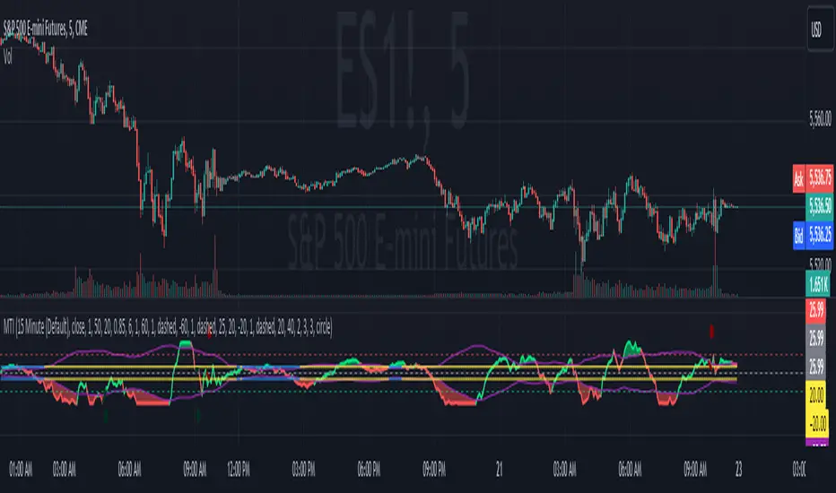
Standard Error Bands**Standard Error Bands Indicator: A Statistically Robust Tool for Trend Analysis**
The Standard Error Bands (SEB) indicator is a powerful technical analysis tool designed to help traders identify and assess trends with greater accuracy. Unlike traditional band indicators (e.g., Bollinger Bands) that rely on price averages, SEB leverages linear regression and statistical measures of volatility to offer deeper insights into market dynamics.
**How It Works**
1. **Linear Regression:** The indicator first calculates a linear regression line to model the underlying price trend. This line represents the "best fit" of price data over the specified lookback period.
2. **Standard Error:** Next, it calculates the standard error of the regression. This statistical measure quantifies the average distance between actual prices and the regression line, effectively acting as a volatility gauge.
3. **Smoothing:** Both the linear regression line and the standard error values are smoothed using a Simple Moving Average (SMA) to reduce noise and enhance the visual clarity of the bands.
4. **Band Construction:** The upper and lower bands are formed by adding/subtracting a multiple of the smoothed standard error from the smoothed linear regression line. The default multiplier is 2, representing approximately 95% of price action expected within the bands under normal market conditions.
**Key Insights**
* **Trend Strength:** Tight bands suggest a strong, well-defined trend with low volatility. Prices tend to adhere closely to the regression line, indicating a high probability of trend continuation.
* **Trend Weakness/Change:** Widening or expanding bands signal increased volatility and potential trend weakness. Prices deviating from the regression line may suggest an impending trend reversal or a shift into a sideways consolidation phase.
* **Entry/Exit Signals:**
* Consider entering a trade when prices break out of the bands in the direction of the trend, especially if the bands were previously tight.
* Conversely, consider exiting a trade when prices pierce the bands against the trend or when the bands start to widen significantly.
**Use Cases**
* **Trend Identification:** SEB can help traders identify trends earlier and more accurately than moving average-based indicators.
* **Trend Confirmation:** The bands can be used to confirm the validity and strength of an existing trend.
* **Volatility Assessment:** Changes in band width provide valuable insights into market volatility, aiding risk management decisions.
* **Entry/Exit Timing:** SEB can be incorporated into trading strategies to generate timely entry and exit signals.
**Important Considerations**
* **Parameter Optimization:** Experiment with different lookback periods, smoothing values, and standard error multipliers to find the optimal settings for your preferred trading style and market conditions.
* **Supplementary Indicators:** Combine SEB with other technical indicators (e.g., momentum oscillators, volume analysis) for a more comprehensive market assessment.
* **Backtesting:** Thoroughly backtest any SEB-based trading strategy to ensure its effectiveness before deploying it in live markets.
**Disclaimer:** Technical indicators like SEB are valuable tools but should not be used in isolation. Always consider price action or fundamental factors and risk management principles when making trading decisions.

Unbound RSIUnbound RSI
Description
The Unbound RSI or de-oscillated RSI indicator is a novel technical analysis indicator that combines the concepts of the Relative Strength Index (RSI) and moving averages, applied directly over the price chart. This indicator is unique in its approach by transforming the oscillatory nature of the RSI into a format that aligns with the price action, thereby offering a distinctive view of market momentum and trends.
Key Features
Multi-Length RSI Analysis: Incorporates three different lengths of RSI (short, medium, and long), providing insights into the momentum and trend strength at various timeframes.
Deoscillation of RSI: The RSI for each length is 'deoscillated' by adjusting its scale to align with the actual price movements. This is achieved by shifting and scaling the RSI values, effectively merging them with the price line.
Average True Range (ATR) Scaling: The deoscillation process includes scaling by the Average True Range (ATR), making the indicator responsive to the asset’s volatility.
Optional Smoothing: Provides an option to apply a simple moving average (SMA) smoothing to each deoscillated RSI line, reducing noise and highlighting more significant trends.
Dynamic Moving Average (MA) Baseline: Features a moving average calculated from the medium length (default value) de-oscillated RSI, serving as a dynamic baseline to identify overarching trends.
How It’s Different
Unlike standard RSI indicators that oscillate in a fixed range, this indicator transforms the RSI to move in tandem with the price, offering a unique perspective on momentum and trend changes. The use of multiple timeframes for RSI and the inclusion of a dynamic MA baseline provide a multifaceted view of market conditions.
Potential Usage
Trend Identification: The position of the price in relation to the different deoscillated RSI lines and the MA baseline can indicate the prevailing market trend.
Momentum Shifts: Crossovers of the price with the deoscillated RSI lines or the MA baseline can signal potential shifts in momentum, offering entry or exit points.
Volatility Awareness: The ATR-based scaling of the deoscillated RSI lines means the indicator adjusts to changes in volatility, potentially offering more reliable signals in different market conditions.
Comparative Analysis: By comparing the short, medium, and long deoscillated RSI lines, traders can gauge the strength of trends and the convergence or divergence of momentum across timeframes.
Best Practices
Backtesting: Given its novel nature, it’s crucial to backtest the indicator across different assets and market conditions.
Complementary Tools: Combine with other technical analysis tools (like support/resistance levels, other oscillators, volume analysis) for more robust trading signals.
Risk Management: Always use sound risk management strategies, as no single indicator provides foolproof signals.

MA RSI @KINGThis Pine Script is designed to create a trading indicator with moving averages (MA) and relative strength index (RSI), along with arrow signals and background color changes based on those signals. Here's a description of its functions:
1. Moving Averages and RSI Calculation:
- Two moving averages (`fastMA` and `slowMA`) are calculated based on user-input lengths.
- The Relative Strength Index (`rsi`) is calculated based on a user-defined length.
2. Crossover Conditions:
- `crossoverUp` is true when the fastMA crosses above the slowMA and RSI is above an overbought level.
- `crossoverDown` is true when the fastMA crosses below the slowMA and RSI is below an oversold level.
3. Arrow Signals:
- Triangle-shaped arrows (`arrowUp` and `arrowDown`) are plotted below and above bars, indicating buy (green) and sell (red) signals, respectively.
4. Background Color Changes:
- The background color (`bgColor`) changes based on buy and sell signals.
- If there's a buy signal (`crossoverUp`), the background color is set to a light blue with 40% transparency.
- If there's a sell signal (`crossoverDown`), the background color is set to a light red with 40% transparency.
- On the next opposite signal, the background color is scaled up (transparency set to 80%) to indicate a stronger signal.
In summary, this script provides visual cues through arrows and background color changes to assist traders in identifying potential buy and sell signals based on moving average crossovers and RSI conditions. The background color variations aim to highlight the strength of the signal, with scaling based on consecutive signals in the same direction.
********************************************************************************
1. Buy Signal:
- Condition: The arrow points up (green) with a background color indicating a buy signal.
- Confirmation: Ensure that there is a strong upward crossover (fastMA above slowMA) and RSI is above the overbought level.
2. Sell Signal:
- Condition: The arrow points down (red) with a background color indicating a sell signal.
- Confirmation: Ensure that there is a strong downward crossover (fastMA below slowMA) and RSI is below the oversold level.
3. Exit Signal:
- Condition: No arrow is present, and the background color is reset.
- Confirmation: Confirm that there is no active buy or sell signal.
Example Trading Rules:
Opening a Long Position (Buy):
- Enter a long (buy) position when:
- The green arrow appears with a light blue background.
- Confirm that the fastMA is above the slowMA.
- Confirm that RSI is above the overbought level.
Opening a Short Position (Sell):
- Enter a short (sell) position when:
- The red arrow appears with a light red background.
- Confirm that the fastMA is below the slowMA.
- Confirm that RSI is below the oversold level.
Exiting a Position:
- Close the position when:
- There is no arrow present (neither green nor red).
- The background color is reset, indicating no active signal.
Risk Management:
Position Sizing: Determine the size of your positions based on your risk tolerance and the size of your trading account.
Stop-Loss and Take-Profit: Set stop-loss orders to limit potential losses and take-profit orders to secure profits.
Risk-Reward Ratio: Consider maintaining a favorable risk-reward ratio in your trades.
Notes:
Backtesting: Before applying this strategy in a live market, it's crucial to backtest it using historical data to assess its performance.
Market Conditions: Adapt the strategy to different market conditions, and be aware that no strategy is guaranteed to be profitable.
Continuous Monitoring: Regularly monitor the performance of the strategy and make adjustments as needed.
Educational Purpose: This strategy is for educational purposes only. Always consult with financial professionals and use your judgment when making trading decisions.
Remember that trading involves risk, and past performance is not indicative of future results. It's recommended to paper trade or use a demo account to test the strategy before risking real capital.
Best wishes on your trading journey! May your strategies be profitable, your risks well-managed, and your decisions guided by wisdom and success. Happy trading!
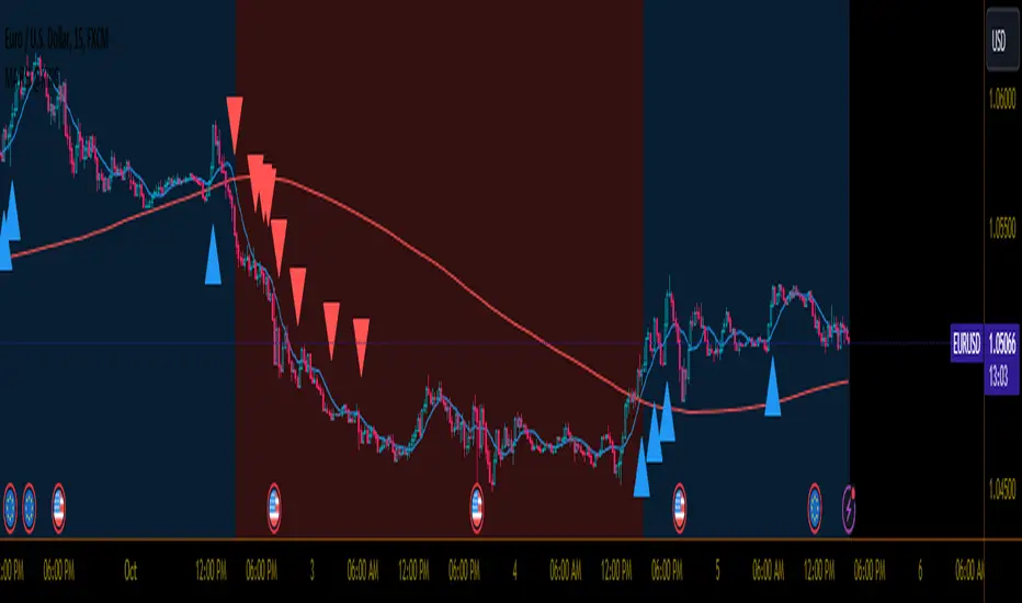
Trend Confirmation StrategyThe profitability and uniqueness of a trading strategy depend on various factors including market conditions, risk management, and the strategy's ability to capitalize on price movements. I'll describe the strategy provided and highlight its potential benefits and differences compared to other strategies:
Strategy Overview:
The provided strategy combines three technical indicators: Supertrend, MACD, and VWAP. It aims to identify potential entry and exit points by confirming trend direction and considering the proximity to the VWAP level. The strategy also incorporates stop-loss and take-profit mechanisms, as well as a trailing stop.
Unique Aspects and Potential Benefits:
Trend Confirmation: The strategy uses both Supertrend and MACD to confirm the trend direction. This dual confirmation can increase the likelihood of accurate trend identification and filter out false signals.
VWAP Confirmation: The strategy considers the proximity of the price to the VWAP level. This dynamic level can act as a support or resistance and provide additional context for entry decisions.
Adaptive Stop Loss: The strategy sets a stop-loss range, which helps provide some tolerance for minor price fluctuations. This adaptive approach considers market volatility and helps prevent premature stop-loss triggers.
Trailing Stop: The strategy incorporates a trailing stop mechanism to lock in profits as the trade moves in the desired direction. This can potentially enhance profitability during strong trends.
Partial Profit Booking: While not explicitly implemented in the provided code, you could consider booking partial profits when the MACD shows a crossover in the opposite direction. This aspect could help secure gains while still keeping exposure to potential further price movements.
Key Differences from Other Strategies:
Dual Indicator Confirmation: The combination of Supertrend and MACD for trend confirmation is a unique aspect of this strategy. It adds an extra layer of filtering to enhance the accuracy of entry signals.
Dynamic VWAP: Incorporating the VWAP level into the decision-making process adds a dynamic element to the strategy. VWAP is often used by institutional traders, and its inclusion can provide insights into the market sentiment.
Adaptive Stop Loss and Trailing: The strategy's use of an adaptive stop-loss range and a trailing stop can help manage risk and protect profits more effectively during changing market conditions.
Partial Profit Booking: The suggestion to consider partial profit booking upon MACD crossovers in the opposite direction is a practical approach to secure gains while staying in the trade.
Caution and Considerations:
Backtesting: Before deploying any strategy in real trading, it's crucial to thoroughly backtest it on historical data to understand its performance under various market conditions.
Risk Management: While the strategy has built-in risk management mechanisms, it's essential to carefully manage position sizes and overall portfolio risk.
Market Conditions: No strategy works well in all market conditions. It's important to be flexible and adjust the strategy or refrain from trading during particularly volatile or unpredictable periods.
Continuous Monitoring: Even though the strategy includes automated components, continuous monitoring of the trades and market conditions is necessary.
Adaptability: Markets can change over time. Traders need to be prepared to adapt the strategy as necessary to stay aligned with evolving market dynamics.

Athena Momentum Squeeze - Short, Lean, and Mean This is a very profitable strategy focusing on 15 minute intervals on the Micro Nasdaq Futures contracts. CME_MINI:MNQH2023
As this contract only keeps positions for on average about an hour risk is managed. At a profit factor of 3.382 with a max drawdown of $123 from January 1st to February 15. Looking back to Dec 2019 still maintains a profit factor of 1.3.
See backtesting: www.screencast.com
2019 backtesting: www.screencast.com
Based on the classic Lazy Bear Oscillator Squeeze with a number of modifications from ADX, MAs and adding fibonacci levels.
We like keeping strategies simple yet powerful, no completely where you can't understand your own trades.
Our team is always modifying and improving the strategy. Always open to collaborating on improving as there is no perfect strategy. www.screencast.com
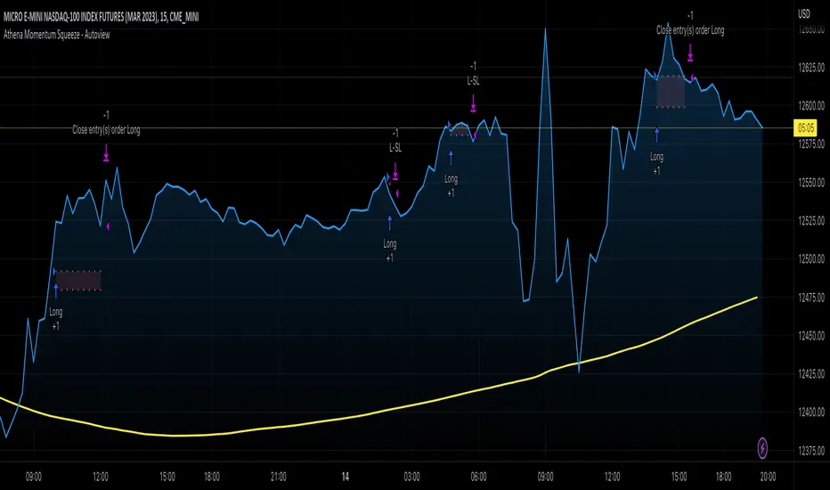
DR/IDR Case Study [TFO]This indicator was made to backtest the DR / IDR concept (Defining Range / Implied Defining Range). There is only one built in DR session, but it can be changed to fit whatever session you like. Just make sure that the beginning time of the Session parameter matches the end time of the Defining Range parameter.
I'm not trying to validate or invalidate the claims of the DR concept, as the sample size of the success rate from this indicator is likely significantly smaller than that of the backtests where the initial success rates were derived. I'm simply sharing this indicator to encourage others to do their own due diligence by collecting their own data before implementing new concepts in their trading. Likewise I'm also making this open source for those who wish to do different kinds of backtesting and extract more value from this concept - for example, what percentage of the time does the session actually close further from the DR after initially closing through the range? Data like this could be good to track for those looking to make a trading model out of the DR concept.
Please note that all times are set to the "America/New_York" time zone by default. Besides the fact that the input times will use New York local time, this also means that they automatically adjust for Daylight Savings (this only impacts areas that do not observe Daylight Savings).

Weird Renko StratThis strategy uses Renko, it generates a signal when there is a reversal in Renko. When using historical data, it provides a good entry and an okay exit. However, in a real-time environment, this strategy is subject to repaint and may produce a false signal.
As a result, the backtesting result should not be used as a metric to predict future results. It is highly recommended to forward-test the strategy before using it in real trading. I forward test it from 12/18/2022 to 12/21/2022 in paper trading, using the alert feature in Tradingview. I made 60 trades trading the BTCUSDT BINANCE 3 min with 26 as the param and under the condition that I use 20x margin, compounding my yield, and having 0 trading fee, a steady loss is generated: from $10 to $3.02.
This is quite interesting. As if I flip the signal from "Long" to "Short" and another way too, it will be a steady profit from $10 to $21.85. Hence, if I'm trying to anti-trade the real-time alert signal, the current "4 Days Result" will be good. Nevertheless, I still have to forward-test it for longer to see if it will fail eventually.
Dive into the setting of the strategy
- Margin is the leverage you use. 1 means 1x, 10 means 10x. It affects the backtest yield when you backtest
- Compound Yield button is for compound calculation, disable it to go back to normal backtesting
- Anti Strategy button is to do the opposite direction trade, when the original strat told you to "Long", you "Short" instead. Enable it to use the feature
- Param is the block size for the Renko chart
- Drawdown is just a visual tool for you in case you want to place a stop loss (represent by the semitransparent red area in the chart)
- From date Thru Date is to specify the backtest range of the strategy, This feature is turned off by default. It is controlled by the Max Backtest Timeframe which will be explain below
- Max Backtest Timeframe control the From date Thru Date function, disable it to enable the From Date Thru Date function
Param is the most important input in this strategy as it directly affects performance. It is highly recommended to backtest nearly all the possible parameters before deploying it in real trading. Some factors should be considered:
- Price of the asset (like an asset of 1 USD vs an asset of 10000 USD required different param)
- Timeframe (1-minute param is different than 1-month param)
I believe this is caused by the volatility of the selected timeframe since different timeframe has different volatility. Param should be fine-tuned before usage.
Here is the param I'm using:
BTCUSDT BINANCE 3min: 26
BTCUSDT BINANCE 5min: 28
BTCUSDT BINANCE 1day: 15
Background of the strategy:
- The strategy starts with $10 at the start of backtesting (customizable in setting)
- The trading fee is set to 0.00% which is not common for most of the popular exchanges (customizable in setting)
- The contract size is not a fixed amount, but it uses your balance to buy it at the open price. If you are using the compound mode, your balance will be your current total balance. If you are using the non-compound mode, it will just use the $10 you start with unless you change the amount you start with. If you are using a margin higher than 1, it will calculate the corresponding contract size properly based on your margin. (Only these options are allowed, you are not able to change them without changing the code)
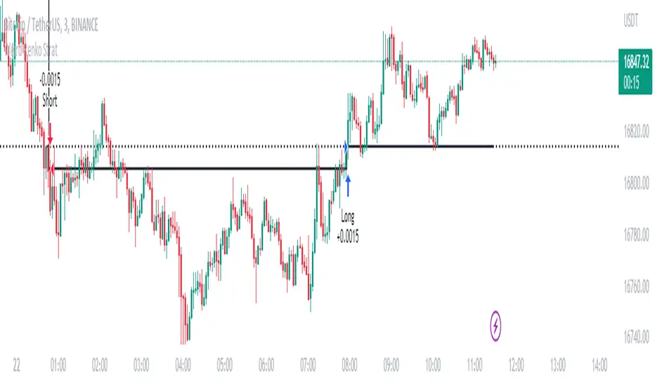
Pinescript v4 - The Holy Grail (Trailing Stop)After studying several other scripts, I believe I have found the Holy Grail! (Or perhaps I've just found a bug with Tradingview's Pinescript v4 language) Anyhow, I'm publishing this script in the hope that someone smarter than myself could shed some light on the fact that adding a trailing stop to any strategy seems to make it miraculously...no that's an understatement...incredulously, stupendously, mind-bendingly profitable. I'm talking about INSANE profit factors, higher than 200x, with drawdowns of <10%. Sounds too good to be true? Maybe it is...or you could hook it up to your LIVE broker, and pray it doesn't explode. This is an upgraded version of my original Pin Bar Strategy.
Recommended Chart Settings:
Asset Class: Forex
Time Frame: H1
Long Entry Conditions:
a) Exponential Moving Average Fan up trend
b) Presence of a Bullish Pin Bar
c) Pin Bar pierces the Exponential Moving Average Fan
Short Entry Conditions:
a) Exponential Moving Average down trend
b) Presence of a Bearish Pin Bar
c) Pin Bar pierces the Exponential Moving Average Fan
Exit Conditions:
a) Trailing stop is hit
b) Moving Averages cross-back (optional)
c) It's the weekend
Default Robot Settings:
Equity Risk (%): 3 //how much account balance to risk per trade
Stop Loss (x*ATR, Float): 0.5 //stoploss = x * ATR, you can change x
Stop Loss Trail Points (Pips): 1 //the magic sauce, not sure how this works
Stop Loss Trail Offset (Pips): 1 //the magic sauce, not sure how this works
Slow SMA (Period): 50 //slow moving average period
Medium EMA (Period): 18 //medium exponential moving average period
Fast EMA (Period): 6 //fast exponential moving average period
ATR (Period): 14 // average true range period
Cancel Entry After X Bars (Period): 3 //cancel the order after x bars not triggered, you can change x
Backtest Results (2019 to 2020, H1, Default Settings):
AUDUSD - 1604% profit, 239.6 profit factor, 4.9% drawdown (INSANE)
NZDUSD - 1688.7% profit, 100.3 profit factor, 2.5% drawdown
GBPUSD - 1168.8% profit, 98.7 profit factor, 0% drawdown
USDJPY - 900.7% profit, 93.7 profit factor, 4.9% drawdown
USDCAD - 819% profit, 31.7 profit factor, 8.1% drawdown
EURUSD - 685.6% profit, 26.8 profit factor, 5.9% drawdown
USDCHF - 1008% profit, 18.7 profit factor, 8.6% drawdown
GBPJPY - 1173.4% profit, 16.1 profit factor, 7.9% drawdown
EURAUD - 613.3% profit, 14.4 profit factor, 9.8% drawdown
AUDJPY - 1619% profit, 11.26 profit factor, 9.1% drawdown
EURJPY - 897.2% profit, 6 profit factor, 13.8% drawdown
EURGBP - 608.9% profit, 5.3 profit factor, 9.8% drawdown (NOT TOO SHABBY)
As you can clearly see above, this forex robot is projected by the Tradingview backtester to be INSANELY profitable for all common forex pairs. So what was the difference between this strategy and my previous strategies? Check my code and look for "trail_points" and "trail_offset"; you can even look them up in the PineScript v4 documentation. They specify a trailing stop as the exit condition, which automatically closes the trade if price reverses against you.
I however suspect that the backtester is not properly calculating intra-bar price movement, and is using a simplified model. With this simplfied approach, the trailing stop code becomes some sort of "holy grail" generator, making every trade entered profitable.
Risk Warning:
This is a forex trading strategy that involves high risk of equity loss, and backtest performance will not equal future results. You agree to use this script at your own risk.
Hint:
To get more realistic results, and *maybe* overcome the intrabar simulation error, change the settings to: "Stop Loss Trail Points (pips)": 100
I am not sure if this eradicates the bug, but the entries and exits look more proper, and the profit factors are more believable.

TrendMaAlignmentStrategy - Long term tradesThis is another strategy based on moving average alignment and HighLow periods. This is more suitable for long term trend traders and mainly for stocks.
Candle is colored lime if : Lookback Period has at least one bar with moving averages fully aligned OR None of the bars in Lookback periods has negatively aligned moving averages (More than half are positively aligned).
Candle is colored orange if : Lookback Period has at least one bar with moving averages fully aligned in negative way OR none of the bars in lookback has positively aligned moving averages (More than half are negatively aligned).
If either of above conditions are met, candle is colored silver.
Moving average alignment parameters:
Moving Average Type : MA Type for calculating Aligned Moving Average Index
Lookback Period : Lookback period to check highest and lowest Moving Average index.
HighLow parameters:
Short High/Low Period: Short period to check highs and lows
Long High/Low Period: Longer Period to check highs and lows.
If short period high == long period high, which means, instrument has made new high in the short period.
ATR Parameters:
ATR Length: ATR periods
StopMultiplyer: To set stop loss.
ReentryStopMultiplyer: This is used when signal is green buy stop loss on previous trade is hit. In such cases, new order will not be placed until it has certain distance from stop line.
Trade Prameters:
Exit on Signal : To be used with caution. Enabling it will allow us to get out on bad trades early and helps exit trades in long consolidation periods. But, this may also cause early exit in the trend. If instrument is trending nicely, it is better to keep this setting unchecked.
Trade direction : Default is long only. Short trades are not so successful in backtest. Use it with caution.
Backtest years : limit backtesting to certain years.
Part of the logic used from study's below:
Other strategies based on these two studies are below (which are meant for short - medium terms):

Forward testing code block by CanundoThis is purely a code block useable for strategies you want to forward test. No backtest will happen.
It's especially important to figure out if a strategy will perform as well in live trading as it does in backtesting since the trades in backtests are calculated differently. It can be a great difference.
It's best to test it on 1 minute timeframe or lower. It would take 1-2 minutes to see the first trade happen while no trade before exists.

Relative StrengthThis strategy employs a custom "strength" function to assess the relative strength of a user-defined source (e.g., closing price, moving average) compared to its historical performance over various timeframes (8, 34, 20, 50, and 200 periods). The strength is calculated as a percentage change from an Exponential Moving Average (EMA) for shorter timeframes and a Simple Moving Average (SMA) for longer timeframes. Weights are then assigned to each timeframe based on a logarithmic scale, and a weighted average strength is computed.
Key Features:
Strength Calculation:
Calculates the relative strength of the source using EMAs and SMAs over various timeframes.
Assigns weights to each timeframe based on a logarithmic scale, emphasizing shorter timeframes.
Calculates a weighted average strength for a comprehensive view.
Visualizations:
Plots the calculated strength as a line, colored green for positive strength and red for negative strength.
Fills the background area below the line with green for positive strength and red for negative strength, enhancing visualization.
Comparative Analysis:
Optionally displays the strength of Bitcoin (BTC), Ethereum (ETH), S&P 500, Nasdaq, and Dow Jones Industrial Average (DJI) for comparison with the main source strength.
Backtesting:
Allows users to specify a start and end time for backtesting the strategy's performance.
Trading Signals:
Generates buy signals when the strength turns positive from negative and vice versa for sell signals.
Entry and exit are conditional on the backtesting time range.
Basic buy and sell signal plots are commented out (can be uncommented for visual representation).
Risk Management:
Closes all open positions and cancels pending orders outside the backtesting time range.
Disclaimer:
Backtesting results do not guarantee future performance. This strategy is for educational purposes only and should be thoroughly tested and refined before risking capital.
Additional Notes:
- The strategy uses a custom "strength" function that can be further customized to explore different timeframes and weighting schemes.
- Consider incorporating additional technical indicators or filters to refine the entry and exit signals.
- Backtesting with different parameters and market conditions is crucial for evaluating the strategy's robustness.
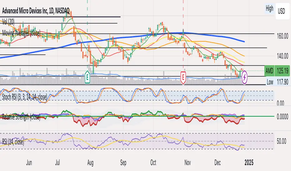
Price Action Analyst [OmegaTools]Price Action Analyst (PAA) is an advanced trading tool designed to assist traders in identifying key price action structures such as order blocks, market structure shifts, liquidity grabs, and imbalances. With its fully customizable settings, the script offers both novice and experienced traders insights into potential market movements by visually highlighting premium/discount zones, breakout signals, and significant price levels.
This script utilizes complex logic to determine significant price action patterns and provides dynamic tools to spot strong market trends, liquidity pools, and imbalances across different timeframes. It also integrates an internal backtesting function to evaluate win rates based on price interactions with supply and demand zones.
The script combines multiple analysis techniques, including market structure shifts, order block detection, fair value gaps (FVG), and ICT bias detection, to provide a comprehensive and holistic market view.
Key Features:
Order Block Detection: Automatically detects order blocks based on price action and strength analysis, highlighting potential support/resistance zones.
Market Structure Analysis: Tracks internal and external market structure changes with gradient color-coded visuals.
Liquidity Grabs & Breakouts: Detects potential liquidity grab and breakout areas with volume confirmation.
Fair Value Gaps (FVG): Identifies bullish and bearish FVGs based on historical price action and threshold calculations.
ICT Bias: Integrates ICT bias analysis, dynamically adjusting based on higher-timeframe analysis.
Supply and Demand Zones: Highlights supply and demand zones using customizable colors and thresholds, adjusting dynamically based on market conditions.
Trend Lines: Automatically draws trend lines based on significant price pivots, extending them dynamically over time.
Backtesting: Internal backtesting engine to calculate the win rate of signals generated within supply and demand zones.
Percentile-Based Pricing: Plots key percentile price levels to visualize premium, fair, and discount pricing zones.
High Customizability: Offers extensive user input options for adjusting zone detection, color schemes, and structure analysis.
User Guide:
Order Blocks: Order blocks are significant support or resistance zones where strong buyers or sellers previously entered the market. These zones are detected based on pivot points and engulfing price action. The strength of each block is determined by momentum, volume, and liquidity confirmations.
Demand Zones: Displayed in shades of blue based on their strength. The darker the color, the stronger the zone.
Supply Zones: Displayed in shades of red based on their strength. These zones highlight potential resistance areas.
The zones will dynamically extend as long as they remain valid. Users can set a maximum number of order blocks to be displayed.
Market Structure: Market structure is classified into internal and external shifts. A bullish or bearish market structure break (MSB) occurs when the price moves past a previous high or low. This script tracks these breaks and plots them using a gradient color scheme:
Internal Structure: Short-term market structure, highlighting smaller movements.
External Structure: Long-term market shifts, typically more significant.
Users can choose how they want the structure to be visualized through the "Market Structure" setting, choosing from different visual methods.
Liquidity Grabs: The script identifies liquidity grabs (false breakouts designed to trap traders) by monitoring price action around highs and lows of previous bars. These are represented by diamond shapes:
Liquidity Buy: Displayed below bars when a liquidity grab occurs near a low.
Liquidity Sell: Displayed above bars when a liquidity grab occurs near a high.
Breakouts: Breakouts are detected based on strong price momentum beyond key levels:
Breakout Buy: Triggered when the price closes above the highest point of the past 20 bars with confirmation from volume and range expansion.
Breakout Sell: Triggered when the price closes below the lowest point of the past 20 bars, again with volume and range confirmation.
Fair Value Gaps (FVG): Fair value gaps (FVGs) are periods where the price moves too quickly, leaving an unbalanced market condition. The script identifies these gaps:
Bullish FVG: When there is a gap between the low of two previous bars and the high of a recent bar.
Bearish FVG: When a gap occurs between the high of two previous bars and the low of the recent bar.
FVGs are color-coded and can be filtered by their size to focus on more significant gaps.
ICT Bias: The script integrates the ICT methodology by offering an auto-calculated higher-timeframe bias:
Long Bias: Suggests the market is in an uptrend based on higher timeframe analysis.
Short Bias: Indicates a downtrend.
Neutral Bias: Suggests no clear directional bias.
Trend Lines: Automatic trend lines are drawn based on significant pivot highs and lows. These lines will dynamically adjust based on price movement. Users can control the number of trend lines displayed and extend them over time to track developing trends.
Percentile Pricing: The script also plots the 25th percentile (discount zone), 75th percentile (premium zone), and a fair value price. This helps identify whether the current price is overbought (premium) or oversold (discount).
Customization:
Zone Strength Filter: Users can set a minimum strength threshold for order blocks to be displayed.
Color Customization: Users can choose colors for demand and supply zones, market structure, breakouts, and FVGs.
Dynamic Zone Management: The script allows zones to be deleted after a certain number of bars or dynamically adjusts zones based on recent price action.
Max Zone Count: Limits the number of supply and demand zones shown on the chart to maintain clarity.
Backtesting & Win Rate: The script includes a backtesting engine to calculate the percentage of respect on the interaction between price and demand/supply zones. Results are displayed in a table at the bottom of the chart, showing the percentage rating for both long and short zones. Please note that this is not a win rate of a simulated strategy, it simply is a measure to understand if the current assets tends to respect more supply or demand zones.
How to Use:
Load the script onto your chart. The default settings are optimized for identifying key price action zones and structure on intraday charts of liquid assets.
Customize the settings according to your strategy. For example, adjust the "Max Orderblocks" and "Strength Filter" to focus on more significant price action areas.
Monitor the liquidity grabs, breakouts, and FVGs for potential trade opportunities.
Use the bias and market structure analysis to align your trades with the prevailing market trend.
Refer to the backtesting win rates to evaluate the effectiveness of the zones in your trading.
Terms & Conditions:
By using this script, you agree to the following terms:
Educational Purposes Only: This script is provided for informational and educational purposes and does not constitute financial advice. Use at your own risk.
No Warranty: The script is provided "as-is" without any guarantees or warranties regarding its accuracy or completeness. The creator is not responsible for any losses incurred from the use of this tool.
Open-Source License: This script is open-source and may be modified or redistributed in accordance with the TradingView open-source license. Proper credit to the original creator, OmegaTools, must be maintained in any derivative works.