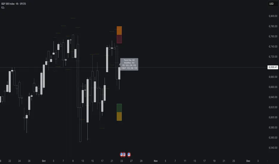
Reversal Zones// This indicator identifies likely reversal zones above and below current price by aggregating multiple technical signals:
// • Prior Day High/Low
// • Opening Range (9:30–10:00)
// • VWAP ±2 standard deviations
// • 60‑minute Bollinger Bands
// It draws shaded boxes for each base level, then computes a single upper/lower reversal zone (closest level from combined signals),
// with configurable zone width based on the expected move (EM). Within those reversal zones, it highlights an inner “strike zone”
// (percentage of the box) to suggest optimal short-option strikes for credit spreads or iron condors.
// Additional features:
// • Optional Expected Move lines from the RTH open
// • 15‑minute RSI/Mean‑Reversion and Trend‑Day confluence flags displayed in a dashboard
// • Toggles to include/exclude each signal and adjust styling
// How to use:
// 1. Adjust inputs to select which levels to include and set the expected move parameters.
// 2. Reversal boxes (red above, green below) show zones where price is most likely to reverse.
// 3. Inner strike zones (darker shading) guide optimal short-strike placement.
// 4. Dashboard confirms whether mean-reversion or trend-day conditions are active.
// Customize colors and visibility in the settings panel. Enjoy disciplined, confluence-based trade entries!
Cari dalam skrip untuk "band"
Institutional Rolling VWAPs • 3 lines + editable σ bands3 rolling vwaps, time stamped, same on htf and lft for high level execution

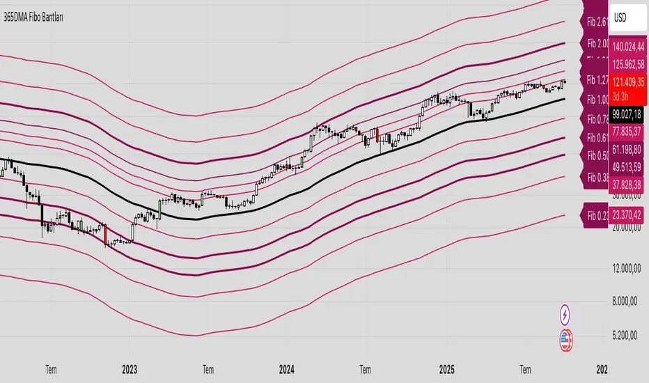
365 DMA Based Multiplier Fibonacci BandsBitcoin Chart
365 DMA Based
Fibonacci 1.0 = Long term trend
Fibonacci 0.5/0.618 = Long term support
Fibonacci 1.618 = Mid term target
Fibonacci 2.618 = Long term target
MA Paketi This advanced MA & ATR Channel Indicator allows you to monitor both short-term and long-term trends on the same chart.
The script includes 9, 21, 50, 100, and 200-period moving averages (MAs) and also lets you add a custom MA of your choice.
Around the 200 MA, a ±6 ATR channel dynamically defines volatility-based support and resistance zones.
Key Features:
🔹 Five classic MAs (9, 21, 50, 100, 200)
🔹 User-defined custom MA (SMA, EMA, WMA, RMA, HMA options)
🔹 MA200-centered ±ATR channel (fully adjustable multiplier and period)
🔹 ATR-based dynamic volatility band
🔹 Alert conditions (notifies when price breaks above or below the channel)
🔹 Clean, colorful, and professional visual design
This indicator helps you analyze trend direction, momentum shifts, and volatility-driven reversal zones simultaneously.
Perfect for swing, scalp, and position traders alike.


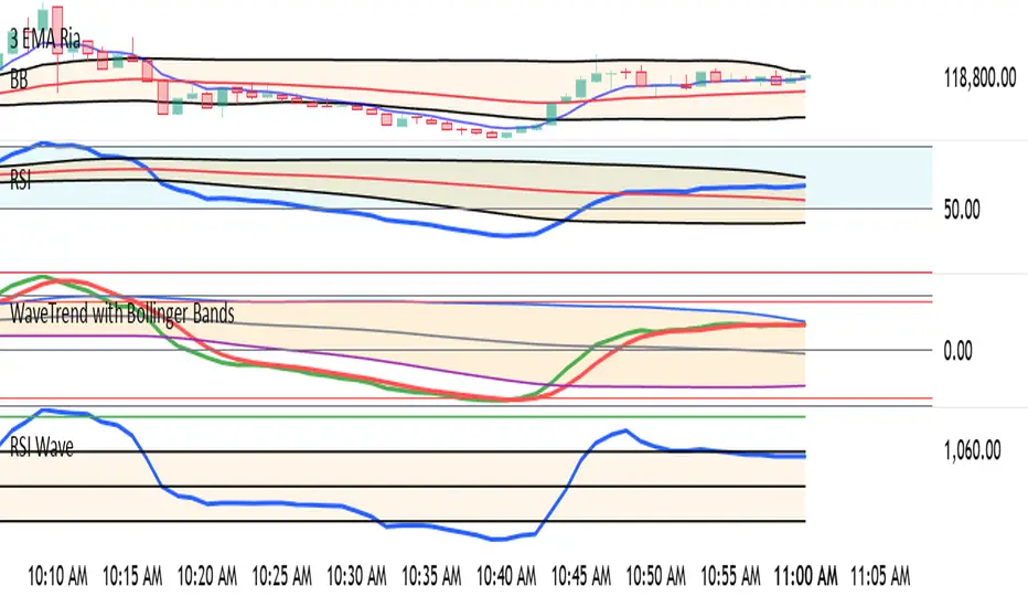
WaveTrend with Bollinger BandsPlots TTM Squeeze momentum histogram (green/red).
Plots RSI (blue) in the same pane.
Shows squeeze dots and RSI overbought/oversold lines.
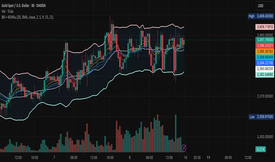
BB + 4 EMAsCustom Bollinger Bands with 4EMAs of your choice. All added in one indicator.
Look Before You Leap!

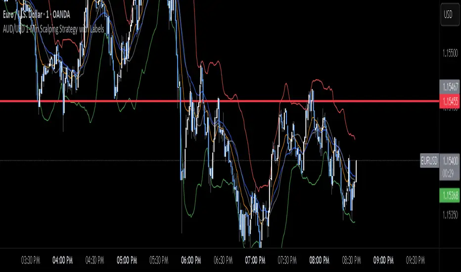
AUD/USD 1-Min Scalping Strategy with LabelsHere’s a complete TradingView Pine Script v5 for the 1-minute AUD/USD scalping strategy we just discussed. This strategy uses:
EMA 13 and EMA 26 for trend filtering
Bollinger Bands for volatility extremes
RSI (4) for momentum confirmation
Double Bollinger Bands - SF2000twin BB's. One bb can be set for , eg 20 period. The other set for - eg - 50 period. compare the channels.
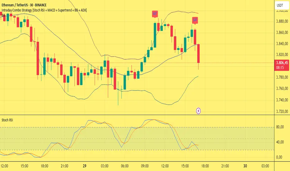
Intraday Combo Strategy HHStochastic RSI Momentum/Reversal quickly identifies overbought/oversold zones
MACD Momentum/Trend confirms a trend reversal, a late but powerful signal
Supertrend Trend Tracking provides clear and concise buy/sell signals
Bollinger Bands Volatility shows price deviation during breakouts/squeezes
ADX Trend Strength measures trend strength to filter out false signals
AWR_8DLRC1. Overview and Objective
The AWR_8DLRC indicator is designed to display multiple dynamic channels directly on your chart (with the overlay enabled). It creates dynamic envelopes based on a regression-like approach combined with a volatility measure derived from the root mean square error (RMSE). These channels can help identify support and resistance areas, overbought/oversold conditions, or even potential trend reversals by providing several layers of analysis using different multipliers and timeframes.
2. Input Parameters
Source and Multiplier
The indicator uses the closing price (close) as its default data source.
A floating-point parameter mult (default value: 3.0) is available. This multiplier is primarily used for channel 5, while other channels employ fixed multipliers (1, 2, or 3) to generate different sensitivity levels.
Channel Lengths
Several channels are calculated with distinct lookback lengths:
Channel 5: Uses a length of 1000 periods (its plot is commented out in the code, so it is not displayed by default).
Channel 6: Uses a length of 2000 periods.
Channel 7: Uses a length of 3000 periods.
Channel 8: Uses a length of 4000 periods.
Custom Colors and Transparencies
Each channel (or group of channels) can be customized with specific colors and transparency settings. For example, channel 6 uses a light yellow tone, channel 7 is red, and channel 8 is white.
Additionally, specific fill colors are defined for the shaded areas between the upper and lower lines of some channels, enhancing visual clarity.
3. Channel Calculation Mechanism
At the heart of the indicator is the function f_calcChannel(), which takes as input:
A data source (_src),
A period (_length), and
A multiplier (_mult).
The calculation process comprises several key steps:
Moving Averages Calculation
The function computes both a weighted moving average (WMA) and a simple moving average (SMA) over the defined length.
Baseline Determination
It then combines these averages into two values (A and B) using linear formulas (e.g., A = 4*b - 3*a and B = 3*a - 2*b). These values help to establish a baseline that represents the central trend during the lookback period.
Slope and Deviation Calculation
A slope (m) is calculated based on the difference between A and B.
The function iterates over the period, measuring the squared deviation between the actual data point and a corresponding value on the regression line. The sum of these squared deviations is used to compute the RMSE.
Defining Upper and Lower Bounds
The RMSE is multiplied by the provided multiplier (_mult) and then added to or subtracted from the baseline B to create the upper and lower channel boundaries.
This method produces an envelope that widens or narrows based on the volatility reflected by the RMSE.
This process is repeated using different multipliers (1, 2, and 3) for channels 6, 7, and 8, providing multiple levels that offer deeper insights into market conditions.
4. Chart Visualization
The indicator plots several lines and shaded regions:
Channels 6, 7, and 8: For each of these channels, three levels are calculated:
Levels with a multiplier of 1 (thin lines with a line width of 1),
Levels with a multiplier of 2 (medium lines with a line width of 2),
Levels with a multiplier of 3 (thick lines with a line width of 4).
To further enhance visual interpretation, shaded areas (fills) are added between the upper and lower lines — notably for the level with multiplier 3.
Channel 5: Although the calculations for channel 5 are included, its plot commands are commented out. This means it won’t display on the chart unless you uncomment the relevant lines by modifying the script.
5. Conditions and Alerts
Beyond the visual channels, the indicator integrates several alert conditions and visual markers:
Graphical Conditions:
The script defines conditions checking whether the price (i.e., the source) is above or below specific channel levels, particularly the levels calculated with multipliers 2 and 3.
“Mixed” conditions are also established to detect when the price is simultaneously above one set of levels and below another, aiming to highlight potential reversal areas.
Automated Alerts:
Alert conditions are programmed to notify you when the price crosses specific channel boundaries:
Alerts for conditions such as “Upper Channels 2” or “Lower Channels 2” indicate when prices exceed or fall below the second level of the channels.
Similarly, alerts for “Upper Channels 3” and “Lower Channels 3” correspond to the more extreme boundaries defined by the multiplier of 3.
Visual Symbols:
The indicator employs the plotchar() function to place symbols (like 🌙, ⚠️, 🪐, and ☢️) directly on the chart. These symbols make it easy to spot when the price meets these crucial levels.
These alert features are especially valuable for traders who rely on real-time notifications to adjust positions or watch for potential trend shifts.
6. How to Use the Indicator
Installation and Setup:
Copy the provided code into your Pine Script editor on your charting platform (e.g., TradingView) and add the indicator to your chart.
Customize the parameters according to your trading strategy:
Channel Lengths: Modify the lookback periods to see how the envelope adapts.
Colors and Transparencies: Adjust these to fit your display preferences.
Multipliers: Experiment with the multipliers to observe how different settings affect the channel widths.
Interpreting the Channels:
The upper and lower bands represent dynamic thresholds that change with market volatility.
A price that nears an upper boundary might indicate an overextended move upward, whereas a break beyond these dynamic boundaries could signal a potential trend reversal.
Utilizing Alerts:
Configure notifications based on the alert conditions so you can be alerted when the price moves beyond the defined channel levels. This can help trigger entry or exit signals, or simply keep you informed of significant price movements.
Multi-Level Analysis:
The strength of this indicator lies in its multi-level approach. With three defined levels for channels 6, 7, and 8, you gain a more nuanced view of market volatility and trend strength.
For instance, a price crossing the level with a multiplier of 2 might indicate the start of a trend change, while a break of the level with multiplier 3 might confirm a strong trend movement.
7. In Summary
The AWR_8DLRC indicator is a comprehensive tool for drawing dynamic channels based on a regression and RMSE-driven volatility measure. It offers:
Multiple channel levels, each with different lookback periods and multipliers.
Shaded regions between channel boundaries for rapid visual interpretation.
Alert conditions to notify you immediately when the price hits critical levels.
Visual markers directly on the chart to highlight key moments of price action.
This indicator is particularly suited for technical traders seeking to dynamically identify support and resistance zones with a responsive alert system. Its customizable settings and rich array of signals provide an excellent framework to refine your trading decisions.

VWAP Z-Score Oscillator + Scaled TableVWAP Z-Score Oscillator + Scaled Table
This indicator calculates the Z-Score of the VWAP (Volume Weighted Average Price) based on your chosen source price and reset period (Session, Week, Month, Quarter, or Year).
The Z-Score represents how many standard deviations the current price is from the VWAP, visualized as an oscillator oscillating between ±3 sigma levels. The indicator also features three standard deviation bands for easy reference.
To enhance readability, a scaled Z-Score is displayed in a clean, minimalistic table on the top right of the indicator panel. This score is linearly capped between -2 and +2, mapping the raw Z-Score values with limits at ±3 sigma for clarity and quick assessment.
Use this tool to identify extreme deviations from the VWAP, which may signal potential reversals or continuation of price trends.

Turtle ZoneTurtle Zone indicator helps to visually determine support and resistance zones of the price movement.
Displays a channel with zones located symmetrically around the moving average of the price.
Width of the channel is determined by the current volatility computed as average true range which makes the channel width adaptable to the volatility.
Touching of the zones from inside of the channel can be interpreted as a signal of potential reversal.
Breaking outside of the outer boundary of the zones can be interpreted as a signal of a potential continuation of price movement.
Parameters
• Price Source - Component of the bar for computation. Default is ‘hlc3’. Other reasonable values, such as ‘ohlc4’, ‘open’ or’ close’ can be used by advanced users.
• Lookback period - Amount of bars used in moving average computation. Default is 200.
• Inner Amplitude - Relative width of the inner channel. Default is 5.6.
• Outer Amplitude - Relative width of the outer channel. Default is 9.6.
Available plots for notifications
There are five plots on the graph comprising the channel: four boundaries of the channel bands and one hidden mean line of the channel:
Upper Zone Upper Line
Upper Zone Lower Line
Mean
Lower Zone Upper Line
Lower Zone Lower Line
All of the plots can be used to set up notifications.
Notes
All computations are performed in logarithmic price scale which makes this indicator useful on large timeframes.
Credits
This script uses Ehlers_Super_Smoother library by KevanoTrades

Upper and Lower bound for pairs/BTCUpper and Lower Bound for Pairs/BTC
This indicator provides dynamic upper and lower boundary levels for cryptocurrency pairs traded against BTC. It uses statistical or technical analysis methods, such as Z-Score, Bollinger Bands, or moving averages, to identify key resistance (upper bound) and support (lower bound) levels.
Key Features:
Dynamic Boundaries: Tracks real-time price fluctuations of selected pairs against BTC, adapting to market conditions.
Market Insights: Helps traders visualize potential overbought (upper bound) and oversold (lower bound) zones for pairs like ETH/BTC, DOGE/BTC, and others.
Customizable Settings: Allows users to configure lookback periods, standard deviations, or other parameters for boundary calculations.
Decision Support: Assists in identifying reversal or breakout points to refine entry and exit strategies.
This tool is ideal for traders seeking to optimize risk management and spot opportunities in BTC pair markets.

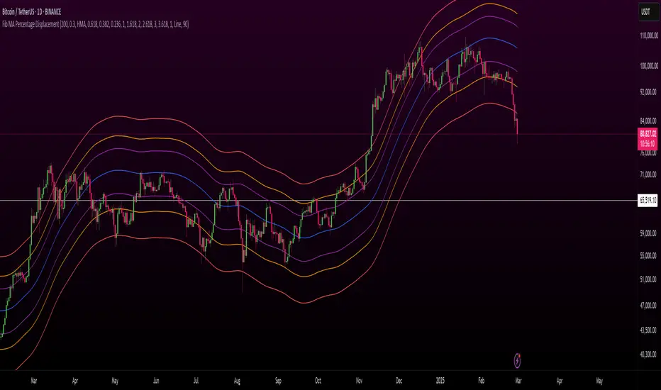
Fibonacci Displaced Moving Averages with Percentage DisplacementThis indicator combines Fibonacci levels with percentage-based displacement, creating a versatile tool for analyzing moving averages in relation to market trends and potential reversal points. It's designed to adapt to different market conditions and asset types, making it a valuable addition to a trader's toolkit.
Key Features:
Fibonacci-Infused Averages: Leverages Fibonacci ratios (0.618, 0.382, 0.236) to construct displaced moving averages. This method offers a layered perspective of market support and resistance levels.
Adaptive Percentage-Based Displacement: The displacement of the moving average is calculated as a percentage of the average, allowing for flexible and market-responsive band positioning. This feature is particularly crucial for adapting to the unique volatility and price behavior of different trading pairs.
Customizable SMA Core: The core of the indicator is a simple moving average (SMA), which can be tailored in length to suit various trading strategies and timeframes.
Logarithmic Scale Compatibility: Includes an option for logarithmic scaling, making it applicable to a broad range of assets, including those with exponential price trends.
Advanced Alert System: Equipped with a comprehensive alert system, it notifies traders of price crossings over any of the Fibonacci displaced moving averages, aiding timely market responses.
Optimizing for Different Pairs:
To maximize the indicator's effectiveness, it is crucial to fine-tune the Percentage Displacement setting according to the specific volatility and price movement characteristics of each trading pair. This customization ensures that the displaced moving averages accurately reflect the market dynamics of each asset, providing more reliable support and resistance levels for traders.
Ideal Use Cases:
This indicator is ideal for traders who seek a deeper understanding of moving averages, especially in markets where Fibonacci levels play a significant role. It is versatile enough for various trading approaches, including swing and day trading, and adaptable across multiple timeframes.
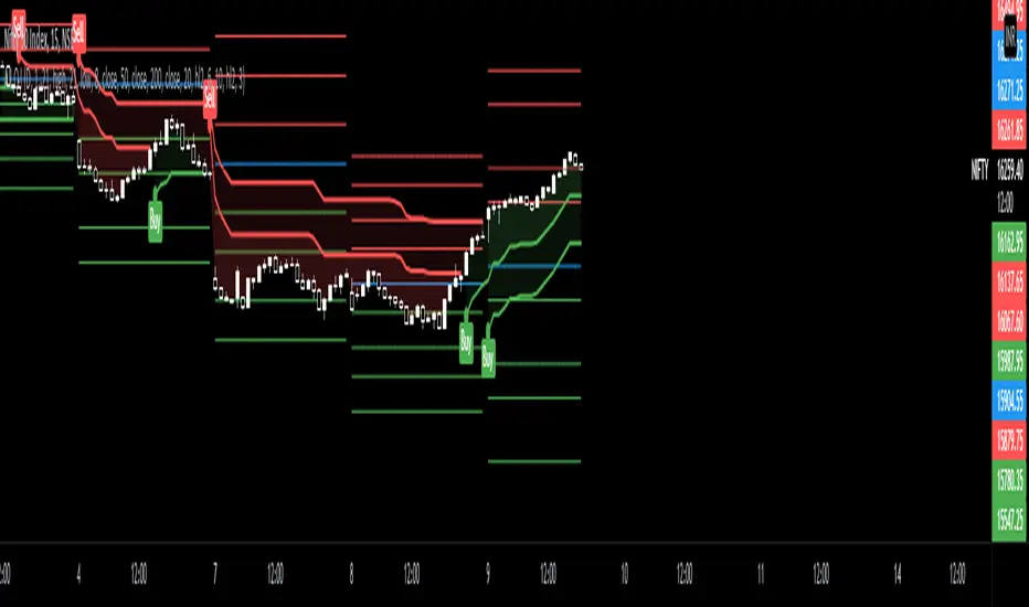
Thursday Close BandsThis script is useful for Indian Markets where weekly expiry is on Thursday.
As per last 10 years historical stats Nifty stays with in 3% range from Thursday close 80% times.

BB Strategy toobabollinger bands strategy with added upper basis and lower line on the chart.
when we use BB strategy in trading view unfortunately the upper, lower and basis line did not display.
so we solve the problem with just a little script codes and bring back the lines to the chart

MCL-YG Pair Trading StrategyThis strategy uses Bollinger Band breakouts to detect buy and sell signals on a correlated pair of assets.


Joker Linear Regression ChannelLinear regression analysis is used to predict the value of a variable based on the value of another variable. The variable you want to predict is called the dependent variable. The variable you are using to predict the other variable's value is called the independent variable. This indicator plot channel bands of Linear Regression.

Rma Stdev BandsStandard Deviation support resistances with percent boxes.
The Relative Moving Average isn’t a well-known moving average. But TradingView uses this average with two popular indicators: the Relative Strength Index (RSI) and Average True Range (ATR)
The weighting factors that the Relative Moving Average uses decrease exponentially. That way recent bars have the highest weight, while earlier bars get smaller weights the older they are.

CPR PIVOT, 2ST, 5MA, VWAPSUPERTREND
2 supertrend with diffrent patameters.
MOVING AVERAGE RIBBON
5 differenT EMA
VWAP
Simple vwap with bands nothing special
every parameters and looks can be change
AND CPR