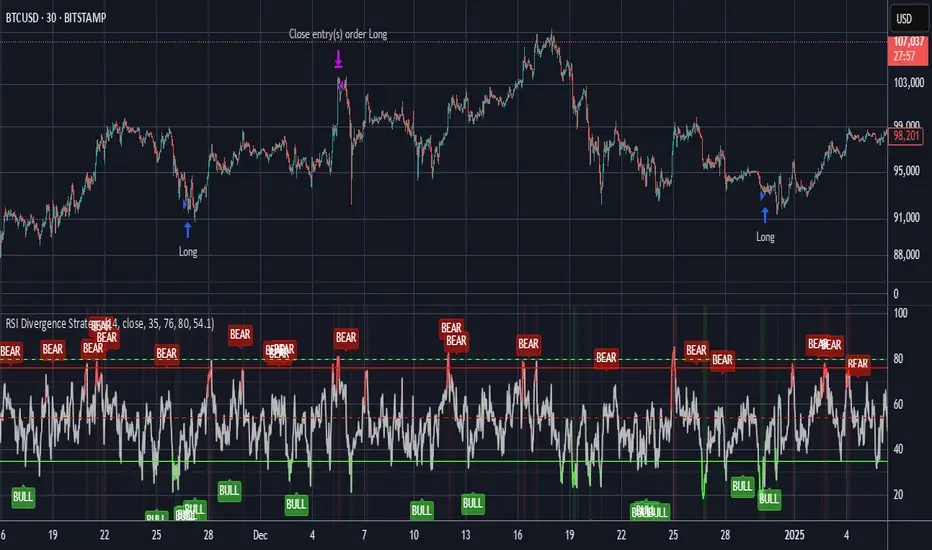
RSI Divergence StrategyOverview
The RSI Divergence Strategy Indicator is a trading tool that uses the RSI and divergences created to generate high-probability buy and sell signals.
I have provided the best formula of numbers to use for BTC on a 30 minute timeframe.
You can change where on RSI you enter and exit both long or short trades. This way you can experiment on different tokens using different entry/exit points. Can use on multiple timeframes.
This strategy is designed to open and close long or short trades based on the levels you provide it. You can then check on the RSI where the best levels are for each token you want to trade and amend it as required to generate a profitable strategy.
How It Works
The RSI Divergence Strategy Indicator uses bear and bull divergences in conjuction with a level you have input on the RSI.
RSI for Overbought/Oversold:
• Input variables for entry and exit levels and when the entry levels combine with a bear or bull divergence signal, a trade is alerted.
RSI Divergence:
• Buy and sell signals are confirmed when the RSI creates bearish or bullish divergences and these divergences are in the same area as your levels you input for entry to short or long.
After 7 years of experience and testing I have calculated the exact numbers required and produced a formula to calculate the exact input variables for a 30 minute Bitcoin chart.
Key Features
1️⃣ Divergence Identification – Ensures trades are taken only when a bull or bear divergence has formed.
2️⃣ Overbought/Oversold Input Filtering – Set up your own variables on the RSI for different markets after identifying patterns on the RSI in relation to a bearish or bullish divergence.
3️⃣ Works on any chart – Suitable for all markets and timeframes once you input the correct variables for entry and exit levels.
How to Use
🟢 Basic Trading:
• Use on any timeframe.
• Enter trade only when alert has fired off. Close when it says to exit.
• Change entry and exit levels in the properties of the strategy indicator.
• Make entry and exit levels coincide with bearish or bullish divergences on the RSI.
Check the strategy tester to see backtesting so you know if the indicator is profitable or not for that market and timeframe as each crypto token is different and so is the timeframe you choose.
📢 Webhook Automation:
• Set up TradingView Alerts to auto-execute trades via Webhook-compatible platforms.
Key additions for divergence visualization:
Divergence Arrows:
Bullish divergence: Green label with white 'bull ' text
Bearish divergence: Red label with white 'bear' text
Positioned at the pivot point
Divergence Lines:
Connects consecutive RSI pivot points
Automatically drawn between consecutive pivot points
Enhanced RSI Coloring:
Overbought zone: Red
Oversold zone: Green
Neutral zone: Gray
The visualization helps you instantly spot:
Where divergences are forming on the RSI
The pattern of higher lows (bullish) or lower highs (bearish)
Contextual coloring of RSI relative to standard levels
All divergence markers appear at the correct historical pivot points, making it easy to visually confirm divergence patterns as they develop.
Strategy levels and background zones also shown to help visual look.
Why This Combination?
This indicator is just a simple RSI tool.
It is designed to filter out weak trades and only execute trades that have:
✅ RSI Divergence
✅ Overbought or Oversold Conditions
It does not calculate downtrends or bear markets so care is recommended taking long trades during these times.
Why It’s Worth Using?
📈 Open Source – Free to use and learn from.
📉 Long or Short Term Trading Style – Entry/Exit parameters options are designed for both short or long term trades allowing you to experiment until you find a profitable strategy for that market you want to trade.
📢 Seamless Webhook Automation – Execute trades automatically with TradingView alerts.
💲 Ready to trade smarter?
✅ Add the RSI Divergence Strategy Indicator to your TradingView chart.
Strategi Pine Script®