Sentiment Bias Gauge📌 Overview
The Sentiment Bias Gauge (SBG) is a unique overlay-style indicator that visually maps a sentiment value—such as market bullishness or bearishness—onto your price chart. It converts sentiment data (in this case, RSI-based) into a floating line that moves between defined price zones, allowing users to quickly understand the current market mood in the context of price.
⚙️ How It Works
• The indicator uses RSI (Relative Strength Index) as a proxy for market sentiment (0 to 100 scale).
• This sentiment value is then mapped to a vertical price range on your chart using a configurable zone (via top and bottom percent of chart range).
• The line floats up or down within the price chart, reflecting how bullish or bearish the sentiment is.
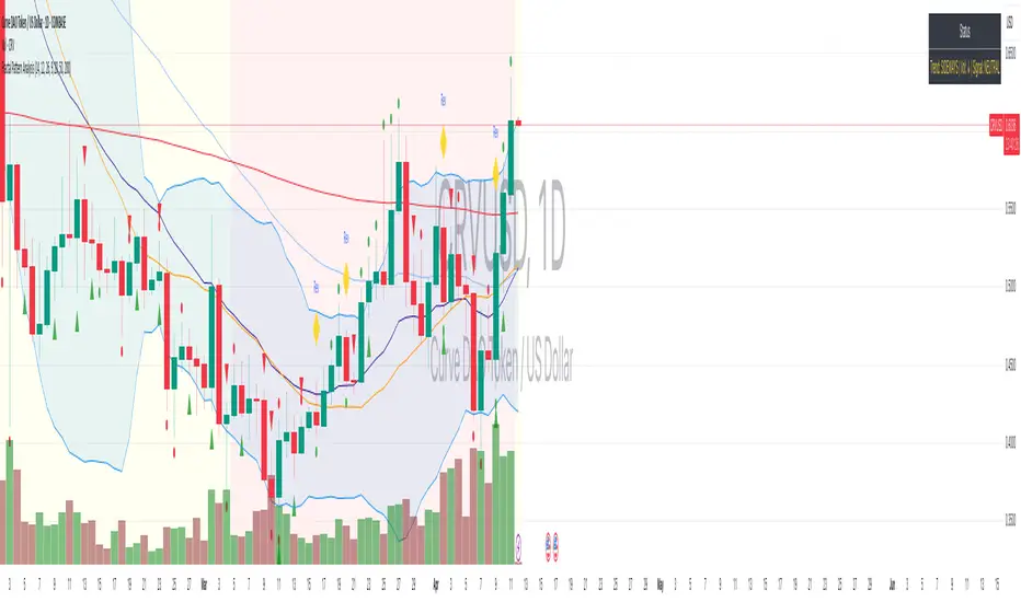
• It includes background shading to represent the sentiment level:
• 🔴 Red (Bearish): sentiment < 30
• 🟡 Yellow (Neutral): 30 ≤ sentiment ≤ 70
• 🟢 Green (Bullish): sentiment > 70
• A floating label shows the current sentiment score.
🌟 Key Features
• 📈 Overlay-Based Sentiment Line: Plots sentiment as a price-level line, giving intuitive spatial reference.
• 🔧 Configurable Range Placement: Adjust where the sentiment line appears within the chart’s high-low range.
• 🖌️ Color-Coded Background: Visually distinguish bullish, bearish, and neutral conditions.
• 🏷️ Real-Time Sentiment Label: Displays updated sentiment score on the most recent bar.
🧠 How to Use
• Use this indicator alongside your price action or technical strategy to gauge market mood.
• Combine with other sentiment indicators (e.g., fear/greed, delta volume, news sentiment).
• Especially helpful in sideways markets to identify potential shifts in bias before price reacts.
Why This Combination?
• RSI offers a reliable and intuitive proxy for market sentiment.
• Mapping the value directly onto the chart helps avoid constantly looking at a separate panel.
• The customizable chart range lets traders fit sentiment visuals within any market structure.
🎯 Why It’s Worth Using
• Makes sentiment visually accessible directly on the chart.
• Helps detect bullish/bearish bias shifts earlier than traditional indicators.
• A great tool for sentiment-aware discretionary trading or contextual overlays in algo strategies.
Penunjuk Pine Script®