TGS By ShadTGS Levels — Tesla–W.D. Gann Strategy
TGS Levels is a price-geometry indicator designed to map algorithmic decision zones on the chart using principles inspired by W.D. Gann price geometry and Tesla 3-6-9 harmonic structure.
This indicator is not a signal generator.
It provides a structured price map to help traders understand where reactions or breakouts are statistically more likely to occur.
🔹 Core Concept
Markets do not move randomly.
They rotate and expand around harmonic price cycles.
TGS Levels automatically plots a 100-unit price cycle framework (ideal for XAUUSD / Gold) and divides each cycle into hierarchical angles used by institutional and algorithmic trading models.
🔹 Level Hierarchy (Very Important)
TGS uses four types of levels, each with a different purpose:
🔴 SUPER ANGLE (+45)
Primary decision level
Price often shows strong rejection or explosive breakout
Highest importance level
🟥 MAIN ANGLES (+27, +63, +81)
High-probability reaction zones
Used for structured pullbacks, rejections, or continuation confirmation
🟠 SECONDARY ANGLES (+18, +36, +54, +72, +90)
Context & management levels
Expect hesitation, partial profit zones, or stop-tightening areas
Not recommended for direct entries
🟡 MICRO LEVELS (+3, +6, +9)
Liquidity & compression map
Help visualize absorption, stop hunts, and consolidation
For structure awareness only
🔹 What This Indicator Is Used For
✔ Identifying where price is likely to react
✔ Understanding market structure and rotation
✔ Distinguishing rejection vs breakout zones
✔ Improving trade timing when combined with:
Volatility (ATR)
Market structure (HL / LH / BOS)
Session timing (London / New York)
🔹 What This Indicator Is NOT
❌ Not a buy/sell signal
❌ Not a prediction tool
❌ Not based on indicators like RSI or MACD
TGS Levels is a price-first framework, designed to be used with price action, volatility, and structure.
🔹 Best Use Case
Asset: XAUUSD (Gold)
Execution Timeframe: M5
Sessions: London & New York
Style: Scalping / Intraday structure trading
The same logic can be adapted to other instruments by adjusting the cycle size.
🔹 How to Trade With TGS (High-Level)
When volatility is low or falling → expect rejections at main/super angles
When volatility is expanding → expect breakouts through angles
Use oscillators (like Stochastic) only for timing, not direction
Always confirm with price behavior at the level
🔹 Final Note
TGS Levels provides a clean, non-repainting price map that stays aligned when zooming or scrolling the chart.
All levels are calculated automatically and update dynamically with price.
Levels explain behavior — reactions create opportunity.
Cari dalam skrip untuk "harmonic"

TGS By ShadTGS Levels — Tesla–W.D. Gann Strategy
TGS Levels is a price-geometry indicator designed to map algorithmic decision zones on the chart using principles inspired by W.D. Gann price geometry and Tesla 3-6-9 harmonic structure.
This indicator is not a signal generator.
It provides a structured price map to help traders understand where reactions or breakouts are statistically more likely to occur.
🔹 Core Concept
Markets do not move randomly.
They rotate and expand around harmonic price cycles.
TGS Levels automatically plots a 100-unit price cycle framework (ideal for XAUUSD / Gold) and divides each cycle into hierarchical angles used by institutional and algorithmic trading models.
🔹 Level Hierarchy (Very Important)
TGS uses four types of levels, each with a different purpose:
🔴 SUPER ANGLE (+45)
Primary decision level
Price often shows strong rejection or explosive breakout
Highest importance level
🟥 MAIN ANGLES (+27, +63, +81)
High-probability reaction zones
Used for structured pullbacks, rejections, or continuation confirmation
🟠 SECONDARY ANGLES (+18, +36, +54, +72, +90)
Context & management levels
Expect hesitation, partial profit zones, or stop-tightening areas
Not recommended for direct entries
🟡 MICRO LEVELS (+3, +6, +9)
Liquidity & compression map
Help visualize absorption, stop hunts, and consolidation
For structure awareness only
🔹 What This Indicator Is Used For
✔ Identifying where price is likely to react
✔ Understanding market structure and rotation
✔ Distinguishing rejection vs breakout zones
✔ Improving trade timing when combined with:
Volatility (ATR)
Market structure (HL / LH / BOS)
Session timing (London / New York)
🔹 What This Indicator Is NOT
❌ Not a buy/sell signal
❌ Not a prediction tool
❌ Not based on indicators like RSI or MACD
TGS Levels is a price-first framework, designed to be used with price action, volatility, and structure.
🔹 Best Use Case
Asset: XAUUSD (Gold)
Execution Timeframe: M5
Sessions: London & New York
Style: Scalping / Intraday structure trading
The same logic can be adapted to other instruments by adjusting the cycle size.
🔹 How to Trade With TGS (High-Level)
When volatility is low or falling → expect rejections at main/super angles
When volatility is expanding → expect breakouts through angles
Use oscillators (like Stochastic) only for timing, not direction
Always confirm with price behavior at the level
🔹 Final Note
TGS Levels provides a clean, non-repainting price map that stays aligned when zooming or scrolling the chart.
All levels are calculated automatically and update dynamically with price.
Levels explain behavior — reactions create opportunity.

TGS by Shad TGS Levels — Tesla–W.D. Gann Strategy
TGS Levels is a price-geometry indicator designed to map algorithmic decision zones on the chart using principles inspired by W.D. Gann price geometry and Tesla 3-6-9 harmonic structure.
This indicator is not a signal generator.
It provides a structured price map to help traders understand where reactions or breakouts are statistically more likely to occur.
🔹 Core Concept
Markets do not move randomly.
They rotate and expand around harmonic price cycles.
TGS Levels automatically plots a 100-unit price cycle framework (ideal for XAUUSD / Gold) and divides each cycle into hierarchical angles used by institutional and algorithmic trading models.
🔹 Level Hierarchy (Very Important)
TGS uses four types of levels, each with a different purpose:
🔴 SUPER ANGLE (+45)
Primary decision level
Price often shows strong rejection or explosive breakout
Highest importance level
🟥 MAIN ANGLES (+27, +63, +81)
High-probability reaction zones
Used for structured pullbacks, rejections, or continuation confirmation
🟠 SECONDARY ANGLES (+18, +36, +54, +72, +90)
Context & management levels
Expect hesitation, partial profit zones, or stop-tightening areas
Not recommended for direct entries
🟡 MICRO LEVELS (+3, +6, +9)
Liquidity & compression map
Help visualize absorption, stop hunts, and consolidation
For structure awareness only
🔹 What This Indicator Is Used For
✔ Identifying where price is likely to react
✔ Understanding market structure and rotation
✔ Distinguishing rejection vs breakout zones
✔ Improving trade timing when combined with:
Volatility (ATR)
Market structure (HL / LH / BOS)
Session timing (London / New York)
🔹 What This Indicator Is NOT
❌ Not a buy/sell signal
❌ Not a prediction tool
❌ Not based on indicators like RSI or MACD
TGS Levels is a price-first framework, designed to be used with price action, volatility, and structure.
🔹 Best Use Case
Asset: XAUUSD (Gold)
Execution Timeframe: M5
Sessions: London & New York
Style: Scalping / Intraday structure trading
The same logic can be adapted to other instruments by adjusting the cycle size.
🔹 How to Trade With TGS (High-Level)
When volatility is low or falling → expect rejections at main/super angles
When volatility is expanding → expect breakouts through angles
Use oscillators (like Stochastic) only for timing, not direction
Always confirm with price behavior at the level
🔹 Final Note
TGS Levels provides a clean, non-repainting price map that stays aligned when zooming or scrolling the chart.
All levels are calculated automatically and update dynamically with price.
Levels explain behavior — reactions create opportunity.

Tesla 3-6-9 Vortex OscillatorTesla 3-6-9 Vortex Oscillator — Description
The Tesla 3-6-9 Vortex Oscillator is a unique market-structure indicator inspired by Nikola Tesla’s 3-6-9 theory, vortex mathematics, and digital-root numerical cycles.
This tool analyzes price and volume through digit-reduction patterns to track the frequency of “sacred” 3-6-9 values versus traditional 1-2-4-5-7-8 “material world” values.
Core Concept
In vortex math, all numbers reduce to a single digit (1–9).
However, 3, 6, and 9 form a special control triad, representing cyclical creation, harmony, and completion.
This indicator measures how often market data resolves into these higher-cycle digits — creating a real-time “vortex energy ratio” for trend bias and momentum shifts.
What the Indicator Measures
✔ Digital Root of Price / Volume / Range
✔ 3-6-9 Frequency vs. Counter Digit Frequency
✔ Vortex Ratio (%) – percentage dominance of 3/6/9 activity
✔ Smoothed Vortex Oscillator – trend-ready version
✔ Tesla Wave – a cyclical sine-wave based on vortex length & chosen (3, 6, or 9) multiplier
✔ Optional Visual Layers:
• Digital-root analysis
• Vortex spiral visualization
• Harmonic 3-6-9 levels
How to Use It
High Vortex Values (above 60%)
→ Market dominated by 3-6-9 cycles
→ Often aligns with expansion, breakouts, or trend strengthening
Low Vortex Values (below 40%)
→ Counter-digit dominance
→ Consolidation, weakening trend, or potential mean-reversion
Tesla Wave Crosses
→ Can signal timing windows and rhythm shifts within the cycle.
Who This Indicator Is For
• Traders who like numerical cycle analysis
• Users of vortex math, digital-root, or harmonic structures
• People who want a non-lagging sentiment oscillator
• Anyone blending TA + number theory for timing large moves

Hellenic EMA Matrix - PremiumHellenic EMA Matrix - Alpha Omega Premium
Complete User Guide
Table of Contents
Introduction
Indicator Philosophy
Mathematical Constants
EMA Types
Settings
Trading Signals
Visualization
Usage Strategies
FAQ
Introduction
Hellenic EMA Matrix is a premium indicator based on mathematical constants of nature: Phi (Phi - Golden Ratio), Pi (Pi), e (Euler's number). The indicator uses these universal constants to create dynamic EMAs that adapt to the natural rhythms of the market.
Key Features:
6 EMA types based on mathematical constants
Premium visualization with Neon Glow and Gradient Clouds
Automatic Fast/Mid/Slow EMA sorting
STRONG signals for powerful trends
Pulsing Ribbon Bar for instant trend assessment
Works on all timeframes (M1 - MN)
Indicator Philosophy
Why Mathematical Constants?
Traditional EMAs use arbitrary periods (9, 21, 50, 200). Hellenic Matrix goes further, using universal mathematical constants found in nature:
Phi (1.618) - Golden Ratio: galaxy spirals, seashells, human body proportions
Pi (3.14159) - Pi: circles, waves, cycles
e (2.71828) - Natural logarithm base: exponential growth, radioactive decay
Markets are also a natural system composed of millions of participants. Using mathematical constants allows tuning into the natural rhythms of market cycles.
Mathematical Constants
Phi (Phi) - Golden Ratio
Phi = 1.618033988749895
Properties:
Phi² = Phi + 1 = 2.618
Phi³ = 4.236
Phi⁴ = 6.854
Application: Ideal for trending movements and Fibonacci corrections
Pi (Pi) - Pi Number
Pi = 3.141592653589793
Properties:
2Pi = 6.283 (full circle)
3Pi = 9.425
4Pi = 12.566
Application: Excellent for cyclical markets and wave structures
e (Euler) - Euler's Number
e = 2.718281828459045
Properties:
e² = 7.389
e³ = 20.085
e⁴ = 54.598
Application: Suitable for exponential movements and volatile markets
EMA Types
1. Phi (Phi) - Golden Ratio EMA
Description: EMA based on the golden ratio
Period Formula:
Period = Phi^n × Base Multiplier
Parameters:
Phi Power Level (1-8): Power of Phi
Phi¹ = 1.618 → ~16 period (with Base=10)
Phi² = 2.618 → ~26 period
Phi³ = 4.236 → ~42 period (recommended)
Phi⁴ = 6.854 → ~69 period
Recommendations:
Phi² or Phi³ for day trading
Phi⁴ or Phi⁵ for swing trading
Works excellently as Fast EMA
2. Pi (Pi) - Circular EMA
Description: EMA based on Pi for cyclical movements
Period Formula:
Period = Pi × Multiple × Base Multiplier
Parameters:
Pi Multiple (1-10): Pi multiplier
1Pi = 3.14 → ~31 period (with Base=10)
2Pi = 6.28 → ~63 period (recommended)
3Pi = 9.42 → ~94 period
Recommendations:
2Pi ideal as Mid or Slow EMA
Excellently identifies cycles and waves
Use on volatile markets (crypto, forex)
3. e (Euler) - Natural EMA
Description: EMA based on natural logarithm
Period Formula:
Period = e^n × Base Multiplier
Parameters:
e Power Level (1-6): Power of e
e¹ = 2.718 → ~27 period (with Base=10)
e² = 7.389 → ~74 period (recommended)
e³ = 20.085 → ~201 period
Recommendations:
e² works excellently as Slow EMA
Ideal for stocks and indices
Filters noise well on lower timeframes
4. Delta (Delta) - Adaptive EMA
Description: Adaptive EMA that changes period based on volatility
Period Formula:
Period = Base Period × (1 + (Volatility - 1) × Factor)
Parameters:
Delta Base Period (5-200): Base period (default 20)
Delta Volatility Sensitivity (0.5-5.0): Volatility sensitivity (default 2.0)
How it works:
During low volatility → period decreases → EMA reacts faster
During high volatility → period increases → EMA smooths noise
Recommendations:
Works excellently on news and sharp movements
Use as Fast EMA for quick adaptation
Sensitivity 2.0-3.0 for crypto, 1.0-2.0 for stocks
5. Sigma (Sigma) - Composite EMA
Description: Composite EMA combining multiple active EMAs
Composition Methods:
Weighted Average (default):
Sigma = (Phi + Pi + e + Delta) / 4
Simple average of all active EMAs
Geometric Mean:
Sigma = fourth_root(Phi × Pi × e × Delta)
Geometric mean (more conservative)
Harmonic Mean:
Sigma = 4 / (1/Phi + 1/Pi + 1/e + 1/Delta)
Harmonic mean (more weight to smaller values)
Recommendations:
Enable for additional confirmation
Use as Mid EMA
Weighted Average - most universal method
6. Lambda (Lambda) - Wave EMA
Description: Wave EMA with sinusoidal period modulation
Period Formula:
Period = Base Period × (1 + Amplitude × sin(2Pi × bar / Frequency))
Parameters:
Lambda Base Period (10-200): Base period
Lambda Wave Amplitude (0.1-2.0): Wave amplitude
Lambda Wave Frequency (10-200): Wave frequency in bars
How it works:
Period pulsates sinusoidally
Creates wave effect following market cycles
Recommendations:
Experimental EMA for advanced users
Works well on cyclical markets
Frequency = 50 for day trading, 100+ for swing
Settings
Matrix Core Settings
Base Multiplier (1-100)
Multiplies all EMA periods
Base = 1: Very fast EMAs (Phi³ = 4, 2Pi = 6, e² = 7)
Base = 10: Standard (Phi³ = 42, 2Pi = 63, e² = 74)
Base = 20: Slow EMAs (Phi³ = 85, 2Pi = 126, e² = 148)
Recommendations by timeframe:
M1-M5: Base = 5-10
M15-H1: Base = 10-15 (recommended)
H4-D1: Base = 15-25
W1-MN: Base = 25-50
Matrix Source
Data source selection for EMA calculation:
close - closing price (standard)
open - opening price
high - high
low - low
hl2 - (high + low) / 2
hlc3 - (high + low + close) / 3
ohlc4 - (open + high + low + close) / 4
When to change:
hlc3 or ohlc4 for smoother signals
high for aggressive longs
low for aggressive shorts
Manual EMA Selection
Critically important setting! Determines which EMAs are used for signal generation.
Use Manual Fast/Slow/Mid Selection
Enabled (default): You select EMAs manually
Disabled: Automatic selection by periods
Fast EMA
Fast EMA - reacts first to price changes
Recommendations:
Phi Golden (recommended) - universal choice
Delta Adaptive - for volatile markets
Must be fastest (smallest period)
Slow EMA
Slow EMA - determines main trend
Recommendations:
Pi Circular (recommended) - excellent trend filter
e Natural - for smoother trend
Must be slowest (largest period)
Mid EMA
Mid EMA - additional signal filter
Recommendations:
e Natural (recommended) - excellent middle level
Pi Circular - alternative
None - for more frequent signals (only 2 EMAs)
IMPORTANT: The indicator automatically sorts selected EMAs by their actual periods:
Fast = EMA with smallest period
Mid = EMA with middle period
Slow = EMA with largest period
Therefore, you can select any combination - the indicator will arrange them correctly!
Premium Visualization
Neon Glow
Enable Neon Glow for EMAs - adds glowing effect around EMA lines
Glow Strength:
Light - subtle glow
Medium (recommended) - optimal balance
Strong - bright glow (may be too bright)
Effect: 2 glow layers around each EMA for 3D effect
Gradient Clouds
Enable Gradient Clouds - fills space between EMAs with gradient
Parameters:
Cloud Transparency (85-98): Cloud transparency
95-97 (recommended)
Higher = more transparent
Dynamic Cloud Intensity - automatically changes transparency based on EMA distance
Cloud Colors:
Phi-Pi Cloud:
Blue - when Pi above Phi (bullish)
Gold - when Phi above Pi (bearish)
Pi-e Cloud:
Green - when e above Pi (bullish)
Blue - when Pi above e (bearish)
2 layers for volumetric effect
Pulsing Ribbon Bar
Enable Pulsing Indicator Bar - pulsing strip at bottom/top of chart
Parameters:
Ribbon Position: Top / Bottom (recommended)
Pulse Speed: Slow / Medium (recommended) / Fast
Symbols and colors:
Green filled square - STRONG BULLISH
Pink filled square - STRONG BEARISH
Blue hollow square - Bullish (regular)
Red hollow square - Bearish (regular)
Purple rectangle - Neutral
Effect: Pulsation with sinusoid for living market feel
Signal Bar Highlights
Enable Signal Bar Highlights - highlights bars with signals
Parameters:
Highlight Transparency (88-96): Highlight transparency
Highlight Style:
Light Fill (recommended) - bar background fill
Thin Line - bar outline only
Highlights:
Golden Cross - green
Death Cross - pink
STRONG BUY - green
STRONG SELL - pink
Show Greek Labels
Shows Greek alphabet letters on last bar:
Phi - Phi EMA (gold)
Pi - Pi EMA (blue)
e - Euler EMA (green)
Delta - Delta EMA (purple)
Sigma - Sigma EMA (pink)
When to use: For education or presentations
Show Old Background
Old background style (not recommended):
Green background - STRONG BULLISH
Pink background - STRONG BEARISH
Blue background - Bullish
Red background - Bearish
Not recommended - use new Gradient Clouds and Pulsing Bar
Info Table
Show Info Table - table with indicator information
Parameters:
Position: Top Left / Top Right (recommended) / Bottom Left / Bottom Right
Size: Tiny / Small (recommended) / Normal / Large
Table contents:
EMA list - periods and current values of all active EMAs
Effects - active visual effects
TREND - current trend state:
STRONG UP - strong bullish
STRONG DOWN - strong bearish
Bullish - regular bullish
Bearish - regular bearish
Neutral - neutral
Momentum % - percentage deviation of price from Fast EMA
Setup - current Fast/Slow/Mid configuration
Trading Signals
Show Golden/Death Cross
Golden Cross - Fast EMA crosses Slow EMA from below (bullish signal) Death Cross - Fast EMA crosses Slow EMA from above (bearish signal)
Symbols:
Yellow dot "GC" below - Golden Cross
Dark red dot "DC" above - Death Cross
Show STRONG Signals
STRONG BUY and STRONG SELL - the most powerful indicator signals
Conditions for STRONG BULLISH:
EMA Alignment: Fast > Mid > Slow (all EMAs aligned)
Trend: Fast > Slow (clear uptrend)
Distance: EMAs separated by minimum 0.15%
Price Position: Price above Fast EMA
Fast Slope: Fast EMA rising
Slow Slope: Slow EMA rising
Mid Trending: Mid EMA also rising (if enabled)
Conditions for STRONG BEARISH:
Same but in reverse
Visual display:
Green label "STRONG BUY" below bar
Pink label "STRONG SELL" above bar
Difference from Golden/Death Cross:
Golden/Death Cross = crossing moment (1 bar)
STRONG signal = sustained trend (lasts several bars)
IMPORTANT: After fixes, STRONG signals now:
Work on all timeframes (M1 to MN)
Don't break on small retracements
Work with any Fast/Mid/Slow combination
Automatically adapt thanks to EMA sorting
Show Stop Loss/Take Profit
Automatic SL/TP level calculation on STRONG signal
Parameters:
Stop Loss (ATR) (0.5-5.0): ATR multiplier for stop loss
1.5 (recommended) - standard
1.0 - tight stop
2.0-3.0 - wide stop
Take Profit R:R (1.0-5.0): Risk/reward ratio
2.0 (recommended) - standard (risk 1.5 ATR, profit 3.0 ATR)
1.5 - conservative
3.0-5.0 - aggressive
Formulas:
LONG:
Stop Loss = Entry - (ATR × Stop Loss ATR)
Take Profit = Entry + (ATR × Stop Loss ATR × Take Profit R:R)
SHORT:
Stop Loss = Entry + (ATR × Stop Loss ATR)
Take Profit = Entry - (ATR × Stop Loss ATR × Take Profit R:R)
Visualization:
Red X - Stop Loss
Green X - Take Profit
Levels remain active while STRONG signal persists
Trading Signals
Signal Types
1. Golden Cross
Description: Fast EMA crosses Slow EMA from below
Signal: Beginning of bullish trend
How to trade:
ENTRY: On bar close with Golden Cross
STOP: Below local low or below Slow EMA
TARGET: Next resistance level or 2:1 R:R
Strengths:
Simple and clear
Works well on trending markets
Clear entry point
Weaknesses:
Lags (signal after movement starts)
Many false signals in ranging markets
May be late on fast moves
Optimal timeframes: H1, H4, D1
2. Death Cross
Description: Fast EMA crosses Slow EMA from above
Signal: Beginning of bearish trend
How to trade:
ENTRY: On bar close with Death Cross
STOP: Above local high or above Slow EMA
TARGET: Next support level or 2:1 R:R
Application: Mirror of Golden Cross
3. STRONG BUY
Description: All EMAs aligned + trend + all EMAs rising
Signal: Powerful bullish trend
How to trade:
ENTRY: On bar close with STRONG BUY or on pullback to Fast EMA
STOP: Below Fast EMA or automatic SL (if enabled)
TARGET: Automatic TP (if enabled) or by levels
TRAILING: Follow Fast EMA
Entry strategies:
Aggressive: Enter immediately on signal
Conservative: Wait for pullback to Fast EMA, then enter on bounce
Pyramiding: Add positions on pullbacks to Mid EMA
Position management:
Hold while STRONG signal active
Exit on STRONG SELL or Death Cross appearance
Move stop behind Fast EMA
Strengths:
Most reliable indicator signal
Doesn't break on pullbacks
Catches large moves
Works on all timeframes
Weaknesses:
Appears less frequently than other signals
Requires confirmation (multiple conditions)
Optimal timeframes: All (M5 - D1)
4. STRONG SELL
Description: All EMAs aligned down + downtrend + all EMAs falling
Signal: Powerful bearish trend
How to trade: Mirror of STRONG BUY
Visual Signals
Pulsing Ribbon Bar
Quick market assessment at a glance:
Symbol Color State
Filled square Green STRONG BULLISH
Filled square Pink STRONG BEARISH
Hollow square Blue Bullish
Hollow square Red Bearish
Rectangle Purple Neutral
Pulsation: Sinusoidal, creates living effect
Signal Bar Highlights
Bars with signals are highlighted:
Green highlight: STRONG BUY or Golden Cross
Pink highlight: STRONG SELL or Death Cross
Gradient Clouds
Colored space between EMAs shows trend strength:
Wide clouds - strong trend
Narrow clouds - weak trend or consolidation
Color change - trend change
Info Table
Quick reference in corner:
TREND: Current state (STRONG UP, Bullish, Neutral, Bearish, STRONG DOWN)
Momentum %: Movement strength
Effects: Active visual effects
Setup: Fast/Slow/Mid configuration
Usage Strategies
Strategy 1: "Golden Trailing"
Idea: Follow STRONG signals using Fast EMA as trailing stop
Settings:
Fast: Phi Golden (Phi³)
Mid: Pi Circular (2Pi)
Slow: e Natural (e²)
Base Multiplier: 10
Timeframe: H1, H4
Entry rules:
Wait for STRONG BUY
Enter on bar close or on pullback to Fast EMA
Stop below Fast EMA
Management:
Hold position while STRONG signal active
Move stop behind Fast EMA daily
Exit on STRONG SELL or Death Cross
Take Profit:
Partially close at +2R
Trail remainder until exit signal
For whom: Swing traders, trend followers
Pros:
Catches large moves
Simple rules
Emotionally comfortable
Cons:
Requires patience
Possible extended drawdowns on pullbacks
Strategy 2: "Scalping Bounces"
Idea: Scalp bounces from Fast EMA during STRONG trend
Settings:
Fast: Delta Adaptive (Base 15, Sensitivity 2.0)
Mid: Phi Golden (Phi²)
Slow: Pi Circular (2Pi)
Base Multiplier: 5
Timeframe: M5, M15
Entry rules:
STRONG signal must be active
Wait for price pullback to Fast EMA
Enter on bounce (candle closes above/below Fast EMA)
Stop behind local extreme (15-20 pips)
Take Profit:
+1.5R or to Mid EMA
Or to next level
For whom: Active day traders
Pros:
Many signals
Clear entry point
Quick profits
Cons:
Requires constant monitoring
Not all bounces work
Requires discipline for frequent trading
Strategy 3: "Triple Filter"
Idea: Enter only when all 3 EMAs and price perfectly aligned
Settings:
Fast: Phi Golden (Phi³)
Mid: e Natural (e²)
Slow: Pi Circular (3Pi)
Base Multiplier: 15
Timeframe: H4, D1
Entry rules (LONG):
STRONG BUY active
Price above all three EMAs
Fast > Mid > Slow (all aligned)
All EMAs rising (slope up)
Gradient Clouds wide and bright
Entry:
On bar close meeting all conditions
Or on next pullback to Fast EMA
Stop:
Below Mid EMA or -1.5 ATR
Take Profit:
First target: +3R
Second target: next major level
Trailing: Mid EMA
For whom: Conservative swing traders, investors
Pros:
Very reliable signals
Minimum false entries
Large profit potential
Cons:
Rare signals (2-5 per month)
Requires patience
Strategy 4: "Adaptive Scalper"
Idea: Use only Delta Adaptive EMA for quick volatility reaction
Settings:
Fast: Delta Adaptive (Base 10, Sensitivity 3.0)
Mid: None
Slow: Delta Adaptive (Base 30, Sensitivity 2.0)
Base Multiplier: 3
Timeframe: M1, M5
Feature: Two different Delta EMAs with different settings
Entry rules:
Golden Cross between two Delta EMAs
Both Delta EMAs must be rising/falling
Enter on next bar
Stop:
10-15 pips or below Slow Delta EMA
Take Profit:
+1R to +2R
Or Death Cross
For whom: Scalpers on cryptocurrencies and forex
Pros:
Instant volatility adaptation
Many signals on volatile markets
Quick results
Cons:
Much noise on calm markets
Requires fast execution
High commissions may eat profits
Strategy 5: "Cyclical Trader"
Idea: Use Pi and Lambda for trading cyclical markets
Settings:
Fast: Pi Circular (1Pi)
Mid: Lambda Wave (Base 30, Amplitude 0.5, Frequency 50)
Slow: Pi Circular (3Pi)
Base Multiplier: 10
Timeframe: H1, H4
Entry rules:
STRONG signal active
Lambda Wave EMA synchronized with trend
Enter on bounce from Lambda Wave
For whom: Traders of cyclical assets (some altcoins, commodities)
Pros:
Catches cyclical movements
Lambda Wave provides additional entry points
Cons:
More complex to configure
Not for all markets
Lambda Wave may give false signals
Strategy 6: "Multi-Timeframe Confirmation"
Idea: Use multiple timeframes for confirmation
Scheme:
Higher TF (D1): Determine trend direction (STRONG signal)
Middle TF (H4): Wait for STRONG signal in same direction
Lower TF (M15): Look for entry point (Golden Cross or bounce from Fast EMA)
Settings for all TFs:
Fast: Phi Golden (Phi³)
Mid: e Natural (e²)
Slow: Pi Circular (2Pi)
Base Multiplier: 10
Rules:
All 3 TFs must show one trend
Entry on lower TF
Stop by lower TF
Target by higher TF
For whom: Serious traders and investors
Pros:
Maximum reliability
Large profit targets
Minimum false signals
Cons:
Rare setups
Requires analysis of multiple charts
Experience needed
Practical Tips
DOs
Use STRONG signals as primary - they're most reliable
Let signals develop - don't exit on first pullback
Use trailing stop - follow Fast EMA
Combine with levels - S/R, Fibonacci, volumes
Test on demo before real
Adjust Base Multiplier for your timeframe
Enable visual effects - they help see the picture
Use Info Table - quick situation assessment
Watch Pulsing Bar - instant state indicator
Trust auto-sorting of Fast/Mid/Slow
DON'Ts
Don't trade against STRONG signal - trend is your friend
Don't ignore Mid EMA - it adds reliability
Don't use too small Base Multiplier on higher TFs
Don't enter on Golden Cross in range - check for trend
Don't change settings during open position
Don't forget risk management - 1-2% per trade
Don't trade all signals in row - choose best ones
Don't use indicator in isolation - combine with Price Action
Don't set too tight stops - let trade breathe
Don't over-optimize - simplicity = reliability
Optimal Settings by Asset
US Stocks (SPY, AAPL, TSLA)
Recommendation:
Fast: Phi Golden (Phi³)
Mid: e Natural (e²)
Slow: Pi Circular (2Pi)
Base: 10-15
Timeframe: H4, D1
Features:
Use on daily for swing
STRONG signals very reliable
Works well on trending stocks
Forex (EUR/USD, GBP/USD)
Recommendation:
Fast: Delta Adaptive (Base 15, Sens 2.0)
Mid: Phi Golden (Phi²)
Slow: Pi Circular (2Pi)
Base: 8-12
Timeframe: M15, H1, H4
Features:
Delta Adaptive works excellently on news
Many signals on M15-H1
Consider spreads
Cryptocurrencies (BTC, ETH, altcoins)
Recommendation:
Fast: Delta Adaptive (Base 10, Sens 3.0)
Mid: Pi Circular (2Pi)
Slow: e Natural (e²)
Base: 5-10
Timeframe: M5, M15, H1
Features:
High volatility - adaptation needed
STRONG signals can last days
Be careful with scalping on M1-M5
Commodities (Gold, Oil)
Recommendation:
Fast: Pi Circular (1Pi)
Mid: Phi Golden (Phi³)
Slow: Pi Circular (3Pi)
Base: 12-18
Timeframe: H4, D1
Features:
Pi works excellently on cyclical commodities
Gold responds especially well to Phi
Oil volatile - use wide stops
Indices (S&P500, Nasdaq, DAX)
Recommendation:
Fast: Phi Golden (Phi³)
Mid: e Natural (e²)
Slow: Pi Circular (2Pi)
Base: 15-20
Timeframe: H4, D1, W1
Features:
Very trending instruments
STRONG signals last weeks
Good for position trading
Alerts
The indicator supports 6 alert types:
1. Golden Cross
Message: "Hellenic Matrix: GOLDEN CROSS - Fast EMA crossed above Slow EMA - Bullish trend starting!"
When: Fast EMA crosses Slow EMA from below
2. Death Cross
Message: "Hellenic Matrix: DEATH CROSS - Fast EMA crossed below Slow EMA - Bearish trend starting!"
When: Fast EMA crosses Slow EMA from above
3. STRONG BULLISH
Message: "Hellenic Matrix: STRONG BULLISH SIGNAL - All EMAs aligned for powerful uptrend!"
When: All conditions for STRONG BUY met (first bar)
4. STRONG BEARISH
Message: "Hellenic Matrix: STRONG BEARISH SIGNAL - All EMAs aligned for powerful downtrend!"
When: All conditions for STRONG SELL met (first bar)
5. Bullish Ribbon
Message: "Hellenic Matrix: BULLISH RIBBON - EMAs aligned for uptrend"
When: EMAs aligned bullish + price above Fast EMA (less strict condition)
6. Bearish Ribbon
Message: "Hellenic Matrix: BEARISH RIBBON - EMAs aligned for downtrend"
When: EMAs aligned bearish + price below Fast EMA (less strict condition)
How to Set Up Alerts:
Open indicator on chart
Click on three dots next to indicator name
Select "Create Alert"
In "Condition" field select needed alert:
Golden Cross
Death Cross
STRONG BULLISH
STRONG BEARISH
Bullish Ribbon
Bearish Ribbon
Configure notification method:
Pop-up in browser
Email
SMS (in Premium accounts)
Push notifications in mobile app
Webhook (for automation)
Select frequency:
Once Per Bar Close (recommended) - once on bar close
Once Per Bar - during bar formation
Only Once - only first time
Click "Create"
Tip: Create separate alerts for different timeframes and instruments
FAQ
1. Why don't STRONG signals appear?
Possible reasons:
Incorrect Fast/Mid/Slow order
Solution: Indicator automatically sorts EMAs by periods, but ensure selected EMAs have different periods
Base Multiplier too large
Solution: Reduce Base to 5-10 on lower timeframes
Market in range
Solution: STRONG signals appear only in trends - this is normal
Too strict EMA settings
Solution: Try classic combination: Phi³ / Pi×2 / e² with Base=10
Mid EMA too close to Fast or Slow
Solution: Select Mid EMA with period between Fast and Slow
2. How often should STRONG signals appear?
Normal frequency:
M1-M5: 5-15 signals per day (very active markets)
M15-H1: 2-8 signals per day
H4: 3-10 signals per week
D1: 2-5 signals per month
W1: 2-6 signals per year
If too many signals - market very volatile or Base too small
If too few signals - market in range or Base too large
4. What are the best settings for beginners?
Universal "out of the box" settings:
Matrix Core:
Base Multiplier: 10
Source: close
Phi Golden: Enabled, Power = 3
Pi Circular: Enabled, Multiple = 2
e Natural: Enabled, Power = 2
Delta Adaptive: Enabled, Base = 20, Sensitivity = 2.0
Manual Selection:
Fast: Phi Golden
Mid: e Natural
Slow: Pi Circular
Visualization:
Gradient Clouds: ON
Neon Glow: ON (Medium)
Pulsing Bar: ON (Medium)
Signal Highlights: ON (Light Fill)
Table: ON (Top Right, Small)
Signals:
Golden/Death Cross: ON
STRONG Signals: ON
Stop Loss: OFF (while learning)
Timeframe for learning: H1 or H4
5. Can I use only one EMA?
No, minimum 2 EMAs (Fast and Slow) for signal generation.
Mid EMA is optional:
With Mid EMA = more reliable but rarer signals
Without Mid EMA = more signals but less strict filtering
Recommendation: Start with 3 EMAs (Fast/Mid/Slow), then experiment
6. Does the indicator work on cryptocurrencies?
Yes, works excellently! Especially good on:
Bitcoin (BTC)
Ethereum (ETH)
Major altcoins (SOL, BNB, XRP)
Recommended settings for crypto:
Fast: Delta Adaptive (Base 10-15, Sensitivity 2.5-3.0)
Mid: Pi Circular (2Pi)
Slow: e Natural (e²)
Base: 5-10
Timeframe: M15, H1, H4
Crypto market features:
High volatility → use Delta Adaptive
24/7 trading → set alerts
Sharp movements → wide stops
7. Can I trade only with this indicator?
Technically yes, but NOT recommended.
Best approach - combine with:
Price Action - support/resistance levels, candle patterns
Volume - movement strength confirmation
Fibonacci - retracement and extension levels
RSI/MACD - divergences and overbought/oversold
Fundamental analysis - news, company reports
Hellenic Matrix:
Excellently determines trend and its strength
Provides clear entry/exit points
Doesn't consider fundamentals
Doesn't see major levels
8. Why do Gradient Clouds change color?
Color depends on EMA order:
Phi-Pi Cloud:
Blue - Pi EMA above Phi EMA (bullish alignment)
Gold - Phi EMA above Pi EMA (bearish alignment)
Pi-e Cloud:
Green - e EMA above Pi EMA (bullish alignment)
Blue - Pi EMA above e EMA (bearish alignment)
Color change = EMA order change = possible trend change
9. What is Momentum % in the table?
Momentum % = percentage deviation of price from Fast EMA
Formula:
Momentum = ((Close - Fast EMA) / Fast EMA) × 100
Interpretation:
+0.5% to +2% - normal bullish momentum
+2% to +5% - strong bullish momentum
+5% and above - overheating (correction possible)
-0.5% to -2% - normal bearish momentum
-2% to -5% - strong bearish momentum
-5% and below - oversold (bounce possible)
Usage:
Monitor momentum during STRONG signals
Large momentum = don't enter (wait for pullback)
Small momentum = good entry point
10. How to configure for scalping?
Settings for scalping (M1-M5):
Base Multiplier: 3-5
Source: close or hlc3 (smoother)
Fast: Delta Adaptive (Base 8-12, Sensitivity 3.0)
Mid: None (for more signals)
Slow: Phi Golden (Phi²) or Pi Circular (1Pi)
Visualization:
- Gradient Clouds: ON (helps see strength)
- Neon Glow: OFF (doesn't clutter chart)
- Pulsing Bar: ON (quick assessment)
- Signal Highlights: ON
Signals:
- Golden/Death Cross: ON
- STRONG Signals: ON
- Stop Loss: ON (1.0-1.5 ATR, R:R 1.5-2.0)
Scalping rules:
Trade only STRONG signals
Enter on bounce from Fast EMA
Tight stops (10-20 pips)
Quick take profit (+1R to +2R)
Don't hold through news
11. How to configure for long-term investing?
Settings for investing (D1-W1):
Base Multiplier: 20-30
Source: close
Fast: Phi Golden (Phi³ or Phi⁴)
Mid: e Natural (e²)
Slow: Pi Circular (3Pi or 4Pi)
Visualization:
- Gradient Clouds: ON
- Neon Glow: ON (Medium)
- Everything else - to taste
Signals:
- Golden/Death Cross: ON
- STRONG Signals: ON
- Stop Loss: OFF (use percentage stop)
Investing rules:
Enter only on STRONG signals
Hold while STRONG active (weeks/months)
Stop below Slow EMA or -10%
Take profit: by company targets or +50-100%
Ignore short-term pullbacks
12. What if indicator slows down chart?
Indicator is optimized, but if it slows:
Disable unnecessary visual effects:
Neon Glow: OFF (saves 8 plots)
Gradient Clouds: ON but low quality
Lambda Wave EMA: OFF (if not using)
Reduce number of active EMAs:
Sigma Composite: OFF
Lambda Wave: OFF
Leave only Phi, Pi, e, Delta
Simplify settings:
Pulsing Bar: OFF
Greek Labels: OFF
Info Table: smaller size
13. Can I use on different timeframes simultaneously?
Yes! Multi-timeframe analysis is very powerful:
Classic scheme:
Higher TF (D1, W1) - determine global trend
Wait for STRONG signal
This is our trading direction
Middle TF (H4, H1) - look for confirmation
STRONG signal in same direction
Precise entry zone
Lower TF (M15, M5) - entry point
Golden Cross or bounce from Fast EMA
Precise stop loss
Example:
W1: STRONG BUY active (global uptrend)
H4: STRONG BUY appeared (confirmation)
M15: Wait for Golden Cross or bounce from Fast EMA → ENTRY
Advantages:
Maximum reliability
Clear timeframe hierarchy
Large targets
14. How does indicator work on news?
Delta Adaptive EMA adapts excellently to news:
Before news:
Low volatility → Delta EMA becomes fast → pulls to price
During news:
Sharp volatility spike → Delta EMA slows → filters noise
After news:
Volatility normalizes → Delta EMA returns to normal
Recommendations:
Don't trade at news release moment (spreads widen)
Wait for STRONG signal after news (2-5 bars)
Use Delta Adaptive as Fast EMA for quick reaction
Widen stops by 50-100% during important news
Advanced Techniques
Technique 1: "Divergences with EMA"
Idea: Look for discrepancies between price and Fast EMA
Bullish divergence:
Price makes lower low
Fast EMA makes higher low
= Possible reversal up
Bearish divergence:
Price makes higher high
Fast EMA makes lower high
= Possible reversal down
How to trade:
Find divergence
Wait for STRONG signal in divergence direction
Enter on confirmation
Technique 2: "EMA Tunnel"
Idea: Use space between Fast and Slow EMA as "tunnel"
Rules:
Wide tunnel - strong trend, hold position
Narrow tunnel - weak trend or consolidation, caution
Tunnel narrowing - trend weakening, prepare to exit
Tunnel widening - trend strengthening, can add
Visually: Gradient Clouds show this automatically!
Trading:
Enter on STRONG signal (tunnel starts widening)
Hold while tunnel wide
Exit when tunnel starts narrowing
Technique 3: "Wave Analysis with Lambda"
Idea: Lambda Wave EMA creates sinusoid matching market cycles
Setup:
Lambda Base Period: 30
Lambda Wave Amplitude: 0.5
Lambda Wave Frequency: 50 (adjusted to asset cycle)
How to find correct Frequency:
Look at historical cycles (distance between local highs)
Average distance = your Frequency
Example: if highs every 40-60 bars, set Frequency = 50
Trading:
Enter when Lambda Wave at bottom of sinusoid (growth potential)
Exit when Lambda Wave at top (fall potential)
Combine with STRONG signals
Technique 4: "Cluster Analysis"
Idea: When all EMAs gather in narrow cluster = powerful breakout soon
Cluster signs:
All EMAs (Phi, Pi, e, Delta) within 0.5-1% of each other
Gradient Clouds almost invisible
Price jumping around all EMAs
Trading:
Identify cluster (all EMAs close)
Determine breakout direction (where more volume, higher TFs direction)
Wait for breakout and STRONG signal
Enter on confirmation
Target = cluster size × 3-5
This is very powerful technique for big moves!
Technique 5: "Sigma as Dynamic Level"
Idea: Sigma Composite EMA = average of all EMAs = magnetic level
Usage:
Enable Sigma Composite (Weighted Average)
Sigma works as dynamic support/resistance
Price often returns to Sigma before trend continuation
Trading:
In trend: Enter on bounces from Sigma
In range: Fade moves from Sigma (trade return to Sigma)
On breakout: Sigma becomes support/resistance
Risk Management
Basic Rules
1. Position Size
Conservative: 1% of capital per trade
Moderate: 2% of capital per trade (recommended)
Aggressive: 3-5% (only for experienced)
Calculation formula:
Lot Size = (Capital × Risk%) / (Stop in pips × Pip value)
2. Risk/Reward Ratio
Minimum: 1:1.5
Standard: 1:2 (recommended)
Optimal: 1:3
Aggressive: 1:5+
3. Maximum Drawdown
Daily: -3% to -5%
Weekly: -7% to -10%
Monthly: -15% to -20%
Upon reaching limit → STOP trading until end of period
Position Management Strategies
1. Fixed Stop
Method:
Stop below/above Fast EMA or local extreme
DON'T move stop against position
Can move to breakeven
For whom: Beginners, conservative traders
2. Trailing by Fast EMA
Method:
Each day (or bar) move stop to Fast EMA level
Position closes when price breaks Fast EMA
Advantages:
Stay in trend as long as possible
Automatically exit on reversal
For whom: Trend followers, swing traders
3. Partial Exit
Method:
50% of position close at +2R
50% hold with trailing by Mid EMA or Slow EMA
Advantages:
Lock profit
Leave position for big move
Psychologically comfortable
For whom: Universal method (recommended)
4. Pyramiding
Method:
First entry on STRONG signal (50% of planned position)
Add 25% on pullback to Fast EMA
Add another 25% on pullback to Mid EMA
Overall stop below Slow EMA
Advantages:
Average entry price
Reduce risk
Increase profit in strong trends
Caution:
Works only in trends
In range leads to losses
For whom: Experienced traders
Trading Psychology
Correct Mindset
1. Indicator is a tool, not holy grail
Indicator shows probability, not guarantee
There will be losing trades - this is normal
Important is series statistics, not one trade
2. Trust the system
If STRONG signal appeared - enter
Don't search for "perfect" moment
Follow trading plan
3. Patience
STRONG signals don't appear every day
Better miss signal than enter against trend
Quality over quantity
4. Discipline
Always set stop loss
Don't move stop against position
Don't increase risk after losses
Beginner Mistakes
1. "I know better than indicator"
Indicator says STRONG BUY, but you think "too high, will wait for pullback"
Result: miss profitable move
Solution: Trust signals or don't use indicator
2. "Will reverse now for sure"
Trading against STRONG trend
Result: stops, stops, stops
Solution: Trend is your friend, trade with trend
3. "Will hold a bit more"
Don't exit when STRONG signal disappears
Greed eats profit
Solution: If signal gone - exit!
4. "I'll recover"
After losses double risk
Result: huge losses
Solution: Fixed % risk ALWAYS
5. "I don't like this signal"
Skip signals because of "feeling"
Result: inconsistency, no statistics
Solution: Trade ALL signals or clearly define filters
Trading Journal
What to Record
For each trade:
1. Entry/exit date and time
2. Instrument and timeframe
3. Signal type
Golden Cross
STRONG BUY
STRONG SELL
Death Cross
4. Indicator settings
Fast/Mid/Slow EMA
Base Multiplier
Other parameters
5. Chart screenshot
Entry moment
Exit moment
6. Trade parameters
Position size
Stop loss
Take Profit
R:R
7. Result
Profit/Loss in $
Profit/Loss in %
Profit/Loss in R
8. Notes
What was right
What was wrong
Emotions during trade
Lessons
Journal Analysis
Analyze weekly:
1. Win Rate
Win Rate = (Profitable trades / All trades) × 100%
Good: 50-60%
Excellent: 60-70%
Exceptional: 70%+
2. Average R
Average R = Sum of all R / Number of trades
Good: +0.5R
Excellent: +1.0R
Exceptional: +1.5R+
3. Profit Factor
Profit Factor = Total profit / Total losses
Good: 1.5+
Excellent: 2.0+
Exceptional: 3.0+
4. Maximum Drawdown
Track consecutive losses
If more than 5 in row - stop, check system
5. Best/Worst Trades
What was common in best trades? (do more)
What was common in worst trades? (avoid)
Pre-Trade Checklist
Technical Analysis
STRONG signal active (BUY or SELL)
All EMAs properly aligned (Fast > Mid > Slow or reverse)
Price on correct side of Fast EMA
Gradient Clouds confirm trend
Pulsing Bar shows STRONG state
Momentum % in normal range (not overheated)
No close strong levels against direction
Higher timeframe doesn't contradict
Risk Management
Position size calculated (1-2% risk)
Stop loss set
Take profit calculated (minimum 1:2)
R:R satisfactory
Daily/weekly risk limit not exceeded
No other open correlated positions
Fundamental Analysis
No important news in coming hours
Market session appropriate (liquidity)
No contradicting fundamentals
Understand why asset is moving
Psychology
Calm and thinking clearly
No emotions from previous trades
Ready to accept loss at stop
Following trading plan
Not revenging market for past losses
If at least one point is NO - think twice before entering!
Learning Roadmap
Week 1: Familiarization
Goals:
Install and configure indicator
Study all EMA types
Understand visualization
Tasks:
Add indicator to chart
Test all Fast/Mid/Slow settings
Play with Base Multiplier on different timeframes
Observe Gradient Clouds and Pulsing Bar
Study Info Table
Result: Comfort with indicator interface
Week 2: Signals
Goals:
Learn to recognize all signal types
Understand difference between Golden Cross and STRONG
Tasks:
Find 10 Golden Cross examples in history
Find 10 STRONG BUY examples in history
Compare their results (which worked better)
Set up alerts
Get 5 real alerts
Result: Understanding signals
Week 3: Demo Trading
Goals:
Start trading signals on demo account
Gather statistics
Tasks:
Open demo account
Trade ONLY STRONG signals
Keep journal (minimum 20 trades)
Don't change indicator settings
Strictly follow stop losses
Result: 20+ documented trades
Week 4: Analysis
Goals:
Analyze demo trading results
Optimize approach
Tasks:
Calculate win rate and average R
Find patterns in profitable trades
Find patterns in losing trades
Adjust approach (not indicator!)
Write trading plan
Result: Trading plan on 1 page
Month 2: Improvement
Goals:
Deepen understanding
Add additional techniques
Tasks:
Study multi-timeframe analysis
Test combinations with Price Action
Try advanced techniques (divergences, tunnels)
Continue demo trading (minimum 50 trades)
Achieve stable profitability on demo
Result: Win rate 55%+ and Profit Factor 1.5+
Month 3: Real Trading
Goals:
Transition to real account
Maintain discipline
Tasks:
Open small real account
Trade minimum lots
Strictly follow trading plan
DON'T increase risk
Focus on process, not profit
Result: Psychological comfort on real
Month 4+: Scaling
Goals:
Increase account
Become consistently profitable
Tasks:
With 60%+ win rate can increase risk to 2%
Upon doubling account can add capital
Continue keeping journal
Periodically review and improve strategy
Share experience with community
Result: Stable profitability month after month
Additional Resources
Recommended Reading
Technical Analysis:
"Technical Analysis of Financial Markets" - John Murphy
"Trading in the Zone" - Mark Douglas (psychology)
"Market Wizards" - Jack Schwager (trader interviews)
EMA and Moving Averages:
"Moving Averages 101" - Steve Burns
Articles on Investopedia about EMA
Risk Management:
"The Mathematics of Money Management" - Ralph Vince
"Trade Your Way to Financial Freedom" - Van K. Tharp
Trading Journals:
Edgewonk (paid, very powerful)
Tradervue (free version + premium)
Excel/Google Sheets (free)
Screeners:
TradingView Stock Screener
Finviz (stocks)
CoinMarketCap (crypto)
Conclusion
Hellenic EMA Matrix is a powerful tool based on universal mathematical constants of nature. The indicator combines:
Mathematical elegance - Phi, Pi, e instead of arbitrary numbers
Premium visualization - Neon Glow, Gradient Clouds, Pulsing Bar
Reliable signals - STRONG BUY/SELL work on all timeframes
Flexibility - 6 EMA types, adaptation to any trading style
Automation - auto-sorting EMAs, SL/TP calculation, alerts
Key Success Principles:
Simplicity - start with basic settings (Phi/Pi/e, Base=10)
Discipline - follow STRONG signals strictly
Patience - wait for quality setups
Risk Management - 1-2% per trade, ALWAYS
Journal - document every trade
Learning - constantly improve skills
Remember:
Indicator shows probability, not guarantee
Important is series statistics, not one trade
Psychology more important than technique
Quality more important than quantity
Process more important than result
Acknowledgments
Thank you for using Hellenic EMA Matrix - Alpha Omega Premium!
The indicator was created with love for mathematics, markets, and beautiful visualization.
Wishing you profitable trading!
Guide Version: 1.0
Date: 2025
Compatibility: Pine Script v6, TradingView
"In the simplicity of mathematical constants lies the complexity of market movements"

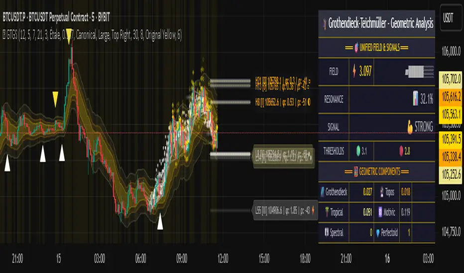
Grothendieck-Teichmüller Geometric SynthesisDskyz's Grothendieck-Teichmüller Geometric Synthesis (GTGS)
THEORETICAL FOUNDATION: A SYMPHONY OF GEOMETRIES
The 🎓 GTGS is built upon a revolutionary premise: that market dynamics can be modeled as geometric and topological structures. While not a literal academic implementation—such a task would demand computational power far beyond current trading platforms—it leverages core ideas from advanced mathematical theories as powerful analogies and frameworks for its algorithms. Each component translates an abstract concept into a practical market calculation, distinguishing GTGS by identifying deeper structural patterns rather than relying on standard statistical measures.
1. Grothendieck-Teichmüller Theory: Deforming Market Structure
The Theory : Studies symmetries and deformations of geometric objects, focusing on the "absolute" structure of mathematical spaces.
Indicator Analogy : The calculate_grothendieck_field function models price action as a "deformation" from its immediate state. Using the nth root of price ratios (math.pow(price_ratio, 1.0/prime)), it measures market "shape" stretching or compression, revealing underlying tensions and potential shifts.
2. Topos Theory & Sheaf Cohomology: From Local to Global Patterns
The Theory : A framework for assembling local properties into a global picture, with cohomology measuring "obstructions" to consistency.
Indicator Analogy : The calculate_topos_coherence function uses sine waves (math.sin) to represent local price "sections." Summing these yields a "cohomology" value, quantifying price action consistency. High values indicate coherent trends; low values signal conflict and uncertainty.
3. Tropical Geometry: Simplifying Complexity
The Theory : Transforms complex multiplicative problems into simpler, additive, piecewise-linear ones using min(a, b) for addition and a + b for multiplication.
Indicator Analogy : The calculate_tropical_metric function applies tropical_add(a, b) => math.min(a, b) to identify the "lowest energy" state among recent price points, pinpointing critical support levels non-linearly.
4. Motivic Cohomology & Non-Commutative Geometry
The Theory : Studies deep arithmetic and quantum-like properties of geometric spaces.
Indicator Analogy : The motivic_rank and spectral_triple functions compute weighted sums of historical prices to capture market "arithmetic complexity" and "spectral signature." Higher values reflect structured, harmonic price movements.
5. Perfectoid Spaces & Homotopy Type Theory
The Theory : Abstract fields dealing with p-adic numbers and logical foundations of mathematics.
Indicator Analogy : The perfectoid_conv and type_coherence functions analyze price convergence and path identity, assessing the "fractal dust" of price differences and price path cohesion, adding fractal and logical analysis.
The Combination is Key : No single theory dominates. GTGS ’s Unified Field synthesizes all seven perspectives into a comprehensive score, ensuring signals reflect deep structural alignment across mathematical domains.
🎛️ INPUTS: CONFIGURING THE GEOMETRIC ENGINE
The GTGS offers a suite of customizable inputs, allowing traders to tailor its behavior to specific timeframes, market sectors, and trading styles. Below is a detailed breakdown of key input groups, their functionality, and optimization strategies, leveraging provided tooltips for precision.
Grothendieck-Teichmüller Theory Inputs
🧬 Deformation Depth (Absolute Galois) :
What It Is : Controls the depth of Galois group deformations analyzed in market structure.
How It Works : Measures price action deformations under automorphisms of the absolute Galois group, capturing market symmetries.
Optimization :
Higher Values (15-20) : Captures deeper symmetries, ideal for major trends in swing trading (4H-1D).
Lower Values (3-8) : Responsive to local deformations, suited for scalping (1-5min).
Timeframes :
Scalping (1-5min) : 3-6 for quick local shifts.
Day Trading (15min-1H) : 8-12 for balanced analysis.
Swing Trading (4H-1D) : 12-20 for deep structural trends.
Sectors :
Stocks : Use 8-12 for stable trends.
Crypto : 3-8 for volatile, short-term moves.
Forex : 12-15 for smooth, cyclical patterns.
Pro Tip : Increase in trending markets to filter noise; decrease in choppy markets for sensitivity.
🗼 Teichmüller Tower Height :
What It Is : Determines the height of the Teichmüller modular tower for hierarchical pattern detection.
How It Works : Builds modular levels to identify nested market patterns.
Optimization :
Higher Values (6-8) : Detects complex fractals, ideal for swing trading.
Lower Values (2-4) : Focuses on primary patterns, faster for scalping.
Timeframes :
Scalping : 2-3 for speed.
Day Trading : 4-5 for balanced patterns.
Swing Trading : 5-8 for deep fractals.
Sectors :
Indices : 5-8 for robust, long-term patterns.
Crypto : 2-4 for rapid shifts.
Commodities : 4-6 for cyclical trends.
Pro Tip : Higher towers reveal hidden fractals but may slow computation; adjust based on hardware.
🔢 Galois Prime Base :
What It Is : Sets the prime base for Galois field computations.
How It Works : Defines the field extension characteristic for market analysis.
Optimization :
Prime Characteristics :
2 : Binary markets (up/down).
3 : Ternary states (bull/bear/neutral).
5 : Pentagonal symmetry (Elliott waves).
7 : Heptagonal cycles (weekly patterns).
11,13,17,19 : Higher-order patterns.
Timeframes :
Scalping/Day Trading : 2 or 3 for simplicity.
Swing Trading : 5 or 7 for wave or cycle detection.
Sectors :
Forex : 5 for Elliott wave alignment.
Stocks : 7 for weekly cycle consistency.
Crypto : 3 for volatile state shifts.
Pro Tip : Use 7 for most markets; 5 for Elliott wave traders.
Topos Theory & Sheaf Cohomology Inputs
🏛️ Temporal Site Size :
What It Is : Defines the number of time points in the topological site.
How It Works : Sets the local neighborhood for sheaf computations, affecting cohomology smoothness.
Optimization :
Higher Values (30-50) : Smoother cohomology, better for trends in swing trading.
Lower Values (5-15) : Responsive, ideal for reversals in scalping.
Timeframes :
Scalping : 5-10 for quick responses.
Day Trading : 15-25 for balanced analysis.
Swing Trading : 25-50 for smooth trends.
Sectors :
Stocks : 25-35 for stable trends.
Crypto : 5-15 for volatility.
Forex : 20-30 for smooth cycles.
Pro Tip : Match site size to your average holding period in bars for optimal coherence.
📐 Sheaf Cohomology Degree :
What It Is : Sets the maximum degree of cohomology groups computed.
How It Works : Higher degrees capture complex topological obstructions.
Optimization :
Degree Meanings :
1 : Simple obstructions (basic support/resistance).
2 : Cohomological pairs (double tops/bottoms).
3 : Triple intersections (complex patterns).
4-5 : Higher-order structures (rare events).
Timeframes :
Scalping/Day Trading : 1-2 for simplicity.
Swing Trading : 3 for complex patterns.
Sectors :
Indices : 2-3 for robust patterns.
Crypto : 1-2 for rapid shifts.
Commodities : 3-4 for cyclical events.
Pro Tip : Degree 3 is optimal for most trading; higher degrees for research or rare event detection.
🌐 Grothendieck Topology :
What It Is : Chooses the Grothendieck topology for the site.
How It Works : Affects how local data integrates into global patterns.
Optimization :
Topology Characteristics :
Étale : Finest topology, captures local-global principles.
Nisnevich : A1-invariant, good for trends.
Zariski : Coarse but robust, filters noise.
Fpqc : Faithfully flat, highly sensitive.
Sectors :
Stocks : Zariski for stability.
Crypto : Étale for sensitivity.
Forex : Nisnevich for smooth trends.
Indices : Zariski for robustness.
Timeframes :
Scalping : Étale for precision.
Swing Trading : Nisnevich or Zariski for reliability.
Pro Tip : Start with Étale for precision; switch to Zariski in noisy markets.
Unified Field Configuration Inputs
⚛️ Field Coupling Constant :
What It Is : Sets the interaction strength between geometric components.
How It Works : Controls signal amplification in the unified field equation.
Optimization :
Higher Values (0.5-1.0) : Strong coupling, amplified signals for ranging markets.
Lower Values (0.001-0.1) : Subtle signals for trending markets.
Timeframes :
Scalping : 0.5-0.8 for quick, strong signals.
Swing Trading : 0.1-0.3 for trend confirmation.
Sectors :
Crypto : 0.5-1.0 for volatility.
Stocks : 0.1-0.3 for stability.
Forex : 0.3-0.5 for balance.
Pro Tip : Default 0.137 (fine structure constant) is a balanced starting point; adjust up in choppy markets.
📐 Geometric Weighting Scheme :
What It Is : Determines the framework for combining geometric components.
How It Works : Adjusts emphasis on different mathematical structures.
Optimization :
Scheme Characteristics :
Canonical : Equal weighting, balanced.
Derived : Emphasizes higher-order structures.
Motivic : Prioritizes arithmetic properties.
Spectral : Focuses on frequency domain.
Sectors :
Stocks : Canonical for balance.
Crypto : Spectral for volatility.
Forex : Derived for structured moves.
Indices : Motivic for arithmetic cycles.
Timeframes :
Day Trading : Canonical or Derived for flexibility.
Swing Trading : Motivic for long-term cycles.
Pro Tip : Start with Canonical; experiment with Spectral in volatile markets.
Dashboard and Visual Configuration Inputs
📋 Show Enhanced Dashboard, 📏 Size, 📍 Position :
What They Are : Control dashboard visibility, size, and placement.
How They Work : Display key metrics like Unified Field , Resonance , and Signal Quality .
Optimization :
Scalping : Small size, Bottom Right for minimal chart obstruction.
Swing Trading : Large size, Top Right for detailed analysis.
Sectors : Universal across markets; adjust size based on screen setup.
Pro Tip : Use Large for analysis, Small for live trading.
📐 Show Motivic Cohomology Bands, 🌊 Morphism Flow, 🔮 Future Projection, 🔷 Holographic Mesh, ⚛️ Spectral Flow :
What They Are : Toggle visual elements representing mathematical calculations.
How They Work : Provide intuitive representations of market dynamics.
Optimization :
Timeframes :
Scalping : Enable Morphism Flow and Spectral Flow for momentum.
Swing Trading : Enable all for comprehensive analysis.
Sectors :
Crypto : Emphasize Morphism Flow and Future Projection for volatility.
Stocks : Focus on Cohomology Bands for stable trends.
Pro Tip : Disable non-essential visuals in fast markets to reduce clutter.
🌫️ Field Transparency, 🔄 Web Recursion Depth, 🎨 Mesh Color Scheme :
What They Are : Adjust visual clarity, complexity, and color.
How They Work : Enhance interpretability of visual elements.
Optimization :
Transparency : 30-50 for balanced visibility; lower for analysis.
Recursion Depth : 6-8 for balanced detail; lower for older hardware.
Color Scheme :
Purple/Blue : Analytical focus.
Green/Orange : Trading momentum.
Pro Tip : Use Neon Purple for deep analysis; Neon Green for active trading.
⏱️ Minimum Bars Between Signals :
What It Is : Minimum number of bars required between consecutive signals.
How It Works : Prevents signal clustering by enforcing a cooldown period.
Optimization :
Higher Values (10-20) : Fewer signals, avoids whipsaws, suited for swing trading.
Lower Values (0-5) : More responsive, allows quick reversals, ideal for scalping.
Timeframes :
Scalping : 0-2 bars for rapid signals.
Day Trading : 3-5 bars for balance.
Swing Trading : 5-10 bars for stability.
Sectors :
Crypto : 0-3 for volatility.
Stocks : 5-10 for trend clarity.
Forex : 3-7 for cyclical moves.
Pro Tip : Increase in choppy markets to filter noise.
Hardcoded Parameters
Tropical, Motivic, Spectral, Perfectoid, Homotopy Inputs : Fixed to optimize performance but influence calculations (e.g., tropical_degree=4 for support levels, perfectoid_prime=5 for convergence).
Optimization : Experiment with codebase modifications if advanced customization is needed, but defaults are robust across markets.
🎨 ADVANCED VISUAL SYSTEM: TRADING IN A GEOMETRIC UNIVERSE
The GTTMTSF ’s visuals are direct representations of its mathematics, designed for intuitive and precise trading decisions.
Motivic Cohomology Bands :
What They Are : Dynamic bands ( H⁰ , H¹ , H² ) representing cohomological support/resistance.
Color & Meaning : Colors reflect energy levels ( H⁰ tightest, H² widest). Breaks into H¹ signal momentum; H² touches suggest reversals.
How to Trade : Use for stop-loss/profit-taking. Band bounces with Dashboard confirmation are high-probability setups.
Morphism Flow (Webbing) :
What It Is : White particle streams visualizing market momentum.
Interpretation : Dense flows indicate strong trends; sparse flows signal consolidation.
How to Trade : Follow dominant flow direction; new flows post-consolidation signal trend starts.
Future Projection Web (Fractal Grid) :
What It Is : Fibonacci-period fractal projections of support/resistance.
Color & Meaning : Three-layer lines (white shadow, glow, colored quantum) with labels showing price, topological class, anomaly strength (φ), resonance (ρ), and obstruction ( H¹ ). ⚡ marks extreme anomalies.
How to Trade : Target ⚡/● levels for entries/exits. High-anomaly levels with weakening Unified Field are reversal setups.
Holographic Mesh & Spectral Flow :
What They Are : Visuals of harmonic interference and spectral energy.
How to Trade : Bright mesh nodes or strong Spectral Flow warn of building pressure before price movement.
📊 THE GEOMETRIC DASHBOARD: YOUR MISSION CONTROL
The Dashboard translates complex mathematics into actionable intelligence.
Unified Field & Signals :
FIELD : Master value (-10 to +10), synthesizing all geometric components. Extreme readings (>5 or <-5) signal structural limits, often preceding reversals or continuations.
RESONANCE : Measures harmony between geometric field and price-volume momentum. Positive amplifies bullish moves; negative amplifies bearish moves.
SIGNAL QUALITY : Confidence meter rating alignment. Trade only STRONG or EXCEPTIONAL signals for high-probability setups.
Geometric Components :
What They Are : Breakdown of seven mathematical engines.
How to Use : Watch for convergence. A strong Unified Field is reliable when components (e.g., Grothendieck , Topos , Motivic ) align. Divergence warns of trend weakening.
Signal Performance :
What It Is : Tracks indicator signal performance.
How to Use : Assesses real-time performance to build confidence and understand system behavior.
🚀 DEVELOPMENT & UNIQUENESS: BEYOND CONVENTIONAL ANALYSIS
The GTTMTSF was developed to analyze markets as evolving geometric objects, not statistical time-series.
Why This Is Unlike Anything Else :
Theoretical Depth : Uses geometry and topology, identifying patterns invisible to statistical tools.
Holistic Synthesis : Integrates seven deep mathematical frameworks into a cohesive Unified Field .
Creative Implementation : Translates PhD-level mathematics into functional Pine Script , blending theory and practice.
Immersive Visualization : Transforms charts into dynamic geometric landscapes for intuitive market understanding.
The GTTMTSF is more than an indicator; it’s a new lens for viewing markets, for traders seeking deeper insight into hidden order within chaos.
" Where there is matter, there is geometry. " - Johannes Kepler
— Dskyz , Trade with insight. Trade with anticipation.
BK AK-Scope🔭 Introducing BK AK-Scope — Target Locked. Signal Acquired. 🔭
After building five precision weapons for traders, I’m proud to unveil the sixth.
BK AK-Scope — the eye of the arsenal.
This is not just an indicator. It’s an intelligence system for volatility, signal clarity, and rate-of-change dynamics — forged for elite vision in any market terrain.
🧠 Why “Scope”? And Why “AK”?
Every shooter knows: you can’t hit what you can’t see.
The Scope brings range, clarity, and target distinction. It filters motion from noise. Purpose from panic.
“AK” continues to honor the man who trained my sight — my mentor, A.K.
His discipline taught me to wait for alignment. To move with reason, not emotion.
His vision lives in every code line here.
🔬 What Is BK AK-Scope?
A Triple-Tier TSI Correlation Engine, fused with adaptive opacity logic, a volatility scoring system, and real-time signal clarity. It’s momentum dissected — by speed, depth, and rate of change.
Built to serve traders who:
Need visual hierarchy between fast, mid, and slow TSI responses.
Want adaptive fills that pulse with volatility — not static zones.
Require a volatility scoring overlay that reads the battlefield in real time.
⚙️ Core Systems: How BK AK-Scope Works
✅ Fast/Mid/Slow TSI →
Three layers of correlation: like scopes with zoom levels.
You track micro moves, mid swings, and macro flow simultaneously.
✅ Rate-of-Change Adaptive Opacity →
Momentum fills fade or flash based on speed — giving you movement density at a glance.
Bull vs. Bear zones adapt to strength. You feel the market’s pulse.
✅ Volatility Score Intelligence →
Custom algorithm measuring:
Range expansion
Rate-of-change differentials
ATR dynamics
Standard deviation pressure
All combined into a score from 0–100 with live icons:
🔥 = Extreme Heat (70+)
🧊 = Cold Zone (<30)
⚠️ = ROC Warning
• = Neutral drift
✅ Auto-Detect Volatility Modes →
Scalp = <15min
Swing = intraday/hourly
Macro = daily/weekly
Or override manually with total control.
🎯 How To Use BK AK-Scope
🔹 Trend Continuation → When all three TSI layers align in direction + volatility score climbs, ride with the trend.
🔹 Early Reversals → Opposing TSI + rapid opacity change + volatility shift = sniper reversal zone.
🔹 Consolidation Filter → Neutral fills + score < 30 = stay out, wait for signal surge.
🔹 Signal Confluence → Pair with:
• Gann fans or angles
• Fib time/price clusters
• Elliott Wave structure
• Harmonics or divergence
To isolate entry perfection.
🛡️ Why This Indicator Changes the Game
It's not just momentum. It’s TSI with depth hierarchy.
It’s not just color. It’s real-time strength visualization.
It’s not just volatility. It’s rate-weighted market intelligence.
This is market optics for the advanced trader — built for vision, clarity, and discipline.
🙏 Final Thoughts
🔹 In honor of A.K., my mentor. The man who taught me to see what others miss.
🔹 Inspired by the power of vision — because execution without clarity is chaos.
🔹 Powered by faith — because Gd alone gives sight beyond the visible.
“He gives sight to the blind and wisdom to the humble.” — Psalms 146
Every tool I build is a prayer in code — that it helps someone trade with clarity, integrity, and precision.
⚡ Zoom In. Focus Deep. Trade Clean.
BK AK-Scope — Lock on the target. See what others don’t.
🔫 Clarity is power. 🔫
Gd bless. 🙏

Mandelbrot-Fibonacci Cascade Vortex (MFCV)Mandelbrot-Fibonacci Cascade Vortex (MFCV) - Where Chaos Theory Meets Sacred Geometry
A Revolutionary Synthesis of Fractal Mathematics and Golden Ratio Dynamics
What began as an exploration into Benoit Mandelbrot's fractal market hypothesis and the mysterious appearance of Fibonacci sequences in nature has culminated in a groundbreaking indicator that reveals the hidden mathematical structure underlying market movements. This indicator represents months of research into chaos theory, fractal geometry, and the golden ratio's manifestation in financial markets.
The Theoretical Foundation
Mandelbrot's Fractal Market Hypothesis Traditional efficient market theory assumes normal distributions and random walks. Mandelbrot proved markets are fractal - self-similar patterns repeating across all timeframes with power-law distributions. The MFCV implements this through:
Hurst Exponent Calculation: H = log(R/S) / log(n/2)
Where:
R = Range of cumulative deviations
S = Standard deviation
n = Period length
This measures market memory:
H > 0.5: Trending (persistent) behavior
H = 0.5: Random walk
H < 0.5: Mean-reverting (anti-persistent) behavior
Fractal Dimension: D = 2 - H
This quantifies market complexity, where higher dimensions indicate more chaotic behavior.
Fibonacci Vortex Theory Markets don't move linearly - they spiral. The MFCV reveals these spirals using Fibonacci sequences:
Vortex Calculation: Vortex(n) = Price + sin(bar_index × φ / Fn) × ATR(Fn) × Volume_Factor
Where:
φ = 0.618 (golden ratio)
Fn = Fibonacci number (8, 13, 21, 34, 55)
Volume_Factor = 1 + (Volume/SMA(Volume,50) - 1) × 0.5
This creates oscillating spirals that contract and expand with market energy.
The Volatility Cascade System
Markets exhibit volatility clustering - Mandelbrot's "Noah Effect." The MFCV captures this through cascading volatility bands:
Cascade Level Calculation: Level(i) = ATR(20) × φ^i
Each level represents a different fractal scale, creating a multi-dimensional view of market structure. The golden ratio spacing ensures harmonic resonance between levels.
Implementation Architecture
Core Components:
Fractal Analysis Engine
Calculates Hurst exponent over user-defined periods
Derives fractal dimension for complexity measurement
Identifies market regime (trending/ranging/chaotic)
Fibonacci Vortex Generator
Creates 5 independent spiral oscillators
Each spiral follows a Fibonacci period
Volume amplification creates dynamic response
Cascade Band System
Up to 8 volatility levels
Golden ratio expansion between levels
Dynamic coloring based on fractal state
Confluence Detection
Identifies convergence of vortex and cascade levels
Highlights high-probability reversal zones
Real-time confluence strength calculation
Signal Generation Logic
The MFCV generates two primary signal types:
Fractal Signals: Generated when:
Hurst > 0.65 (strong trend) AND volatility expanding
Hurst < 0.35 (mean reversion) AND RSI < 35
Trend strength > 0.4 AND vortex alignment
Cascade Signals: Triggered by:
RSI > 60 AND price > SMA(50) AND bearish vortex
RSI < 40 AND price < SMA(50) AND bullish vortex
Volatility expansion AND trend strength > 0.3
Both signals implement a 15-bar cooldown to prevent overtrading.
Advanced Input System
Mandelbrot Parameters:
Cascade Levels (3-8):
Controls number of volatility bands
Crypto: 5-7 (high volatility)
Indices: 4-5 (moderate volatility)
Forex: 3-4 (low volatility)
Hurst Period (20-200):
Lookback for fractal calculation
Scalping: 20-50
Day Trading: 50-100
Swing Trading: 100-150
Position Trading: 150-200
Cascade Ratio (1.0-3.0):
Band width multiplier
1.618: Golden ratio (default)
Higher values for trending markets
Lower values for ranging markets
Fractal Memory (21-233):
Fibonacci retracement lookback
Uses Fibonacci numbers for harmonic alignment
Fibonacci Vortex Settings:
Spiral Periods:
Comma-separated Fibonacci sequence
Fast: "5,8,13,21,34" (scalping)
Standard: "8,13,21,34,55" (balanced)
Extended: "13,21,34,55,89" (swing)
Rotation Speed (0.1-2.0):
Controls spiral oscillation frequency
0.618: Golden ratio (balanced)
Higher = more signals, more noise
Lower = smoother, fewer signals
Volume Amplification:
Enables dynamic spiral expansion
Essential for stocks and crypto
Disable for forex (no central volume)
Visual System Architecture
Cascade Bands:
Multi-level volatility envelopes
Gradient coloring from primary to secondary theme
Transparency increases with distance from price
Fill between bands shows fractal structure
Vortex Spirals:
5 Fibonacci-period oscillators
Blue above price (bullish pressure)
Red below price (bearish pressure)
Multiple display styles: Lines, Circles, Dots, Cross
Dynamic Fibonacci Levels:
Auto-updating retracement levels
Smart update logic prevents disruption near levels
Distance-based transparency (closer = more visible)
Updates every 50 bars or on volatility spikes
Confluence Zones:
Highlighted boxes where indicators converge
Stronger confluence = stronger support/resistance
Key areas for reversal trades
Professional Dashboard System
Main Fractal Dashboard: Displays real-time:
Hurst Exponent with market state
Fractal Dimension with complexity level
Volatility Cascade status
Vortex rotation impact
Market regime classification
Signal strength percentage
Active indicator levels
Vortex Metrics Panel: Shows:
Individual spiral deviations
Convergence/divergence metrics
Real-time vortex positioning
Fibonacci period performance
Fractal Metrics Display: Tracks:
Dimension D value
Market complexity rating
Self-similarity strength
Trend quality assessment
Theory Guide Panel: Educational reference showing:
Mandelbrot principles
Fibonacci vortex concepts
Dynamic trading suggestions
Trading Applications
Trend Following:
High Hurst (>0.65) indicates strong trends
Follow cascade band direction
Use vortex spirals for entry timing
Exit when Hurst drops below 0.5
Mean Reversion:
Low Hurst (<0.35) signals reversal potential
Trade toward vortex spiral convergence
Use Fibonacci levels as targets
Tighten stops in chaotic regimes
Breakout Trading:
Monitor cascade band compression
Watch for vortex spiral alignment
Volatility expansion confirms breakouts
Use confluence zones for targets
Risk Management:
Position size based on fractal dimension
Wider stops in high complexity markets
Tighter stops when Hurst is extreme
Scale out at Fibonacci levels
Market-Specific Optimization
Cryptocurrency:
Cascade Levels: 5-7
Hurst Period: 50-100
Rotation Speed: 0.786-1.2
Enable volume amplification
Stock Indices:
Cascade Levels: 4-5
Hurst Period: 80-120
Rotation Speed: 0.5-0.786
Moderate cascade ratio
Forex:
Cascade Levels: 3-4
Hurst Period: 100-150
Rotation Speed: 0.382-0.618
Disable volume amplification
Commodities:
Cascade Levels: 4-6
Hurst Period: 60-100
Rotation Speed: 0.5-1.0
Seasonal adjustment consideration
Innovation and Originality
The MFCV represents several breakthrough innovations:
First Integration of Mandelbrot Fractals with Fibonacci Vortex Theory
Unique synthesis of chaos theory and sacred geometry
Novel application of Hurst exponent to spiral dynamics
Dynamic Volatility Cascade System
Golden ratio-based band expansion
Multi-timeframe fractal analysis
Self-adjusting to market conditions
Volume-Amplified Vortex Spirals
Revolutionary spiral calculation method
Dynamic response to market participation
Multiple Fibonacci period integration
Intelligent Signal Generation
Cooldown system prevents overtrading
Multi-factor confirmation required
Regime-aware signal filtering
Professional Analytics Dashboard
Institutional-grade metrics display
Real-time fractal analysis
Educational integration
Development Journey
Creating the MFCV involved overcoming numerous challenges:
Mathematical Complexity: Implementing Hurst exponent calculations efficiently
Visual Clarity: Displaying multiple indicators without cluttering
Performance Optimization: Managing array operations and calculations
Signal Quality: Balancing sensitivity with reliability
User Experience: Making complex theory accessible
The result is an indicator that brings PhD-level mathematics to practical trading while maintaining visual elegance and usability.
Best Practices and Guidelines
Start Simple: Use default settings initially
Match Timeframe: Adjust parameters to your trading style
Confirm Signals: Never trade MFCV signals in isolation
Respect Regimes: Adapt strategy to market state
Manage Risk: Use fractal dimension for position sizing
Color Themes
Six professional themes included:
Fractal: Balanced blue/purple palette
Golden: Warm Fibonacci-inspired colors
Plasma: Vibrant modern aesthetics
Cosmic: Dark mode optimized
Matrix: Classic green terminal
Fire: Heat map visualization
Disclaimer
This indicator is for educational and research purposes only. It does not constitute financial advice. While the MFCV reveals deep market structure through advanced mathematics, markets remain inherently unpredictable. Past performance does not guarantee future results.
The integration of Mandelbrot's fractal theory with Fibonacci vortex dynamics provides unique market insights, but should be used as part of a comprehensive trading strategy. Always use proper risk management and never risk more than you can afford to lose.
Acknowledgments
Special thanks to Benoit Mandelbrot for revolutionizing our understanding of markets through fractal geometry, and to the ancient mathematicians who discovered the golden ratio's universal significance.
"The geometry of nature is fractal... Markets are fractal too." - Benoit Mandelbrot
Revealing the Hidden Order in Market Chaos Trade with Mathematical Precision. Trade with MFCV.
— Created with passion for the TradingView community
Trade with insight. Trade with anticipation.
— Dskyz , for DAFE Trading Systems

Multi-Factor Reversal AnalyzerMulti-Factor Reversal Analyzer – Quantitative Reversal Signal System
OVERVIEW
Multi-Factor Reversal Analyzer is a comprehensive technical analysis toolkit designed to detect market tops and bottoms with high precision. It combines trend momentum analysis, price action behavior, wave oscillation structure, and volatility breakout potential into one unified indicator.
This indicator is not a random mix of tools — each module is carefully selected for a specific purpose. When combined, they form a multi-dimensional view of the market, merging trend analysis, momentum divergence, and volatility compression to produce high-confidence signals.
Why Combine These Modules?
Module Combination Ideas & How to Use Them
Factor A: Trend Detector + Gold Zone
Concept:
• The Trend Detector (light yellow histogram) evaluates market strength:
• Histogram trending downward or staying below 50 → bearish conditions;
• Trending upward or staying above 50 → bullish conditions.
• The Gold Zone identifies areas of volatility compression — typically a prelude to explosive market moves.
Practical Application:
• When the Gold Zone appears and the Trend Detector is bearish → likely downside move;
• When the Gold Zone appears and the Trend Detector is bullish → likely upside breakout.
• Note: The Gold Zone does not mean the bottom is in. It is not a buy signal on its own — always combine it with other modules for directional bias.
Factor B: PAI + Wave Trend
Concept:
• PAI (Price Action Index) is a custom oscillator that combines price momentum with volatility dispersion, displaying strength zones:
• Green area → bullish dominance;
• Red area → bearish pressure.
• Wave Trend offers smoothed crossover signals via the main and signal lines.
Practical Application:
• When PAI is in the green zone and Wave Trend makes a bullish crossover → potential reversal to the upside;
• When PAI is in the red zone and Wave Trend shows a bearish crossover → potential start of a downtrend.
Factor C: Trend Detector + PAI
Concept:
• Combines directional trend strength with price action strength to confirm setups via confluence.
Practical Application:
• Trend Detector histogram bottoms out + PAI enters the green zone → high chance of upward reversal;
• Histogram tops out + PAI in the red zone → increased likelihood of downside continuation.
Multi-Factor Confluence (Advanced Use)
• When Trend Detector, PAI, and Wave Trend all align in the same direction (bullish or bearish), the directional signal becomes significantly more reliable.
• This setup is especially useful for trend-following or swing trade entries.
KEY FEATURES
1. Multi-Layer Reversal Logic
• Combines trend scoring, oscillator divergence, and volatility squeezes for triangulated reversal detection.
• Helps traders distinguish between trend pullbacks and true reversals.
2. Advanced Divergence Detection
• Detects both regular and hidden divergences using pivot-based confirmation logic.
• Customizable lookback ranges and pivot sensitivity provide flexible tuning for different market styles.
3. Gold Zone Volatility Compression
• Highlights pre-breakout zones using custom oscillation models (RSI, harmonic, Karobein, etc.).
• Improves anticipation of breakout opportunities following low-volatility compressions.
4. Trend Direction Context
• PAI and Trend Score components provide top-down insight into prevailing bias.
• Built-in “Straddle Area” highlights consolidation zones; breakouts from this area often signal new trend phases.
5. Flexible Visualization
• Color-coded trend bars, reversal markers, normalized oscillator plots, and trend strength labels.
• Designed for both visual discretionary traders and data-driven system developers.
USAGE GUIDELINES
1. Applicable Markets
• Suitable for stocks, crypto, futures, and forex
• Supports reversal, mean-reversion, and breakout trading styles
2. Recommended Timeframes
• Short-term traders: 5m / 15m / 1H — use Wave Trend divergence + Gold Zone
• Swing traders: 4H / Daily — rely on Price Action Index and Trend Detector
• Macro trend context: use PAI HTF mode for higher timeframe overlays
3. Reversal Strategy Flow
• Watch for divergence (WT/PAI) + Gold Zone compression
• Confirm with Trend Score weakening or flipping
• Use Straddle Area breakout for final trigger
• Optional: enable bar coloring or labels for visual reinforcement
• The indicator performs optimally when used in conjunction with a harmonic pattern recognition tool
4. Additional Note on the Gold Zone
The “Gold Zone” does not directly indicate a market bottom. Since it is displayed at the bottom of the chart, it may be misunderstood as a bullish signal. In reality, the Gold Zone represents a compression of price momentum and volatility, suggesting that a significant directional move is about to occur. The direction of that move—upward or downward—should be determined by analyzing the histogram:
• If histogram momentum is weakening, the Gold Zone may precede a downward move.
• If histogram momentum is strengthening, it may signal an upcoming rebound or rally.
Treat the Gold Zone as a warning of impending volatility, and always combine it with trend indicators for accurate directional judgment.
RISK DISCLAIMER
• This indicator calculates trend direction based on historical data and cannot guarantee future market performance. When using this indicator for trading, always combine it with other technical analysis tools, fundamental analysis, and personal trading experience for comprehensive decision-making.
• Market conditions are uncertain, and trend signals may result in false positives or lag. Traders should avoid over-reliance on indicator signals and implement stop-loss strategies and risk management techniques to reduce potential losses.
• Leverage trading carries high risks and may result in rapid capital loss. If using this indicator in leveraged markets (such as futures, forex, or cryptocurrency derivatives), exercise caution, manage risks properly, and set reasonable stop-loss/take-profit levels to protect funds.
• All trading decisions are the sole responsibility of the trader. The developer is not liable for any trading losses. This indicator is for technical analysis reference only and does not constitute investment advice.
• Before live trading, it is recommended to use a demo account for testing to fully understand how to use the indicator and apply proper risk management strategies.
CHANGELOG
v1.0: Initial release featuring integrated Price Action Index, Trend Strength Scoring, Wave Trend Oscillator, Gold Zone Compression Detection, and dual-type divergence recognition. Supports higher timeframe (HTF) synchronization, visual signal markers, and diversified parameter configurations.

RawCuts_01Library "RawCuts_01"
A collection of functions by:
mutantdog
The majority of these are used within published projects, some useful variants have been included here aswell.
This is volume one consisting mainly of smaller functions, predominantly the filters and standard deviations from Weight Gain 4000.
Also included at the bottom are various snippets of related code for demonstration. These can be copied and adjusted according to your needs.
A full up-to-date table of contents is located at the top of the main script.
WEIGHT GAIN FILTERS
A collection of moving average type filters with adjustable volume weighting.
Based upon the two most common methods of volume weighting.
'Simple' uses the standard method in which a basic VWMA is analogous to SMA.
'Elastic' uses exponential method found in EVWMA which is analogous to RMA.
Volume weighting is applied according to an exponent multiplier of input volume.
0 >> volume^0 (unweighted), 1 >> volume^1 (fully weighted), use float values for intermediate weighting.
Additional volume filter switch for smoothing of outlier events.
DIVA MODULAR DEVIATIONS
A small collection of standard and absolute deviations.
Includes the weightgain functionality as above.
Basic modular functionality for more creative uses.
Optional input (ct) for external central tendency (aka: estimator).
Can be assigned to alternative filter or any float value. Will default to internal filter when no ct input is received.
Some other useful or related functions included at the bottom along with basic demonstration use.
weightgain_sma(src, len, xVol, fVol)
Simple Moving Average (SMA): Weight Gain (Simple Volume).
Parameters:
src (float) : Source input.
len (int) : Length (number of bars).
xVol (float) : Volume exponent multiplier (0 = unweighted, 1 = fully weighted).
fVol (bool) : Volume smoothing filter.
Returns: Standard Simple Moving Average with Simple Weight Gain applied.
weightgain_hsma(src, len, xVol, fVol)
Harmonic Simple Moving Average (hSMA): Weight Gain (Simple Volume).
Parameters:
src (float) : Source input.
len (int) : Length (number of bars).
xVol (float) : Volume exponent multiplier (0 = unweighted, 1 = fully weighted).
fVol (bool) : Volume smoothing filter.
Returns: Harmonic Simple Moving Average with Simple Weight Gain applied.
weightgain_gsma(src, len, xVol, fVol)
Geometric Simple Moving Average (gSMA): Weight Gain (Simple Volume).
Parameters:
src (float) : Source input.
len (int) : Length (number of bars).
xVol (float) : Volume exponent multiplier (0 = unweighted, 1 = fully weighted).
fVol (bool) : Volume smoothing filter.
Returns: Geometric Simple Moving Average with Simple Weight Gain applied.
weightgain_wma(src, len, xVol, fVol)
Linear Weighted Moving Average (WMA): Weight Gain (Simple Volume).
Parameters:
src (float) : Source input.
len (int) : Length (number of bars).
xVol (float) : Volume exponent multiplier (0 = unweighted, 1 = fully weighted).
fVol (bool) : Volume smoothing filter.
Returns: Basic Linear Weighted Moving Average with Simple Weight Gain applied.
weightgain_hma(src, len, xVol, fVol)
Hull Moving Average (HMA): Weight Gain (Simple Volume).
Parameters:
src (float) : Source input.
len (int) : Length (number of bars).
xVol (float) : Volume exponent multiplier (0 = unweighted, 1 = fully weighted).
fVol (bool) : Volume smoothing filter.
Returns: Basic Hull Moving Average with Simple Weight Gain applied.
diva_sd_sma(src, len, xVol, fVol, ct)
Standard Deviation (SD SMA): Diva / Weight Gain (Simple Volume)
Parameters:
src (float) : Source input.
len (int) : Length (number of bars).
xVol (float) : Volume exponent multiplier (0 = unweighted, 1 = fully weighted).
fVol (bool) : Volume smoothing filter.
ct (float) : Central tendency (optional, na = bypass). Internal: weightgain_sma().
Returns:
diva_sd_wma(src, len, xVol, fVol, ct)
Standard Deviation (SD WMA): Diva / Weight Gain (Simple Volume).
Parameters:
src (float) : Source input.
len (int) : Length (number of bars).
xVol (float) : Volume exponent multiplier (0 = unweighted, 1 = fully weighted).
fVol (bool) : Volume smoothing filter.
ct (float) : Central tendency (optional, na = bypass). Internal: weightgain_wma().
Returns:
diva_aad_sma(src, len, xVol, fVol, ct)
Average Absolute Deviation (AAD SMA): Diva / Weight Gain (Simple Volume).
Parameters:
src (float) : Source input.
len (int) : Length (number of bars).
xVol (float) : Volume exponent multiplier (0 = unweighted, 1 = fully weighted).
fVol (bool) : Volume smoothing filter.
ct (float) : Central tendency (optional, na = bypass). Internal: weightgain_sma().
Returns:
diva_aad_wma(src, len, xVol, fVol, ct)
Average Absolute Deviation (AAD WMA): Diva / Weight Gain (Simple Volume) .
Parameters:
src (float) : Source input.
len (int) : Length (number of bars).
xVol (float) : Volume exponent multiplier (0 = unweighted, 1 = fully weighted).
fVol (bool) : Volume smoothing filter.
ct (float) : Central tendency (optional, na = bypass). Internal: weightgain_wma().
Returns:
weightgain_ema(src, len, xVol, fVol)
Exponential Moving Average (EMA): Weight Gain (Elastic Volume).
Parameters:
src (float) : Source input.
len (int) : Length (number of bars).
xVol (float) : Volume exponent multiplier (0 = unweighted, 1 = fully weighted).
fVol (bool) : Volume smoothing filter.
Returns: Exponential Moving Average with Elastic Weight Gain applied.
weightgain_dema(src, len, xVol, fVol)
Double Exponential Moving Average (DEMA): Weight Gain (Elastic Volume).
Parameters:
src (float) : Source input.
len (int) : Length (number of bars).
xVol (float) : Volume exponent multiplier (0 = unweighted, 1 = fully weighted).
fVol (bool) : Volume smoothing filter.
Returns: Double Exponential Moving Average with Elastic Weight Gain applied.
weightgain_tema(src, len, xVol, fVol)
Triple Exponential Moving Average (TEMA): Weight Gain (Elastic Volume).
Parameters:
src (float) : Source input.
len (int) : Length (number of bars).
xVol (float) : Volume exponent multiplier (0 = unweighted, 1 = fully weighted).
fVol (bool) : Volume smoothing filter.
Returns: Triple Exponential Moving Average with Elastic Weight Gain applied.
weightgain_rma(src, len, xVol, fVol)
Rolling Moving Average (RMA): Weight Gain (Elastic Volume).
Parameters:
src (float) : Source input.
len (int) : Length (number of bars).
xVol (float) : Volume exponent multiplier (0 = unweighted, 1 = fully weighted).
fVol (bool) : Volume smoothing filter.
Returns: Rolling Moving Average with Elastic Weight Gain applied.
weightgain_drma(src, len, xVol, fVol)
Double Rolling Moving Average (DRMA): Weight Gain (Elastic Volume).
Parameters:
src (float) : Source input.
len (int) : Length (number of bars).
xVol (float) : Volume exponent multiplier (0 = unweighted, 1 = fully weighted).
fVol (bool) : Volume smoothing filter.
Returns: Double Rolling Moving Average with Elastic Weight Gain applied.
weightgain_trma(src, len, xVol, fVol)
Triple Rolling Moving Average (TRMA): Weight Gain (Elastic Volume).
Parameters:
src (float) : Source input.
len (int) : Length (number of bars).
xVol (float) : Volume exponent multiplier (0 = unweighted, 1 = fully weighted).
fVol (bool) : Volume smoothing filter.
Returns: Triple Rolling Moving Average with Elastic Weight Gain applied.
diva_sd_ema(src, len, xVol, fVol, ct)
Standard Deviation (SD EMA): Diva / Weight Gain: (Elastic Volume).
Parameters:
src (float) : Source input.
len (int) : Length (number of bars).
xVol (float) : Volume exponent multiplier (0 = unweighted, 1 = fully weighted).
fVol (bool) : Volume smoothing filter.
ct (float) : Central tendency (optional, na = bypass). Internal: weightgain_ema().
Returns:
diva_sd_rma(src, len, xVol, fVol, ct)
Standard Deviation (SD RMA): Diva / Weight Gain: (Elastic Volume).
Parameters:
src (float) : Source input.
len (int) : Length (number of bars).
xVol (float) : Volume exponent multiplier (0 = unweighted, 1 = fully weighted).
fVol (bool) : Volume smoothing filter.
ct (float) : Central tendency (optional, na = bypass). Internal: weightgain_rma().
Returns:
weightgain_vidya_rma(src, len, xVol, fVol)
VIDYA v1 RMA base (VIDYA-RMA): Weight Gain (Elastic Volume).
Parameters:
src (float) : Source input.
len (int) : Length (number of bars).
xVol (float) : Volume exponent multiplier (0 = unweighted, 1 = fully weighted).
fVol (bool) : Volume smoothing filter.
Returns: VIDYA v1, RMA base with Elastic Weight Gain applied.
weightgain_vidya_ema(src, len, xVol, fVol)
VIDYA v1 EMA base (VIDYA-EMA): Weight Gain (Elastic Volume).
Parameters:
src (float) : Source input.
len (int) : Length (number of bars).
xVol (float) : Volume exponent multiplier (0 = unweighted, 1 = fully weighted).
fVol (bool) : Volume smoothing filter.
Returns: VIDYA v1, EMA base with Elastic Weight Gain applied.
diva_sd_vidya_rma(src, len, xVol, fVol, ct)
Standard Deviation (SD VIDYA-RMA): Diva / Weight Gain: (Elastic Volume).
Parameters:
src (float) : Source input.
len (int) : Length (number of bars).
xVol (float) : Volume exponent multiplier (0 = unweighted, 1 = fully weighted).
fVol (bool) : Volume smoothing filter.
ct (float) : Central tendency (optional, na = bypass). Internal: weightgain_vidya_rma().
Returns:
diva_sd_vidya_ema(src, len, xVol, fVol, ct)
Standard Deviation (SD VIDYA-EMA): Diva / Weight Gain: (Elastic Volume).
Parameters:
src (float) : Source input.
len (int) : Length (number of bars).
xVol (float) : Volume exponent multiplier (0 = unweighted, 1 = fully weighted).
fVol (bool) : Volume smoothing filter.
ct (float) : Central tendency (optional, na = bypass). Internal: weightgain_vidya_ema().
Returns:
weightgain_sema(src, len, xVol, fVol)
Parameters:
src (float)
len (simple int)
xVol (float)
fVol (bool)
diva_sd_sema(src, len, xVol, fVol)
Parameters:
src (float)
len (simple int)
xVol (float)
fVol (bool)
diva_mad_mm(src, len, ct)
Median Absolute Deviation (MAD MM): Diva (no volume weighting).
Parameters:
src (float) : Source input.
len (int) : Length (number of bars).
ct (float) : Central tendency (optional, na = bypass). Internal: ta.median()
Returns:
source_switch(slct, aux1, aux2, aux3, aux4)
Custom Source Selector/Switch function. Features standard & custom 'weighted' sources with additional aux inputs.
Parameters:
slct (string) : Choose from custom set of string values.
aux1 (float) : Additional input for user-defined source, eg: standard input.source(). Optional, use na to bypass.
aux2 (float) : Additional input for user-defined source, eg: standard input.source(). Optional, use na to bypass.
aux3 (float) : Additional input for user-defined source, eg: standard input.source(). Optional, use na to bypass.
aux4 (float) : Additional input for user-defined source, eg: standard input.source(). Optional, use na to bypass.
Returns: Float value, to be used as src input for other functions.
colour_gradient_ma_div(ma1, ma2, div, bull, bear, mid, mult)
Colour Gradient for plot fill between two moving averages etc, with seperate bull/bear and divergence strength.
Parameters:
ma1 (float) : Input for fast moving average (eg: bullish when above ma2).
ma2 (float) : Input for slow moving average (eg: bullish when below ma1).
div (float) : Input deviation/divergence value used to calculate strength of colour.
bull (color) : Colour when ma1 above ma2.
bear (color) : Colour when ma1 below ma2.
mid (color) : Neutral colour when ma1 = ma2.
mult (int) : Opacity multiplier. 100 = maximum, 0 = transparent.
Returns: Colour with transparency (according to specified inputs)
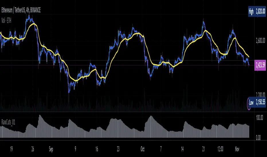
EphemerisLibrary "Ephemeris"
TODO: add library description here
mercuryElements()
mercuryRates()
venusElements()
venusRates()
earthElements()
earthRates()
marsElements()
marsRates()
jupiterElements()
jupiterRates()
saturnElements()
saturnRates()
uranusElements()
uranusRates()
neptuneElements()
neptuneRates()
rev360(x)
Normalize degrees to within [0, 360)
Parameters:
x (float) : degrees to be normalized
Returns: Normalized degrees
scaleAngle(longitude, magnitude, harmonic)
Scale angle in degrees
Parameters:
longitude (float)
magnitude (float)
harmonic (int)
Returns: Scaled angle in degrees
julianCenturyInJulianDays()
Constant Julian days per century
Returns: 36525
julianEpochJ2000()
Julian date on J2000 epoch start (2000-01-01)
Returns: 2451545.0
meanObliquityForJ2000()
Mean obliquity of the ecliptic on J2000 epoch start (2000-01-01)
Returns: 23.43928
getJulianDate(Year, Month, Day, Hour, Minute)
Convert calendar date to Julian date
Parameters:
Year (int) : calendar year as integer (e.g. 2018)
Month (int) : calendar month (January = 1, December = 12)
Day (int) : calendar day of month (e.g. January valid days are 1-31)
Hour (int) : valid values 0-23
Minute (int) : valid values 0-60
julianCenturies(date, epoch_start)
Centuries since Julian Epoch 2000-01-01
Parameters:
date (float) : Julian date to conver to Julian centuries
epoch_start (float) : Julian date of epoch start (e.g. J2000 epoch = 2451545)
Returns: Julian date converted to Julian centuries
julianCenturiesSinceEpochJ2000(julianDate)
Calculate Julian centuries since epoch J2000 (2000-01-01)
Parameters:
julianDate (float) : Julian Date in days
Returns: Julian centuries since epoch J2000 (2000-01-01)
atan2(y, x)
Specialized arctan function
Parameters:
y (float) : radians
x (float) : radians
Returns: special arctan of y/x
eccAnom(ec, m_param, dp)
Compute eccentricity of the anomaly
Parameters:
ec (float) : Eccentricity of Orbit
m_param (float) : Mean Anomaly ?
dp (int) : Decimal places to round to
Returns: Eccentricity of the Anomaly
planetEphemerisCalc(TGen, planetElementId, planetRatesId)
Compute planetary ephemeris (longtude relative to Earth or Sun) on a Julian date
Parameters:
TGen (float) : Julian Date
planetElementId (float ) : All planet orbital elements in an array. This index references a specific planet's elements.
planetRatesId (float ) : All planet orbital rates in an array. This index references a specific planet's rates.
Returns: X,Y,Z ecliptic rectangular coordinates and R radius from reference body.
calculateRightAscensionAndDeclination(earthX, earthY, earthZ, planetX, planetY, planetZ)
Calculate right ascension and declination for a planet relative to Earth
Parameters:
earthX (float) : Earth X ecliptic rectangular coordinate relative to Sun
earthY (float) : Earth Y ecliptic rectangular coordinate relative to Sun
earthZ (float) : Earth Z ecliptic rectangular coordinate relative to Sun
planetX (float) : Planet X ecliptic rectangular coordinate relative to Sun
planetY (float) : Planet Y ecliptic rectangular coordinate relative to Sun
planetZ (float) : Planet Z ecliptic rectangular coordinate relative to Sun
Returns: Planet geocentric orbital radius, geocentric right ascension, and geocentric declination
mercuryHelio(T)
Compute Mercury heliocentric longitude on date
Parameters:
T (float)
Returns: Mercury heliocentric longitude on date
venusHelio(T)
Compute Venus heliocentric longitude on date
Parameters:
T (float)
Returns: Venus heliocentric longitude on date
earthHelio(T)
Compute Earth heliocentric longitude on date
Parameters:
T (float)
Returns: Earth heliocentric longitude on date
marsHelio(T)
Compute Mars heliocentric longitude on date
Parameters:
T (float)
Returns: Mars heliocentric longitude on date
jupiterHelio(T)
Compute Jupiter heliocentric longitude on date
Parameters:
T (float)
Returns: Jupiter heliocentric longitude on date
saturnHelio(T)
Compute Saturn heliocentric longitude on date
Parameters:
T (float)
Returns: Saturn heliocentric longitude on date
neptuneHelio(T)
Compute Neptune heliocentric longitude on date
Parameters:
T (float)
Returns: Neptune heliocentric longitude on date
uranusHelio(T)
Compute Uranus heliocentric longitude on date
Parameters:
T (float)
Returns: Uranus heliocentric longitude on date
sunGeo(T)
Parameters:
T (float)
mercuryGeo(T)
Parameters:
T (float)
venusGeo(T)
Parameters:
T (float)
marsGeo(T)
Parameters:
T (float)
jupiterGeo(T)
Parameters:
T (float)
saturnGeo(T)
Parameters:
T (float)
neptuneGeo(T)
Parameters:
T (float)
uranusGeo(T)
Parameters:
T (float)
moonGeo(T_JD)
Parameters:
T_JD (float)
mercuryOrbitalPeriod()
Mercury orbital period in Earth days
Returns: 87.9691
venusOrbitalPeriod()
Venus orbital period in Earth days
Returns: 224.701
earthOrbitalPeriod()
Earth orbital period in Earth days
Returns: 365.256363004
marsOrbitalPeriod()
Mars orbital period in Earth days
Returns: 686.980
jupiterOrbitalPeriod()
Jupiter orbital period in Earth days
Returns: 4332.59
saturnOrbitalPeriod()
Saturn orbital period in Earth days
Returns: 10759.22
uranusOrbitalPeriod()
Uranus orbital period in Earth days
Returns: 30688.5
neptuneOrbitalPeriod()
Neptune orbital period in Earth days
Returns: 60195.0
jupiterSaturnCompositePeriod()
jupiterNeptuneCompositePeriod()
jupiterUranusCompositePeriod()
saturnNeptuneCompositePeriod()
saturnUranusCompositePeriod()
planetSineWave(julianDateInCenturies, planetOrbitalPeriod, planetHelio)
Convert heliocentric longitude of planet into a sine wave
Parameters:
julianDateInCenturies (float)
planetOrbitalPeriod (float) : Orbital period of planet in Earth days
planetHelio (float) : Heliocentric longitude of planet in degrees
Returns: Sine of heliocentric longitude on a Julian date

Regression Channel Alternative MTF V2█ OVERVIEW
This indicator is a predecessor to Regression Channel Alternative MTF , which is coded based on latest update of type, object and method.
█ IMPORTANT NOTES
This indicator is NOT true Multi Timeframe (MTF) but considered as Alternative MTF which calculate 100 bars for Primary MTF, can be refer from provided line helper.
The timeframe scenarios are defined based on Position, Swing and Intraday Trader.
Suppported Timeframe : W, D, 60, 15, 5 and 1.
Channel drawn based on regression calculation.
Angle channel is NOT supported.
█ INSPIRATIONS
These timeframe scenarios are defined based on Harmonic Trading : Volume Three written by Scott M Carney.
By applying channel on each timeframe, MW or ABCD patterns can be easily identified manually.
This can also be applied on other chart patterns.
█ CREDITS
Scott M Carney, Harmonic Trading : Volume Three (Reaction vs. Reversal)
█ TIMEFRAME EXPLAINED
Higher / Distal : The (next) longer or larger comparative timeframe after primary pattern has been identified.
Primary / Clear : Timeframe that possess the clearest pattern structure.
Lower / Proximate : The (next) shorter timeframe after primary pattern has been identified.
Lowest : Check primary timeframe as main reference.
█ FEATURES
Color is determined by trend or timeframe.
Some color is depends on chart contrast color.
Color is determined by trend or timeframe.
█ EXAMPLE OF USAGE / EXPLAINATION

Lyapunov Hodrick-Prescott Oscillator w/ DSL [Loxx]Lyapunov Hodrick-Prescott Oscillator w/ DSL is a Hodrick-Prescott Channel Filter that is modified using the Lyapunov stability algorithm to turn the filter into an oscillator. Signals are created using Discontinued Signal Lines.
What is the Lyapunov Stability?
As soon as scientists realized that the evolution of physical systems can be described in terms of mathematical equations, the stability of the various dynamical regimes was recognized as a matter of primary importance. The interest for this question was not only motivated by general curiosity, but also by the need to know, in the XIX century, to what extent the behavior of suitable mechanical devices remains unchanged, once their configuration has been perturbed. As a result, illustrious scientists such as Lagrange, Poisson, Maxwell and others deeply thought about ways of quantifying the stability both in general and specific contexts. The first exact definition of stability was given by the Russian mathematician Aleksandr Lyapunov who addressed the problem in his PhD Thesis in 1892, where he introduced two methods, the first of which is based on the linearization of the equations of motion and has originated what has later been termed Lyapunov exponents (LE). (Lyapunov 1992)
The interest in it suddenly skyrocketed during the Cold War period when the so-called "Second Method of Lyapunov" (see below) was found to be applicable to the stability of aerospace guidance systems which typically contain strong nonlinearities not treatable by other methods. A large number of publications appeared then and since in the control and systems literature. More recently the concept of the Lyapunov exponent (related to Lyapunov's First Method of discussing stability) has received wide interest in connection with chaos theory . Lyapunov stability methods have also been applied to finding equilibrium solutions in traffic assignment problems.
In practice, Lyapunov exponents can be computed by exploiting the natural tendency of an n-dimensional volume to align along the n most expanding subspace. From the expansion rate of an n-dimensional volume, one obtains the sum of the n largest Lyapunov exponents. Altogether, the procedure requires evolving n linearly independent perturbations and one is faced with the problem that all vectors tend to align along the same direction. However, as shown in the late '70s, this numerical instability can be counterbalanced by orthonormalizing the vectors with the help of the Gram-Schmidt procedure (Benettin et al. 1980, Shimada and Nagashima 1979) (or, equivalently with a QR decomposition). As a result, the LE λi, naturally ordered from the largest to the most negative one, can be computed: they are altogether referred to as the Lyapunov spectrum.
The Lyapunov exponent "λ" , is useful for distinguishing among the various types of orbits. It works for discrete as well as continuous systems.
λ < 0
The orbit attracts to a stable fixed point or stable periodic orbit. Negative Lyapunov exponents are characteristic of dissipative or non-conservative systems (the damped harmonic oscillator for instance). Such systems exhibit asymptotic stability; the more negative the exponent, the greater the stability. Superstable fixed points and superstable periodic points have a Lyapunov exponent of λ = −∞. This is something akin to a critically damped oscillator in that the system heads towards its equilibrium point as quickly as possible.
λ = 0
The orbit is a neutral fixed point (or an eventually fixed point). A Lyapunov exponent of zero indicates that the system is in some sort of steady state mode. A physical system with this exponent is conservative. Such systems exhibit Lyapunov stability. Take the case of two identical simple harmonic oscillators with different amplitudes. Because the frequency is independent of the amplitude, a phase portrait of the two oscillators would be a pair of concentric circles. The orbits in this situation would maintain a constant separation, like two flecks of dust fixed in place on a rotating record.
λ > 0
The orbit is unstable and chaotic. Nearby points, no matter how close, will diverge to any arbitrary separation. All neighborhoods in the phase space will eventually be visited. These points are said to be unstable. For a discrete system, the orbits will look like snow on a television set. This does not preclude any organization as a pattern may emerge. Thus the snow may be a bit lumpy. For a continuous system, the phase space would be a tangled sea of wavy lines like a pot of spaghetti. A physical example can be found in Brownian motion. Although the system is deterministic, there is no order to the orbit that ensues.
For our purposes here, we transform the HP by applying Lyapunov Stability as follows:
output = math.log(math.abs(HP / HP ))
You can read more about Lyapunov Stability here: Measuring Chaos
What is. the Hodrick-Prescott Filter?
The Hodrick-Prescott (HP) filter refers to a data-smoothing technique. The HP filter is commonly applied during analysis to remove short-term fluctuations associated with the business cycle. Removal of these short-term fluctuations reveals long-term trends.
The Hodrick-Prescott (HP) filter is a tool commonly used in macroeconomics. It is named after economists Robert Hodrick and Edward Prescott who first popularized this filter in economics in the 1990s. Hodrick was an economist who specialized in international finance. Prescott won the Nobel Memorial Prize, sharing it with another economist for their research in macroeconomics.
This filter determines the long-term trend of a time series by discounting the importance of short-term price fluctuations. In practice, the filter is used to smooth and detrend the Conference Board's Help Wanted Index (HWI) so it can be benchmarked against the Bureau of Labor Statistic's (BLS) JOLTS, an economic data series that may more accurately measure job vacancies in the U.S.
The HP filter is one of the most widely used tools in macroeconomic analysis. It tends to have favorable results if the noise is distributed normally, and when the analysis being conducted is historical.
What are DSL Discontinued Signal Line?
A lot of indicators are using signal lines in order to determine the trend (or some desired state of the indicator) easier. The idea of the signal line is easy : comparing the value to it's smoothed (slightly lagging) state, the idea of current momentum/state is made.
Discontinued signal line is inheriting that simple signal line idea and it is extending it : instead of having one signal line, more lines depending on the current value of the indicator.
"Signal" line is calculated the following way :
When a certain level is crossed into the desired direction, the EMA of that value is calculated for the desired signal line
When that level is crossed into the opposite direction, the previous "signal" line value is simply "inherited" and it becomes a kind of a level
This way it becomes a combination of signal lines and levels that are trying to combine both the good from both methods.
In simple terms, DSL uses the concept of a signal line and betters it by inheriting the previous signal line's value & makes it a level.
Included:
Bar coloring
Alerts
Signals
Loxx's Expanded Source Types

Weight Gain 4000 - (Adjustable Volume Weighted MA) - [mutantdog]Short Version:
This is a fairly self-contained system based upon a moving average crossover with several unique features. The most significant of these is the adjustable volume weighting system, allowing for transformations between standard and weighted versions of each included MA. With this feature it is possible to apply partial weighting which can help to improve responsiveness without dramatically altering shape. Included types are SMA, EMA, WMA, RMA, hSMA, DEMA and TEMA. Potentially more will be added in future (check updates below).
In addition there are a selection of alternative 'weighted' inputs, a pair of Bollinger-style deviation bands, a separate price tracker and a bunch of alert presets.
This can be used out-of-the-box or tweaked in multiple ways for unusual results. Default settings are a basic 8/21 EMA cross with partial volume weighting. Dev bands apply to MA2 and are based upon the type and the volume weighting. For standard Bollinger bands use SMA with length 20 and try adding a small amount of volume weighting.
A more detailed breakdown of the functionality follows.
Long Version:
ADJUSTABLE VOLUME WEIGHTING
In principle any moving average should have a volume weighted analogue, the standard VWMA is just an SMA with volume weighting for example. Actually, we can consider the SMA to be a special case where volume is a constant 1 per bar (the value is somewhat arbitrary, the important part is that it's constant). Similar principles apply to the 'elastic' EVWMA which is the volume weighted analogue of an RMA. In any case though, where we have standard and weighted variants it is possible to transform one into the other by gradually increasing or decreasing the weighting, which forms the basis of this system. This is not just a simple multiplier however, that would not work due to the relative proportions being the same when set at any non zero value. In order to create a meaningful transformation we need to use an exponent instead, eg: volume^x , where x is a variable determined in this case by the 'volume' parameter. When x=1, the full volume weighting applies and when x=0, the volume will be reduced to a constant 1. Values in between will result in the respective partial weighting, for example 0.5 will give the square root of the volume.
The obvious question here though is why would you want to do this? To answer that really it is best to actually try it. The advantages that volume weighting can bring to a moving average can sometimes come at the cost of unwanted or erratic behaviour. While it can tend towards much closer price tracking which may be desirable, sometimes it needs moderating especially in markets with lower liquidity. Here the adjustability can be useful, in many cases i have found that adding a small amount of volume weighting to a chosen MA can help to improve its responsiveness without overpowering it. Another possible use case would be to have two instances of the same MA with the same length but different weightings, the extent to which these diverge from each other can be a useful indicator of trend strength. Other uses will become apparent with experimentation and can vary from one market to another.
THE INCLUDED MODES
At the time of publication, there are 7 included moving average types with plans to add more in future. For now here is a brief explainer of what's on offer (continuing to use x as shorthand for the volume parameter), starting with the two most common types.
SMA: As mentioned above this is essentially a standard VWMA, calculated here as sma(source*volume^x,length)/sma(volume^x,length). In this case when x=0 then volume=1 and it reduces to a standard SMA.
RMA: Again mentioned above, this is an EVWMA (where E stands for elastic) with constant weighting. Without going into detail, this method takes the 1/length factor of an RMA and replaces it with volume^x/sum(volume^x,length). In this case again we can see that when x=0 then volume=1 and the original 1/length factor is restored.
EMA: This follows the same principle as the RMA where the standard 2/(length+1) factor is replaced with (2*volume^x)/(sum(volume^x,length)+volume^x). As with an RMA, when x=0 then volume=1 and this reduces back to the standard 2/(length+1).
DEMA: Just a standard Double EMA using the above.
TEMA: Likewise, a standard Triple EMA using the above.
hSMA: This is the same as the SMA except it uses harmonic mean calculations instead of arithmetic. In most cases the differences are negligible however they can become more pronounced when volume weighting is introduced. Furthermore, an argument can be made that harmonic mean calculations are better suited to downtrends or bear markets, in principle at least.
WMA: Probably the most contentious one included. Follows the same basic calculations as for the SMA except uses a WMA instead. Honestly, it makes little sense to combine both linear and volume weighting in this manner, included only for completeness and because it can easily be done. It may be the case that a superior composite could be created with some more complex calculations, in which case i may add that later. For now though this will do.
An additional 'volume filter' option is included, which applies a basic filter to the volume prior to calculation. For types based around the SMA/VWMA system, the volume filter is a WMA-4, for types based around the RMA/EVWMA system the filter is a RMA-2.
As and when i add more they will be listed in the updates at the bottom.
WEIGHTED INPUTS
The ohlc method of source calculations is really a leftover from a time when data was far more limited. Nevertheless it is still the method used in charting and for the most part is sufficient. Often the only important value is 'close' although sometimes 'high' and 'low' can be relevant also. Since we are volume weighting however, it can be useful to incorporate as much information as possible. To that end either 'hlc3' or 'hlcc4' tend to be the best of the defaults (in the case of 24/7 charting like crypto or intraday trading, 'ohlc4' should be avoided as it is effectively the same as a lagging version of 'hlcc4'). There are many other (infinitely many, in fact) possible combinations that can be created, i have included a few here.
The premise is fairly straightforward, by subtracting one value from another, the remaining difference can act as a kind of weight. In a simple case consider 'hl2' as simply the midrange ((high+low)/2), instead of this using 'high+low-open' would give more weight to the value furthest from the open, providing a good estimate of the median. An even better estimate can be achieved by combining that with 'high+low-close' to give the included result 'hl-oc2'. Similarly, 'hlc3' can be considered the basic mean of the three significant values, an included weighted version 'hlc2-o2' combines a sum with subtraction of open to give an estimated mean that may be more accurate. Finally we can apply a similar principle to the close, by subtracting the other values, this one potentially gets more complex so the included 'cc-ohlc4' is really the simplest. The result here is an overbias of the close in relation to the open and the midrange, while in most cases not as useful it can provide an estimate for the next bar assuming that the trend continues.
Of the three i've included, hlc2-o2 is in my opinion the most useful especially in this context, although it is perhaps best considered to be experimental in nature. For that reason, i've kept 'hlcc4' as the default for both MAs.
Additionally included is an 'aux input' which is the standard TV source menu and, where possible, can be set as outputs of other indicators.
THE SYSTEM
This one is fairly obvious and straightforward. It's just a moving average crossover with additional deviation (bollinger) bands. Not a lot to explain here as it should be apparent how it works.
Of the two, MA1 is considered to be the fast and MA2 is considered to be the slow. Both can be set with independent inputs, types and weighting. When MA1 is above, the colour of both is green and when it's below the colour of both is red. An additional gradient based fill is there and can be adjusted along with everything else in the visuals section at the bottom. Default alerts are available for crossover/crossunder conditions along with optional marker plots.
MA2 has the option for deviation bands, these are calculated based upon the MA type used and volume weighted according to the main parameter. In the case of a unweighted SMA being used they will be standard Bollinger bands.
An additional 'source direct' price tracker is included which can be used as the basis for an alert system for price crossings of bands or MAs, while taking advantage of the available weighted inputs. This is displayed as a stepped line on the chart so is also a good way to visualise the differences between input types.
That just about covers it then. The likelihood is that you've used some sort of moving average cross system before and are probably still using one or more. If so, then perhaps the additional functionality here will be of benefit.
Thanks for looking, I welcome any feedack
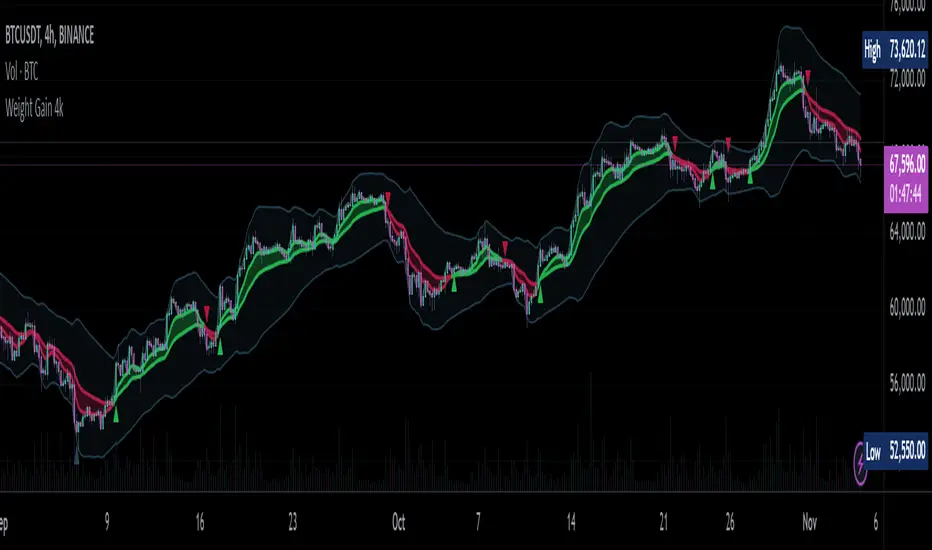
HarmonicDB█ OVERVIEW
This library was to showcase database for specifications of Harmonic Patterns using arrays.
█ CREDITS
Scott M Carney, author of Harmonic Trading : Volume Three
animal_db(x)
TODO: export animal_db
Parameters:
x : TODO: float value is set to default if not necessary
Returns: TODO:

PivotsLibrary "Pivots"
This Library focuses in functions related to pivot highs and lows and some of their applications (i.e. divergences, zigzag, harmonics, support and resistance...)
pivots(srcH, srcL, length) Delivers series of pivot highs, lows and zigzag.
Parameters:
srcH : Source series to look for pivot highs. Stricter applications might source from 'close' prices. Oscillators are also another possible source to look for pivot highs and lows. By default 'high'
srcL : Source series to look for pivot lows. By default 'low'
length : This value represents the minimum number of candles between pivots. The lower the number, the more detailed the pivot profile. The higher the number, the more relevant the pivots. By default 10
Returns:
zigzagArray(pivotHigh, pivotLow) Delivers a Zigzag series based on alternating pivots. Ocasionally this line could paint a few consecutive lows or highs without alternating. That happens because it's finding a few consecutive Higher Highs or Lower Lows. If to use lines entities instead of series, that could be easily avoided. But in this one, I'm more interested outputting series rather than painting/deleting line entities.
Parameters:
pivotHigh : Pivot high series
pivotLow : Pivot low series
Returns:
zigzagLine(srcH, srcL, colorLine, widthLine) Delivers a Zigzag based on line entities.
Parameters:
srcH : Source series to look for pivot highs. Stricter applications might source from 'close' prices. Oscillators are also another possible source to look for pivot highs and lows. By default 'high'
srcL : Source series to look for pivot lows. By default 'low'
colorLine : Color of the Zigzag Line. By default Fuchsia
widthLine : Width of the Zigzag Line. By default 4
Returns: Zigzag printed on screen
divergence(h2, l2, h1, l1, length) Calculates divergences between 2 series
Parameters:
h2 : Series in which to locate divs: Highs
l2 : Series in which to locate divs: Lows
h1 : Series in which to locate pivots: Highs. By default high
l1 : Series in which to locate pivots: Lows. By default low
length : Length used to calculate Pivots: By default 10
Returns:

AB=CD Reciprocal Ratios Table (Source Code)This table indicator was intended as helper / reference for using ABCD Pattern.
Indikator berjadual bertujuan sebagai bantuan / rujukan untuk kegunaan ABCD Pattern.
The values shown in table was based on Harmonic Trading : Volume One book written by Scott M Carney.
Details of value, refer Chapter 4 : The AB=CD Pattern (Page 41).
These values are known as AB=CD Reciprocal Ratios.
Nilai yang ditunjukkan dalam jadual adalah berdasarkan buku Harmonic Trading : Volume One ditulis oleh Scott M Carney.
Nilai secara menyeluruh, rujuk Chapter 4 : The AB=CD Pattern (Muka surat 41).
Nilai berikut dipanggil sebagai AB=CD Reciprocal Ratios
Indicator features :
1. List AB=CD Reciprocal Ratios.
2. Font size small for mobile app and font size normal for desktop.
Kemampuan indikator :
1. Senarai AB=CD Reciprocal Ratio.
2. Saiz font kecil untuk mobile app dan saiz size normal untuk desktop.
FAQ
1. Credits / Kredit
Scott M Carney,
2. Code Usage / Penggunaan Kod
Free to use for personal usage but credits are most welcomed especially for credits to Scott M Carney/
Bebas untuk kegunaan peribadi tetapi kredit adalah amat dialu-alukan terutamanya kredit kepada Scott M Carney.
Settings with appropriate value.
Setting dengan nilai yang sesuai.
Default Settings.
Setting asal.
Settings with different table position.
Setting dengan posisi jadual yang berbeza.
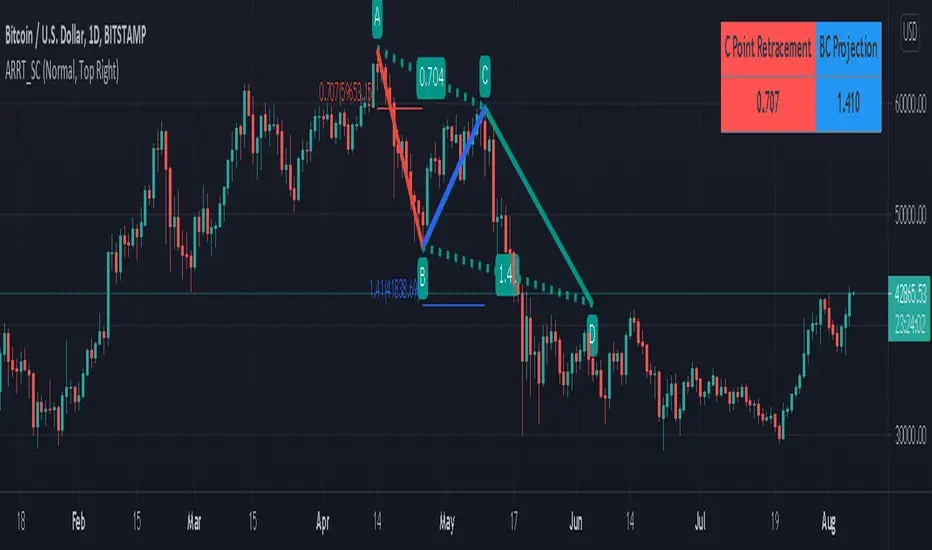
Using The AM/GM Inequality To Estimate VolatilityA volatility indicator derived from the AM/GM inequality. I don't think it will be necessary to describe the usage and interpretation of such indicator, and I don't think it is super useful, however, this is not the case of the script, which contains three ways to compute the geometric mean, with a classic, a simple, and an efficient way. The AM/GM inequality is also a really interesting concept, and I'll try to"prove" it in this post by using DSP. I also added more comments in the script in order to highlight some stuff.
The AM/GM Inequality
When we talk about the mean, we are referring to the "arithmetic" one by default, but there exist more types of means. Two other ones include the "geometric" and "harmonic" means, both are part of the Pythagorean means with the arithmetic mean.
Each one of them as several properties, but the most interesting aspect is their inequality, that is:
HM <= GM <= AM
The arithmetic mean is the one with the highest value, while the harmonic mean is the one with the lowest value. In the case each data point is equal to each other, all the means have the same value.
In our case, the inequality of interest is the inequality between the geometric and arithmetic mean, where the geometric mean is lower or equal than the arithmetic one. Many proofs/explanations exist, I'll try my version using DSP, where instead of thinking about means, we think about rolling means, which allows us to interpret them as low-pass filters. So we end up having the geometric moving average (GMA) and arithmetic moving average (SMA).
We know that GMA <= SMA , the SMA has a unity passband, this implies that the GMA has a passband lower than 1 (for non-equal input values), this explains why the GMA is smaller than the SMA. In order for a FIR filter to have a passband lower than 1, the sum of the filter coefficients must be lower than 1. In order to further proves this consider the following equation:
sqrt(a×b) = k×a + k×b
Here sqrt(a×b) is the geometric mean of a and b , the right-hand side of the equation is a weighted sum between a and b and coefficient k , we want to solve the equation with respect to k , if k×2 < 1 then we have the proof that GMA < SMA . The solution with respect to k is:
k = sqrt(a×b)/(a+b)
which always gives a number lower than 0.5, as such k×2 < 1 and thus the passband is lower than 1. If our input values are equal to each other, we end up with the following solution for k :
k = sqrt(a×a)/(a+a) = a/(2×a) = 0.5
as such the GMA has the coefficients of an SMA as long as the input values are equal to each other.
Because of this inequality, we can subtract the SMA to a GMA and take the square root of the result in order to have a volatility indicator, however, both moving averages are still pretty close to each other, which gives a very small result for the indicator.
Uwu I am a bit tired, better indicators coming up
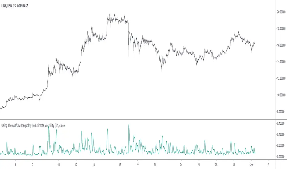
Musical Harmonics - Start with a low.Octaves double from one octave to another, so start with octaves beginning with the number one, for example:
1 doubled is 2, 2 doubled is 4, 4 double is 8 and then we go on to this sequence:
1,2,4,8,16,32,64,126,256,512,1024,2048,etc,etc
Find one of the numbers near a range, so for example on this chart Ethereum was trading at 190.31. That price is in between the octaves of 126 and 256. The number I use as the low for the indicator is 126.
Working on updating with labels and such
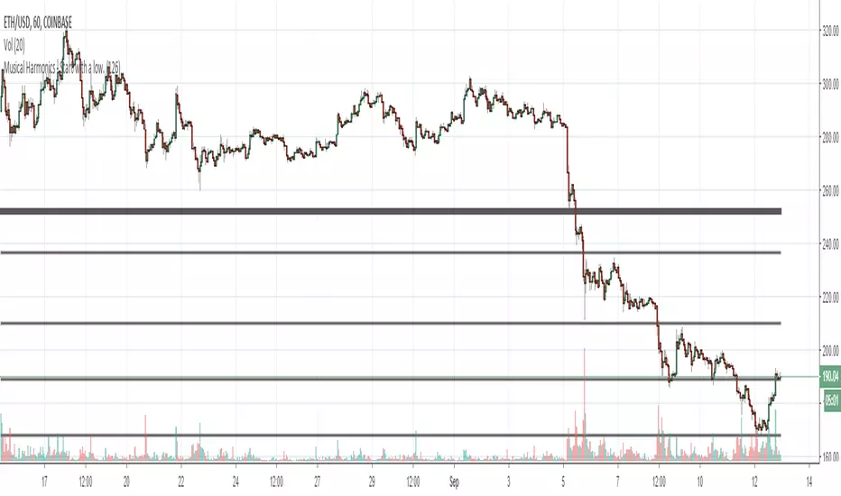
Adaptive Market Wave TheoryAdaptive Market Wave Theory
🌊 CORE INNOVATION: PROBABILISTIC PHASE DETECTION WITH MULTI-AGENT CONSENSUS
Adaptive Market Wave Theory (AMWT) represents a fundamental paradigm shift in how traders approach market phase identification. Rather than counting waves subjectively or drawing static breakout levels, AMWT treats the market as a hidden state machine —using Hidden Markov Models, multi-agent consensus systems, and reinforcement learning algorithms to quantify what traditional methods leave to interpretation.
The Wave Analysis Problem:
Traditional wave counting methodologies (Elliott Wave, harmonic patterns, ABC corrections) share fatal weaknesses that AMWT directly addresses:
1. Non-Falsifiability : Invalid wave counts can always be "recounted" or "adjusted." If your Wave 3 fails, it becomes "Wave 3 of a larger degree" or "actually Wave C." There's no objective failure condition.
2. Observer Bias : Two expert wave analysts examining the same chart routinely reach different conclusions. This isn't a feature—it's a fundamental methodology flaw.
3. No Confidence Measure : Traditional analysis says "This IS Wave 3." But with what probability? 51%? 95%? The binary nature prevents proper position sizing and risk management.
4. Static Rules : Fixed Fibonacci ratios and wave guidelines cannot adapt to changing market regimes. What worked in 2019 may fail in 2024.
5. No Accountability : Wave methodologies rarely track their own performance. There's no feedback loop to improve.
The AMWT Solution:
AMWT addresses each limitation through rigorous mathematical frameworks borrowed from speech recognition, machine learning, and reinforcement learning:
• Non-Falsifiability → Hard Invalidation : Wave hypotheses die permanently when price violates calculated invalidation levels. No recounting allowed.
• Observer Bias → Multi-Agent Consensus : Three independent analytical agents must agree. Single-methodology bias is eliminated.
• No Confidence → Probabilistic States : Every market state has a calculated probability from Hidden Markov Model inference. "72% probability of impulse state" replaces "This is Wave 3."
• Static Rules → Adaptive Learning : Thompson Sampling multi-armed bandits learn which agents perform best in current conditions. The system adapts in real-time.
• No Accountability → Performance Tracking : Comprehensive statistics track every signal's outcome. The system knows its own performance.
The Core Insight:
"Traditional wave analysis asks 'What count is this?' AMWT asks 'What is the probability we are in an impulsive state, with what confidence, confirmed by how many independent methodologies, and anchored to what liquidity event?'"
🔬 THEORETICAL FOUNDATION: HIDDEN MARKOV MODELS
Why Hidden Markov Models?
Markets exist in hidden states that we cannot directly observe—only their effects on price are visible. When the market is in an "impulse up" state, we see rising prices, expanding volume, and trending indicators. But we don't observe the state itself—we infer it from observables.
This is precisely the problem Hidden Markov Models (HMMs) solve. Originally developed for speech recognition (inferring words from sound waves), HMMs excel at estimating hidden states from noisy observations.
HMM Components:
1. Hidden States (S) : The unobservable market conditions
2. Observations (O) : What we can measure (price, volume, indicators)
3. Transition Matrix (A) : Probability of moving between states
4. Emission Matrix (B) : Probability of observations given each state
5. Initial Distribution (π) : Starting state probabilities
AMWT's Six Market States:
State 0: IMPULSE_UP
• Definition: Strong bullish momentum with high participation
• Observable Signatures: Rising prices, expanding volume, RSI >60, price above upper Bollinger Band, MACD histogram positive and rising
• Typical Duration: 5-20 bars depending on timeframe
• What It Means: Institutional buying pressure, trend acceleration phase
State 1: IMPULSE_DN
• Definition: Strong bearish momentum with high participation
• Observable Signatures: Falling prices, expanding volume, RSI <40, price below lower Bollinger Band, MACD histogram negative and falling
• Typical Duration: 5-20 bars (often shorter than bullish impulses—markets fall faster)
• What It Means: Institutional selling pressure, panic or distribution acceleration
State 2: CORRECTION
• Definition: Counter-trend consolidation with declining momentum
• Observable Signatures: Sideways or mild counter-trend movement, contracting volume, RSI returning toward 50, Bollinger Bands narrowing
• Typical Duration: 8-30 bars
• What It Means: Profit-taking, digestion of prior move, potential accumulation for next leg
State 3: ACCUMULATION
• Definition: Base-building near lows where informed participants absorb supply
• Observable Signatures: Price near recent lows but not making new lows, volume spikes on up bars, RSI showing positive divergence, tight range
• Typical Duration: 15-50 bars
• What It Means: Smart money buying from weak hands, preparing for markup phase
State 4: DISTRIBUTION
• Definition: Top-forming near highs where informed participants distribute holdings
• Observable Signatures: Price near recent highs but struggling to advance, volume spikes on down bars, RSI showing negative divergence, widening range
• Typical Duration: 15-50 bars
• What It Means: Smart money selling to late buyers, preparing for markdown phase
State 5: TRANSITION
• Definition: Regime change period with mixed signals and elevated uncertainty
• Observable Signatures: Conflicting indicators, whipsaw price action, no clear momentum, high volatility without direction
• Typical Duration: 5-15 bars
• What It Means: Market deciding next direction, dangerous for directional trades
The Transition Matrix:
The transition matrix A captures the probability of moving from one state to another. AMWT initializes with empirically-derived values then updates online:
From/To IMP_UP IMP_DN CORR ACCUM DIST TRANS
IMP_UP 0.70 0.02 0.20 0.02 0.04 0.02
IMP_DN 0.02 0.70 0.20 0.04 0.02 0.02
CORR 0.15 0.15 0.50 0.10 0.10 0.00
ACCUM 0.30 0.05 0.15 0.40 0.05 0.05
DIST 0.05 0.30 0.15 0.05 0.40 0.05
TRANS 0.20 0.20 0.20 0.15 0.15 0.10
Key Insights from Transition Probabilities:
• Impulse states are sticky (70% self-transition): Once trending, markets tend to continue
• Corrections can transition to either impulse direction (15% each): The next move after correction is uncertain
• Accumulation strongly favors IMP_UP transition (30%): Base-building leads to rallies
• Distribution strongly favors IMP_DN transition (30%): Topping leads to declines
The Viterbi Algorithm:
Given a sequence of observations, how do we find the most likely state sequence? This is the Viterbi algorithm—dynamic programming to find the optimal path through the state space.
Mathematical Formulation:
δ_t(j) = max_i × B_j(O_t)
Where:
δ_t(j) = probability of most likely path ending in state j at time t
A_ij = transition probability from state i to state j
B_j(O_t) = emission probability of observation O_t given state j
AMWT Implementation:
AMWT runs Viterbi over a rolling window (default 50 bars), computing the most likely state sequence and extracting:
• Current state estimate
• State confidence (probability of current state vs alternatives)
• State sequence for pattern detection
Online Learning (Baum-Welch Adaptation):
Unlike static HMMs, AMWT continuously updates its transition and emission matrices based on observed market behavior:
f_onlineUpdateHMM(prev_state, curr_state, observation, decay) =>
// Update transition matrix
A *= decay
A += (1.0 - decay)
// Renormalize row
// Update emission matrix
B *= decay
B += (1.0 - decay)
// Renormalize row
The decay parameter (default 0.85) controls adaptation speed:
• Higher decay (0.95): Slower adaptation, more stable, better for consistent markets
• Lower decay (0.80): Faster adaptation, more reactive, better for regime changes
Why This Matters for Trading:
Traditional indicators give you a number (RSI = 72). AMWT gives you a probabilistic state assessment :
"There is a 78% probability we are in IMPULSE_UP state, with 15% probability of CORRECTION and 7% distributed among other states. The transition matrix suggests 70% chance of remaining in IMPULSE_UP next bar, 20% chance of transitioning to CORRECTION."
This enables:
• Position sizing by confidence : 90% confidence = full size; 60% confidence = half size
• Risk management by transition probability : High correction probability = tighten stops
• Strategy selection by state : IMPULSE = trend-follow; CORRECTION = wait; ACCUMULATION = scale in
🎰 THE 3-BANDIT CONSENSUS SYSTEM
The Multi-Agent Philosophy:
No single analytical methodology works in all market conditions. Trend-following excels in trending markets but gets chopped in ranges. Mean-reversion excels in ranges but gets crushed in trends. Structure-based analysis works when structure is clear but fails in chaotic markets.
AMWT's solution: employ three independent agents , each analyzing the market from a different perspective, then use Thompson Sampling to learn which agents perform best in current conditions.
Agent 1: TREND AGENT
Philosophy : Markets trend. Follow the trend until it ends.
Analytical Components:
• EMA Alignment: EMA8 > EMA21 > EMA50 (bullish) or inverse (bearish)
• MACD Histogram: Direction and rate of change
• Price Momentum: Close relative to ATR-normalized movement
• VWAP Position: Price above/below volume-weighted average price
Signal Generation:
Strong Bull: EMA aligned bull AND MACD histogram > 0 AND momentum > 0.3 AND close > VWAP
→ Signal: +1 (Long), Confidence: 0.75 + |momentum| × 0.4
Moderate Bull: EMA stack bull AND MACD rising AND momentum > 0.1
→ Signal: +1 (Long), Confidence: 0.65 + |momentum| × 0.3
Strong Bear: EMA aligned bear AND MACD histogram < 0 AND momentum < -0.3 AND close < VWAP
→ Signal: -1 (Short), Confidence: 0.75 + |momentum| × 0.4
Moderate Bear: EMA stack bear AND MACD falling AND momentum < -0.1
→ Signal: -1 (Short), Confidence: 0.65 + |momentum| × 0.3
When Trend Agent Excels:
• Trend days (IB extension >1.5x)
• Post-breakout continuation
• Institutional accumulation/distribution phases
When Trend Agent Fails:
• Range-bound markets (ADX <20)
• Chop zones after volatility spikes
• Reversal days at major levels
Agent 2: REVERSION AGENT
Philosophy: Markets revert to mean. Extreme readings reverse.
Analytical Components:
• Bollinger Band Position: Distance from bands, percent B
• RSI Extremes: Overbought (>70) and oversold (<30)
• Stochastic: %K/%D crossovers at extremes
• Band Squeeze: Bollinger Band width contraction
Signal Generation:
Oversold Bounce: BB %B < 0.20 AND RSI < 35 AND Stochastic < 25
→ Signal: +1 (Long), Confidence: 0.70 + (30 - RSI) × 0.01
Overbought Fade: BB %B > 0.80 AND RSI > 65 AND Stochastic > 75
→ Signal: -1 (Short), Confidence: 0.70 + (RSI - 70) × 0.01
Squeeze Fire Bull: Band squeeze ending AND close > upper band
→ Signal: +1 (Long), Confidence: 0.65
Squeeze Fire Bear: Band squeeze ending AND close < lower band
→ Signal: -1 (Short), Confidence: 0.65
When Reversion Agent Excels:
• Rotation days (price stays within IB)
• Range-bound consolidation
• After extended moves without pullback
When Reversion Agent Fails:
• Strong trend days (RSI can stay overbought for days)
• Breakout moves
• News-driven directional moves
Agent 3: STRUCTURE AGENT
Philosophy: Market structure reveals institutional intent. Follow the smart money.
Analytical Components:
• Break of Structure (BOS): Price breaks prior swing high/low
• Change of Character (CHOCH): First break against prevailing trend
• Higher Highs/Higher Lows: Bullish structure
• Lower Highs/Lower Lows: Bearish structure
• Liquidity Sweeps: Stop runs that reverse
Signal Generation:
BOS Bull: Price breaks above prior swing high with momentum
→ Signal: +1 (Long), Confidence: 0.70 + structure_strength × 0.2
CHOCH Bull: First higher low after downtrend, breaking structure
→ Signal: +1 (Long), Confidence: 0.75
BOS Bear: Price breaks below prior swing low with momentum
→ Signal: -1 (Short), Confidence: 0.70 + structure_strength × 0.2
CHOCH Bear: First lower high after uptrend, breaking structure
→ Signal: -1 (Short), Confidence: 0.75
Liquidity Sweep Long: Price sweeps below swing low then reverses strongly
→ Signal: +1 (Long), Confidence: 0.80
Liquidity Sweep Short: Price sweeps above swing high then reverses strongly
→ Signal: -1 (Short), Confidence: 0.80
When Structure Agent Excels:
• After liquidity grabs (stop runs)
• At major swing points
• During institutional accumulation/distribution
When Structure Agent Fails:
• Choppy, structureless markets
• During news events (structure becomes noise)
• Very low timeframes (noise overwhelms structure)
Thompson Sampling: The Bandit Algorithm
With three agents giving potentially different signals, how do we decide which to trust? This is the multi-armed bandit problem —balancing exploitation (using what works) with exploration (testing alternatives).
Thompson Sampling Solution:
Each agent maintains a Beta distribution representing its success/failure history:
Agent success rate modeled as Beta(α, β)
Where:
α = number of successful signals + 1
β = number of failed signals + 1
On Each Bar:
1. Sample from each agent's Beta distribution
2. Weight agent signals by sampled probabilities
3. Combine weighted signals into consensus
4. Update α/β based on trade outcomes
Mathematical Implementation:
// Beta sampling via Gamma ratio method
f_beta_sample(alpha, beta) =>
g1 = f_gamma_sample(alpha)
g2 = f_gamma_sample(beta)
g1 / (g1 + g2)
// Thompson Sampling selection
for each agent:
sampled_prob = f_beta_sample(agent.alpha, agent.beta)
weight = sampled_prob / sum(all_sampled_probs)
consensus += agent.signal × agent.confidence × weight
Why Thompson Sampling?
• Automatic Exploration : Agents with few samples get occasional chances (high variance in Beta distribution)
• Bayesian Optimal : Mathematically proven optimal solution to exploration-exploitation tradeoff
• Uncertainty-Aware : Small sample size = more exploration; large sample size = more exploitation
• Self-Correcting : Poor performers naturally get lower weights over time
Example Evolution:
Day 1 (Initial):
Trend Agent: Beta(1,1) → samples ~0.50 (high uncertainty)
Reversion Agent: Beta(1,1) → samples ~0.50 (high uncertainty)
Structure Agent: Beta(1,1) → samples ~0.50 (high uncertainty)
After 50 Signals:
Trend Agent: Beta(28,23) → samples ~0.55 (moderate confidence)
Reversion Agent: Beta(18,33) → samples ~0.35 (underperforming)
Structure Agent: Beta(32,19) → samples ~0.63 (outperforming)
Result: Structure Agent now receives highest weight in consensus
Consensus Requirements by Mode:
Aggressive Mode:
• Minimum 1/3 agents agreeing
• Consensus threshold: 45%
• Use case: More signals, higher risk tolerance
Balanced Mode:
• Minimum 2/3 agents agreeing
• Consensus threshold: 55%
• Use case: Standard trading
Conservative Mode:
• Minimum 2/3 agents agreeing
• Consensus threshold: 65%
• Use case: Higher quality, fewer signals
Institutional Mode:
• Minimum 2/3 agents agreeing
• Consensus threshold: 75%
• Additional: Session quality >0.65, mode adjustment +0.10
• Use case: Highest quality signals only
🌀 INTELLIGENT CHOP DETECTION ENGINE
The Chop Problem:
Most trading losses occur not from being wrong about direction, but from trading in conditions where direction doesn't exist . Choppy, range-bound markets generate false signals from every methodology—trend-following, mean-reversion, and structure-based alike.
AMWT's chop detection engine identifies these low-probability environments before signals fire, preventing the most damaging trades.
Five-Factor Chop Analysis:
Factor 1: ADX Component (25% weight)
ADX (Average Directional Index) measures trend strength regardless of direction.
ADX < 15: Very weak trend (high chop score)
ADX 15-20: Weak trend (moderate chop score)
ADX 20-25: Developing trend (low chop score)
ADX > 25: Strong trend (minimal chop score)
adx_chop = (i_adxThreshold - adx_val) / i_adxThreshold × 100
Why ADX Works: ADX synthesizes +DI and -DI movements. Low ADX means price is moving but not directionally—the definition of chop.
Factor 2: Choppiness Index (25% weight)
The Choppiness Index measures price efficiency using the ratio of ATR sum to price range:
CI = 100 × LOG10(SUM(ATR, n) / (Highest - Lowest)) / LOG10(n)
CI > 61.8: Choppy (range-bound, inefficient movement)
CI < 38.2: Trending (directional, efficient movement)
CI 38.2-61.8: Transitional
chop_idx_score = (ci_val - 38.2) / (61.8 - 38.2) × 100
Why Choppiness Index Works: In trending markets, price covers distance efficiently (low ATR sum relative to range). In choppy markets, price oscillates wildly but goes nowhere (high ATR sum relative to range).
Factor 3: Range Compression (20% weight)
Compares recent range to longer-term range, detecting volatility squeezes:
recent_range = Highest(20) - Lowest(20)
longer_range = Highest(50) - Lowest(50)
compression = 1 - (recent_range / longer_range)
compression > 0.5: Strong squeeze (potential breakout imminent)
compression < 0.2: No compression (normal volatility)
range_compression_score = compression × 100
Why Range Compression Matters: Compression precedes expansion. High compression = market coiling, preparing for move. Signals during compression often fail because the breakout hasn't occurred yet.
Factor 4: Channel Position (15% weight)
Tracks price position within the macro channel:
channel_position = (close - channel_low) / (channel_high - channel_low)
position 0.4-0.6: Center of channel (indecision zone)
position <0.2 or >0.8: Near extremes (potential reversal or breakout)
channel_chop = abs(0.5 - channel_position) < 0.15 ? high_score : low_score
Why Channel Position Matters: Price in the middle of a range is in "no man's land"—equally likely to go either direction. Signals in the channel center have lower probability.
Factor 5: Volume Quality (15% weight)
Assesses volume relative to average:
vol_ratio = volume / SMA(volume, 20)
vol_ratio < 0.7: Low volume (lack of conviction)
vol_ratio 0.7-1.3: Normal volume
vol_ratio > 1.3: High volume (conviction present)
volume_chop = vol_ratio < 0.8 ? (1 - vol_ratio) × 100 : 0
Why Volume Quality Matters: Low volume moves lack institutional participation. These moves are more likely to reverse or stall.
Combined Chop Intensity:
chopIntensity = (adx_chop × 0.25) + (chop_idx_score × 0.25) +
(range_compression_score × 0.20) + (channel_chop × 0.15) +
(volume_chop × i_volumeChopWeight × 0.15)
Regime Classifications:
Based on chop intensity and component analysis:
• Strong Trend (0-20%): ADX >30, clear directional momentum, trade aggressively
• Trending (20-35%): ADX >20, moderate directional bias, trade normally
• Transitioning (35-50%): Mixed signals, regime change possible, reduce size
• Mid-Range (50-60%): Price trapped in channel center, avoid new positions
• Ranging (60-70%): Low ADX, price oscillating within bounds, fade extremes only
• Compression (70-80%): Volatility squeeze, expansion imminent, wait for breakout
• Strong Chop (80-100%): Multiple chop factors aligned, avoid trading entirely
Signal Suppression:
When chop intensity exceeds the configurable threshold (default 80%), signals are suppressed entirely. The dashboard displays "⚠️ CHOP ZONE" with the current regime classification.
Chop Box Visualization:
When chop is detected, AMWT draws a semi-transparent box on the chart showing the chop zone. This visual reminder helps traders avoid entering positions during unfavorable conditions.
💧 LIQUIDITY ANCHORING SYSTEM
The Liquidity Concept:
Markets move from liquidity pool to liquidity pool. Stop losses cluster at predictable locations—below swing lows (buy stops become sell orders when triggered) and above swing highs (sell stops become buy orders when triggered). Institutions know where these clusters are and often engineer moves to trigger them before reversing.
AMWT identifies and tracks these liquidity events, using them as anchors for signal confidence.
Liquidity Event Types:
Type 1: Volume Spikes
Definition: Volume > SMA(volume, 20) × i_volThreshold (default 2.8x)
Interpretation: Sudden volume surge indicates institutional activity
• Near swing low + reversal: Likely accumulation
• Near swing high + reversal: Likely distribution
• With continuation: Institutional conviction in direction
Type 2: Stop Runs (Liquidity Sweeps)
Definition: Price briefly exceeds swing high/low then reverses within N bars
Detection:
• Price breaks above recent swing high (triggering buy stops)
• Then closes back below that high within 3 bars
• Signal: Bullish stop run complete, reversal likely
Or inverse for bearish:
• Price breaks below recent swing low (triggering sell stops)
• Then closes back above that low within 3 bars
• Signal: Bearish stop run complete, reversal likely
Type 3: Absorption Events
Definition: High volume with small candle body
Detection:
• Volume > 2x average
• Candle body < 30% of candle range
• Interpretation: Large orders being filled without moving price
• Implication: Accumulation (at lows) or distribution (at highs)
Type 4: BSL/SSL Pools (Buy-Side/Sell-Side Liquidity)
BSL (Buy-Side Liquidity):
• Cluster of swing highs within ATR proximity
• Stop losses from shorts sit above these highs
• Breaking BSL triggers short covering (fuel for rally)
SSL (Sell-Side Liquidity):
• Cluster of swing lows within ATR proximity
• Stop losses from longs sit below these lows
• Breaking SSL triggers long liquidation (fuel for decline)
Liquidity Pool Mapping:
AMWT continuously scans for and maps liquidity pools:
// Detect swing highs/lows using pivot function
swing_high = ta.pivothigh(high, 5, 5)
swing_low = ta.pivotlow(low, 5, 5)
// Track recent swing points
if not na(swing_high)
bsl_levels.push(swing_high)
if not na(swing_low)
ssl_levels.push(swing_low)
// Display on chart with labels
Confluence Scoring Integration:
When signals fire near identified liquidity events, confluence scoring increases:
• Signal near volume spike: +10% confidence
• Signal after liquidity sweep: +15% confidence
• Signal at BSL/SSL pool: +10% confidence
• Signal aligned with absorption zone: +10% confidence
Why Liquidity Anchoring Matters:
Signals "in a vacuum" have lower probability than signals anchored to institutional activity. A long signal after a liquidity sweep below swing lows has trapped shorts providing fuel. A long signal in the middle of nowhere has no such catalyst.
📊 SIGNAL GRADING SYSTEM
The Quality Problem:
Not all signals are created equal. A signal with 6/6 factors aligned is fundamentally different from a signal with 3/6 factors aligned. Traditional indicators treat them the same. AMWT grades every signal based on confluence.
Confluence Components (100 points total):
1. Bandit Consensus Strength (25 points)
consensus_str = weighted average of agent confidences
score = consensus_str × 25
Example:
Trend Agent: +1 signal, 0.80 confidence, 0.35 weight
Reversion Agent: 0 signal, 0.50 confidence, 0.25 weight
Structure Agent: +1 signal, 0.75 confidence, 0.40 weight
Weighted consensus = (0.80×0.35 + 0×0.25 + 0.75×0.40) / (0.35 + 0.40) = 0.77
Score = 0.77 × 25 = 19.25 points
2. HMM State Confidence (15 points)
score = hmm_confidence × 15
Example:
HMM reports 82% probability of IMPULSE_UP
Score = 0.82 × 15 = 12.3 points
3. Session Quality (15 points)
Session quality varies by time:
• London/NY Overlap: 1.0 (15 points)
• New York Session: 0.95 (14.25 points)
• London Session: 0.70 (10.5 points)
• Asian Session: 0.40 (6 points)
• Off-Hours: 0.30 (4.5 points)
• Weekend: 0.10 (1.5 points)
4. Energy/Participation (10 points)
energy = (realized_vol / avg_vol) × 0.4 + (range / ATR) × 0.35 + (volume / avg_volume) × 0.25
score = min(energy, 1.0) × 10
5. Volume Confirmation (10 points)
if volume > SMA(volume, 20) × 1.5:
score = 10
else if volume > SMA(volume, 20):
score = 5
else:
score = 0
6. Structure Alignment (10 points)
For long signals:
• Bullish structure (HH + HL): 10 points
• Higher low only: 6 points
• Neutral structure: 3 points
• Bearish structure: 0 points
Inverse for short signals
7. Trend Alignment (10 points)
For long signals:
• Price > EMA21 > EMA50: 10 points
• Price > EMA21: 6 points
• Neutral: 3 points
• Against trend: 0 points
8. Entry Trigger Quality (5 points)
• Strong trigger (multiple confirmations): 5 points
• Moderate trigger (single confirmation): 3 points
• Weak trigger (marginal): 1 point
Grade Scale:
Total Score → Grade
85-100 → A+ (Exceptional—all factors aligned)
70-84 → A (Strong—high probability)
55-69 → B (Acceptable—proceed with caution)
Below 55 → C (Marginal—filtered by default)
Grade-Based Signal Brightness:
Signal arrows on the chart have transparency based on grade:
• A+: Full brightness (alpha = 0)
• A: Slight fade (alpha = 15)
• B: Moderate fade (alpha = 35)
• C: Significant fade (alpha = 55)
This visual hierarchy helps traders instantly identify signal quality.
Minimum Grade Filter:
Configurable filter (default: C) sets the minimum grade for signal display:
• Set to "A" for only highest-quality signals
• Set to "B" for moderate selectivity
• Set to "C" for all signals (maximum quantity)
🕐 SESSION INTELLIGENCE
Why Sessions Matter:
Markets behave differently at different times. The London open is fundamentally different from the Asian lunch hour. AMWT incorporates session-aware logic to optimize signal quality.
Session Definitions:
Asian Session (18:00-03:00 ET)
• Characteristics: Lower volatility, range-bound tendency, fewer institutional participants
• Quality Score: 0.40 (40% of peak quality)
• Strategy Implications: Fade extremes, expect ranges, smaller position sizes
• Best For: Mean-reversion setups, accumulation/distribution identification
London Session (03:00-12:00 ET)
• Characteristics: European institutional activity, volatility pickup, trend initiation
• Quality Score: 0.70 (70% of peak quality)
• Strategy Implications: Watch for trend development, breakouts more reliable
• Best For: Initial trend identification, structure breaks
New York Session (08:00-17:00 ET)
• Characteristics: Highest liquidity, US institutional activity, major moves
• Quality Score: 0.95 (95% of peak quality)
• Strategy Implications: Best environment for directional trades
• Best For: Trend continuation, momentum plays
London/NY Overlap (08:00-12:00 ET)
• Characteristics: Peak liquidity, both European and US participants active
• Quality Score: 1.0 (100%—maximum quality)
• Strategy Implications: Highest probability for successful breakouts and trends
• Best For: All signal types—this is prime time
Off-Hours
• Characteristics: Thin liquidity, erratic price action, gaps possible
• Quality Score: 0.30 (30% of peak quality)
• Strategy Implications: Avoid new positions, wider stops if holding
• Best For: Waiting
Smart Weekend Detection:
AMWT properly handles the Sunday evening futures open:
// Traditional (broken):
isWeekend = dayofweek == saturday OR dayofweek == sunday
// AMWT (correct):
anySessionActive = not na(asianTime) or not na(londonTime) or not na(nyTime)
isWeekend = calendarWeekend AND NOT anySessionActive
This ensures Sunday 6pm ET (when futures open) correctly shows "Asian Session" rather than "Weekend."
Session Transition Boosts:
Certain session transitions create trading opportunities:
• Asian → London transition: +15% confidence boost (volatility expansion likely)
• London → Overlap transition: +20% confidence boost (peak liquidity approaching)
• Overlap → NY-only transition: -10% confidence adjustment (liquidity declining)
• Any → Off-Hours transition: Signal suppression recommended
📈 TRADE MANAGEMENT SYSTEM
The Signal Spam Problem:
Many indicators generate signal after signal, creating confusion and overtrading. AMWT implements a complete trade lifecycle management system that prevents signal spam and tracks performance.
Trade Lock Mechanism:
Once a signal fires, the system enters a "trade lock" state:
Trade Lock Duration: Configurable (default 30 bars)
Early Exit Conditions:
• TP3 hit (full target reached)
• Stop Loss hit (trade failed)
• Lock expiration (time-based exit)
During lock:
• No new signals of same type displayed
• Opposite signals can override (reversal)
• Trade status tracked in dashboard
Target Levels:
Each signal generates three profit targets based on ATR:
TP1 (Conservative Target)
• Default: 1.0 × ATR
• Purpose: Quick partial profit, reduce risk
• Action: Take 30-40% off position, move stop to breakeven
TP2 (Standard Target)
• Default: 2.5 × ATR
• Purpose: Main profit target
• Action: Take 40-50% off position, trail stop
TP3 (Extended Target)
• Default: 5.0 × ATR
• Purpose: Runner target for trend days
• Action: Close remaining position or continue trailing
Stop Loss:
• Default: 1.9 × ATR from entry
• Purpose: Define maximum risk
• Placement: Below recent swing low (longs) or above recent swing high (shorts)
Invalidation Level:
Beyond stop loss, AMWT calculates an "invalidation" level where the wave hypothesis dies:
invalidation = entry - (ATR × INVALIDATION_MULT × 1.5)
If price reaches invalidation, the current market interpretation is wrong—not just the trade.
Visual Trade Management:
During active trades, AMWT displays:
• Entry arrow with grade label (▲A+, ▼B, etc.)
• TP1, TP2, TP3 horizontal lines in green
• Stop Loss line in red
• Invalidation line in orange (dashed)
• Progress indicator in dashboard
Persistent Execution Markers:
When targets or stops are hit, permanent markers appear:
• TP hit: Green dot with "TP1"/"TP2"/"TP3" label
• SL hit: Red dot with "SL" label
These persist on the chart for review and statistics.
💰 PERFORMANCE TRACKING & STATISTICS
Tracked Metrics:
• Total Trades: Count of all signals that entered trade lock
• Winning Trades: Signals where at least TP1 was reached before SL
• Losing Trades: Signals where SL was hit before any TP
• Win Rate: Winning / Total × 100%
• Total R Profit: Sum of R-multiples from winning trades
• Total R Loss: Sum of R-multiples from losing trades
• Net R: Total R Profit - Total R Loss
Currency Conversion System:
AMWT can display P&L in multiple formats:
R-Multiple (Default)
• Shows risk-normalized returns
• "Net P&L: +4.2R | 78 trades" means 4.2 times initial risk gained over 78 trades
• Best for comparing across different position sizes
Currency Conversion (USD/EUR/GBP/JPY/INR)
• Converts R-multiples to currency based on:
- Dollar Risk Per Trade (user input)
- Tick Value (user input)
- Selected currency
Example Configuration:
Dollar Risk Per Trade: $100
Display Currency: USD
If Net R = +4.2R
Display: Net P&L: +$420.00 | 78 trades
Ticks
• For futures traders who think in ticks
• Converts based on tick value input
Statistics Reset:
Two reset methods:
1. Toggle Reset
• Turn "Reset Statistics" toggle ON then OFF
• Clears all statistics immediately
2. Date-Based Reset
• Set "Reset After Date" (YYYY-MM-DD format)
• Only trades after this date are counted
• Useful for isolating recent performance
🎨 VISUAL FEATURES
Macro Channel:
Dynamic regression-based channel showing market boundaries:
• Upper/lower bounds calculated from swing pivot linear regression
• Adapts to current market structure
• Shows overall trend direction and potential reversal zones
Chop Boxes:
Semi-transparent overlay during high-chop periods:
• Purple/orange coloring indicates dangerous conditions
• Visual reminder to avoid new positions
Confluence Heat Zones:
Background shading indicating setup quality:
• Darker shading = higher confluence
• Lighter shading = lower confluence
• Helps identify optimal entry timing
EMA Ribbon:
Trend visualization via moving average fill:
• EMA 8/21/50 with gradient fill between
• Green fill when bullish aligned
• Red fill when bearish aligned
• Gray when neutral
Absorption Zone Boxes:
Marks potential accumulation/distribution areas:
• High volume + small body = absorption
• Boxes drawn at these levels
• Often act as support/resistance
Liquidity Pool Lines:
BSL/SSL levels with labels:
• Dashed lines at liquidity clusters
• "BSL" label above swing high clusters
• "SSL" label below swing low clusters
Six Professional Themes:
• Quantum: Deep purples and cyans (default)
• Cyberpunk: Neon pinks and blues
• Professional: Muted grays and greens
• Ocean: Blues and teals
• Matrix: Greens and blacks
• Ember: Oranges and reds
🎓 PROFESSIONAL USAGE PROTOCOL
Phase 1: Learning the System (Week 1)
Goal: Understand AMWT concepts and dashboard interpretation
Setup:
• Signal Mode: Balanced
• Display: All features enabled
• Grade Filter: C (see all signals)
Actions:
• Paper trade ONLY—no real money
• Observe HMM state transitions throughout the day
• Note when agents agree vs disagree
• Watch chop detection engage and disengage
• Track which grades produce winners vs losers
Key Learning Questions:
• How often do A+ signals win vs B signals? (Should see clear difference)
• Which agent tends to be right in current market? (Check dashboard)
• When does chop detection save you from bad trades?
• How do signals near liquidity events perform vs signals in vacuum?
Phase 2: Parameter Optimization (Week 2)
Goal: Tune system to your instrument and timeframe
Signal Mode Testing:
• Run 5 days on Aggressive mode (more signals)
• Run 5 days on Conservative mode (fewer signals)
• Compare: Which produces better risk-adjusted returns?
Grade Filter Testing:
• Track A+ only for 20 signals
• Track A and above for 20 signals
• Track B and above for 20 signals
• Compare win rates and expectancy
Chop Threshold Testing:
• Default (80%): Standard filtering
• Try 70%: More aggressive filtering
• Try 90%: Less filtering
• Which produces best results for your instrument?
Phase 3: Strategy Development (Weeks 3-4)
Goal: Develop personal trading rules based on system signals
Position Sizing by Grade:
• A+ grade: 100% position size
• A grade: 75% position size
• B grade: 50% position size
• C grade: 25% position size (or skip)
Session-Based Rules:
• London/NY Overlap: Take all A/A+ signals
• NY Session: Take all A+ signals, selective on A
• Asian Session: Only A+ signals with extra confirmation
• Off-Hours: No new positions
Chop Zone Rules:
• Chop >70%: Reduce position size 50%
• Chop >80%: No new positions
• Chop <50%: Full position size allowed
Phase 4: Live Micro-Sizing (Month 2)
Goal: Validate paper trading results with minimal risk
Setup:
• 10-20% of intended full position size
• Take ONLY A+ signals initially
• Follow trade management religiously
Tracking:
• Log every trade: Entry, Exit, Grade, HMM State, Chop Level, Agent Consensus
• Calculate: Win rate by grade, by session, by chop level
• Compare to paper trading (should be within 15%)
Red Flags:
• Win rate diverges significantly from paper trading: Execution issues
• Consistent losses during certain sessions: Adjust session rules
• Losses cluster when specific agent dominates: Review that agent's logic
Phase 5: Scaling Up (Months 3-6)
Goal: Gradually increase to full position size
Progression:
• Month 3: 25-40% size (if micro-sizing profitable)
• Month 4: 40-60% size
• Month 5: 60-80% size
• Month 6: 80-100% size
Scale-Up Requirements:
• Minimum 30 trades at current size
• Win rate ≥50%
• Net R positive
• No revenge trading incidents
• Emotional control maintained
💡 DEVELOPMENT INSIGHTS
Why HMM Over Simple Indicators:
Early versions used standard indicators (RSI >70 = overbought, etc.). Win rates hovered at 52-55%. The problem: indicators don't capture state. RSI can stay "overbought" for weeks in a strong trend.
The insight: markets exist in states, and state persistence matters more than indicator levels. Implementing HMM with state transition probabilities increased signal quality significantly. The system now knows not just "RSI is high" but "we're in IMPULSE_UP state with 70% probability of staying in IMPULSE_UP."
The Multi-Agent Evolution:
Original version used a single analytical methodology—trend-following. Performance was inconsistent: great in trends, destroyed in ranges. Added mean-reversion agent: now it was inconsistent the other way.
The breakthrough: use multiple agents and let the system learn which works . Thompson Sampling wasn't the first attempt—tried simple averaging, voting, even hard-coded regime switching. Thompson Sampling won because it's mathematically optimal and automatically adapts without manual regime detection.
Chop Detection Revelation:
Chop detection was added almost as an afterthought. "Let's filter out obviously bad conditions." Testing revealed it was the most impactful single feature. Filtering chop zones reduced losing trades by 35% while only reducing total signals by 20%. The insight: avoiding bad trades matters more than finding good ones.
Liquidity Anchoring Discovery:
Watched hundreds of trades. Noticed pattern: signals that fired after liquidity events (stop runs, volume spikes) had significantly higher win rates than signals in quiet markets. Implemented liquidity detection and anchoring. Win rate on liquidity-anchored signals: 68% vs 52% on non-anchored signals.
The Grade System Impact:
Early system had binary signals (fire or don't fire). Adding grading transformed it. Traders could finally match position size to signal quality. A+ signals deserved full size; C signals deserved caution. Just implementing grade-based sizing improved portfolio Sharpe ratio by 0.3.
🚨 LIMITATIONS & CRITICAL ASSUMPTIONS
What AMWT Is NOT:
• NOT a Holy Grail : No system wins every trade. AMWT improves probability, not certainty.
• NOT Fully Automated : AMWT provides signals and analysis; execution requires human judgment.
• NOT News-Proof : Exogenous shocks (FOMC surprises, geopolitical events) invalidate all technical analysis.
• NOT for Scalping : HMM state estimation needs time to develop. Sub-minute timeframes are not appropriate.
Core Assumptions:
1. Markets Have States : Assumes markets transition between identifiable regimes. Violation: Random walk markets with no regime structure.
2. States Are Inferable : Assumes observable indicators reveal hidden states. Violation: Market manipulation creating false signals.
3. History Informs Future : Assumes past agent performance predicts future performance. Violation: Regime changes that invalidate historical patterns.
4. Liquidity Events Matter : Assumes institutional activity creates predictable patterns. Violation: Markets with no institutional participation.
Performs Best On:
• Liquid Futures : ES, NQ, MNQ, MES, CL, GC
• Major Forex Pairs : EUR/USD, GBP/USD, USD/JPY
• Large-Cap Stocks : AAPL, MSFT, TSLA, NVDA (>$5B market cap)
• Liquid Crypto : BTC, ETH on major exchanges
Performs Poorly On:
• Illiquid Instruments : Low volume stocks, exotic pairs
• Very Low Timeframes : Sub-5-minute charts (noise overwhelms signal)
• Binary Event Days : Earnings, FDA approvals, court rulings
• Manipulated Markets : Penny stocks, low-cap altcoins
Known Weaknesses:
• Warmup Period : HMM needs ~50 bars to initialize properly. Early signals may be unreliable.
• Regime Change Lag : Thompson Sampling adapts over time, not instantly. Sudden regime changes may cause short-term underperformance.
• Complexity : More parameters than simple indicators. Requires understanding to use effectively.
⚠️ RISK DISCLOSURE
Trading futures, stocks, options, forex, and cryptocurrencies involves substantial risk of loss and is not suitable for all investors. Adaptive Market Wave Theory, while based on rigorous mathematical frameworks including Hidden Markov Models and multi-armed bandit algorithms, does not guarantee profits and can result in significant losses.
AMWT's methodologies—HMM state estimation, Thompson Sampling agent selection, and confluence-based grading—have theoretical foundations but past performance is not indicative of future results.
Hidden Markov Model assumptions may not hold during:
• Major news events disrupting normal market behavior
• Flash crashes or circuit breaker events
• Low liquidity periods with erratic price action
• Algorithmic manipulation or spoofing
Multi-agent consensus assumes independent analytical perspectives provide edge. Market conditions change. Edges that existed historically can diminish or disappear.
Users must independently validate system performance on their specific instruments, timeframes, and broker execution environment. Paper trade extensively before risking capital. Start with micro position sizing.
Never risk more than you can afford to lose completely. Use proper position sizing. Implement stop losses without exception.
By using this indicator, you acknowledge these risks and accept full responsibility for all trading decisions and outcomes.
"Elliott Wave was a first-order approximation of market phase behavior. AMWT is the second—probabilistic, adaptive, and accountable."
Initial Public Release
Core Engine:
• True Hidden Markov Model with online Baum-Welch learning
• Viterbi algorithm for optimal state sequence decoding
• 6-state market regime classification
Agent System:
• 3-Bandit consensus (Trend, Reversion, Structure)
• Thompson Sampling with true Beta distribution sampling
• Adaptive weight learning based on performance
Signal Generation:
• Quality-based confluence grading (A+/A/B/C)
• Four signal modes (Aggressive/Balanced/Conservative/Institutional)
• Grade-based visual brightness
Chop Detection:
• 5-factor analysis (ADX, Choppiness Index, Range Compression, Channel Position, Volume)
• 7 regime classifications
• Configurable signal suppression threshold
Liquidity:
• Volume spike detection
• Stop run (liquidity sweep) identification
• BSL/SSL pool mapping
• Absorption zone detection
Trade Management:
• Trade lock with configurable duration
• TP1/TP2/TP3 targets
• ATR-based stop loss
• Persistent execution markers
Session Intelligence:
• Asian/London/NY/Overlap detection
• Smart weekend handling (Sunday futures open)
• Session quality scoring
Performance:
• Statistics tracking with reset functionality
• 7 currency display modes
• Win rate and Net R calculation
Visuals:
• Macro channel with linear regression
• Chop boxes
• EMA ribbon
• Liquidity pool lines
• 6 professional themes
Dashboards:
• Main Dashboard: Market State, Consensus, Trade Status, Statistics
📋 AMWT vs AMWT-PRO:
This version includes all core AMWT functionality:
✓ Full Hidden Markov Model state estimation
✓ 3-Bandit Thompson Sampling consensus system
✓ Complete 5-factor chop detection engine
✓ All four signal modes
✓ Full trade management with TP/SL tracking
✓ Main dashboard with complete statistics
✓ All visual features (channels, zones, pools)
✓ Identical signal generation to PRO
✓ Six professional themes
✓ Full alert system
The PRO version adds the AMWT Advisor panel—a secondary dashboard providing:
• Real-time Market Pulse situation assessment
• Agent Matrix visualization (individual agent votes)
• Structure analysis breakdown
• "Watch For" upcoming setups
• Action Command coaching
Both versions generate identical signals . The Advisor provides additional guidance for interpreting those signals.
Taking you to school. - Dskyz, Trade with probability. Trade with consensus. Trade with AMWT.

HMA Fibo Trend RibbonHMA Fibo Trend Ribbon - Fibonacci Trend Indicator
📊 Indicator Description
This is a trend indicator based on the harmony of Fibonacci numbers. The indicator uses seven Hull Moving Averages with periods corresponding to the Fibonacci sequence: 8, 13, 21, 34, 55, 89, 144. This mathematical harmony allows the indicator to perfectly align with natural market cycles and wave structures.
🎯 Fibonacci Philosophy in Market Analysis
The Fibonacci sequence is not just a set of numbers, but a fundamental pattern found in nature, art, and financial markets. Using these periods provides:
Natural alignment with market cycles
Multifractal analysis (covering different wave levels)
Harmonious interaction between timeframes
Universal application across all timeframes
🔧 Indicator Settings
Visual Settings:
Show Main Line - Show main line (HMA 144 - golden ratio)
Show Ribbon Lines - Show the remaining 6 Fibonacci lines
Show Trend Change Labels - Show trend change labels
Show Info (Trend %) - Show info label with trend percentage
Ribbon Opacity - Ribbon transparency (0-100%)
🎨 Visualization of Fibonacci Structure
Color Harmony:
Each HMA line corresponds to a specific Fibonacci level
Collective movement creates the "Fibonacci Ribbon"
Color differentiation based on direction
Info Label:
Displays consensus of 7 Fibonacci levels
Percentage ratio of bullish/bearish lines
Color coding of the trend
📊 Interpretation of Fibonacci Signals
Consistency Levels:
7/7 lines in one direction - Perfect Fibonacci harmony
5-6/7 lines - Strong trend
3-4/7 lines - Consolidation/transition phase
0-2/7 lines - Opposite trend
🚀 Advantages of Fibonacci Approach
Natural harmony with market cycles
Universal - works on any asset and timeframe
Predictive power - anticipates reversal zones
Period synergy - signal amplification when aligned
Minimal lag - HMA responds better than regular MAs
⚡ Implementation Features
Technical Details:
Algorithm: Hull Moving Average (optimized for speed)
Periods: Pure Fibonacci sequence
Calculation: Consensus of 7 harmonic levels
Visualization: Intuitive color scheme
Performance:
Optimized for TradingView
Minimal system load
Support for all chart types
⚠️ Usage Recommendations
Combine with other Fibonacci tools
Verify signals on different timeframes
Use for trade entry filtering
Test on historical data before live trading
✍️ Author: A-Swift
📅 Version: 1.0 Fibonacci
🔗 Code: Open Source (MPL 2.0)
🧮 Basis: Fibonacci Sequence (8, 13, 21, 34, 55, 89, 144)
Fibonacci Fact:
The number 144 in the Fibonacci sequence is the square of its ordinal number (12²) and represents perfect harmony in market cycles. This makes the HMA with period 144 particularly significant for determining the main trend.

Verified Astro-Table SimplifiedThis script, titled the **Financial Astrological Ephemeris Table**, is designed to be a high-precision astronomical dashboard for TradingView. Unlike standard indicators that rely on price formulas, this script serves as a **digital bridge** between professional Swiss Ephemeris data and your trading chart.
Here is a detailed breakdown of what the script provides and how to maximize its utility.
---
**1. What the Script Provides**
**A. 100% Ephemeris Synchronization**
Most "Astro" indicators in TradingView use "mean motion" math, which drifts over time. This script uses **Static Switch Logic**. By hard-coding the data from the Swiss Ephemeris, the script ensures that the degrees you see on your chart match the physical reality of the sky.
* **Sun & Moon**: Accurate to the degree for the current period.
* **Saturn & Outer Planets**: Corrects the "sign drift" found in other scripts, keeping Saturn in its true position (late Pisces for 2025).
**B. Sign & Degree Tracking**
The script translates raw longitude (0–360°) into the traditional 12-sign zodiac format (`Sign` + `Degree`). This allows you to immediately identify where planets are transiting relative to key price levels.
**C. The Sun-Relative House System**
The script calculates an **Equal House System** based on the Sun's current position.
* This treats the Sun as the "Rising" point for the day's dashboard, showing you how other planets are "angled" relative to the Sun's current solar light.
**D. Stability and Performance**
Because the script uses `barstate.islast`, it only calculates for the most recent candle. This prevents "Runtime Errors" and ensures your TradingView platform remains fast and responsive, even on low-powered laptops.
---
**2. How to Use it Effectively**
**A. Identifying Confluence with Price**
Watch for "Degree Hits." If the table shows **Saturn at 25° Pisces** and your asset is hitting a major resistance level at a number ending in **25** (or a harmonic like 2.50), it signifies a moment of "Astro-Price Confluence." These are often high-probability reversal points.
**B. Customizing the Visual Experience**
You can tailor the dashboard to your specific chart layout via the **Settings (Gear Icon)**:
* **Position**: Move the table to any corner (Top Right, Bottom Left, etc.) so it doesn't block your price action.
* **Transparency**: Adjust the "Background Color" to make the table more subtle or more prominent.
* **Text Size**: If you trade on a mobile device, set the text to "Normal." If you use a 4K monitor, set it to "Tiny" to save space.
**C. Managing the "Switch" Data**
To keep the script accurate for the long term, I will update the `get_pdf_lon` block once a month (or once a year) with the new coordinates from the Swiss Ephemeris.
**D. Directional Trading (The "Dir" Column)**
The script includes a "Direction" column. Use this to track if a planet is **Direct (D)** or **Retrograde (Rx)**.
**Strategy**: If a planet is listed as "D," its influence is considered "forward-moving" and predictable. If you update the code to show "Rx," expect the market sectors associated with that planet to experience "re-evaluations" or delays.
---
### Summary of Benefits for the User
1. **Eliminates Guesswork**: You no longer have to flip between an Ephemeris and TradingView; the data is on your screen.
2. **Historical Analysis**: You can manually change the data in the script to a historical date to see exactly how the "Astro-Weather" looked during a previous market crash or rally.

BTC - BEAM: Adaptive Multiple (Open-Source)Title: BTC - BEAM: Adaptive Multiple Cycle Oscillator | RM
Overview & Philosophy
The BTC - BEAM (Bitcoin Economics Adaptive Multiple) is a premier macro-valuation tool designed to identify the "Logarithmic Pulse" of Bitcoin's 4-year cycles. Unlike standard oscillators that lose relevance as the network grows, BEAM uses an adaptive baseline that tracks Bitcoin’s fundamental growth curve with precision.
It identifies the harmonic distance between the current price and its multi-year mean, helping you spot the rare windows of deep capitulation and terminal euphoria.
Methodology
This edition is a hardened, gap-proof and Open-Source implementation of the canonical BEAM model.
1. The 1400-Day Anchor (200 Weeks):
The model is anchored to a 1400-day Simple Moving Average. On the Weekly chart, this aligns with the legendary 200-week moving average—the historical "floor" of the Bitcoin network. It represents one full halving cycle of data.
2. Daily-Lock Architecture:
Even when viewed on the 1W chart, the script performs its calculations using Daily data. This ensures that the oscillator captures the exact peak day of a cycle, providing a "high-resolution" signal within a "low-noise" weekly environment.
3. Logarithmic Normalization:
We calculate the natural logarithm of the price-to-mean relationship, scaled by a factor of 2.5: Score = ln(Price / 1400d MA) / 2.5 This creates a standardized "Multiple" that remains comparable across all Bitcoin eras.
How to Read the Chart (1W Context)
🟧 The BEAM Line (Orange): Tracks the "macro heat" of the market. On the 1W chart, look for the slope of this line to identify cycle acceleration.
🔴 The Cycle Ceiling (Score > 1.0): Historical Cycle Tops. When the weekly candle sustains in this zone, the market has reached a state of unsustainable mania. Every major blow-off top has been captured in this red corridor.
🟢 The Cycle Floor (Score < 0.1): Generational Accumulation. On the 1W chart, these zones appear as extended "green troughs." These are the only times in history where Bitcoin is fundamentally "too cheap" relative to its 4-year trend.
The Status Dashboard
The bottom-right monitor provides immediate cycle classification:
• BEAM Score: The exact logarithmic multiple.
• Cycle Regime: ACCUMULATION , NEUTRAL , or OVERHEATED .
Credits
BitcoinEcon: For the original concept of the BEAM adaptive model.
⚠️ RECOMMENDATION: While this indicator captures daily data, it is strongly recommended to be viewed on the Weekly (1W) Timeframe. The 1W chart filters market noise and perfectly reveals the long-term "Cycle Narrative."
Disclaimer
This script is for research and educational purposes only. Macro indicators provide structural context; they are not crystal balls. Always manage your risk according to your personal financial plan.
Tags
bitcoin, btc, beam, macro, cycle, halving, log-growth, valuation, on-chain, Rob Maths
