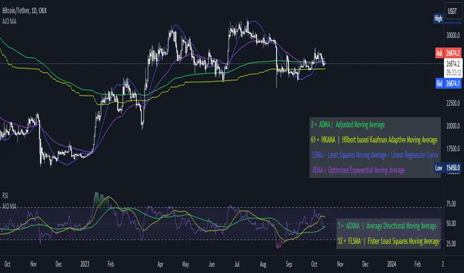
[AIO] Multi Collection Moving Averages 140 MA TypesAll In One Multi Collection Moving Averages.
Since signing up 2 years ago, I have been collecting various Сollections.
I decided to get it into a decent shape and make it one of the biggest collections on TV, and maybe the entire internet.
And now I'm sharing my collection with you.
140 Different Types of Moving Averages are waiting for you.
Specifically :
"
AARMA | Adaptive Autonomous Recursive Moving Average
ADMA | Adjusted Moving Average
ADXMA | Average Directional Moving Average
ADXVMA | Average Directional Volatility Moving Average
AHMA | Ahrens Moving Average
ALF | Ehler Adaptive Laguerre Filter
ALMA | Arnaud Legoux Moving Average
ALSMA | Adaptive Least Squares
ALXMA | Alexander Moving Average
AMA | Adaptive Moving Average
ARI | Unknown
ARSI | Adaptive RSI Moving Average
AUF | Auto Filter
AUTL | Auto-Line
BAMA | Bryant Adaptive Moving Average
BFMA | Blackman Filter Moving Average
CMA | Corrected Moving Average
CORMA | Correlation Moving Average
COVEMA | Coefficient of Variation Weighted Exponential Moving Average
COVNA | Coefficient of Variation Weighted Moving Average
CTI | Coral Trend Indicator
DEC | Ehlers Simple Decycler
DEMA | Double EMA Moving Average
DEVS | Ehlers - Deviation Scaled Moving Average
DONEMA | Donchian Extremum Moving Average
DONMA | Donchian Moving Average
DSEMA | Double Smoothed Exponential Moving Average
DSWF | Damped Sine Wave Weighted Filter
DWMA | Double Weighted Moving Average
E2PBF | Ehlers 2-Pole Butterworth Filter
E2SSF | Ehlers 2-Pole Super Smoother Filter
E3PBF | Ehlers 3-Pole Butterworth Filter
E3SSF | Ehlers 3-Pole Super Smoother Filter
EDMA | Exponentially Deviating Moving Average (MZ EDMA)
EDSMA | Ehlers Dynamic Smoothed Moving Average
EEO | Ehlers Modified Elliptic Filter Optimum
EFRAMA | Ehlers Modified Fractal Adaptive Moving Average
EHMA | Exponential Hull Moving Average
EIT | Ehlers Instantaneous Trendline
ELF | Ehler Laguerre filter
EMA | Exponential Moving Average
EMARSI | EMARSI
EPF | Edge Preserving Filter
EPMA | End Point Moving Average
EREA | Ehlers Reverse Exponential Moving Average
ESSF | Ehlers Super Smoother Filter 2-pole
ETMA | Exponential Triangular Moving Average
EVMA | Elastic Volume Weighted Moving Average
FAMA | Following Adaptive Moving Average
FEMA | Fast Exponential Moving Average
FIBWMA | Fibonacci Weighted Moving Average
FLSMA | Fisher Least Squares Moving Average
FRAMA | Ehlers - Fractal Adaptive Moving Average
FX | Fibonacci X Level
GAUS | Ehlers - Gaussian Filter
GHL | Gann High Low
GMA | Gaussian Moving Average
GMMA | Geometric Mean Moving Average
HCF | Hybrid Convolution Filter
HEMA | Holt Exponential Moving Average
HKAMA | Hilbert based Kaufman Adaptive Moving Average
HMA | Harmonic Moving Average
HSMA | Hirashima Sugita Moving Average
HULL | Hull Moving Average
HULLT | Hull Triple Moving Average
HWMA | Henderson Weighted Moving Average
IE2 | Early T3 by Tim Tilson
IIRF | Infinite Impulse Response Filter
ILRS | Integral of Linear Regression Slope
JMA | Jurik Moving Average
KA | Unknown
KAMA | Kaufman Adaptive Moving Average & Apirine Adaptive MA
KIJUN | KIJUN
KIJUN2 | Kijun v2
LAG | Ehlers - Laguerre Filter
LCLSMA | 1LC-LSMA (1 line code lsma with 3 functions)
LEMA | Leader Exponential Moving Average
LLMA | Low-Lag Moving Average
LMA | Leo Moving Average
LP | Unknown
LRL | Linear Regression Line
LSMA | Least Squares Moving Average / Linear Regression Curve
LTB | Unknown
LWMA | Linear Weighted Moving Average
MAMA | MAMA - MESA Adaptive Moving Average
MAVW | Mavilim Weighted Moving Average
MCGD | McGinley Dynamic Moving Average
MF | Modular Filter
MID | Median Moving Average / Percentile Nearest Rank
MNMA | McNicholl Moving Average
MTMA | Unknown
MVSMA | Minimum Variance SMA
NLMA | Non-lag Moving Average
NWMA | Dürschner 3rd Generation Moving Average (New WMA)
PKF | Parametric Kalman Filter
PWMA | Parabolic Weighted Moving Average
QEMA | Quadruple Exponential Moving Average
QMA | Quick Moving Average
REMA | Regularized Exponential Moving Average
REPMA | Repulsion Moving Average
RGEMA | Range Exponential Moving Average
RMA | Welles Wilders Smoothing Moving Average
RMF | Recursive Median Filter
RMTA | Recursive Moving Trend Average
RSMA | Relative Strength Moving Average - based on RSI
RSRMA | Right Sided Ricker MA
RWMA | Regressively Weighted Moving Average
SAMA | Slope Adaptive Moving Average
SFMA | Smoother Filter Moving Average
SMA | Simple Moving Average
SSB | Senkou Span B
SSF | Ehlers - Super Smoother Filter P2
SSMA | Super Smooth Moving Average
STMA | Unknown
SWMA | Self-Weighted Moving Average
SW_MA | Sine-Weighted Moving Average
TEMA | Triple Exponential Moving Average
THMA | Triple Exponential Hull Moving Average
TL | Unknown
TMA | Triangular Moving Average
TPBF | Three-pole Ehlers Butterworth
TRAMA | Trend Regularity Adaptive Moving Average
TSF | True Strength Force
TT3 | Tilson (3rd Degree) Moving Average
VAMA | Volatility Adjusted Moving Average
VAMAF | Volume Adjusted Moving Average Function
VAR | Vector Autoregression Moving Average
VBMA | Variable Moving Average
VHMA | Vertical Horizontal Moving Average
VIDYA | Variable Index Dynamic Average
VMA | Volume Moving Average
VSO | Unknown
VWMA | Volume Weighted Moving Average
WCD | Unknown
WMA | Weighted Moving Average
XEMA | Optimized Exponential Moving Average
ZEMA | Zero Lag Moving Average
ZLDEMA | Zero-Lag Double Exponential Moving Average
ZLEMA | Ehlers - Zero Lag Exponential Moving Average
ZLTEMA | Zero-Lag Triple Exponential Moving Average
ZSMA | Zero-Lag Simple Moving Average
"
Don't forget that you can use any Moving Average not only for the chart but also for any of your indicators without affecting the code as in my example.
But remember that some MAs are not designed to work with anything other than a chart.
All MA and Code lists are sorted strictly alphabetically by short name (A-Z).
Each MA has its own number (ID) by which you can display the Moving Average you need.
Next to the ID selection there are tooltips with short names and their numbers. Use them.
The panel below will help you to read the Name of the selected MA.
Because of the size of the collection I think this is the optimal and most convenient use. Correct me if this is not the case.
Unknown - Some MAs I collected so long ago that I lost the full real name and couldn't find the authors. If you recognize them, please let me know.
I have deliberately simplified all MAs to input just Source and Length.
Because the collection is so large, it would be quite inconvenient and difficult to customize all MA functions (multipliers, offset, etc.).
If you need or like any MA you will still have to take it from my collection for your code.
I tried to leave the basic MA settings inside function in first strings.
I have tried to list most of the authors, but since the bulk of the collection was created a long time ago and was not intended for public publication I could not find all of them.
Some of the features were created from scratch or may have been slightly modified, so please be careful.
If you would like to improve this collection, please write to me in PM.
Also Credits, Likes, Awards, Loves and Thanks to :
@alexgrover
@allanster
@andre_007
@auroagwei
@blackcat1402
@bsharpe
@cheatcountry
@CrackingCryptocurrency
@Duyck
@ErwinBeckers
@everget
@glaz
@gotbeatz26107
@HPotter
@io72signals
@JacobAmos
@JoshuaMcGowan
@KivancOzbilgic
@LazyBear
@loxx
@LuxAlgo
@MightyZinger
@nemozny
@NGBaltic
@peacefulLizard50262
@RicardoSantos
@StalexBot
@ThiagoSchmitz
@TradingView
— 𝐀𝐧𝐝 𝐎𝐭𝐡𝐞𝐫𝐬 !
So just a Big Thank You to everyone who has ever and anywhere shared their codes.
Cari dalam skrip untuk "harmonic"
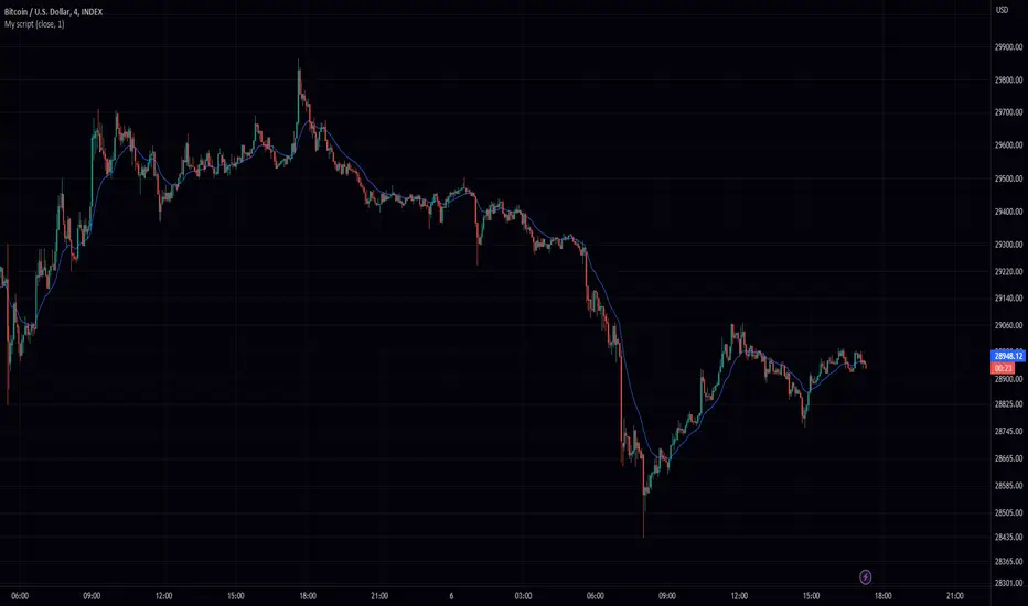
Dominant Period-Based Moving Average (DPBMA)Exploit Market Cycles with the Dominant Period-Based Moving Average Indicator
Introduction:
In the world of trading, market cycles play a crucial role in determining the rhythm of the market. These cycles often consist of recurring patterns that traders can exploit to maximize their profits. One effective way to capitalize on these cycles is by using a moving average (MA) indicator. Today, we are going to introduce you to a unique indicator that takes the most frequent dominant period of the market and uses it as the length of the moving average. This indicator is designed to adapt to the ever-changing market conditions, providing traders with a dynamic tool to better analyze the market.
Dominant Period-Based Moving Average Indicator Overview:
The Dominant Period-Based Moving Average (DPBMA) Indicator is a custom indicator designed to find the most frequent dominant period of the market and use that period as the length of the moving average. This innovative approach allows the indicator to adapt to the market cycles, making it more responsive to the market's changing conditions.
Here's a quick overview of the DPBMA Indicator's features:
Takes the most frequent dominant period of the market.
Uses the dominant period as the length of the moving average.
Adapts to the changing market cycles.
Works as an overlay on your price chart.
Using the Dominant Period-Based Moving Average Indicator:
How the Dominant Period-Based Moving Average Indicator Works:
The DPBMA Indicator works by first importing the DominantCycle function from the lastguru/DominantCycle/2 script. This function calculates the dominant cycle period of the given market data. The DPBMA Indicator then calculates the Exponential Moving Average (EMA) using the dominant period as the length parameter.
The EMA calculation uses an alpha factor, which is calculated as 2 / (length + 1). The alpha factor is then used to smooth the source data (closing prices) and calculate the adaptive moving average.
The DPBMA Indicator also includes a harmonic input, which allows you to multiply the dominant cycle period by an integer value. This can help you fine-tune the indicator to better fit your trading strategy or style.
The Raw Dominant Frequency:
The raw dominant frequency represents the primary cycle period present in the given market data. By identifying the raw dominant frequency, traders can gain insights into the market's current cycle and use this information to make informed trading decisions. The raw dominant frequency can be useful for detecting major trend reversals, support and resistance levels, and potential entry and exit points.
However, using the raw dominant frequency alone has its limitations. For instance, it may not always provide a clear picture of the market's prevailing trend, especially during periods of high market volatility. Additionally, relying solely on the raw dominant frequency may not capture the nuances of shorter-term cycles that can also impact price movements.
The Most Likely Dominant Frequency:
Our approach takes a different angle by focusing on the most likely dominant frequency. This method aims to identify the frequency with the highest probability of being the dominant frequency in the market data. The idea behind this approach is to filter out potential noise and improve the accuracy of the dominant frequency analysis. By using the most likely dominant frequency, traders can gain a more reliable understanding of the market's primary cycle, which can lead to better trading decisions.
In our Dominant Period-Based Moving Average Indicator, we calculate the most likely dominant frequency by analyzing an array of cycle periods and their occurrences in the given market data. We then determine the cycle period with the highest occurrence, representing the most likely dominant frequency. This method allows the indicator to be more adaptive and responsive to the changing market conditions, capturing the nuances of both long-term and short-term cycles.
Why Not the Average Dominant Frequency?
While using the average dominant frequency might seem like a reasonable approach, it can be less effective in accurately capturing the market's primary cycle. Averaging the dominant frequencies may dilute the impact of the true dominant frequency, resulting in a less accurate representation of the market's current cycle. By focusing on the most likely dominant frequency, our approach provides a more accurate and reliable analysis of the market's primary cycle, which can ultimately lead to more effective trading decisions.
Conclusion:
The Dominant Period-Based Moving Average Indicator, enhanced with the most likely dominant frequency approach, offers traders a powerful tool for exploiting market cycles. By adapting to the most frequent dominant period and focusing on the most likely dominant frequency, this indicator provides a more accurate and reliable analysis of the market's primary cycle. As a result, traders can make better-informed decisions, ultimately leading to improved trading performance. Incorporate the DPBMA Indicator into your trading toolbox today, and take advantage of the enhanced market analysis it provides.
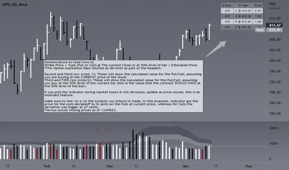
Automated Option Price - Black-Scholes modelPlease make sure you are plotting this indicator on DAILY bars, not doing so will lead to unintended results. Also, make sure that you keep up to date the Risk-free interest rate, which you can consult (for U.S.) on ycharts.com.
This is an indicator that is meant to be used for Options Day Trading, but it can be useful for mid-term or leaps for I also enabled the possibility for user to input manually the Strike and Expiration date. I based the calculation on the Black-Scholes model. Variables included in the calculation are:
-Stock price (S): The current price of the underlying asset (e.g., a stock).
-Strike price (K): The predetermined price at which the option can be exercised.
-Time to expiration (T): The time remaining until the option expires, expressed as a fraction of a year.
-Volatility (σ): The annualized standard deviation of the stock's returns, which is a measure of the stock's price fluctuations.
-Risk-free interest rate (r): The annualized return on a risk-free investment, often approximated by the yield on a government bond.
The only variable I excluded from the original model was the Dividend yield (q).
U S E R I N P U T S:
1. AUTOMATIC calculations enabled:
i) Strike price (K):
Automatically calculate the strike price for both call and put options based on the stock's closing price. The logic follows a set of rules to determine the strike prices which will usually be Out-of-the-Money (OTM):
-If the stock's closing price is between 1 and 60, the call strike price is rounded up to the nearest whole number, while the put strike price is rounded down to the nearest whole number.
-If the stock's closing price is between 60 and 90, the call strike price is rounded up to the nearest whole number and increased by 1, while the put strike price is rounded down to the nearest whole number and decreased by 1.
-If the stock's closing price is between 90 and 120, the call strike price is rounded up to the nearest whole number and increased by 2, while the put strike price is rounded down to the nearest whole number and decreased by 2.
-If the stock's closing price is above 120, the call strike price is rounded up to the nearest multiple of 5, while the put strike price is rounded down to the nearest multiple of 5.
By applying these rules, I just tried to ensure that the automatically calculated strike prices are tailored to the stock's price range, allowing for more accurate option pricing calculations.
ii) Time to expiration (T):
The indicator will consider this week’s expiration contracts (Friday) only when the current day/bar = Monday. If Tuesday or older it will consider the expiration date of the next week’s Friday (because we are not Theta gamblers, right?).
If you are not comfortable with above for whatever reason, you can always…
2. Enter inputs MANUALLY
First make sure you UNTICK the boxes for automatic calculation.
i) Strike price (K) – Self-explanatory
ii) Time to expiration (T) – Just make sure that the horizon you are inputting matches with the next parameter (e.g. you would not input a Monthly risk-free interest rate for a Leap).
iii) Risk-free interest rate (r) – You can pull this data from the web. Here’s the link I used to define the value that this indicator was launched with:
ycharts.com
Don’t get obsessed with updating this daily if you are using this for day trading, you will notice that weekly may be more than enough.
V O L A T I L I T Y
Not option to manually input Volatility so I’ll explain how it is calculated in this script:
I considered two measures of volatility; one is derived calculating the annualized volatility using the standard deviation of daily returns and the second one is the ATR-based annualized volatility. I then used a ‘combined’ approach with the harmonic mean and the arithmetic mean of these results which can help account for the variability in the option prices calculated with different volatility estimates, which can be more robust when dealing with outliers or skewed data. I back tested with some samples of actual option prices and found that this approach is the one that got results closer to the actual bids.
T A B L E
Nomenclature to read rows is:
Option Strike Price | Type of Option (Put or Call) @ The current Close or at 50% level of bar | Estimated Price
*The Option expiration Date showed as dd-MMM as part of the headers.
Second and third row (color 1): These will show the calculated value for the Put/Call, assuming you are buying at the CURRENT price of the stock.
Third and Fifth row (color2): These will show the calculated value for the Put/Call, assuming you buy at the 50% level of the current bar (this is the value that the contract WOULD HAVE at the 50% level of the bar).
If you plot the indicator during market hours it will obviously update as price moves, this is an intended feature.
L I M I T A T I O N S
The Black-Scholes model, like many other models, has its limitations and will oftentimes provide inaccurate option prices in all market conditions. High volatility events, such as earnings announcements, can lead to significant price fluctuations that are not fully captured by the model.
The model assumes that the stock price follows a continuous random walk with constant volatility, but in reality, volatility can change over time, and stock prices can exhibit jumps, especially around significant events like earnings announcements. This can cause the model to underestimate the true option price in such situations.
Please make sure that you first back test on the symbols you trade to ensure the information presented by this indicator will suit your trading strategy. You will find that the delta between the proposed price of the indicator versus the actual price may differ significantly in some symbols while for others it will be very close. For instance, today (13APR23), the prices for AMD, DIS, AAPL (puts only), were very close to actual bids, whereas TSLA differ significantly (but then again, take a look at the calendar and this last symbol is having earnings next week which may add a premium to the contracts)… I am sure you will get your own conclusions and applicable use cases based on the data you test with.
As always, be wise and methodical on the investment or trading decisions you make!
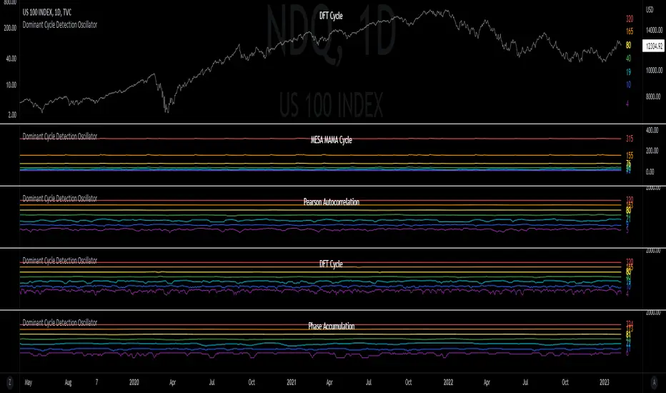
Dominant Cycle Detection OscillatorThis is a Dominant Cycle Detection Oscillator that searches multiple ranges of wavelengths within a spectrum. Choose one of 4 different dominant cycle detection methods (MESA MAMA cycle, Pearson Autocorrelation, Discreet Fourier Transform, and Phase Accumulation) to determine the most dominant cycles and see the historical results. Straight lines can indicate a steady dominant cycle; while Wavy lines might indicate a varying dominant cycle length. The steadier the cycle, the easier it may be to predict future events in that cycle (keep the log scale in mind when considering steadiness). The presence of evenly divisible (or harmonic) cycle lengths may also indicate stronger cycles; for example, 19, 38, and 76 dominant lengths for the 2x, 4x, and 8x cycles. Practically, a trader can use these cycle outputs as the default settings for other Hurst/cycle indicators. For example, if you see dominant cycle oscillator outputs of 38 & 76 for the 4x and 8x cycle respectively, you might want to test/use defaults of 38 & 76 for the 4x & 8x lengths in the bandpass, diamond/semi-circle notation, moving average & envelope, and FLD instead of the defaults 40 & 80 for a more fine-tuned analysis.
Muting the oscillator's historical lines and overlaying the indicator on the chart can visually cue a trader to the cycle lengths without taking up extra panes. The DFT Cycle lengths with muted historical lines have been overlayed on the chart in the photo.
The y-axis scale for this indicator's pane (just the oscillator pane, not the chart) most likely needs to be changed to logarithmic to look normal, but it depends on the search ranges in your settings. There are instructions in the settings. In the photo, the MESA MAMA scale is set to regular (not logarithmic) which demonstrates how difficult it can be to read if not changed.
In the Spectral Analysis chapter of Hurst's book Profit Magic, he recommended doing a Fourier analysis across a spectrum of frequencies. Hurst acknowledged there were many ways to do this analysis but recommended the method described by Lanczos. Currently in this indicator, the closest thing to the method described by Lanczos is the DFT Discreet Fourier Transform method.
Shoutout to @lastguru for the dominant cycle library referenced in this code. He mentioned that he may add more methods in the future.
Channel Based Zigzag [HeWhoMustNotBeNamed]🎲 Concept
Zigzag is built based on the price and number of offset bars. But, in this experiment, we build zigzag based on different bands such as Bollinger Band, Keltner Channel and Donchian Channel. The process is simple:
🎯 Derive bands based on input parameters
🎯 High of a bar is considered as pivot high only if the high price is above or equal to upper band.
🎯 Similarly low of a bar is considered as pivot low only if low price is below or equal to lower band.
🎯 Adding the pivot high/low follows same logic as that of regular zigzag where pivot high is always followed by pivot low and vice versa.
🎯 If the new pivot added is of same direction as that of last pivot, then both pivots are compared with each other and only the extreme one is kept. (Highest in case of pivot high and lowest in case of pivot low)
🎯 If a bar has both pivot high and pivot low - pivot with same direction as previous pivot is added to the list first before adding the pivot with opposite direction.
🎲 Use Cases
Can be used for pattern recognition algorithms instead of standard zigzag. This will help derive patterns which are relative to bands and channels.
Example: John Bollinger explains how to manually scan double tap using Bollinger Bands in this video: www.youtube.com This modified zigzag base can be used to achieve the same using algorithmic means.
🎲 Settings
Few simple configurations which will let you select the band properties. Notice that there is no zigzag length here. All the calculations depend on the bands.
With bands display, indicator looks something like this
Note that pivots do not always represent highest/lowest prices. They represent highest/lowest price relative to bands.
As mentioned many times, application of zigzag is not for buying at lower price and selling at higher price. It is mainly used for pattern recognition either manually or via algorithms. Lets build new Harmonic, Chart patterns, Trend Lines using the new zigzag?

Musashi_Katana=== Musashi-Katana ===
This tool was designed to fit my particular trading style and personal theories about the "Alchemy of the markets" and ''Harmonic Structure'.
Context
When following a Technical approach to to surf the markets, there are teachings that must be understood before reaching a confort-zone, this usually happen the possible worst way by constant experimentation, it hurts.
Here few technical hints:
- Align High timeframes with lower timeframes:
This simple concept relax a lot complexity of finding of a trend bias. Musashi-Katana allows you to use technical indicator corresponding to specific timeframes, like daily weekly or yearly. They wont change when you change the chart's timeframe, its very useful as you know where you're standing in the long term, Its quite relaxing.
- Use volume:
The constant usage of volume will allow you to sync with the market's breathing. This shows you the mass of money flowing into and out of the market, is key if you want to understand momentum. This tool can help here, as it have multi-period vwaps. You can use yearly, monthly for swing trading, and even weekly if you enjoy scalping.
Useful stuff:
- You have access to baselines, AMA and Kijun-sen with the possibility of adding ATR bands.
- AMAs come as two lines strategies for different approaches, fast medium or slow.
- You can experiment with normal and multi timeframe moving averages and other trend tools.
Final Note
If used correctly Musashi-Katana is a very powerful tool, which makes no sense as there is no correct usage. Don't add everything at the same time, experiment, combine stuff, every market is different.
Backtest every possible strategy before using it, see what works and doesn't. This gives you a lot of peace, specially while you're at the tip of the spear surfing the markets
--> I personally use this in combination with 'Musashi_Slasher (Mometum+Volatility)', as it gives me volatility and momentum in a very precise way.

QQE Student's T-Distribution Bollinger Bands Oscillator Credit to all of the developers on this project (aka all of the places I got the code from lol) @eylwithsteph @storma @Fractured @lejmer @AlexGrover @Montyjus @Jiehonglim @StephXAGs @peacefulLizard50262 @gorx1 @above-c-level
This script utilizes @above-c-level 's Student's T-Distribution script to give us a great estimation of volatility. I took this idea and apply it to the QQE filter! That being said I have added a boat load of features as to make this script as useful to as many people as possible. This is the Osc version
Included averages: 'TMA', 'ALMA', 'EMA', 'DEMA', 'TEMA', 'WMA', 'VWMA', 'SMA', 'SMMA', 'HMA', 'LSMA', 'JMA', 'VAMA', 'FRAMA', 'ZLEMA', 'KAMA', 'IDWMA', 'FLMSA', 'PEMA', 'HCF', 'TIF', 'MF', 'ARMA', 'DAF', 'WRMA', 'RMA', 'RAF', 'A2RMA', 'QQE 1', 'QQE 2','Centroid',"Harmonic Mean","Geometric Mean","Quadratic Mean","Median","Trimean","Midhinge","Midrange","VWAP"
Included Features: Smoothing, Additional Moving Average, Log Space, Mean Momentum via Derivative, Normalization, Convergence DIvergence, Candle View
Use this just like macd/rsi but instead this directly reflects the band version! It also shows really valid support and resistance. Use this in combination with the band version for more power.

QQE Student's T-Distribution Bollinger BandsCredit to all of the developers on this project (aka all of the places I got the code from lol) @eylwithsteph @storma @Fractured @lejmer @AlexGrover @Montyjus @Jiehonglim @StephXAGs @peacefulLizard50262 @gorx1 @above-c-level
This script utilizes @above-c-level 's Student's T-Distribution script to give us a great estimation of volatility. I took this idea and apply it to the QQE filter! That being said I have added a boat load of features as to make this script as useful to as many people as possible.
Included averages: 'TMA', 'ALMA', 'EMA', 'DEMA', 'TEMA', 'WMA', 'VWMA', 'SMA', 'SMMA', 'HMA', 'LSMA', 'JMA', 'VAMA', 'FRAMA', 'ZLEMA', 'KAMA', 'IDWMA', 'FLMSA', 'PEMA', 'HCF', 'TIF', 'MF', 'ARMA', 'DAF', 'WRMA', 'RMA', 'RAF', 'A2RMA', 'QQE 1', 'QQE 2','Centroid',"Harmonic Mean","Geometric Mean","Quadratic Mean","Median","Trimean","Midhinge","Midrange","VWAP"
Included Features: Smoothing, Additional Moving Average, Log Space, Mean Momentum via Derivative
Use this just like BB but instead (as long as you are on qqe) you get real prices that are stable! It also shows really valid support and resistance. Use this in combination with the osc version for more power.
HH-LL ZZAnother ZigZag, yes...
I believe though this concerns another angle/principle, therefore I wanted to share
How does it work?
Given:
source for level breach -> close
X breaches -> 3
Let's say this is the latest found 'lower low' (LL - blue dot under bar):
This bar has been triggered because 3 bars closed under low of previous 'trigger bar' (TB )
The high and low of this new TB will act as triggers
(aqua blue lines, seen in image above)
Then there are 2 options:
- again 3 bars closes under the latest TB , in that case the TB moves to that new LL.
- 3 bars closes higher than the high of previous TB
The high and low of this new TB act again as trigger
If a new TB LL/HH is found, the script checks previous LL/HH
and searches the highest/lowest point in between.
If necessary, the temporary highest/lowest will be adjusted:
Another example:
The last 2 points can change (repaint).
Yellow coloured lines/labels are set and won't change anymore.
Concluded:
In case of these settings:
source for level breach -> close
X breaches -> 3
once a new TB is found, the high and low act as trigger lines
- when 3 bars closes under that low , a new LL is found, this will be the new TB
- when 3 bars closes above that high , a new HH is found, this will be the new TB
and so on...
Settings:
source for level breach -> close or high/low - H/L
X breaches -> 1 -> 10
line style -> solid, dotted, dashed
show level breaches -> new found TB (blue/lime coloured)
show Support/Resistance (lines at the right)
repaint warning can be removed
show labels / lines
This ZZ can be used for Harmonic patterns, Trend evaluation, support/resistance,...
In this script, I also used new features
- text_font_family = font.family_monospace -> link
- display=display.pane -> link
Cheers!
STD/Clutter-Filtered, Variety FIR Filters [Loxx]STD/Clutter-Filtered, Variety FIR Filters is a FIR filter explorer. The following FIR Digital Filters are included.
Rectangular - simple moving average
Hanning
Hamming
Blackman
Blackman/Harris
Linear weighted
Triangular
There are 10s of windowing functions like the ones listed above. This indicator will be updated over time as I create more windowing functions in Pine.
Uniform/Rectangular Window
The uniform window (also called the rectangular window) is a time window with unity amplitude for all time samples and has the same effect as not applying a window.
Use this window when leakage is not a concern, such as observing an entire transient signal.
The uniform window has a rectangular shape and does not attenuate any portion of the time record. It weights all parts of the time record equally. Because the uniform window does not force the signal to appear periodic in the time record, it is generally used only with functions that are already periodic within a time record, such as transients and bursts.
The uniform window is sometimes called a transient or boxcar window.
For sine waves that are exactly periodic within a time record, using the uniform window allows you to measure the amplitude exactly (to within hardware specifications) from the Spectrum trace.
Hanning Window
The Hanning window attenuates the input signal at both ends of the time record to zero. This forces the signal to appear periodic. The Hanning window offers good frequency resolution at the expense of some amplitude accuracy.
This window is typically used for broadband signals such as random noise. This window should not be used for burst or chirp source types or other strictly periodic signals. The Hanning window is sometimes called the Hann window or random window.
Hamming Window
Computers can't do computations with an infinite number of data points, so all signals are "cut off" at either end. This causes the ripple on either side of the peak that you see. The hamming window reduces this ripple, giving you a more accurate idea of the original signal's frequency spectrum.
Blackman
The Blackman window is a taper formed by using the first three terms of a summation of cosines. It was designed to have close to the minimal leakage possible. It is close to optimal, only slightly worse than a Kaiser window.
Blackman-Harris
This is the original "Minimum 4-sample Blackman-Harris" window, as given in the classic window paper by Fredric Harris "On the Use of Windows for Harmonic Analysis with the Discrete Fourier Transform", Proceedings of the IEEE, vol 66, no. 1, pp. 51-83, January 1978. The maximum side-lobe level is -92.00974072 dB.
Linear Weighted
A Weighted Moving Average puts more weight on recent data and less on past data. This is done by multiplying each bar’s price by a weighting factor. Because of its unique calculation, WMA will follow prices more closely than a corresponding Simple Moving Average.
Triangular Weighted
Triangular windowing is known for very smooth results. The weights in the triangular moving average are adding more weight to central values of the averaged data. Hence the coefficients are specifically distributed. Some of the examples that can give a clear picture of the coefficients progression:
period 1 : 1
period 2 : 1 1
period 3 : 1 2 1
period 4 : 1 2 2 1
period 5 : 1 2 3 2 1
period 6 : 1 2 3 3 2 1
period 7 : 1 2 3 4 3 2 1
period 8 : 1 2 3 4 4 3 2 1
Read here to read about how each of these filters compare with each other: Windowing
What is a Finite Impulse Response Filter?
In signal processing, a finite impulse response (FIR) filter is a filter whose impulse response (or response to any finite length input) is of finite duration, because it settles to zero in finite time. This is in contrast to infinite impulse response (IIR) filters, which may have internal feedback and may continue to respond indefinitely (usually decaying).
The impulse response (that is, the output in response to a Kronecker delta input) of an Nth-order discrete-time FIR filter lasts exactly {\displaystyle N+1}N+1 samples (from first nonzero element through last nonzero element) before it then settles to zero.
FIR filters can be discrete-time or continuous-time, and digital or analog.
A FIR filter is (similar to, or) just a weighted moving average filter, where (unlike a typical equally weighted moving average filter) the weights of each delay tap are not constrained to be identical or even of the same sign. By changing various values in the array of weights (the impulse response, or time shifted and sampled version of the same), the frequency response of a FIR filter can be completely changed.
An FIR filter simply CONVOLVES the input time series (price data) with its IMPULSE RESPONSE. The impulse response is just a set of weights (or "coefficients") that multiply each data point. Then you just add up all the products and divide by the sum of the weights and that is it; e.g., for a 10-bar SMA you just add up 10 bars of price data (each multiplied by 1) and divide by 10. For a weighted-MA you add up the product of the price data with triangular-number weights and divide by the total weight.
Ultra Low Lag Moving Average's weights are designed to have MAXIMUM possible smoothing and MINIMUM possible lag compatible with as-flat-as-possible phase response.
What is a Clutter Filter?
For our purposes here, this is a filter that compares the slope of the trading filter output to a threshold to determine whether to shift trends. If the slope is up but the slope doesn't exceed the threshold, then the color is gray and this indicates a chop zone. If the slope is down but the slope doesn't exceed the threshold, then the color is gray and this indicates a chop zone. Alternatively if either up or down slope exceeds the threshold then the trend turns green for up and red for down. Fro demonstration purposes, an EMA is used as the moving average. This acts to reduce the noise in the signal.
Included
Bar coloring
Loxx's Expanded Source Types
Signals
Alerts
Related Indicators
STD/Clutter-Filtered, Kaiser Window FIR Digital Filter
STD- and Clutter-Filtered, Non-Lag Moving Average
Clutter-Filtered, D-Lag Reducer, Spec. Ops FIR Filter
STD-Filtered, Ultra Low Lag Moving Average

Normalized, Variety, Fast Fourier Transform Explorer [Loxx]Normalized, Variety, Fast Fourier Transform Explorer demonstrates Real, Cosine, and Sine Fast Fourier Transform algorithms. This indicator can be used as a rule of thumb but shouldn't be used in trading.
What is the Discrete Fourier Transform?
In mathematics, the discrete Fourier transform (DFT) converts a finite sequence of equally-spaced samples of a function into a same-length sequence of equally-spaced samples of the discrete-time Fourier transform (DTFT), which is a complex-valued function of frequency. The interval at which the DTFT is sampled is the reciprocal of the duration of the input sequence. An inverse DFT is a Fourier series, using the DTFT samples as coefficients of complex sinusoids at the corresponding DTFT frequencies. It has the same sample-values as the original input sequence. The DFT is therefore said to be a frequency domain representation of the original input sequence. If the original sequence spans all the non-zero values of a function, its DTFT is continuous (and periodic), and the DFT provides discrete samples of one cycle. If the original sequence is one cycle of a periodic function, the DFT provides all the non-zero values of one DTFT cycle.
What is the Complex Fast Fourier Transform?
The complex Fast Fourier Transform algorithm transforms N real or complex numbers into another N complex numbers. The complex FFT transforms a real or complex signal x in the time domain into a complex two-sided spectrum X in the frequency domain. You must remember that zero frequency corresponds to n = 0, positive frequencies 0 < f < f_c correspond to values 1 ≤ n ≤ N/2 −1, while negative frequencies −fc < f < 0 correspond to N/2 +1 ≤ n ≤ N −1. The value n = N/2 corresponds to both f = f_c and f = −f_c. f_c is the critical or Nyquist frequency with f_c = 1/(2*T) or half the sampling frequency. The first harmonic X corresponds to the frequency 1/(N*T).
The complex FFT requires the list of values (resolution, or N) to be a power 2. If the input size if not a power of 2, then the input data will be padded with zeros to fit the size of the closest power of 2 upward.
What is Real-Fast Fourier Transform?
Has conditions similar to the complex Fast Fourier Transform value, except that the input data must be purely real. If the time series data has the basic type complex64, only the real parts of the complex numbers are used for the calculation. The imaginary parts are silently discarded.
What is the Real-Fast Fourier Transform?
In many applications, the input data for the DFT are purely real, in which case the outputs satisfy the symmetry
X(N-k)=X(k)
and efficient FFT algorithms have been designed for this situation (see e.g. Sorensen, 1987). One approach consists of taking an ordinary algorithm (e.g. Cooley–Tukey) and removing the redundant parts of the computation, saving roughly a factor of two in time and memory. Alternatively, it is possible to express an even-length real-input DFT as a complex DFT of half the length (whose real and imaginary parts are the even/odd elements of the original real data), followed by O(N) post-processing operations.
It was once believed that real-input DFTs could be more efficiently computed by means of the discrete Hartley transform (DHT), but it was subsequently argued that a specialized real-input DFT algorithm (FFT) can typically be found that requires fewer operations than the corresponding DHT algorithm (FHT) for the same number of inputs. Bruun's algorithm (above) is another method that was initially proposed to take advantage of real inputs, but it has not proved popular.
There are further FFT specializations for the cases of real data that have even/odd symmetry, in which case one can gain another factor of roughly two in time and memory and the DFT becomes the discrete cosine/sine transform(s) (DCT/DST). Instead of directly modifying an FFT algorithm for these cases, DCTs/DSTs can also be computed via FFTs of real data combined with O(N) pre- and post-processing.
What is the Discrete Cosine Transform?
A discrete cosine transform ( DCT ) expresses a finite sequence of data points in terms of a sum of cosine functions oscillating at different frequencies. The DCT , first proposed by Nasir Ahmed in 1972, is a widely used transformation technique in signal processing and data compression. It is used in most digital media, including digital images (such as JPEG and HEIF, where small high-frequency components can be discarded), digital video (such as MPEG and H.26x), digital audio (such as Dolby Digital, MP3 and AAC ), digital television (such as SDTV, HDTV and VOD ), digital radio (such as AAC+ and DAB+), and speech coding (such as AAC-LD, Siren and Opus). DCTs are also important to numerous other applications in science and engineering, such as digital signal processing, telecommunication devices, reducing network bandwidth usage, and spectral methods for the numerical solution of partial differential equations.
The use of cosine rather than sine functions is critical for compression, since it turns out (as described below) that fewer cosine functions are needed to approximate a typical signal, whereas for differential equations the cosines express a particular choice of boundary conditions. In particular, a DCT is a Fourier-related transform similar to the discrete Fourier transform (DFT), but using only real numbers. The DCTs are generally related to Fourier Series coefficients of a periodically and symmetrically extended sequence whereas DFTs are related to Fourier Series coefficients of only periodically extended sequences. DCTs are equivalent to DFTs of roughly twice the length, operating on real data with even symmetry (since the Fourier transform of a real and even function is real and even), whereas in some variants the input and/or output data are shifted by half a sample. There are eight standard DCT variants, of which four are common.
The most common variant of discrete cosine transform is the type-II DCT , which is often called simply "the DCT". This was the original DCT as first proposed by Ahmed. Its inverse, the type-III DCT , is correspondingly often called simply "the inverse DCT" or "the IDCT". Two related transforms are the discrete sine transform ( DST ), which is equivalent to a DFT of real and odd functions, and the modified discrete cosine transform (MDCT), which is based on a DCT of overlapping data. Multidimensional DCTs ( MD DCTs) are developed to extend the concept of DCT to MD signals. There are several algorithms to compute MD DCT . A variety of fast algorithms have been developed to reduce the computational complexity of implementing DCT . One of these is the integer DCT (IntDCT), an integer approximation of the standard DCT ,: ix, xiii, 1, 141–304 used in several ISO /IEC and ITU-T international standards.
What is the Discrete Sine Transform?
In mathematics, the discrete sine transform (DST) is a Fourier-related transform similar to the discrete Fourier transform (DFT), but using a purely real matrix. It is equivalent to the imaginary parts of a DFT of roughly twice the length, operating on real data with odd symmetry (since the Fourier transform of a real and odd function is imaginary and odd), where in some variants the input and/or output data are shifted by half a sample.
A family of transforms composed of sine and sine hyperbolic functions exists. These transforms are made based on the natural vibration of thin square plates with different boundary conditions.
The DST is related to the discrete cosine transform (DCT), which is equivalent to a DFT of real and even functions. See the DCT article for a general discussion of how the boundary conditions relate the various DCT and DST types. Generally, the DST is derived from the DCT by replacing the Neumann condition at x=0 with a Dirichlet condition. Both the DCT and the DST were described by Nasir Ahmed T. Natarajan and K.R. Rao in 1974. The type-I DST (DST-I) was later described by Anil K. Jain in 1976, and the type-II DST (DST-II) was then described by H.B. Kekra and J.K. Solanka in 1978.
Notable settings
windowper = period for calculation, restricted to powers of 2: "16", "32", "64", "128", "256", "512", "1024", "2048", this reason for this is FFT is an algorithm that computes DFT (Discrete Fourier Transform) in a fast way, generally in 𝑂(𝑁⋅log2(𝑁)) instead of 𝑂(𝑁2). To achieve this the input matrix has to be a power of 2 but many FFT algorithm can handle any size of input since the matrix can be zero-padded. For our purposes here, we stick to powers of 2 to keep this fast and neat. read more about this here: Cooley–Tukey FFT algorithm
SS = smoothing count, this smoothing happens after the first FCT regular pass. this zeros out frequencies from the previously calculated values above SS count. the lower this number, the smoother the output, it works opposite from other smoothing periods
Fmin1 = zeroes out frequencies not passing this test for min value
Fmax1 = zeroes out frequencies not passing this test for max value
barsback = moves the window backward
Inverse = whether or not you wish to invert the FFT after first pass calculation
Related indicators
Real-Fast Fourier Transform of Price Oscillator
STD-Stepped Fast Cosine Transform Moving Average
Real-Fast Fourier Transform of Price w/ Linear Regression
Variety RSI of Fast Discrete Cosine Transform
Additional reading
A Fast Computational Algorithm for the Discrete Cosine Transform by Chen et al.
Practical Fast 1-D DCT Algorithms With 11 Multiplications by Loeffler et al.
Cooley–Tukey FFT algorithm
Ahmed, Nasir (January 1991). "How I Came Up With the Discrete Cosine Transform". Digital Signal Processing. 1 (1): 4–5. doi:10.1016/1051-2004(91)90086-Z.
DCT-History - How I Came Up With The Discrete Cosine Transform
Comparative Analysis for Discrete Sine Transform as a suitable method for noise estimation

Real-Fast Fourier Transform of Price Oscillator [Loxx]Real-Fast Fourier Transform Oscillator is a simple Real-Fast Fourier Transform Oscillator. You have the option to turn on inverse filter as well as min/max filters to fine tune the oscillator. This oscillator is normalized by default. This indicator is to demonstrate how one can easily turn the RFFT algorithm into an oscillator..
What is the Discrete Fourier Transform?
In mathematics, the discrete Fourier transform (DFT) converts a finite sequence of equally-spaced samples of a function into a same-length sequence of equally-spaced samples of the discrete-time Fourier transform (DTFT), which is a complex-valued function of frequency. The interval at which the DTFT is sampled is the reciprocal of the duration of the input sequence. An inverse DFT is a Fourier series, using the DTFT samples as coefficients of complex sinusoids at the corresponding DTFT frequencies. It has the same sample-values as the original input sequence. The DFT is therefore said to be a frequency domain representation of the original input sequence. If the original sequence spans all the non-zero values of a function, its DTFT is continuous (and periodic), and the DFT provides discrete samples of one cycle. If the original sequence is one cycle of a periodic function, the DFT provides all the non-zero values of one DTFT cycle.
What is the Complex Fast Fourier Transform?
The complex Fast Fourier Transform algorithm transforms N real or complex numbers into another N complex numbers. The complex FFT transforms a real or complex signal x in the time domain into a complex two-sided spectrum X in the frequency domain. You must remember that zero frequency corresponds to n = 0, positive frequencies 0 < f < f_c correspond to values 1 ≤ n ≤ N/2 −1, while negative frequencies −fc < f < 0 correspond to N/2 +1 ≤ n ≤ N −1. The value n = N/2 corresponds to both f = f_c and f = −f_c. f_c is the critical or Nyquist frequency with f_c = 1/(2*T) or half the sampling frequency. The first harmonic X corresponds to the frequency 1/(N*T).
The complex FFT requires the list of values (resolution, or N) to be a power 2. If the input size if not a power of 2, then the input data will be padded with zeros to fit the size of the closest power of 2 upward.
What is Real-Fast Fourier Transform?
Has conditions similar to the complex Fast Fourier Transform value, except that the input data must be purely real. If the time series data has the basic type complex64, only the real parts of the complex numbers are used for the calculation. The imaginary parts are silently discarded.
Included
Moving window from Last Bar setting. You can lock the oscillator in place on the current bar by adding 1 every time a new bar appears in the Last Bar Setting

Real-Fast Fourier Transform of Price w/ Linear Regression [Loxx]Real-Fast Fourier Transform of Price w/ Linear Regression is a indicator that implements a Real-Fast Fourier Transform on Price and modifies the output by a measure of Linear Regression. The solid line is the Linear Regression Trend of the windowed data, The green/red line is the Real FFT of price.
What is the Discrete Fourier Transform?
In mathematics, the discrete Fourier transform (DFT) converts a finite sequence of equally-spaced samples of a function into a same-length sequence of equally-spaced samples of the discrete-time Fourier transform (DTFT), which is a complex-valued function of frequency. The interval at which the DTFT is sampled is the reciprocal of the duration of the input sequence. An inverse DFT is a Fourier series, using the DTFT samples as coefficients of complex sinusoids at the corresponding DTFT frequencies. It has the same sample-values as the original input sequence. The DFT is therefore said to be a frequency domain representation of the original input sequence. If the original sequence spans all the non-zero values of a function, its DTFT is continuous (and periodic), and the DFT provides discrete samples of one cycle. If the original sequence is one cycle of a periodic function, the DFT provides all the non-zero values of one DTFT cycle.
What is the Complex Fast Fourier Transform?
The complex Fast Fourier Transform algorithm transforms N real or complex numbers into another N complex numbers. The complex FFT transforms a real or complex signal x in the time domain into a complex two-sided spectrum X in the frequency domain. You must remember that zero frequency corresponds to n = 0, positive frequencies 0 < f < f_c correspond to values 1 ≤ n ≤ N/2 −1, while negative frequencies −fc < f < 0 correspond to N/2 +1 ≤ n ≤ N −1. The value n = N/2 corresponds to both f = f_c and f = −f_c. f_c is the critical or Nyquist frequency with f_c = 1/(2*T) or half the sampling frequency. The first harmonic X corresponds to the frequency 1/(N*T).
The complex FFT requires the list of values (resolution, or N) to be a power 2. If the input size if not a power of 2, then the input data will be padded with zeros to fit the size of the closest power of 2 upward.
What is Real-Fast Fourier Transform?
Has conditions similar to the complex Fast Fourier Transform value, except that the input data must be purely real. If the time series data has the basic type complex64, only the real parts of the complex numbers are used for the calculation. The imaginary parts are silently discarded.
Inputs:
src = source price
uselreg = whether you wish to modify output with linear regression calculation
Windowin = windowing period, restricted to powers of 2: "4", "8", "16", "32", "64", "128", "256", "512", "1024", "2048"
Treshold = to modified power output to fine tune signal
dtrendper = adjust regression calculation
barsback = move window backward from bar 0
mutebars = mute bar coloring for the range
Further reading:
Real-valued Fast Fourier Transform Algorithms IEEE Transactions on Acoustics, Speech, and Signal Processing, June 1987
Related indicators utilizing Fourier Transform
Fourier Extrapolator of Variety RSI w/ Bollinger Bands
Fourier Extrapolation of Variety Moving Averages
Fourier Extrapolator of Price w/ Projection Forecast

Dynamic Zone Range on OMA [Loxx]Dynamic Zone Range on OMA is an One More Moving Average oscillator with Dynamic Zones.
What is the One More Moving Average (OMA)?
The usual story goes something like this : which is the best moving average? Everyone that ever started to do any kind of technical analysis was pulled into this "game". Comparing, testing, looking for new ones, testing ...
The idea of this one is simple: it should not be itself, but it should be a kind of a chameleon - it should "imitate" as much other moving averages as it can. So the need for zillion different moving averages would diminish. And it should have some extra, of course:
The extras:
it has to be smooth
it has to be able to "change speed" without length change
it has to be able to adapt or not (since it has to "imitate" the non-adaptive as well as the adaptive ones)
The steps:
Smoothing - compared are the simple moving average (that is the basis and the first step of this indicator - a smoothed simple moving average with as little lag added as it is possible and as close to the original as it is possible) Speed 1 and non-adaptive are the reference for this basic setup.
Speed changing - same chart only added one more average with "speeds" 2 and 3 (for comparison purposes only here)
Finally - adapting : same chart with SMA compared to one more average with speed 1 but adaptive (so this parameters would make it a "smoothed adaptive simple average") Adapting part is a modified Kaufman adapting way and this part (the adapting part) may be a subject for changes in the future (it is giving satisfactory results, but if or when I find a better way, it will be implemented here)
Some comparisons for different speed settings (all the comparisons are without adaptive turned on, and are approximate. Approximation comes from a fact that it is impossible to get exactly the same values from only one way of calculation, and frankly, I even did not try to get those same values).
speed 0.5 - T3 (0.618 Tilson)
speed 2.5 - T3 (0.618 Fulks/Matulich)
speed 1 - SMA , harmonic mean
speed 2 - LWMA
speed 7 - very similar to Hull and TEMA
speed 8 - very similar to LSMA and Linear regression value
Parameters:
Length - length (period) for averaging
Source - price to use for averaging
Speed - desired speed (i limited to -1.5 on the lower side but it even does not need that limit - some interesting results with speeds that are less than 0 can be achieved)
Adaptive - does it adapt or not
Variety Moving Averages w/ Dynamic Zones contains 33 source types and 35+ moving averages with double dynamic zones levels.
What are Dynamic Zones?
As explained in "Stocks & Commodities V15:7 (306-310): Dynamic Zones by Leo Zamansky, Ph .D., and David Stendahl"
Most indicators use a fixed zone for buy and sell signals. Here’ s a concept based on zones that are responsive to past levels of the indicator.
One approach to active investing employs the use of oscillators to exploit tradable market trends. This investing style follows a very simple form of logic: Enter the market only when an oscillator has moved far above or below traditional trading lev- els. However, these oscillator- driven systems lack the ability to evolve with the market because they use fixed buy and sell zones. Traders typically use one set of buy and sell zones for a bull market and substantially different zones for a bear market. And therein lies the problem.
Once traders begin introducing their market opinions into trading equations, by changing the zones, they negate the system’s mechanical nature. The objective is to have a system automatically define its own buy and sell zones and thereby profitably trade in any market — bull or bear. Dynamic zones offer a solution to the problem of fixed buy and sell zones for any oscillator-driven system.
An indicator’s extreme levels can be quantified using statistical methods. These extreme levels are calculated for a certain period and serve as the buy and sell zones for a trading system. The repetition of this statistical process for every value of the indicator creates values that become the dynamic zones. The zones are calculated in such a way that the probability of the indicator value rising above, or falling below, the dynamic zones is equal to a given probability input set by the trader.
To better understand dynamic zones, let's first describe them mathematically and then explain their use. The dynamic zones definition:
Find V such that:
For dynamic zone buy: P{X <= V}=P1
For dynamic zone sell: P{X >= V}=P2
where P1 and P2 are the probabilities set by the trader, X is the value of the indicator for the selected period and V represents the value of the dynamic zone.
The probability input P1 and P2 can be adjusted by the trader to encompass as much or as little data as the trader would like. The smaller the probability, the fewer data values above and below the dynamic zones. This translates into a wider range between the buy and sell zones. If a 10% probability is used for P1 and P2, only those data values that make up the top 10% and bottom 10% for an indicator are used in the construction of the zones. Of the values, 80% will fall between the two extreme levels. Because dynamic zone levels are penetrated so infrequently, when this happens, traders know that the market has truly moved into overbought or oversold territory.
Calculating the Dynamic Zones
The algorithm for the dynamic zones is a series of steps. First, decide the value of the lookback period t. Next, decide the value of the probability Pbuy for buy zone and value of the probability Psell for the sell zone.
For i=1, to the last lookback period, build the distribution f(x) of the price during the lookback period i. Then find the value Vi1 such that the probability of the price less than or equal to Vi1 during the lookback period i is equal to Pbuy. Find the value Vi2 such that the probability of the price greater or equal to Vi2 during the lookback period i is equal to Psell. The sequence of Vi1 for all periods gives the buy zone. The sequence of Vi2 for all periods gives the sell zone.
In the algorithm description, we have: Build the distribution f(x) of the price during the lookback period i. The distribution here is empirical namely, how many times a given value of x appeared during the lookback period. The problem is to find such x that the probability of a price being greater or equal to x will be equal to a probability selected by the user. Probability is the area under the distribution curve. The task is to find such value of x that the area under the distribution curve to the right of x will be equal to the probability selected by the user. That x is the dynamic zone.
Included
4 signal types
Bar coloring
Alerts
Channels fill
Pips-Stepped, OMA-Filtered, Ocean NMA [Loxx]Pips-Stepped, OMA-Filtered, Ocean NMA is an Ocean Natural Moving Average Filter that is pre-filtered using One More Moving Average (OMA) and then post-filtered using stepping by pips. This indicator is quadruple adaptive depending on the settings used:
OMA adaptive
Hiekin-Ashi Better Source Input Adaptive (w/ AMA of Kaufman smoothing)
Ocean NMA adaptive
Pips adaptive
What is the One More Moving Average (OMA)?
The usual story goes something like this : which is the best moving average? Everyone that ever started to do any kind of technical analysis was pulled into this "game". Comparing, testing, looking for new ones, testing ...
The idea of this one is simple: it should not be itself, but it should be a kind of a chameleon - it should "imitate" as much other moving averages as it can. So the need for zillion different moving averages would diminish. And it should have some extra, of course:
The extras:
it has to be smooth
it has to be able to "change speed" without length change
it has to be able to adapt or not (since it has to "imitate" the non-adaptive as well as the adaptive ones)
The steps:
Smoothing - compared are the simple moving average (that is the basis and the first step of this indicator - a smoothed simple moving average with as little lag added as it is possible and as close to the original as it is possible) Speed 1 and non-adaptive are the reference for this basic setup.
Speed changing - same chart only added one more average with "speeds" 2 and 3 (for comparison purposes only here)
Finally - adapting : same chart with SMA compared to one more average with speed 1 but adaptive (so this parameters would make it a "smoothed adaptive simple average") Adapting part is a modified Kaufman adapting way and this part (the adapting part) may be a subject for changes in the future (it is giving satisfactory results, but if or when I find a better way, it will be implemented here)
Some comparisons for different speed settings (all the comparisons are without adaptive turned on, and are approximate. Approximation comes from a fact that it is impossible to get exactly the same values from only one way of calculation, and frankly, I even did not try to get those same values).
speed 0.5 - T3 (0.618 Tilson)
speed 2.5 - T3 (0.618 Fulks/Matulich)
speed 1 - SMA , harmonic mean
speed 2 - LWMA
speed 7 - very similar to Hull and TEMA
speed 8 - very similar to LSMA and Linear regression value
Parameters:
Length - length (period) for averaging
Source - price to use for averaging
Speed - desired speed (i limited to -1.5 on the lower side but it even does not need that limit - some interesting results with speeds that are less than 0 can be achieved)
Adaptive - does it adapt or not
What is the Ocean Natural Moving Average?
Created by Jim Sloman, the NMA is a moving average that automatically adjusts to volatility without being programed to do so. For more info, read his guide "Ocean Theory, an Introduction"
What's the difference between this indicator and Sloan's original NMA?
Sloman's original calculation uses the natural log of price as input into the NMA , here we use moving averages of price as the input for NMA . As such, this indicator applies a certain level of Ocean theory adaptivity to moving average filter used.
Included:
Bar coloring
Alerts
Expanded source types
Signals
Flat-level coloring for scalping

Adaptive, One More Moving Average (OMA) [Loxx]Adaptive, One More Moving Average (OMA) is an adaptive moving average created by Mladen Rakic that changes shape with volatility and momentum
What is the One More Moving Average (OMA)?
The usual story goes something like this : which is the best moving average? Everyone that ever started to do any kind of technical analysis was pulled into this "game". Comparing, testing, looking for new ones, testing ...
The idea of this one is simple: it should not be itself, but it should be a kind of a chameleon - it should "imitate" as much other moving averages as it can. So the need for zillion different moving averages would diminish. And it should have some extra, of course:
The extras:
it has to be smooth
it has to be able to "change speed" without length change
it has to be able to adapt or not (since it has to "imitate" the non-adaptive as well as the adaptive ones)
The steps:
Smoothing - compared are the simple moving average (that is the basis and the first step of this indicator - a smoothed simple moving average with as little lag added as it is possible and as close to the original as it is possible) Speed 1 and non-adaptive are the reference for this basic setup.
Speed changing - same chart only added one more average with "speeds" 2 and 3 (for comparison purposes only here)
Finally - adapting : same chart with SMA compared to one more average with speed 1 but adaptive (so this parameters would make it a "smoothed adaptive simple average") Adapting part is a modified Kaufman adapting way and this part (the adapting part) may be a subject for changes in the future (it is giving satisfactory results, but if or when I find a better way, it will be implemented here)
Some comparisons for different speed settings (all the comparisons are without adaptive turned on, and are approximate. Approximation comes from a fact that it is impossible to get exactly the same values from only one way of calculation, and frankly, I even did not try to get those same values).
speed 0.5 - T3 (0.618 Tilson)
speed 2.5 - T3 (0.618 Fulks/Matulich)
speed 1 - SMA, harmonic mean
speed 2 - LWMA
speed 7 - very similar to Hull and TEMA
speed 8 - very similar to LSMA and Linear regression value
Parameters:
Length - length (period) for averaging
Source - price to use for averaging
Speed - desired speed (i limited to -1.5 on the lower side but it even does not need that limit - some interesting results with speeds that are less than 0 can be achieved)
Adaptive - does it adapt or not

Midas Mk. II - Ultimate Crypto Swing>> This scrip is only meant to be used in 4hour crypto chart <<
How It Works - To swing trade in a 4 hr candles, which has a much larger range than shorter timeframe candles, the script utilizes a longer timeframe ema, sma and MACDs to account for such. When the ema and sma crosses and the rate of change of the MACD histogram is in favor of the direction, then the system provides a long/short signal.
How To Use - The script works the best when the signal is in par with other analyses (trend, harmonic patterns, etc.) This script does not provide any exit signals , so I recommend exiting when the candle breaks out of the structure, or other strategies.
Updates or revisions will be recorded in the comments. Good luck with this script!

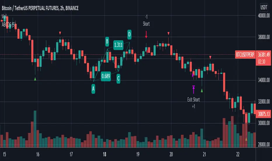
ABCD StrategyOne from many harmonic pattern that consists of two equivalent price legs. The ABCD pattern that helps traders predict when the price is about to change direction.
Tracing And Calculation
This code using pivot high and pivot low built-in method and calculate with Fibonacci Retracement.
Limitation
To find ABCD pattern is very difficult, just coming up a few from thousand candle. That why this code using little bit tolerance ratio to get more pattern.
Cyclic RSI High Low With Noise Filter█ OVERVIEW
This indicator displays Cyclic Relative Strength Index based on Decoding the Hidden Market Rhythm, Part 1 written by Lars von Thienen.
To determine true or false for Overbought / Oversold are unnecessary, therefore these should be either strong or weak.
Noise for weak Overbought / Oversold can be filtered, especially for smaller timeframe.
█ FEATURES
Display calculated Cyclic Relative Strength Index.
Zigzag high low based on Cyclic Relative Strength Index.
Able to filter noise for high low.
█ LEGENDS
◍ Weak Overbought / Oversold
OB ▼ = Strong Overbought
OS ▲ = Strong Oversold
█ USAGE / TIPS
Recommend to be used for Harmonic Patterns such as XABCD and ABCD.
Condition 1 (XABCD) : When ▼ and ▲ exist side by side, usually this outline XA, while the next two ◍ can be BC.
Condition 2 (ABCD) : When ▼ and ▲ exist side by side, usually this outline AB, while the next one ◍ can be BC, strong ABCD.
Condition 3 (ABCD) : When ▼ or ▲ exist at Point A, the next two ◍ can be Point B and Point C, medium ABCD.
Condition 4 (ABCD) : When ◍ exist at Point a, the next two ◍ can be Point b and Point c, weak ABCD usually used as lower case as abcd.
█ CREDITS
LoneSomeTheBlue
WhenToTrade

Pythagorean Means of Moving AveragesDESCRIPTION
Pythagorean Means of Moving Averages
1. Calculates a set of moving averages for high, low, close, open and typical prices, each at multiple periods.
Period values follow the Fibonacci sequence.
The "short" set includes moving average having the following periods: 5, 8, 13, 21, 34, 55, 89, 144, 233, 377.
The "mid" set includes moving average having the following periods: 5, 8, 13, 21, 34, 55, 89, 144, 233, 377, 610, 987, 1597.
The "long" set includes moving average having the following periods: 5, 8, 13, 21, 34, 55, 89, 144, 233, 377, 610, 987, 1597, 2584, 4181.
2. User selects the type of moving average: SMA, EMA, HMA, RMA, WMA, VWMA.
3. Calculates the mean of each set of moving averages.
4. User selects the type of mean to be calculated: 1) arithmetic, 2) geometric, 3) harmonic, 4) quadratic, 5) cubic. Multiple mean calculations may be displayed simultaneously, allowing for comparison.
5. Plots the mean for high, low, close, open, and typical prices.
6. User selects which plots to display: 1) high and low prices, 2) close prices, 3) open prices, and/or 4) typical prices.
7. Calculates and plots a vertical deviation from an origin mean--the mean from which the deviation is measured.
8. Deviation = origin mean x a x b^(x/y)/c.
9. User selects the deviation origin mean: 1) high and low prices plot, 2) close prices plot, or 3) typical prices plot.
10. User defines deviation variables a, b, c, x and y.
Examples of deviation:
a) Percent of the mean = 1.414213562 = 2^(1/2) = Pythagoras's constant (default).
b) Percent of the mean = 0.7071067812 = = = sin 45˚ = cos 45˚.
11. Displaces the plots horizontally +/- by a user defined number of periods.
PURPOSE
1. Identify price trends and potential levels of support and resistance.
CREDITS
1. "Fibonacci Moving Average" by Sofien Kaabar: two plots, each an arithmetic mean of EMAs of 1) high prices and 2) low prices, with periods 5, 8, 13, 21, 34, 55, 89, 144, 233, 377, 610, 987, 1597, 2584, 4181.
2. "Solarized" color scheme by Ethan Schoonover.

Divergence-Support/ResistenceAnother script based on zigzag, divergence, and to yield support and resistence levels.
This idea started with below two concepts:
▶ Support and resistence are simply levels where price has rejected to go further down or up. Usually, we can derive this based on pivots. But, if we start looking at every pivot, there will be many of them and may be confusing to understand which one to consider.
▶ Lot of people asked about one of my previous script on divergence detector on how to use it. I believe divergence should be considered as area of support and resistence because, they only amount to temporary weakness in momentum and nothing more. As per my understanding
Trend > Hidden Divergence > Divergence > Oscillator Levels of Overbought and Oversold
⬜ Process
▶ Now combining the above two concepts - what we are trying to do here is draw support resistence lines only on pivots which has observed either divergence or hidden divergence. Continuation and indecision pivots are ignored.
▶ Input requires only few parameters.
Zigzag lengths and oscillator to be used. Oscillator periods are automatically calculated based on zigzag length. Hence no other information required. You can also chose custom oscillator via external source.
▶ Display include horizontal lines of support/resistence which are drawn from the candle from where divergence or hidden divergence is detected.
▶ Support resistence lines are colored based on divergence. Green shades for bullish divergence and bullish hidden divergence whereas red shades for bearish divervence and bearish hidden divergence. Please note, red and green lines does not mean they only provide resistence or support. Any lines which are below the price should be treated as support and any line which are above the price should be treated as resistence.
▶ Divergence symbols are also printed on the bar from where divergence/hidden divergence is detected.
↗ - Bullish Hidden Divergence
↘ - Bearish Hidden Divergence
⤴ - Bullish Divergence
⤵ - Bearish Divergence
▶ Script also demonstrates usage of libraries effectively. I have used following libraries in this code.
import HeWhoMustNotBeNamed/ zigzag /2 as zg
import HeWhoMustNotBeNamed/enhanced_ta/8 as eta
import HeWhoMustNotBeNamed/ supertrend /4 as st
Can be good combination to use it with harmonic patterns.

Zigzag SARThis is another ZigZag script. But the difference between this and other ZigZag indicators on TV is that here we find highs and lows based on Parabolic SAR.
It repaints?
YES.
On last line of ZigZag you get repainting, because the highs and lows get confirmation only if direction (SAR dots) changes.
This shouldn't be used to forecast highs and lows directly anyway, it's just a visual guide for past highs and lows.
I'm using it to spot harmonic patterns and Wolfe waves more easily. The plan is to draw these automatically in the future, but my skills at Pinescript are limited at the moment.
PS. Ideas for my scripts are coming from @Jegejig1 on Stocktwits, if you want to know who to blame lol

Multi Level ZigzagAt first I thought of doing double zig zag. Once developed I thought it is not much effort to make it multi level zigzag. This script is not same as multi-zigzag indicator (link in the end). In multi zigzag indicator we use zigzag based on different length and each zigzag has no relation to each other. In this script however, each zigzags are related to each other. We cannot just derive Zigzag 4 without deriving Zigzag 3. (Though we can hide each of them individually)
The logic is simple.
Zigzag1: This is the basic zigzag plotted based on given length.
Zigzag2, Zigzag2, Zigzag3 : These are built based on lower level zigzags.
For example, Zigzag2 is built based on Zigzag1 pivots. For calculation, we just use N*2 number of Zigzag1 pivots to derive the next level. Similarly Zigzag2 will become input for Zigzag 3 and Zigzag3 will become input for Zigzag4
Input parameters allow you to chose upto 4 levels of zigzag along with zigzag line color and length. Max array lines also defines how many lines back you want to calculate the zigzag pivots and display then in the stats. Lowering this number will not reduce the number of lines - but, it will limit possibility of calculating higher level zigzags. Stats table just highlight which pivots are applicable for which outer level.
Application: Can be used in pattern recognization scripts to improve accuracy.
Disclaimer: This is not working in intraday charts. Nothing I could do at this point of time. Use it only for daily + timeframes.
Related scripts:
