Breakout Trend Trading Strategy - V1Strategy in nutshell:
This strategy is made to be used in daily time-frames. Works better on trending instruments where volume is available. Hence, this is more suitable for trending shares rather than currencies, commodities and indexes where volume data is either not present or not reliable.
Breakout signifies the continuation of trend. Hence, trade in the direction of breakouts. Breakouts are calculated based on high volume and price movement in a day. This will be combined with few other conditions to generate buy and sell signals along with stop and compound targets. Supertrend is used for trend bias. Our buy and sell targets do not directly depend on the bias. But, entry criteria in opposite trend is made much difficult than that of trend direction. Further explanation of method and input parameters are explained below.
Backtesting parameters :
Capital and position sizing : Capital and position sizing parameters are set to test investing 2000 wholly on certain stock without compounding.
Initial Capital : 2000
Order Size : 100% of equity
Pyramiding : 1
ExitOnSignal : If unchecked exit is triggered solely on trailing stop
Trade Direction : Long, Short or All. Short condition is riskier than long conditions and often results in losses as per my observation. On most of the stocks trending up, strategy will not generate any short signals. This is achieved by comparing yearly high lows to previous two years to decide whether to allow short or long entries.
allowImmediateCompound : Applicable only if compounding/pyramiding is enabled in trade. If checked allows to place compounding orders immediately. If unchecked, it waits for stopline to cross order price before placing next compound.
Display Mode :
Targets : Whenever breakout happens, show marker for upTarget and downTarget
TargetChannel : Show up target and downtarget as a channel
Target With Stop : Along with targets, show also stop levels for breakouts
Up Channel : Channel created from UpTarget and respective stops
Down Channel : Channel created from DownTarget and respective stops
ShowTrailingStop : Shows trailing stop and compound lines when there is a trading position.
ShowTargetLevels : Shows Buy Sell target levels along with stop and compound lines. Trades are done as market orders. Hence, target levels are displayed after strategy makes the trade. Since only one order allowed per side without compounding, target, stop and compound levels are shown sometimes even without trade being made. These can be considered as entry levels if there is no existing position.
ShowPreviousLevels : Shows previous buy/sell target levels. When enabled, layout can look messy.
StopMultiplyer: To Set trailing stop loss.
BacktestYears: Number of years to include in backtest
So far my test cases are:
Positive : AAPL, AMZN, TSLA, RUN, VRT, ASX:APT
Negative Test Cases: WPL, WHC, NHC, WOW, COL, NAB (All ASX stocks)
Special test case: WDI
Negative test cases still show losses in backtesting. I have attempted including many conditions to eliminate or reduce the loss. But, further efforts has resulted in reduction in profits in positive cases as well. Still experimenting. Will update whenever I find improvements. Comments and suggestions welcome :)
Cari dalam skrip untuk "order"

The Maker StrategyDESCRIPTION
The Maker Strategy is a trend-following system built around exponential moving averages (EMAs). By analyzing the alignment of multiple EMAs, the strategy identifies strong bullish or bearish momentum and generates precise entry signals. This method is designed to capture sustained trends while filtering out sideways or noisy market conditions.
USER INPUTS :
• EMA 1 Length (Default: 30)
• EMA 2 Length (Default: 35)
• EMA 3 Length (Default: 40)
• EMA 4 Length (Default: 45)
• EMA 5 Length (Default: 50)
• EMA 6 Length (Default: 60)
LONG CONDITION :
A long signal is triggered when all EMAs are perfectly aligned in ascending order:
EMA1 > EMA2 > EMA3 > EMA4 > EMA5 > EMA6
SHORT CONDITION :
A short signal is triggered when all EMAs are perfectly aligned in descending order:
EMA1 < EMA2 < EMA3 < EMA4 < EMA5 < EMA6
WHY IT IS UNIQUE:
Unlike traditional EMA crossover systems that rely on just 2 or 3 moving averages, The Maker Strategy uses 6 EMAs in sequence. This ensures that trades are only taken when there is clear and strong market momentum. The approach minimizes false signals in ranging markets and focuses on capturing trends with higher probability setups.
HOW USER CAN BENEFIT FROM IT :
• Clear entry alerts for both long and short positions.
• Visual confirmation through candle coloring and EMA band fills.
• Works on multiple timeframes and instruments (stocks, forex, crypto, indices).
• Helps traders stay on the right side of the trend while avoiding whipsaws.
• A simple yet effective tool for those who want a disciplined, rules-based strategy.

Aetherium Institutional Market Resonance EngineAetherium Institutional Market Resonance Engine (AIMRE)
A Three-Pillar Framework for Decoding Institutional Activity
🎓 THEORETICAL FOUNDATION
The Aetherium Institutional Market Resonance Engine (AIMRE) is a multi-faceted analysis system designed to move beyond conventional indicators and decode the market's underlying structure as dictated by institutional capital flow. Its philosophy is built on a singular premise: significant market moves are preceded by a convergence of context , location , and timing . Aetherium quantifies these three dimensions through a revolutionary three-pillar architecture.
This system is not a simple combination of indicators; it is an integrated engine where each pillar's analysis feeds into a central logic core. A signal is only generated when all three pillars achieve a state of resonance, indicating a high-probability alignment between market organization, key liquidity levels, and cyclical momentum.
⚡ THE THREE-PILLAR ARCHITECTURE
1. 🌌 PILLAR I: THE COHERENCE ENGINE (THE 'CONTEXT')
Purpose: To measure the degree of organization within the market. This pillar answers the question: " Is the market acting with a unified purpose, or is it chaotic and random? "
Conceptual Framework: Institutional campaigns (accumulation or distribution) create a non-random, organized market environment. Retail-driven or directionless markets are characterized by "noise" and chaos. The Coherence Engine acts as a filter to ensure we only engage when institutional players are actively steering the market.
Formulaic Concept:
Coherence = f(Dominance, Synchronization)
Dominance Factor: Calculates the absolute difference between smoothed buying pressure (volume-weighted bullish candles) and smoothed selling pressure (volume-weighted bearish candles), normalized by total pressure. A high value signifies a clear winner between buyers and sellers.
Synchronization Factor: Measures the correlation between the streams of buying and selling pressure over the analysis window. A high positive correlation indicates synchronized, directional activity, while a negative correlation suggests choppy, conflicting action.
The final Coherence score (0-100) represents the percentage of market organization. A high score is a prerequisite for any signal, filtering out unpredictable market conditions.
2. 💎 PILLAR II: HARMONIC LIQUIDITY MATRIX (THE 'LOCATION')
Purpose: To identify and map high-impact institutional footprints. This pillar answers the question: " Where have institutions previously committed significant capital? "
Conceptual Framework: Large institutional orders leave indelible marks on the market in the form of anomalous volume spikes at specific price levels. These are not random occurrences but are areas of intense historical interest. The Harmonic Liquidity Matrix finds these footprints and consolidates them into actionable support and resistance zones called "Harmonic Nodes."
Algorithmic Process:
Footprint Identification: The engine scans the historical lookback period for candles where volume > average_volume * Institutional_Volume_Filter. This identifies statistically significant volume events.
Node Creation: A raw node is created at the mean price of the identified candle.
Dynamic Clustering: The engine uses an ATR-based proximity algorithm. If a new footprint is identified within Node_Clustering_Distance (ATR) of an existing Harmonic Node, it is merged. The node's price is volume-weighted, and its magnitude is increased. This prevents chart clutter and consolidates nearby institutional orders into a single, more significant level.
Node Decay: Nodes that are older than the Institutional_Liquidity_Scanback period are automatically removed from the chart, ensuring the analysis remains relevant to recent market dynamics.
3. 🌊 PILLAR III: CYCLICAL RESONANCE MATRIX (THE 'TIMING')
Purpose: To identify the market's dominant rhythm and its current phase. This pillar answers the question: " Is the market's immediate energy flowing up or down? "
Conceptual Framework: Markets move in waves and cycles of varying lengths. Trading in harmony with the current cyclical phase dramatically increases the probability of success. Aetherium employs a simplified wavelet analysis concept to decompose price action into short, medium, and long-term cycles.
Algorithmic Process:
Cycle Decomposition: The engine calculates three oscillators based on the difference between pairs of Exponential Moving Averages (e.g., EMA8-EMA13 for short cycle, EMA21-EMA34 for medium cycle).
Energy Measurement: The 'energy' of each cycle is determined by its recent volatility (standard deviation). The cycle with the highest energy is designated as the "Dominant Cycle."
Phase Analysis: The engine determines if the dominant cycles are in a bullish phase (rising from a trough) or a bearish phase (falling from a peak).
Cycle Sync: The highest conviction timing signals occur when multiple cycles (e.g., short and medium) are synchronized in the same direction, indicating broad-based momentum.
🔧 COMPREHENSIVE INPUT SYSTEM
Pillar I: Market Coherence Engine
Coherence Analysis Window (10-50, Default: 21): The lookback period for the Coherence Engine.
Lower Values (10-15): Highly responsive to rapid shifts in market control. Ideal for scalping but can be sensitive to noise.
Balanced (20-30): Excellent for day trading, capturing the ebb and flow of institutional sessions.
Higher Values (35-50): Smoother, more stable reading. Best for swing trading and identifying long-term institutional campaigns.
Coherence Activation Level (50-90%, Default: 70%): The minimum market organization required to enable signal generation.
Strict (80-90%): Only allows signals in extremely clear, powerful trends. Fewer, but potentially higher quality signals.
Standard (65-75%): A robust filter that effectively removes choppy conditions while capturing most valid institutional moves.
Lenient (50-60%): Allows signals in less-organized markets. Can be useful in ranging markets but may increase false signals.
Pillar II: Harmonic Liquidity Matrix
Institutional Liquidity Scanback (100-400, Default: 200): How far back the engine looks for institutional footprints.
Short (100-150): Focuses on recent institutional activity, providing highly relevant, immediate levels.
Long (300-400): Identifies major, long-term structural levels. These nodes are often extremely powerful but may be less frequent.
Institutional Volume Filter (1.3-3.0, Default: 1.8): The multiplier for detecting a volume spike.
High (2.5-3.0): Only registers climactic, undeniable institutional volume. Fewer, but more significant nodes.
Low (1.3-1.7): More sensitive, identifying smaller but still relevant institutional interest.
Node Clustering Distance (0.2-0.8 ATR, Default: 0.4): The ATR-based distance for merging nearby nodes.
High (0.6-0.8): Creates wider, more consolidated zones of liquidity.
Low (0.2-0.3): Creates more numerous, precise, and distinct levels.
Pillar III: Cyclical Resonance Matrix
Cycle Resonance Analysis (30-100, Default: 50): The lookback for determining cycle energy and dominance.
Short (30-40): Tunes the engine to faster, shorter-term market rhythms. Best for scalping.
Long (70-100): Aligns the timing component with the larger primary trend. Best for swing trading.
Institutional Signal Architecture
Signal Quality Mode (Professional, Elite, Supreme): Controls the strictness of the three-pillar confluence.
Professional: Loosest setting. May generate signals if two of the three pillars are in strong alignment. Increases signal frequency.
Elite: Balanced setting. Requires a clear, unambiguous resonance of all three pillars. The recommended default.
Supreme: Most stringent. Requires perfect alignment of all three pillars, with each pillar exhibiting exceptionally strong readings (e.g., coherence > 85%). The highest conviction signals.
Signal Spacing Control (5-25, Default: 10): The minimum bars between signals to prevent clutter and redundant alerts.
🎨 ADVANCED VISUAL SYSTEM
The visual architecture of Aetherium is designed not merely for aesthetics, but to provide an intuitive, at-a-glance understanding of the complex data being processed.
Harmonic Liquidity Nodes: The core visual element. Displayed as multi-layered, semi-transparent horizontal boxes.
Magnitude Visualization: The height and opacity of a node's "glow" are proportional to its volume magnitude. More significant nodes appear brighter and larger, instantly drawing the eye to key levels.
Color Coding: Standard nodes are blue/purple, while exceptionally high-magnitude nodes are highlighted in an accent color to denote critical importance.
🌌 Quantum Resonance Field: A dynamic background gradient that visualizes the overall market environment.
Color: Shifts from cool blues/purples (low coherence) to energetic greens/cyans (high coherence and organization), providing instant context.
Intensity: The brightness and opacity of the field are influenced by total market energy (a composite of coherence, momentum, and volume), making powerful market states visually apparent.
💎 Crystalline Lattice Matrix: A geometric web of lines projected from a central moving average.
Mathematical Basis: Levels are projected using multiples of the Golden Ratio (Phi ≈ 1.618) and the ATR. This visualizes the natural harmonic and fractal structure of the market. It is not arbitrary but is based on mathematical principles of market geometry.
🧠 Synaptic Flow Network: A dynamic particle system visualizing the engine's "thought process."
Node Density & Activation: The number of particles and their brightness/color are tied directly to the Market Coherence score. In high-coherence states, the network becomes a dense, bright, and organized web. In chaotic states, it becomes sparse and dim.
⚡ Institutional Energy Waves: Flowing sine waves that visualize market volatility and rhythm.
Amplitude & Speed: The height and speed of the waves are directly influenced by the ATR and volume, providing a feel for market energy.
📊 INSTITUTIONAL CONTROL MATRIX (DASHBOARD)
The dashboard is the central command console, providing a real-time, quantitative summary of each pillar's status.
Header: Displays the script title and version.
Coherence Engine Section:
State: Displays a qualitative assessment of market organization: ◉ PHASE LOCK (High Coherence), ◎ ORGANIZING (Moderate Coherence), or ○ CHAOTIC (Low Coherence). Color-coded for immediate recognition.
Power: Shows the precise Coherence percentage and a directional arrow (↗ or ↘) indicating if organization is increasing or decreasing.
Liquidity Matrix Section:
Nodes: Displays the total number of active Harmonic Liquidity Nodes currently being tracked.
Target: Shows the price level of the nearest significant Harmonic Node to the current price, representing the most immediate institutional level of interest.
Cycle Matrix Section:
Cycle: Identifies the currently dominant market cycle (e.g., "MID ") based on cycle energy.
Sync: Indicates the alignment of the cyclical forces: ▲ BULLISH , ▼ BEARISH , or ◆ DIVERGENT . This is the core timing confirmation.
Signal Status Section:
A unified status bar that provides the final verdict of the engine. It will display "QUANTUM SCAN" during neutral periods, or announce the tier and direction of an active signal (e.g., "◉ TIER 1 BUY ◉" ), highlighted with the appropriate color.
🎯 SIGNAL GENERATION LOGIC
Aetherium's signal logic is built on the principle of strict, non-negotiable confluence.
Condition 1: Context (Coherence Filter): The Market Coherence must be above the Coherence Activation Level. No signals can be generated in a chaotic market.
Condition 2: Location (Liquidity Node Interaction): Price must be actively interacting with a significant Harmonic Liquidity Node.
For a Buy Signal: Price must be rejecting the Node from below (testing it as support).
For a Sell Signal: Price must be rejecting the Node from above (testing it as resistance).
Condition 3: Timing (Cycle Alignment): The Cyclical Resonance Matrix must confirm that the dominant cycles are synchronized with the intended trade direction.
Signal Tiering: The Signal Quality Mode input determines how strictly these three conditions must be met. 'Supreme' mode, for example, might require not only that the conditions are met, but that the Market Coherence is exceptionally high and the interaction with the Node is accompanied by a significant volume spike.
Signal Spacing: A final filter ensures that signals are spaced by a minimum number of bars, preventing over-alerting in a single move.
🚀 ADVANCED TRADING STRATEGIES
The Primary Confluence Strategy: The intended use of the system. Wait for a Tier 1 (Elite/Supreme) or Tier 2 (Professional/Elite) signal to appear on the chart. This represents the alignment of all three pillars. Enter after the signal bar closes, with a stop-loss placed logically on the other side of the Harmonic Node that triggered the signal.
The Coherence Context Strategy: Use the Coherence Engine as a standalone market filter. When Coherence is high (>70%), favor trend-following strategies. When Coherence is low (<50%), avoid new directional trades or favor range-bound strategies. A sharp drop in Coherence during a trend can be an early warning of a trend's exhaustion.
Node-to-Node Trading: In a high-coherence environment, use the Harmonic Liquidity Nodes as both entry points and profit targets. For example, after a BUY signal is generated at one Node, the next Node above it becomes a logical first profit target.
⚖️ RESPONSIBLE USAGE AND LIMITATIONS
Decision Support, Not a Crystal Ball: Aetherium is an advanced decision-support tool. It is designed to identify high-probability conditions based on a model of institutional behavior. It does not predict the future.
Risk Management is Paramount: No indicator can replace a sound risk management plan. Always use appropriate position sizing and stop-losses. The signals provided are probabilistic, not certainties.
Past Performance Disclaimer: The market models used in this script are based on historical data. While robust, there is no guarantee that these patterns will persist in the future. Market conditions can and do change.
Not a "Set and Forget" System: The indicator performs best when its user understands the concepts behind the three pillars. Use the dashboard and visual cues to build a comprehensive view of the market before acting on a signal.
Backtesting is Essential: Before applying this tool to live trading, it is crucial to backtest and forward-test it on your preferred instruments and timeframes to understand its unique behavior and characteristics.
🔮 CONCLUSION
The Aetherium Institutional Market Resonance Engine represents a paradigm shift from single-variable analysis to a holistic, multi-pillar framework. By quantifying the abstract concepts of market context, location, and timing into a unified, logical system, it provides traders with an unprecedented lens into the mechanics of institutional market operations.
It is not merely an indicator, but a complete analytical engine designed to foster a deeper understanding of market dynamics. By focusing on the core principles of institutional order flow, Aetherium empowers traders to filter out market noise, identify key structural levels, and time their entries in harmony with the market's underlying rhythm.
"In all chaos there is a cosmos, in all disorder a secret order." - Carl Jung
— Dskyz, Trade with insight. Trade with confluence. Trade with Aetherium.

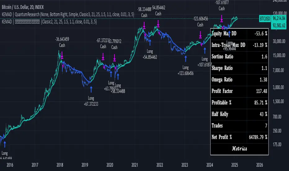
KEMAD | QuantumResearchQuantumResearch KEMAD Indicator
The QuantumResearch KEMAD Indicator is a sophisticated trend-following and volatility-based tool designed for traders who demand precision in detecting market trends and price reversals. By leveraging advanced techniques implemented in PineScript, this indicator integrates a Kalman filter, an Exponential Moving Average (EMA), and dynamic ATR-based deviation bands to produce clear, actionable trading signals.
1. Overview
The KEMAD Indicator aims to:
Reduce Market Noise: Employ a Kalman filter to smooth price data.
Identify Trends: Use an EMA of the filtered price to define the prevailing market direction.
Set Dynamic Thresholds: Adjust breakout levels with ATR-based deviation bands.
Generate Signals: Provide clear long and short trading signals along with intuitive visual cues.
2. How It Works
A. Kalman Filter Smoothing
Purpose: The Kalman filter refines the selected price source (e.g., close price) by reducing short-term fluctuations, thus offering a clearer view of the underlying price movement.
Customization: Users can adjust key parameters such as:
Process Noise: Controls the filter’s sensitivity to recent changes.
Measurement Noise: Determines how responsive the filter is to incoming price data.
Filter Order: Sets the number of data points considered in the smoothing process.
B. EMA-Based Trend Detection
Primary Trend EMA: A 25-period EMA is applied to the Kalman-filtered price, serving as the core trend indicator.
Signal Mechanism:
Long Signal: Triggered when the price exceeds the EMA plus an ATR-based upper deviation.
Short Signal: Triggered when the price falls below the EMA minus an ATR-based lower deviation.
C. ATR Deviation Bands
ATR Utilization: The Average True Range (ATR) is computed (default length of 21) to assess market volatility.
Dynamic Thresholds:
Upper Deviation: Calculated by adding 1.5× ATR to the EMA (for long signals).
Lower Deviation: Calculated by subtracting 1.1× ATR from the EMA (for short signals).
These bands adapt to current volatility, ensuring that signal thresholds are both dynamic and market-sensitive.
3. Visual Representation
The indicator’s design emphasizes clarity and ease of use:
Color-Coded Bar Signals:
Green Bars: Indicate bullish conditions when a long signal is active.
Red Bars: Indicate bearish conditions when a short signal is active.
Trend Confirmation Line: A 54-period EMA is plotted to further validate trend direction. Its color dynamically changes to reflect the active trend.
Background Fill: The space between a calculated price midpoint (typically the average of high and low) and the EMA is filled, visually emphasizing the prevailing market trend.
4. Customization & Parameters
The KEMAD Indicator is highly configurable, allowing traders to tailor the tool to their specific trading strategies and market conditions:
ATR Settings:
ATR Length: Default is 21; adjusts sensitivity to market volatility.
EMA Settings:
Trend EMA Length: Default is 25; smooths price action for trend detection.
Confirmation EMA Length: Default is 54; aids in confirming the trend.
Kalman Filter Parameters:
Process Noise: Default is 0.01.
Measurement Noise: Default is 3.0.
Filter Order: Default is 5.
Deviation Multipliers:
Long Signal Multiplier: Default is 1.5× ATR.
Short Signal Multiplier: Default is 1.1× ATR.
Appearance: Eight customizable color themes are available to suit individual visual preferences.
5. Trading Applications
The versatility of the KEMAD Indicator makes it suitable for various trading strategies:
Trend Following: It helps identify and ride sustained bullish or bearish trends by filtering out market noise.
Breakout Trading: Detects when prices move beyond the ATR-based deviation bands, signaling potential breakout opportunities.
Reversal Detection: Alerts traders to potential trend reversals when price crosses the dynamically smoothed EMA.
Risk Management: Offers clearly defined entry and exit points, based on volatility-adjusted thresholds, enhancing trade precision and risk control.
6. Final Thoughts
The QuantumResearch KEMAD Indicator represents a unique blend of advanced filtering (via the Kalman filter), robust trend analysis (using EMAs), and dynamic volatility assessment (through ATR deviation bands).
Its PineScript implementation allows for a high degree of customization, making it an invaluable tool for traders looking to reduce noise, accurately detect trends, and manage risk effectively.
Whether used for trend following, breakout strategies, or reversal detection, the KEMAD Indicator is designed to adapt to varying market conditions and trading styles.
Important Disclaimer: Past data does not predict future behavior. This indicator is provided for informational purposes only; no indicator or strategy can guarantee future results. Always perform thorough analysis and use proper risk management before trading.
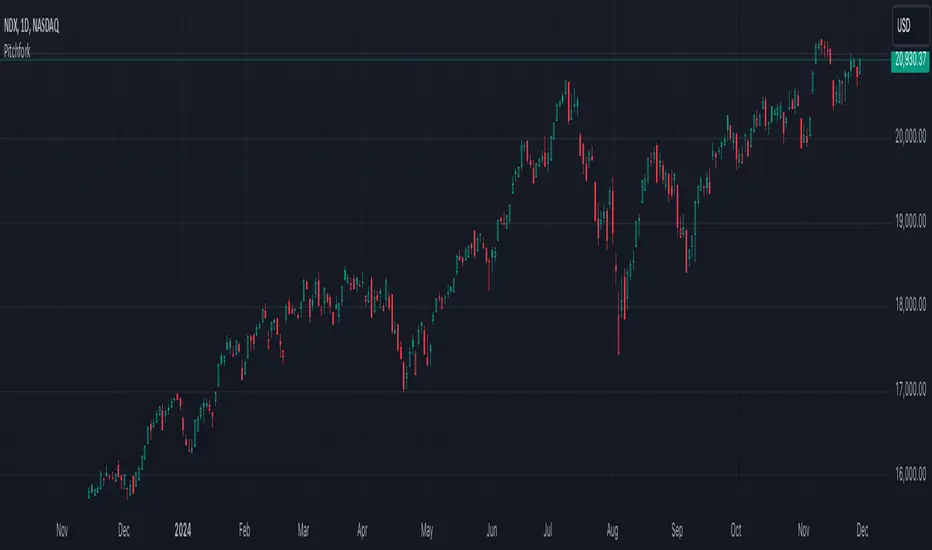
PitchforkLibrary "Pitchfork"
Pitchfork class
method tostring(this)
Converts PitchforkTypes/Fork object to string representation
Namespace types: Fork
Parameters:
this (Fork) : PitchforkTypes/Fork object
Returns: string representation of PitchforkTypes/Fork
method tostring(this)
Converts Array of PitchforkTypes/Fork object to string representation
Namespace types: array
Parameters:
this (array) : Array of PitchforkTypes/Fork object
Returns: string representation of PitchforkTypes/Fork array
method tostring(this, sortKeys, sortOrder)
Converts PitchforkTypes/PitchforkProperties object to string representation
Namespace types: PitchforkProperties
Parameters:
this (PitchforkProperties) : PitchforkTypes/PitchforkProperties object
sortKeys (bool) : If set to true, string output is sorted by keys.
sortOrder (int) : Applicable only if sortKeys is set to true. Positive number will sort them in ascending order whreas negative numer will sort them in descending order. Passing 0 will not sort the keys
Returns: string representation of PitchforkTypes/PitchforkProperties
method tostring(this, sortKeys, sortOrder)
Converts PitchforkTypes/PitchforkDrawingProperties object to string representation
Namespace types: PitchforkDrawingProperties
Parameters:
this (PitchforkDrawingProperties) : PitchforkTypes/PitchforkDrawingProperties object
sortKeys (bool) : If set to true, string output is sorted by keys.
sortOrder (int) : Applicable only if sortKeys is set to true. Positive number will sort them in ascending order whreas negative numer will sort them in descending order. Passing 0 will not sort the keys
Returns: string representation of PitchforkTypes/PitchforkDrawingProperties
method tostring(this, sortKeys, sortOrder)
Converts PitchforkTypes/Pitchfork object to string representation
Namespace types: Pitchfork
Parameters:
this (Pitchfork) : PitchforkTypes/Pitchfork object
sortKeys (bool) : If set to true, string output is sorted by keys.
sortOrder (int) : Applicable only if sortKeys is set to true. Positive number will sort them in ascending order whreas negative numer will sort them in descending order. Passing 0 will not sort the keys
Returns: string representation of PitchforkTypes/Pitchfork
method createDrawing(this)
Creates PitchforkTypes/PitchforkDrawing from PitchforkTypes/Pitchfork object
Namespace types: Pitchfork
Parameters:
this (Pitchfork) : PitchforkTypes/Pitchfork object
Returns: PitchforkTypes/PitchforkDrawing object created
method createDrawing(this)
Creates PitchforkTypes/PitchforkDrawing array from PitchforkTypes/Pitchfork array of objects
Namespace types: array
Parameters:
this (array) : array of PitchforkTypes/Pitchfork object
Returns: array of PitchforkTypes/PitchforkDrawing object created
method draw(this)
draws from PitchforkTypes/PitchforkDrawing object
Namespace types: PitchforkDrawing
Parameters:
this (PitchforkDrawing) : PitchforkTypes/PitchforkDrawing object
Returns: PitchforkTypes/PitchforkDrawing object drawn
method delete(this)
deletes PitchforkTypes/PitchforkDrawing object
Namespace types: PitchforkDrawing
Parameters:
this (PitchforkDrawing) : PitchforkTypes/PitchforkDrawing object
Returns: PitchforkTypes/PitchforkDrawing object deleted
method delete(this)
deletes underlying drawing of PitchforkTypes/Pitchfork object
Namespace types: Pitchfork
Parameters:
this (Pitchfork) : PitchforkTypes/Pitchfork object
Returns: PitchforkTypes/Pitchfork object deleted
method delete(this)
deletes array of PitchforkTypes/PitchforkDrawing objects
Namespace types: array
Parameters:
this (array) : Array of PitchforkTypes/PitchforkDrawing object
Returns: Array of PitchforkTypes/PitchforkDrawing object deleted
method delete(this)
deletes underlying drawing in array of PitchforkTypes/Pitchfork objects
Namespace types: array
Parameters:
this (array) : Array of PitchforkTypes/Pitchfork object
Returns: Array of PitchforkTypes/Pitchfork object deleted
method clear(this)
deletes array of PitchforkTypes/PitchforkDrawing objects and clears the array
Namespace types: array
Parameters:
this (array) : Array of PitchforkTypes/PitchforkDrawing object
Returns: void
method clear(this)
deletes array of PitchforkTypes/Pitchfork objects and clears the array
Namespace types: array
Parameters:
this (array) : Array of Pitchfork/Pitchfork object
Returns: void
PitchforkDrawingProperties
Pitchfork Drawing Properties object
Fields:
extend (series bool) : If set to true, forks are extended towards right. Default is true
fill (series bool) : Fill forklines with transparent color. Default is true
fillTransparency (series int) : Transparency at which fills are made. Only considered when fill is set. Default is 80
forceCommonColor (series bool) : Force use of common color for forks and fills. Default is false
commonColor (series color) : common fill color. Used only if ratio specific fill colors are not available or if forceCommonColor is set to true.
PitchforkDrawing
Pitchfork drawing components
Fields:
medianLine (Line type from Trendoscope/Drawing/2) : Median line of the pitchfork
baseLine (Line type from Trendoscope/Drawing/2) : Base line of the pitchfork
forkLines (array type from Trendoscope/Drawing/2) : fork lines of the pitchfork
linefills (array type from Trendoscope/Drawing/2) : Linefills between forks
Fork
Fork object property
Fields:
ratio (series float) : Fork ratio
forkColor (series color) : color of fork. Default is blue
include (series bool) : flag to include the fork in drawing. Default is true
PitchforkProperties
Pitchfork Properties
Fields:
forks (array) : Array of Fork objects
type (series string) : Pitchfork type. Supported values are "regular", "schiff", "mschiff", Default is regular
inside (series bool) : Flag to identify if to draw inside fork. If set to true, inside fork will be drawn
Pitchfork
Pitchfork object
Fields:
a (chart.point) : Pivot Point A of pitchfork
b (chart.point) : Pivot Point B of pitchfork
c (chart.point) : Pivot Point C of pitchfork
properties (PitchforkProperties) : PitchforkProperties object which determines type and composition of pitchfork
dProperties (PitchforkDrawingProperties) : Drawing properties for pitchfork
lProperties (LineProperties type from Trendoscope/Drawing/2) : Common line properties for Pitchfork lines
drawing (PitchforkDrawing) : PitchforkDrawing object
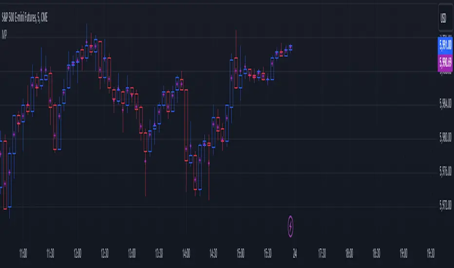
Mean Price
^^ Plotting switched to Line.
This method of financial time series (aka bars) downsampling is literally, naturally, and thankfully the best you can do in terms of maximizing info gain. You can finally chill and feed it to your studies & eyes, and probably use nothing else anymore.
(HL2 and occ3 also have use cases, but other aggregation methods? Not really, even if they do, the use cases are ‘very’ specific). Tho in order to understand why, you gotta read the following wall, or just believe me telling you, ‘I put it on my momma’.
The true story about trading volumes and why this is all a big misdirection
Actually, you don’t need to be a quant to get there. All you gotta do is stop blindly following other people’s contextual (at best) solutions, eg OC2 aggregation xD, and start using your own brain to figure things out.
Every individual trade (basically an imprint on 1D price space that emerges when market orders hit the order book) has several features like: price, time, volume, AND direction (Up if a market buy order hits the asks, Down if a market sell order hits the bids). Now, the last two features—volume and direction—can be effectively combined into one (by multiplying volume by 1 or -1), and this is probably how every order matching engine should output data. If we’re not considering size/direction, we’re leaving data behind. Moreover, trades aren’t just one-price dots all the time. One trade can consume liquidity on several levels of the order book, so a single trade can be several ticks big on the price axis.
You may think now that there are no zero-volume ticks. Well, yes and no. It depends on how you design an exchange and whether you allow intra-spread trades/mid-spread trades (now try to Google it). Intra-spread trades could happen if implemented when a matching engine receives both buy and sell orders at the same microsecond period. This way, you can match the orders with each other at a better price for both parties without even hitting the book and consuming liquidity. Also, if orders have different sizes, the remaining part of the bigger order can be sent to the order book. Basically, this type of trade can be treated as an OTC trade, having zero volume because we never actually hit the book—there’s no imprint. Another reason why it makes sense is when we think about volume as an impact or imbalance act, and how the medium (order book in our case) responds to it, providing information. OTC and mid-spread trades are not aggressive sells or buys; they’re neutral ticks, so to say. However huge they are, sometimes many blocks on NYSE, they don’t move the price because there’s no impact on the medium (again, which is the order book)—they’re not providing information.
... Now, we need to aggregate these trades into, let’s say, 1-hour bars (remember that a trade can have either positive or negative volume). We either don’t want to do it, or we don’t have this kind of information. What we can do is take already aggregated OHLC bars and extract all the info from them. Given the market is fractal, bars & trades gotta have the same set of features:
- Highest & lowest ticks (high & low) <- by price;
- First & last ticks (open & close) <- by time;
- Biggest and smallest ticks <- by volume.*
*e.g., in the array ,
2323: biggest trade,
-1212: smallest trade.
Now, in our world, somehow nobody started to care about the biggest and smallest trades and their inclusion in OHLC data, while this is actually natural. It’s the same way as it’s done with high & low and open & close: we choose the minimum and maximum value of a given feature/axis within the aggregation period.
So, we don’t have these 2 values: biggest and smallest ticks. The best we can do is infer them, and given the fact the biggest and smallest ticks can be located with the same probability everywhere, all we can do is predict them in the middle of the bar, both in time and price axes. That’s why you can see two HL2’s in each of the 3 formulas in the code.
So, summed up absolute volumes that you see in almost every trading platform are actually just a derivative metric, something that I call Type 2 time series in my own (proprietary ‘for now’) methods. It doesn’t have much to do with market orders hitting the non-uniform medium (aka order book); it’s more like a statistic. Still wanna use VWAP? Ok, but you gotta understand you’re weighting Type 1 (natural) time series by Type 2 (synthetic) ones.
How to combine all the data in the right way (khmm khhm ‘order’)
Now, since we have 6 values for each bar, let’s see what information we have about them, what we don’t have, and what we can do about it:
- Open and close: we got both when and where (time (order) and price);
- High and low: we got where, but we don’t know when;
- Biggest & smallest trades: we know shit, we infer it the way it was described before.'
By using the location of the close & open prices relative to the high & low prices, we can make educated guesses about whether high or low was made first in a given bar. It’s not perfect, but it’s ultimately all we can do—this is the very last bit of info we can extract from the data we have.
There are 2 methods for inferring volume delta (which I call simply volume) that are presented everywhere, even here on TradingView. Funny thing is, this is actually 2 parts of the 1 method. I wonder how many folks see through it xD. The same method can be used for both inferring volume delta AND making educated guesses whether high or low was made first.
Imagine and/or find the cases on your charts to understand faster:
* Close > open means we have an up bar and probably the volume is positive, and probably high was made later than low.
* Close < open means we have a down bar and probably the volume is negative, and probably low was made later than high.
Now that’s the point when you see that these 2 mentioned methods are actually parts of the 1 method:
If close = open, we still have another clue: distance from open/close pair to high (HC), and distance from open/close pair to low (LC):
* HC < LC, probably high was made later.
* HC > LC, probably low was made later.
And only if close = open and HC = LC, only in this case we have no clue whether high or low was made earlier within a bar. We simply don’t have any more information to even guess. This bar is called a neutral bar.
At this point, we have both time (order) and price info for each of our 6 values. Now, we have to solve another weighted average problem, and that’s it. We’ll weight prices according to the order we’ve guessed. In the neutral bar case, open has a weight of 1, close has a weight of 3, and both high and low have weights of 2 since we can’t infer which one was made first. In all cases, biggest and smallest ticks are modeled with HL2 and weighted like they’re located in the middle of the bar in a time sense.
P.S.: I’ve also included a "robust" method where all the bars are treated like neutral ones. I’ve used it before; obviously, it has lesser info gain -> works a bit worse.
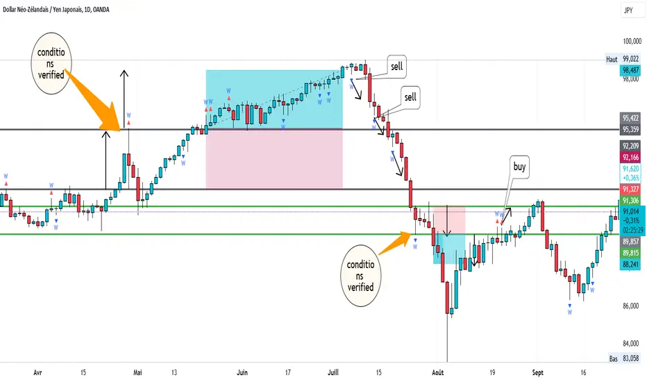
Strategy: Candlestick Wick Analysis with Volume Conditions
This strategy focuses on analyzing the wicks (or shadows) of candlesticks to identify potential trading opportunities based on candlestick structure and volume. Based on these criteria, it places stop orders at the extremities of the wicks when certain conditions are met, thus increasing the chances of capturing significant price movements.
Trading Criteria
Volume Conditions:
The strategy checks if the volume of the current candle is higher than that of the previous three candles. This ensures that the observed price movement is supported by significant volume, increasing the probability that the price will continue in the same direction.
Wick Analysis:
Upper Wick:
If the upper wick of a candle represents more than 90% of its body size and is longer than the lower wick, this indicates that the price tested a resistance level before pulling back.
Order Placement: In this case, a Buy Stop order is placed at the upper extremity of the wick. This means that if the price rises back to this level, the order will be triggered, and the trader will take a buy position.
SL Management: A stop-loss is then placed below the lowest point of the same candle. This protects the trader by limiting losses if the price falls back after the order is triggered.
Lower Wick:
If the lower wick of a candle is longer than the upper wick and represents more than 90% of its body size, this indicates that the price tested a support level before rising.
Order Placement: In this case, a Sell Stop order is placed at the lower extremity of the wick. Thus, if the price drops back to this level, the order will be triggered, and the trader will take a sell position.
SL Management: A stop-loss is then placed above the highest point of the same candle. This ensures risk management by limiting losses if the price rebounds upward after the order is triggered.
Strategy Advantages
Responsiveness to Price Movements: The strategy is designed to detect significant price movements based on the market's reaction around support and resistance levels. By placing stop orders directly at the wick extremities, it allows capturing strong movements in the direction indicated by the candles.
Securing Positions: Using stop-losses positioned just above or below key levels (wicks) provides better risk management. If the market doesn't move as expected, the position is automatically closed with a limited loss.
Clear Visual Indicators: Symbols are displayed on the chart at the points where orders have been placed, making it easier to understand trading decisions. This helps to quickly identify the support or resistance levels tested by the price, as well as potential entry points.
Conclusion
The strategy is based on the idea that large wicks signal areas where buyers or sellers have tested significant price levels before temporarily retreating. By placing stop orders at the extremities of these wicks, the strategy allows capturing price movements when they confirm, while limiting risks through strategically placed stop-losses. It thus offers a balanced approach between capturing potential profit and managing risk.
This description emphasizes the idea of capturing significant market movements with stop orders while providing a clear explanation of the logic and risk management. It’s tailored for publication on TradingView and highlights the robustness of the strategy.
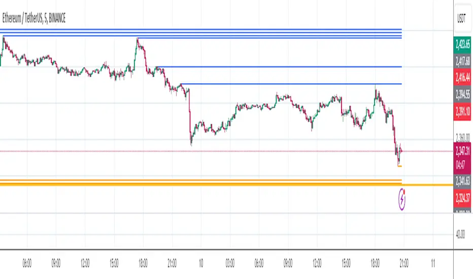
Liquidity VisualizerThe "Liquidity Visualizer" indicator is designed to help traders visualize potential areas of liquidity on a price chart. In trading, liquidity often accumulates around key levels where market participants have placed their stop orders or pending orders. These levels are commonly found at significant highs and lows, where traders tend to set their stop-losses or take-profit orders. The indicator aims to highlight these areas by drawing unbroken lines that extend indefinitely until breached by the price action.
Specifically, this indicator identifies and marks pivot highs and pivot lows, which are price levels where a trend changes direction. When a pivot high or pivot low is formed, it is represented on the chart with a horizontal line that continues to extend until the price touches or surpasses that level. The line remains in place as long as the level remains unbroken, which means there is potential liquidity still resting at that level.
The concept behind this indicator is that liquidity is likely to be resting at unbroken pivot points. These levels are areas where stop-loss orders or pending buy/sell orders may have accumulated, making them attractive zones for large market participants, such as institutions, to target. By visualizing these unbroken levels, traders can gain insight into where liquidity might be concentrated and where potential price reversals or significant movements could occur as liquidity is taken out.
The indicator helps traders make more informed decisions by showing them key price levels that may attract significant market activity. For instance, if a trader sees multiple unbroken pivot high lines above the current price, they might infer that there is a cluster of liquidity in that area, which could lead to a price spike as those levels are breached. Similarly, unbroken pivot lows may indicate areas where downside liquidity is concentrated.
In summary, this indicator acts as a "liquidity visualizer," providing traders with a clear, visual representation of potential liquidity resting at significant pivot points. This information can be valuable for understanding where price might be drawn to, and where large movements might occur as liquidity is targeted and removed by market participants.
Grid TraderGrid Trader Indicator ( GTx ):
Overview
The Grid Trader Indicator is a tool that helps traders visualize key levels within a specified trading range. The indicator plots accumulation and distribution levels, an entry level, an exit level, and a midpoint. This guide will help you understand how to use the indicator and its features for effective grid trading.
Basics of Trading Range, Grid Buy, and Grid Sell
Trading Range
A trading range is the horizontal price movement between a defined upper ( resistance ) and lower ( support ) level over a period of time. When a security trades within a range, it repeatedly moves between these two levels without trending upwards or downwards significantly. Traders often use the trading range to identify potential buy and sell points:
Upper Level (Resistance): This is the price level at which selling pressure overcomes buying pressure, preventing the price from rising further.
Lower Level (Support): This is the price level at which buying pressure overcomes selling pressure, preventing the price from falling further.
Grid Trading Strategy
Grid trading is a type of trading strategy that involves placing buy and sell orders at predefined intervals around a set price. It aims to profit from the natural market volatility by buying low and selling high in a range-bound market. The strategy divides the trading range into several grid levels where orders are placed.
Grid Buy
Grid buy orders are placed at intervals below the current price . When the price drops to these levels, buy orders are triggered . This strategy ensures that the trader buys more as the price falls, potentially lowering the average purchase price .
Grid Sell
Grid sell orders are placed at intervals above the current price . When the price rises to these levels, sell orders are triggered . This ensures that the trader sells portions of their holdings as the price increases, potentially securing profits at higher levels .
Key Points of Grid Trading
Grid Size : The interval between each buy and sell order. This can be constant (e.g., $2 intervals) or variable based on certain conditions.
Accumulation Range : The lower part of the trading range where buy orders are placed.
Distribution Range : The upper part of the trading range where sell orders are placed.
Midpoint : The average price of the entry and exit levels, often used as a reference point for balance.
As the price moves up and down within this range, your buy orders will be triggered as the price drops and your sell orders will be triggered as the price rises. This allows you to accumulate more of the asset at lower prices and sell portions at higher prices, profiting from the price oscillations within the defined range. Grid trading can be particularly effective in a sideways market where there is no clear long-term trend. However, it requires careful monitoring and adjustment of grid levels based on market conditions to minimize risks and maximize returns .
Configuring the Indicator :
Once the indicator is added, you will see a settings icon next to it. Click on it to open the settings menu.
Adjust the Upper Level , Lower Level , Entry Level , and Exit Level to match your trading strategy and market conditions.
Set the Levels Visibility to control how many bars back the levels will be plotted.
Interpreting the Levels :
Accumulation Levels : These are plotted below the entry level and are potential buy zones. They are labeled as Accumulation Level 1, 2, and 3.
Distribution Levels : These are plotted above the exit level and are potential sell zones. They are labeled as Distribution Level 1, 2, and 3.
Upper Level : Marked in fuchsia, indicating the top boundary of the trading range.
Exit Level : Marked in yellow, indicating the level at which you plan to exit trades.
Midpoint : Marked in white, indicating the average of the entry and exit levels.
Entry Level : Marked in yellow, indicating the level at which you plan to enter trades.
Lower Level : Marked in aqua, indicating the bottom boundary of the trading range.
By visualizing key levels, you can make informed decisions on where to place buy and sell orders, potentially maximizing your trading profits through systematic grid trading.

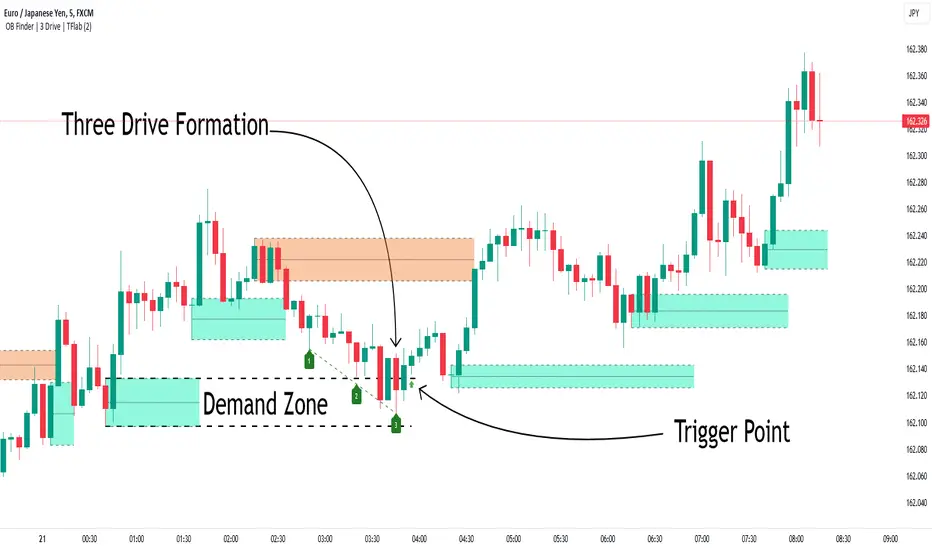
Smart Money Setup 04 [TradingFinder] Three Drive (Harmonic) + OB🔵 Introduction
The "Three Drive" pattern is a well-known formation in technical analysis, recognized for its ability to signal potential trend reversals in price action. Within the realm of trading, particularly in the context of "Reversal Patterns," the Three Drive pattern holds significance as a reliable indicator of shifts in market sentiment.
🟣 Bullish 3 Drive
This pattern typically manifests at a price bottom, where a sequence of lower lows suggests a prevailing negative trend. However, within the structure of the Three Drive pattern, a notable occurrence unfolds.
The second low breaches the range of the first low, followed by the third low surpassing the range of the second low. These penetrations signify a diminishing selling pressure and an emerging buying interest.
Traders often await the confirmation of the third low surpassing the second low as an entry point, with price targets set at the highs formed within the Three Drive pattern.
🟣 Bearish 3 Drive
Conversely, the Bearish Three Drive pattern emerges at a price top, characterized by a sequence of higher highs indicating an upward trend. Yet, amidst this apparent bullish momentum, a shift occurs.
The second high breaks beyond the range of the first high, succeeded by the third high exceeding the range of the second high. These breaches signify a waning buying strength and a resurgence in selling pressure.
Entry into a trade is often executed after the confirmation of the third high surpassing the second high, with targets set at the lows formed within the Three Drive pattern.
Importance :
Understanding the Three Drive pattern's significance extends beyond mere technical analysis. It bears resemblance to other established patterns, such as the Harmonic Pattern and Ending Diagonal within the Elliott Wave Theory.
Recognizing these parallels aids traders in comprehending broader market dynamics and potential price movements.
🔵 Formation of 3 Drive in Order Block Zone
The convergence of the Three Drive pattern with the concept of the Order Block Zone introduces a nuanced layer to traders' analytical approach.
In "Price Action" methodology, Order Blocks represent areas on the price chart where significant market players, such as institutional traders, have executed notable orders.
These zones often act as barriers, with price encountering resistance or support upon reaching them.
When the Three Drive pattern forms within an Order Block Zone, it signifies a confluence of market dynamics.
The completion of the pattern within this zone suggests a potential reversal in the prevailing trend, augmented by the presence of significant institutional orders.
Traders incorporate these Order Blocks into their analysis to identify probable levels where price may change direction, enhancing the reliability of their trading decisions.
🔵 How to Use :
To effectively utilize the Three Drive pattern within the Order Block Zone, traders seek alignment between the completion of the pattern and the presence of significant Order Blocks.
This convergence enhances the reliability of the pattern's signals, increasing the likelihood of successful trade outcomes.
Bullish Three Drive in Demand Zone :
Bearish Three Drive in Supply Zone :
Settings :
You can set your desired "Pivot Period" via settings for the indicator to identify setups based on it.
ZigzagLibrary "Zigzag"
Zigzag related user defined types. Depends on DrawingTypes library for basic types
method tostring(this, sortKeys, sortOrder, includeKeys)
Converts ZigzagTypes/Pivot object to string representation
Namespace types: Pivot
Parameters:
this (Pivot) : ZigzagTypes/Pivot
sortKeys (bool) : If set to true, string output is sorted by keys.
sortOrder (int) : Applicable only if sortKeys is set to true. Positive number will sort them in ascending order whreas negative numer will sort them in descending order. Passing 0 will not sort the keys
includeKeys (string ) : Array of string containing selective keys. Optional parmaeter. If not provided, all the keys are considered
Returns: string representation of ZigzagTypes/Pivot
method tostring(this, sortKeys, sortOrder, includeKeys)
Converts Array of Pivot objects to string representation
Namespace types: Pivot
Parameters:
this (Pivot ) : Pivot object array
sortKeys (bool) : If set to true, string output is sorted by keys.
sortOrder (int) : Applicable only if sortKeys is set to true. Positive number will sort them in ascending order whreas negative numer will sort them in descending order. Passing 0 will not sort the keys
includeKeys (string ) : Array of string containing selective keys. Optional parmaeter. If not provided, all the keys are considered
Returns: string representation of Pivot object array
method tostring(this)
Converts ZigzagFlags object to string representation
Namespace types: ZigzagFlags
Parameters:
this (ZigzagFlags) : ZigzagFlags object
Returns: string representation of ZigzagFlags
method tostring(this, sortKeys, sortOrder, includeKeys)
Converts ZigzagTypes/Zigzag object to string representation
Namespace types: Zigzag
Parameters:
this (Zigzag) : ZigzagTypes/Zigzagobject
sortKeys (bool) : If set to true, string output is sorted by keys.
sortOrder (int) : Applicable only if sortKeys is set to true. Positive number will sort them in ascending order whreas negative numer will sort them in descending order. Passing 0 will not sort the keys
includeKeys (string ) : Array of string containing selective keys. Optional parmaeter. If not provided, all the keys are considered
Returns: string representation of ZigzagTypes/Zigzag
method calculate(this, ohlc, indicators, indicatorNames)
Calculate zigzag based on input values and indicator values
Namespace types: Zigzag
Parameters:
this (Zigzag) : Zigzag object
ohlc (float ) : Array containing OHLC values. Can also have custom values for which zigzag to be calculated
indicators (matrix) : Array of indicator values
indicatorNames (string ) : Array of indicator names for which values are present. Size of indicators array should be equal to that of indicatorNames
Returns: current Zigzag object
method calculate(this)
Calculate zigzag based on properties embedded within Zigzag object
Namespace types: Zigzag
Parameters:
this (Zigzag) : Zigzag object
Returns: current Zigzag object
method nextlevel(this)
Calculate Next Level Zigzag based on the current calculated zigzag object
Namespace types: Zigzag
Parameters:
this (Zigzag) : Zigzag object
Returns: Next Level Zigzag object
method clear(this)
Clears zigzag drawings array
Namespace types: ZigzagDrawing
Parameters:
this (ZigzagDrawing ) : array
Returns: void
method drawplain(this)
draws fresh zigzag based on properties embedded in ZigzagDrawing object without trying to calculate
Namespace types: ZigzagDrawing
Parameters:
this (ZigzagDrawing) : ZigzagDrawing object
Returns: ZigzagDrawing object
method drawfresh(this, ohlc, indicators, indicatorNames)
draws fresh zigzag based on properties embedded in ZigzagDrawing object
Namespace types: ZigzagDrawing
Parameters:
this (ZigzagDrawing) : ZigzagDrawing object
ohlc (float ) : values on which the zigzag needs to be calculated and drawn. If not set will use regular OHLC
indicators (matrix) : Array of indicator values
indicatorNames (string ) : Array of indicator names for which values are present. Size of indicators array should be equal to that of indicatorNames
Returns: ZigzagDrawing object
method drawcontinuous(this, ohlc, indicators, indicatorNames)
draws zigzag based on the zigzagmatrix input
Namespace types: ZigzagDrawing
Parameters:
this (ZigzagDrawing) : ZigzagDrawing object
ohlc (float ) : values on which the zigzag needs to be calculated and drawn. If not set will use regular OHLC
indicators (matrix) : Array of indicator values
indicatorNames (string ) : Array of indicator names for which values are present. Size of indicators array should be equal to that of indicatorNames
Returns:
method getPrices(pivots)
Namespace types: Pivot
Parameters:
pivots (Pivot )
method getBars(pivots)
Namespace types: Pivot
Parameters:
pivots (Pivot )
Indicator
Indicator is collection of indicator values applied on high, low and close
Fields:
indicatorHigh (series float) : Indicator Value applied on High
indicatorLow (series float) : Indicator Value applied on Low
PivotCandle
PivotCandle represents data of the candle which forms either pivot High or pivot low or both
Fields:
_high (series float) : High price of candle forming the pivot
_low (series float) : Low price of candle forming the pivot
length (series int) : Pivot length
pHighBar (series int) : represents number of bar back the pivot High occurred.
pLowBar (series int) : represents number of bar back the pivot Low occurred.
pHigh (series float) : Pivot High Price
pLow (series float) : Pivot Low Price
indicators (Indicator ) : Array of Indicators - allows to add multiple
Pivot
Pivot refers to zigzag pivot. Each pivot can contain various data
Fields:
point (chart.point) : pivot point coordinates
dir (series int) : direction of the pivot. Valid values are 1, -1, 2, -2
level (series int) : is used for multi level zigzags. For single level, it will always be 0
componentIndex (series int) : is the lower level zigzag array index for given pivot. Used only in multi level Zigzag Pivots
subComponents (series int) : is the number of sub waves per each zigzag wave. Only applicable for multi level zigzags
microComponents (series int) : is the number of base zigzag components in a zigzag wave
ratio (series float) : Price Ratio based on previous two pivots
sizeRatio (series float)
subPivots (Pivot )
indicatorNames (string ) : Names of the indicators applied on zigzag
indicatorValues (float ) : Values of the indicators applied on zigzag
indicatorRatios (float ) : Ratios of the indicators applied on zigzag based on previous 2 pivots
ZigzagFlags
Flags required for drawing zigzag. Only used internally in zigzag calculation. Should not set the values explicitly
Fields:
newPivot (series bool) : true if the calculation resulted in new pivot
doublePivot (series bool) : true if the calculation resulted in two pivots on same bar
updateLastPivot (series bool) : true if new pivot calculated replaces the old one.
Zigzag
Zigzag object which contains whole zigzag calculation parameters and pivots
Fields:
length (series int) : Zigzag length. Default value is 5
numberOfPivots (series int) : max number of pivots to hold in the calculation. Default value is 20
offset (series int) : Bar offset to be considered for calculation of zigzag. Default is 0 - which means calculation is done based on the latest bar.
level (series int) : Zigzag calculation level - used in multi level recursive zigzags
zigzagPivots (Pivot ) : array which holds the last n pivots calculated.
flags (ZigzagFlags) : ZigzagFlags object which is required for continuous drawing of zigzag lines.
ZigzagObject
Zigzag Drawing Object
Fields:
zigzagLine (series line) : Line joining two pivots
zigzagLabel (series label) : Label which can be used for drawing the values, ratios, directions etc.
ZigzagProperties
Object which holds properties of zigzag drawing. To be used along with ZigzagDrawing
Fields:
lineColor (series color) : Zigzag line color. Default is color.blue
lineWidth (series int) : Zigzag line width. Default is 1
lineStyle (series string) : Zigzag line style. Default is line.style_solid.
showLabel (series bool) : If set, the drawing will show labels on each pivot. Default is false
textColor (series color) : Text color of the labels. Only applicable if showLabel is set to true.
maxObjects (series int) : Max number of zigzag lines to display. Default is 300
xloc (series string) : Time/Bar reference to be used for zigzag drawing. Default is Time - xloc.bar_time.
ZigzagDrawing
Object which holds complete zigzag drawing objects and properties.
Fields:
zigzag (Zigzag) : Zigzag object which holds the calculations.
properties (ZigzagProperties) : ZigzagProperties object which is used for setting the display styles of zigzag
drawings (ZigzagObject ) : array which contains lines and labels of zigzag drawing.

Goertzel Cycle Composite Wave [Loxx]As the financial markets become increasingly complex and data-driven, traders and analysts must leverage powerful tools to gain insights and make informed decisions. One such tool is the Goertzel Cycle Composite Wave indicator, a sophisticated technical analysis indicator that helps identify cyclical patterns in financial data. This powerful tool is capable of detecting cyclical patterns in financial data, helping traders to make better predictions and optimize their trading strategies. With its unique combination of mathematical algorithms and advanced charting capabilities, this indicator has the potential to revolutionize the way we approach financial modeling and trading.
*** To decrease the load time of this indicator, only XX many bars back will render to the chart. You can control this value with the setting "Number of Bars to Render". This doesn't have anything to do with repainting or the indicator being endpointed***
█ Brief Overview of the Goertzel Cycle Composite Wave
The Goertzel Cycle Composite Wave is a sophisticated technical analysis tool that utilizes the Goertzel algorithm to analyze and visualize cyclical components within a financial time series. By identifying these cycles and their characteristics, the indicator aims to provide valuable insights into the market's underlying price movements, which could potentially be used for making informed trading decisions.
The Goertzel Cycle Composite Wave is considered a non-repainting and endpointed indicator. This means that once a value has been calculated for a specific bar, that value will not change in subsequent bars, and the indicator is designed to have a clear start and end point. This is an important characteristic for indicators used in technical analysis, as it allows traders to make informed decisions based on historical data without the risk of hindsight bias or future changes in the indicator's values. This means traders can use this indicator trading purposes.
The repainting version of this indicator with forecasting, cycle selection/elimination options, and data output table can be found here:
Goertzel Browser
The primary purpose of this indicator is to:
1. Detect and analyze the dominant cycles present in the price data.
2. Reconstruct and visualize the composite wave based on the detected cycles.
To achieve this, the indicator performs several tasks:
1. Detrending the price data: The indicator preprocesses the price data using various detrending techniques, such as Hodrick-Prescott filters, zero-lag moving averages, and linear regression, to remove the underlying trend and focus on the cyclical components.
2. Applying the Goertzel algorithm: The indicator applies the Goertzel algorithm to the detrended price data, identifying the dominant cycles and their characteristics, such as amplitude, phase, and cycle strength.
3. Constructing the composite wave: The indicator reconstructs the composite wave by combining the detected cycles, either by using a user-defined list of cycles or by selecting the top N cycles based on their amplitude or cycle strength.
4. Visualizing the composite wave: The indicator plots the composite wave, using solid lines for the cycles. The color of the lines indicates whether the wave is increasing or decreasing.
This indicator is a powerful tool that employs the Goertzel algorithm to analyze and visualize the cyclical components within a financial time series. By providing insights into the underlying price movements, the indicator aims to assist traders in making more informed decisions.
█ What is the Goertzel Algorithm?
The Goertzel algorithm, named after Gerald Goertzel, is a digital signal processing technique that is used to efficiently compute individual terms of the Discrete Fourier Transform (DFT). It was first introduced in 1958, and since then, it has found various applications in the fields of engineering, mathematics, and physics.
The Goertzel algorithm is primarily used to detect specific frequency components within a digital signal, making it particularly useful in applications where only a few frequency components are of interest. The algorithm is computationally efficient, as it requires fewer calculations than the Fast Fourier Transform (FFT) when detecting a small number of frequency components. This efficiency makes the Goertzel algorithm a popular choice in applications such as:
1. Telecommunications: The Goertzel algorithm is used for decoding Dual-Tone Multi-Frequency (DTMF) signals, which are the tones generated when pressing buttons on a telephone keypad. By identifying specific frequency components, the algorithm can accurately determine which button has been pressed.
2. Audio processing: The algorithm can be used to detect specific pitches or harmonics in an audio signal, making it useful in applications like pitch detection and tuning musical instruments.
3. Vibration analysis: In the field of mechanical engineering, the Goertzel algorithm can be applied to analyze vibrations in rotating machinery, helping to identify faulty components or signs of wear.
4. Power system analysis: The algorithm can be used to measure harmonic content in power systems, allowing engineers to assess power quality and detect potential issues.
The Goertzel algorithm is used in these applications because it offers several advantages over other methods, such as the FFT:
1. Computational efficiency: The Goertzel algorithm requires fewer calculations when detecting a small number of frequency components, making it more computationally efficient than the FFT in these cases.
2. Real-time analysis: The algorithm can be implemented in a streaming fashion, allowing for real-time analysis of signals, which is crucial in applications like telecommunications and audio processing.
3. Memory efficiency: The Goertzel algorithm requires less memory than the FFT, as it only computes the frequency components of interest.
4. Precision: The algorithm is less susceptible to numerical errors compared to the FFT, ensuring more accurate results in applications where precision is essential.
The Goertzel algorithm is an efficient digital signal processing technique that is primarily used to detect specific frequency components within a signal. Its computational efficiency, real-time capabilities, and precision make it an attractive choice for various applications, including telecommunications, audio processing, vibration analysis, and power system analysis. The algorithm has been widely adopted since its introduction in 1958 and continues to be an essential tool in the fields of engineering, mathematics, and physics.
█ Goertzel Algorithm in Quantitative Finance: In-Depth Analysis and Applications
The Goertzel algorithm, initially designed for signal processing in telecommunications, has gained significant traction in the financial industry due to its efficient frequency detection capabilities. In quantitative finance, the Goertzel algorithm has been utilized for uncovering hidden market cycles, developing data-driven trading strategies, and optimizing risk management. This section delves deeper into the applications of the Goertzel algorithm in finance, particularly within the context of quantitative trading and analysis.
Unveiling Hidden Market Cycles:
Market cycles are prevalent in financial markets and arise from various factors, such as economic conditions, investor psychology, and market participant behavior. The Goertzel algorithm's ability to detect and isolate specific frequencies in price data helps trader analysts identify hidden market cycles that may otherwise go unnoticed. By examining the amplitude, phase, and periodicity of each cycle, traders can better understand the underlying market structure and dynamics, enabling them to develop more informed and effective trading strategies.
Developing Quantitative Trading Strategies:
The Goertzel algorithm's versatility allows traders to incorporate its insights into a wide range of trading strategies. By identifying the dominant market cycles in a financial instrument's price data, traders can create data-driven strategies that capitalize on the cyclical nature of markets.
For instance, a trader may develop a mean-reversion strategy that takes advantage of the identified cycles. By establishing positions when the price deviates from the predicted cycle, the trader can profit from the subsequent reversion to the cycle's mean. Similarly, a momentum-based strategy could be designed to exploit the persistence of a dominant cycle by entering positions that align with the cycle's direction.
Enhancing Risk Management:
The Goertzel algorithm plays a vital role in risk management for quantitative strategies. By analyzing the cyclical components of a financial instrument's price data, traders can gain insights into the potential risks associated with their trading strategies.
By monitoring the amplitude and phase of dominant cycles, a trader can detect changes in market dynamics that may pose risks to their positions. For example, a sudden increase in amplitude may indicate heightened volatility, prompting the trader to adjust position sizing or employ hedging techniques to protect their portfolio. Additionally, changes in phase alignment could signal a potential shift in market sentiment, necessitating adjustments to the trading strategy.
Expanding Quantitative Toolkits:
Traders can augment the Goertzel algorithm's insights by combining it with other quantitative techniques, creating a more comprehensive and sophisticated analysis framework. For example, machine learning algorithms, such as neural networks or support vector machines, could be trained on features extracted from the Goertzel algorithm to predict future price movements more accurately.
Furthermore, the Goertzel algorithm can be integrated with other technical analysis tools, such as moving averages or oscillators, to enhance their effectiveness. By applying these tools to the identified cycles, traders can generate more robust and reliable trading signals.
The Goertzel algorithm offers invaluable benefits to quantitative finance practitioners by uncovering hidden market cycles, aiding in the development of data-driven trading strategies, and improving risk management. By leveraging the insights provided by the Goertzel algorithm and integrating it with other quantitative techniques, traders can gain a deeper understanding of market dynamics and devise more effective trading strategies.
█ Indicator Inputs
src: This is the source data for the analysis, typically the closing price of the financial instrument.
detrendornot: This input determines the method used for detrending the source data. Detrending is the process of removing the underlying trend from the data to focus on the cyclical components.
The available options are:
hpsmthdt: Detrend using Hodrick-Prescott filter centered moving average.
zlagsmthdt: Detrend using zero-lag moving average centered moving average.
logZlagRegression: Detrend using logarithmic zero-lag linear regression.
hpsmth: Detrend using Hodrick-Prescott filter.
zlagsmth: Detrend using zero-lag moving average.
DT_HPper1 and DT_HPper2: These inputs define the period range for the Hodrick-Prescott filter centered moving average when detrendornot is set to hpsmthdt.
DT_ZLper1 and DT_ZLper2: These inputs define the period range for the zero-lag moving average centered moving average when detrendornot is set to zlagsmthdt.
DT_RegZLsmoothPer: This input defines the period for the zero-lag moving average used in logarithmic zero-lag linear regression when detrendornot is set to logZlagRegression.
HPsmoothPer: This input defines the period for the Hodrick-Prescott filter when detrendornot is set to hpsmth.
ZLMAsmoothPer: This input defines the period for the zero-lag moving average when detrendornot is set to zlagsmth.
MaxPer: This input sets the maximum period for the Goertzel algorithm to search for cycles.
squaredAmp: This boolean input determines whether the amplitude should be squared in the Goertzel algorithm.
useAddition: This boolean input determines whether the Goertzel algorithm should use addition for combining the cycles.
useCosine: This boolean input determines whether the Goertzel algorithm should use cosine waves instead of sine waves.
UseCycleStrength: This boolean input determines whether the Goertzel algorithm should compute the cycle strength, which is a normalized measure of the cycle's amplitude.
WindowSizePast: These inputs define the window size for the composite wave.
FilterBartels: This boolean input determines whether Bartel's test should be applied to filter out non-significant cycles.
BartNoCycles: This input sets the number of cycles to be used in Bartel's test.
BartSmoothPer: This input sets the period for the moving average used in Bartel's test.
BartSigLimit: This input sets the significance limit for Bartel's test, below which cycles are considered insignificant.
SortBartels: This boolean input determines whether the cycles should be sorted by their Bartel's test results.
StartAtCycle: This input determines the starting index for selecting the top N cycles when UseCycleList is set to false. This allows you to skip a certain number of cycles from the top before selecting the desired number of cycles.
UseTopCycles: This input sets the number of top cycles to use for constructing the composite wave when UseCycleList is set to false. The cycles are ranked based on their amplitudes or cycle strengths, depending on the UseCycleStrength input.
SubtractNoise: This boolean input determines whether to subtract the noise (remaining cycles) from the composite wave. If set to true, the composite wave will only include the top N cycles specified by UseTopCycles.
█ Exploring Auxiliary Functions
The following functions demonstrate advanced techniques for analyzing financial markets, including zero-lag moving averages, Bartels probability, detrending, and Hodrick-Prescott filtering. This section examines each function in detail, explaining their purpose, methodology, and applications in finance. We will examine how each function contributes to the overall performance and effectiveness of the indicator and how they work together to create a powerful analytical tool.
Zero-Lag Moving Average:
The zero-lag moving average function is designed to minimize the lag typically associated with moving averages. This is achieved through a two-step weighted linear regression process that emphasizes more recent data points. The function calculates a linearly weighted moving average (LWMA) on the input data and then applies another LWMA on the result. By doing this, the function creates a moving average that closely follows the price action, reducing the lag and improving the responsiveness of the indicator.
The zero-lag moving average function is used in the indicator to provide a responsive, low-lag smoothing of the input data. This function helps reduce the noise and fluctuations in the data, making it easier to identify and analyze underlying trends and patterns. By minimizing the lag associated with traditional moving averages, this function allows the indicator to react more quickly to changes in market conditions, providing timely signals and improving the overall effectiveness of the indicator.
Bartels Probability:
The Bartels probability function calculates the probability of a given cycle being significant in a time series. It uses a mathematical test called the Bartels test to assess the significance of cycles detected in the data. The function calculates coefficients for each detected cycle and computes an average amplitude and an expected amplitude. By comparing these values, the Bartels probability is derived, indicating the likelihood of a cycle's significance. This information can help in identifying and analyzing dominant cycles in financial markets.
The Bartels probability function is incorporated into the indicator to assess the significance of detected cycles in the input data. By calculating the Bartels probability for each cycle, the indicator can prioritize the most significant cycles and focus on the market dynamics that are most relevant to the current trading environment. This function enhances the indicator's ability to identify dominant market cycles, improving its predictive power and aiding in the development of effective trading strategies.
Detrend Logarithmic Zero-Lag Regression:
The detrend logarithmic zero-lag regression function is used for detrending data while minimizing lag. It combines a zero-lag moving average with a linear regression detrending method. The function first calculates the zero-lag moving average of the logarithm of input data and then applies a linear regression to remove the trend. By detrending the data, the function isolates the cyclical components, making it easier to analyze and interpret the underlying market dynamics.
The detrend logarithmic zero-lag regression function is used in the indicator to isolate the cyclical components of the input data. By detrending the data, the function enables the indicator to focus on the cyclical movements in the market, making it easier to analyze and interpret market dynamics. This function is essential for identifying cyclical patterns and understanding the interactions between different market cycles, which can inform trading decisions and enhance overall market understanding.
Bartels Cycle Significance Test:
The Bartels cycle significance test is a function that combines the Bartels probability function and the detrend logarithmic zero-lag regression function to assess the significance of detected cycles. The function calculates the Bartels probability for each cycle and stores the results in an array. By analyzing the probability values, traders and analysts can identify the most significant cycles in the data, which can be used to develop trading strategies and improve market understanding.
The Bartels cycle significance test function is integrated into the indicator to provide a comprehensive analysis of the significance of detected cycles. By combining the Bartels probability function and the detrend logarithmic zero-lag regression function, this test evaluates the significance of each cycle and stores the results in an array. The indicator can then use this information to prioritize the most significant cycles and focus on the most relevant market dynamics. This function enhances the indicator's ability to identify and analyze dominant market cycles, providing valuable insights for trading and market analysis.
Hodrick-Prescott Filter:
The Hodrick-Prescott filter is a popular technique used to separate the trend and cyclical components of a time series. The function applies a smoothing parameter to the input data and calculates a smoothed series using a two-sided filter. This smoothed series represents the trend component, which can be subtracted from the original data to obtain the cyclical component. The Hodrick-Prescott filter is commonly used in economics and finance to analyze economic data and financial market trends.
The Hodrick-Prescott filter is incorporated into the indicator to separate the trend and cyclical components of the input data. By applying the filter to the data, the indicator can isolate the trend component, which can be used to analyze long-term market trends and inform trading decisions. Additionally, the cyclical component can be used to identify shorter-term market dynamics and provide insights into potential trading opportunities. The inclusion of the Hodrick-Prescott filter adds another layer of analysis to the indicator, making it more versatile and comprehensive.
Detrending Options: Detrend Centered Moving Average:
The detrend centered moving average function provides different detrending methods, including the Hodrick-Prescott filter and the zero-lag moving average, based on the selected detrending method. The function calculates two sets of smoothed values using the chosen method and subtracts one set from the other to obtain a detrended series. By offering multiple detrending options, this function allows traders and analysts to select the most appropriate method for their specific needs and preferences.
The detrend centered moving average function is integrated into the indicator to provide users with multiple detrending options, including the Hodrick-Prescott filter and the zero-lag moving average. By offering multiple detrending methods, the indicator allows users to customize the analysis to their specific needs and preferences, enhancing the indicator's overall utility and adaptability. This function ensures that the indicator can cater to a wide range of trading styles and objectives, making it a valuable tool for a diverse group of market participants.
The auxiliary functions functions discussed in this section demonstrate the power and versatility of mathematical techniques in analyzing financial markets. By understanding and implementing these functions, traders and analysts can gain valuable insights into market dynamics, improve their trading strategies, and make more informed decisions. The combination of zero-lag moving averages, Bartels probability, detrending methods, and the Hodrick-Prescott filter provides a comprehensive toolkit for analyzing and interpreting financial data. The integration of advanced functions in a financial indicator creates a powerful and versatile analytical tool that can provide valuable insights into financial markets. By combining the zero-lag moving average,
█ In-Depth Analysis of the Goertzel Cycle Composite Wave Code
The Goertzel Cycle Composite Wave code is an implementation of the Goertzel Algorithm, an efficient technique to perform spectral analysis on a signal. The code is designed to detect and analyze dominant cycles within a given financial market data set. This section will provide an extremely detailed explanation of the code, its structure, functions, and intended purpose.
Function signature and input parameters:
The Goertzel Cycle Composite Wave function accepts numerous input parameters for customization, including source data (src), the current bar (forBar), sample size (samplesize), period (per), squared amplitude flag (squaredAmp), addition flag (useAddition), cosine flag (useCosine), cycle strength flag (UseCycleStrength), past sizes (WindowSizePast), Bartels filter flag (FilterBartels), Bartels-related parameters (BartNoCycles, BartSmoothPer, BartSigLimit), sorting flag (SortBartels), and output buffers (goeWorkPast, cyclebuffer, amplitudebuffer, phasebuffer, cycleBartelsBuffer).
Initializing variables and arrays:
The code initializes several float arrays (goeWork1, goeWork2, goeWork3, goeWork4) with the same length as twice the period (2 * per). These arrays store intermediate results during the execution of the algorithm.
Preprocessing input data:
The input data (src) undergoes preprocessing to remove linear trends. This step enhances the algorithm's ability to focus on cyclical components in the data. The linear trend is calculated by finding the slope between the first and last values of the input data within the sample.
Iterative calculation of Goertzel coefficients:
The core of the Goertzel Cycle Composite Wave algorithm lies in the iterative calculation of Goertzel coefficients for each frequency bin. These coefficients represent the spectral content of the input data at different frequencies. The code iterates through the range of frequencies, calculating the Goertzel coefficients using a nested loop structure.
Cycle strength computation:
The code calculates the cycle strength based on the Goertzel coefficients. This is an optional step, controlled by the UseCycleStrength flag. The cycle strength provides information on the relative influence of each cycle on the data per bar, considering both amplitude and cycle length. The algorithm computes the cycle strength either by squaring the amplitude (controlled by squaredAmp flag) or using the actual amplitude values.
Phase calculation:
The Goertzel Cycle Composite Wave code computes the phase of each cycle, which represents the position of the cycle within the input data. The phase is calculated using the arctangent function (math.atan) based on the ratio of the imaginary and real components of the Goertzel coefficients.
Peak detection and cycle extraction:
The algorithm performs peak detection on the computed amplitudes or cycle strengths to identify dominant cycles. It stores the detected cycles in the cyclebuffer array, along with their corresponding amplitudes and phases in the amplitudebuffer and phasebuffer arrays, respectively.
Sorting cycles by amplitude or cycle strength:
The code sorts the detected cycles based on their amplitude or cycle strength in descending order. This allows the algorithm to prioritize cycles with the most significant impact on the input data.
Bartels cycle significance test:
If the FilterBartels flag is set, the code performs a Bartels cycle significance test on the detected cycles. This test determines the statistical significance of each cycle and filters out the insignificant cycles. The significant cycles are stored in the cycleBartelsBuffer array. If the SortBartels flag is set, the code sorts the significant cycles based on their Bartels significance values.
Waveform calculation:
The Goertzel Cycle Composite Wave code calculates the waveform of the significant cycles for specified time windows. The windows are defined by the WindowSizePast parameters, respectively. The algorithm uses either cosine or sine functions (controlled by the useCosine flag) to calculate the waveforms for each cycle. The useAddition flag determines whether the waveforms should be added or subtracted.
Storing waveforms in a matrix:
The calculated waveforms for the cycle is stored in the matrix - goeWorkPast. This matrix holds the waveforms for the specified time windows. Each row in the matrix represents a time window position, and each column corresponds to a cycle.
Returning the number of cycles:
The Goertzel Cycle Composite Wave function returns the total number of detected cycles (number_of_cycles) after processing the input data. This information can be used to further analyze the results or to visualize the detected cycles.
The Goertzel Cycle Composite Wave code is a comprehensive implementation of the Goertzel Algorithm, specifically designed for detecting and analyzing dominant cycles within financial market data. The code offers a high level of customization, allowing users to fine-tune the algorithm based on their specific needs. The Goertzel Cycle Composite Wave's combination of preprocessing, iterative calculations, cycle extraction, sorting, significance testing, and waveform calculation makes it a powerful tool for understanding cyclical components in financial data.
█ Generating and Visualizing Composite Waveform
The indicator calculates and visualizes the composite waveform for specified time windows based on the detected cycles. Here's a detailed explanation of this process:
Updating WindowSizePast:
The WindowSizePast is updated to ensure they are at least twice the MaxPer (maximum period).
Initializing matrices and arrays:
The matrix goeWorkPast is initialized to store the Goertzel results for specified time windows. Multiple arrays are also initialized to store cycle, amplitude, phase, and Bartels information.
Preparing the source data (srcVal) array:
The source data is copied into an array, srcVal, and detrended using one of the selected methods (hpsmthdt, zlagsmthdt, logZlagRegression, hpsmth, or zlagsmth).
Goertzel function call:
The Goertzel function is called to analyze the detrended source data and extract cycle information. The output, number_of_cycles, contains the number of detected cycles.
Initializing arrays for waveforms:
The goertzel array is initialized to store the endpoint Goertzel.
Calculating composite waveform (goertzel array):
The composite waveform is calculated by summing the selected cycles (either from the user-defined cycle list or the top cycles) and optionally subtracting the noise component.
Drawing composite waveform (pvlines):
The composite waveform is drawn on the chart using solid lines. The color of the lines is determined by the direction of the waveform (green for upward, red for downward).
To summarize, this indicator generates a composite waveform based on the detected cycles in the financial data. It calculates the composite waveforms and visualizes them on the chart using colored lines.
█ Enhancing the Goertzel Algorithm-Based Script for Financial Modeling and Trading
The Goertzel algorithm-based script for detecting dominant cycles in financial data is a powerful tool for financial modeling and trading. It provides valuable insights into the past behavior of these cycles. However, as with any algorithm, there is always room for improvement. This section discusses potential enhancements to the existing script to make it even more robust and versatile for financial modeling, general trading, advanced trading, and high-frequency finance trading.
Enhancements for Financial Modeling
Data preprocessing: One way to improve the script's performance for financial modeling is to introduce more advanced data preprocessing techniques. This could include removing outliers, handling missing data, and normalizing the data to ensure consistent and accurate results.
Additional detrending and smoothing methods: Incorporating more sophisticated detrending and smoothing techniques, such as wavelet transform or empirical mode decomposition, can help improve the script's ability to accurately identify cycles and trends in the data.
Machine learning integration: Integrating machine learning techniques, such as artificial neural networks or support vector machines, can help enhance the script's predictive capabilities, leading to more accurate financial models.
Enhancements for General and Advanced Trading
Customizable indicator integration: Allowing users to integrate their own technical indicators can help improve the script's effectiveness for both general and advanced trading. By enabling the combination of the dominant cycle information with other technical analysis tools, traders can develop more comprehensive trading strategies.
Risk management and position sizing: Incorporating risk management and position sizing functionality into the script can help traders better manage their trades and control potential losses. This can be achieved by calculating the optimal position size based on the user's risk tolerance and account size.
Multi-timeframe analysis: Enhancing the script to perform multi-timeframe analysis can provide traders with a more holistic view of market trends and cycles. By identifying dominant cycles on different timeframes, traders can gain insights into the potential confluence of cycles and make better-informed trading decisions.
Enhancements for High-Frequency Finance Trading
Algorithm optimization: To ensure the script's suitability for high-frequency finance trading, optimizing the algorithm for faster execution is crucial. This can be achieved by employing efficient data structures and refining the calculation methods to minimize computational complexity.
Real-time data streaming: Integrating real-time data streaming capabilities into the script can help high-frequency traders react to market changes more quickly. By continuously updating the cycle information based on real-time market data, traders can adapt their strategies accordingly and capitalize on short-term market fluctuations.
Order execution and trade management: To fully leverage the script's capabilities for high-frequency trading, implementing functionality for automated order execution and trade management is essential. This can include features such as stop-loss and take-profit orders, trailing stops, and automated trade exit strategies.
While the existing Goertzel algorithm-based script is a valuable tool for detecting dominant cycles in financial data, there are several potential enhancements that can make it even more powerful for financial modeling, general trading, advanced trading, and high-frequency finance trading. By incorporating these improvements, the script can become a more versatile and effective tool for traders and financial analysts alike.
█ Understanding the Limitations of the Goertzel Algorithm
While the Goertzel algorithm-based script for detecting dominant cycles in financial data provides valuable insights, it is important to be aware of its limitations and drawbacks. Some of the key drawbacks of this indicator are:
Lagging nature:
As with many other technical indicators, the Goertzel algorithm-based script can suffer from lagging effects, meaning that it may not immediately react to real-time market changes. This lag can lead to late entries and exits, potentially resulting in reduced profitability or increased losses.
Parameter sensitivity:
The performance of the script can be sensitive to the chosen parameters, such as the detrending methods, smoothing techniques, and cycle detection settings. Improper parameter selection may lead to inaccurate cycle detection or increased false signals, which can negatively impact trading performance.
Complexity:
The Goertzel algorithm itself is relatively complex, making it difficult for novice traders or those unfamiliar with the concept of cycle analysis to fully understand and effectively utilize the script. This complexity can also make it challenging to optimize the script for specific trading styles or market conditions.
Overfitting risk:
As with any data-driven approach, there is a risk of overfitting when using the Goertzel algorithm-based script. Overfitting occurs when a model becomes too specific to the historical data it was trained on, leading to poor performance on new, unseen data. This can result in misleading signals and reduced trading performance.
Limited applicability:
The Goertzel algorithm-based script may not be suitable for all markets, trading styles, or timeframes. Its effectiveness in detecting cycles may be limited in certain market conditions, such as during periods of extreme volatility or low liquidity.
While the Goertzel algorithm-based script offers valuable insights into dominant cycles in financial data, it is essential to consider its drawbacks and limitations when incorporating it into a trading strategy. Traders should always use the script in conjunction with other technical and fundamental analysis tools, as well as proper risk management, to make well-informed trading decisions.
█ Interpreting Results
The Goertzel Cycle Composite Wave indicator can be interpreted by analyzing the plotted lines. The indicator plots two lines: composite waves. The composite wave represents the composite wave of the price data.
The composite wave line displays a solid line, with green indicating a bullish trend and red indicating a bearish trend.
Interpreting the Goertzel Cycle Composite Wave indicator involves identifying the trend of the composite wave lines and matching them with the corresponding bullish or bearish color.
█ Conclusion
The Goertzel Cycle Composite Wave indicator is a powerful tool for identifying and analyzing cyclical patterns in financial markets. Its ability to detect multiple cycles of varying frequencies and strengths make it a valuable addition to any trader's technical analysis toolkit. However, it is important to keep in mind that the Goertzel Cycle Composite Wave indicator should be used in conjunction with other technical analysis tools and fundamental analysis to achieve the best results. With continued refinement and development, the Goertzel Cycle Composite Wave indicator has the potential to become a highly effective tool for financial modeling, general trading, advanced trading, and high-frequency finance trading. Its accuracy and versatility make it a promising candidate for further research and development.
█ Footnotes
What is the Bartels Test for Cycle Significance?
The Bartels Cycle Significance Test is a statistical method that determines whether the peaks and troughs of a time series are statistically significant. The test is named after its inventor, George Bartels, who developed it in the mid-20th century.
The Bartels test is designed to analyze the cyclical components of a time series, which can help traders and analysts identify trends and cycles in financial markets. The test calculates a Bartels statistic, which measures the degree of non-randomness or autocorrelation in the time series.
The Bartels statistic is calculated by first splitting the time series into two halves and calculating the range of the peaks and troughs in each half. The test then compares these ranges using a t-test, which measures the significance of the difference between the two ranges.
If the Bartels statistic is greater than a critical value, it indicates that the peaks and troughs in the time series are non-random and that there is a significant cyclical component to the data. Conversely, if the Bartels statistic is less than the critical value, it suggests that the peaks and troughs are random and that there is no significant cyclical component.
The Bartels Cycle Significance Test is particularly useful in financial analysis because it can help traders and analysts identify significant cycles in asset prices, which can in turn inform investment decisions. However, it is important to note that the test is not perfect and can produce false signals in certain situations, particularly in noisy or volatile markets. Therefore, it is always recommended to use the test in conjunction with other technical and fundamental indicators to confirm trends and cycles.
Deep-dive into the Hodrick-Prescott Fitler
The Hodrick-Prescott (HP) filter is a statistical tool used in economics and finance to separate a time series into two components: a trend component and a cyclical component. It is a powerful tool for identifying long-term trends in economic and financial data and is widely used by economists, central banks, and financial institutions around the world.
The HP filter was first introduced in the 1990s by economists Robert Hodrick and Edward Prescott. It is a simple, two-parameter filter that separates a time series into a trend component and a cyclical component. The trend component represents the long-term behavior of the data, while the cyclical component captures the shorter-term fluctuations around the trend.
The HP filter works by minimizing the following objective function:
Minimize: (Sum of Squared Deviations) + λ (Sum of Squared Second Differences)
Where:
1. The first term represents the deviation of the data from the trend.
2. The second term represents the smoothness of the trend.
3. λ is a smoothing parameter that determines the degree of smoothness of the trend.
The smoothing parameter λ is typically set to a value between 100 and 1600, depending on the frequency of the data. Higher values of λ lead to a smoother trend, while lower values lead to a more volatile trend.
The HP filter has several advantages over other smoothing techniques. It is a non-parametric method, meaning that it does not make any assumptions about the underlying distribution of the data. It also allows for easy comparison of trends across different time series and can be used with data of any frequency.
However, the HP filter also has some limitations. It assumes that the trend is a smooth function, which may not be the case in some situations. It can also be sensitive to changes in the smoothing parameter λ, which may result in different trends for the same data. Additionally, the filter may produce unrealistic trends for very short time series.
Despite these limitations, the HP filter remains a valuable tool for analyzing economic and financial data. It is widely used by central banks and financial institutions to monitor long-term trends in the economy, and it can be used to identify turning points in the business cycle. The filter can also be used to analyze asset prices, exchange rates, and other financial variables.
The Hodrick-Prescott filter is a powerful tool for analyzing economic and financial data. It separates a time series into a trend component and a cyclical component, allowing for easy identification of long-term trends and turning points in the business cycle. While it has some limitations, it remains a valuable tool for economists, central banks, and financial institutions around the world.

Goertzel Browser [Loxx]As the financial markets become increasingly complex and data-driven, traders and analysts must leverage powerful tools to gain insights and make informed decisions. One such tool is the Goertzel Browser indicator, a sophisticated technical analysis indicator that helps identify cyclical patterns in financial data. This powerful tool is capable of detecting cyclical patterns in financial data, helping traders to make better predictions and optimize their trading strategies. With its unique combination of mathematical algorithms and advanced charting capabilities, this indicator has the potential to revolutionize the way we approach financial modeling and trading.
█ Brief Overview of the Goertzel Browser
The Goertzel Browser is a sophisticated technical analysis tool that utilizes the Goertzel algorithm to analyze and visualize cyclical components within a financial time series. By identifying these cycles and their characteristics, the indicator aims to provide valuable insights into the market's underlying price movements, which could potentially be used for making informed trading decisions.
The primary purpose of this indicator is to:
1. Detect and analyze the dominant cycles present in the price data.
2. Reconstruct and visualize the composite wave based on the detected cycles.
3. Project the composite wave into the future, providing a potential roadmap for upcoming price movements.
To achieve this, the indicator performs several tasks:
1. Detrending the price data: The indicator preprocesses the price data using various detrending techniques, such as Hodrick-Prescott filters, zero-lag moving averages, and linear regression, to remove the underlying trend and focus on the cyclical components.
2. Applying the Goertzel algorithm: The indicator applies the Goertzel algorithm to the detrended price data, identifying the dominant cycles and their characteristics, such as amplitude, phase, and cycle strength.
3. Constructing the composite wave: The indicator reconstructs the composite wave by combining the detected cycles, either by using a user-defined list of cycles or by selecting the top N cycles based on their amplitude or cycle strength.
4. Visualizing the composite wave: The indicator plots the composite wave, using solid lines for the past and dotted lines for the future projections. The color of the lines indicates whether the wave is increasing or decreasing.
5. Displaying cycle information: The indicator provides a table that displays detailed information about the detected cycles, including their rank, period, Bartel's test results, amplitude, and phase.
This indicator is a powerful tool that employs the Goertzel algorithm to analyze and visualize the cyclical components within a financial time series. By providing insights into the underlying price movements and their potential future trajectory, the indicator aims to assist traders in making more informed decisions.
█ What is the Goertzel Algorithm?
The Goertzel algorithm, named after Gerald Goertzel, is a digital signal processing technique that is used to efficiently compute individual terms of the Discrete Fourier Transform (DFT). It was first introduced in 1958, and since then, it has found various applications in the fields of engineering, mathematics, and physics.
The Goertzel algorithm is primarily used to detect specific frequency components within a digital signal, making it particularly useful in applications where only a few frequency components are of interest. The algorithm is computationally efficient, as it requires fewer calculations than the Fast Fourier Transform (FFT) when detecting a small number of frequency components. This efficiency makes the Goertzel algorithm a popular choice in applications such as:
1. Telecommunications: The Goertzel algorithm is used for decoding Dual-Tone Multi-Frequency (DTMF) signals, which are the tones generated when pressing buttons on a telephone keypad. By identifying specific frequency components, the algorithm can accurately determine which button has been pressed.
2. Audio processing: The algorithm can be used to detect specific pitches or harmonics in an audio signal, making it useful in applications like pitch detection and tuning musical instruments.
3. Vibration analysis: In the field of mechanical engineering, the Goertzel algorithm can be applied to analyze vibrations in rotating machinery, helping to identify faulty components or signs of wear.
4. Power system analysis: The algorithm can be used to measure harmonic content in power systems, allowing engineers to assess power quality and detect potential issues.
The Goertzel algorithm is used in these applications because it offers several advantages over other methods, such as the FFT:
1. Computational efficiency: The Goertzel algorithm requires fewer calculations when detecting a small number of frequency components, making it more computationally efficient than the FFT in these cases.
2. Real-time analysis: The algorithm can be implemented in a streaming fashion, allowing for real-time analysis of signals, which is crucial in applications like telecommunications and audio processing.
3. Memory efficiency: The Goertzel algorithm requires less memory than the FFT, as it only computes the frequency components of interest.
4. Precision: The algorithm is less susceptible to numerical errors compared to the FFT, ensuring more accurate results in applications where precision is essential.
The Goertzel algorithm is an efficient digital signal processing technique that is primarily used to detect specific frequency components within a signal. Its computational efficiency, real-time capabilities, and precision make it an attractive choice for various applications, including telecommunications, audio processing, vibration analysis, and power system analysis. The algorithm has been widely adopted since its introduction in 1958 and continues to be an essential tool in the fields of engineering, mathematics, and physics.
█ Goertzel Algorithm in Quantitative Finance: In-Depth Analysis and Applications
The Goertzel algorithm, initially designed for signal processing in telecommunications, has gained significant traction in the financial industry due to its efficient frequency detection capabilities. In quantitative finance, the Goertzel algorithm has been utilized for uncovering hidden market cycles, developing data-driven trading strategies, and optimizing risk management. This section delves deeper into the applications of the Goertzel algorithm in finance, particularly within the context of quantitative trading and analysis.
Unveiling Hidden Market Cycles:
Market cycles are prevalent in financial markets and arise from various factors, such as economic conditions, investor psychology, and market participant behavior. The Goertzel algorithm's ability to detect and isolate specific frequencies in price data helps trader analysts identify hidden market cycles that may otherwise go unnoticed. By examining the amplitude, phase, and periodicity of each cycle, traders can better understand the underlying market structure and dynamics, enabling them to develop more informed and effective trading strategies.
Developing Quantitative Trading Strategies:
The Goertzel algorithm's versatility allows traders to incorporate its insights into a wide range of trading strategies. By identifying the dominant market cycles in a financial instrument's price data, traders can create data-driven strategies that capitalize on the cyclical nature of markets.
For instance, a trader may develop a mean-reversion strategy that takes advantage of the identified cycles. By establishing positions when the price deviates from the predicted cycle, the trader can profit from the subsequent reversion to the cycle's mean. Similarly, a momentum-based strategy could be designed to exploit the persistence of a dominant cycle by entering positions that align with the cycle's direction.
Enhancing Risk Management:
The Goertzel algorithm plays a vital role in risk management for quantitative strategies. By analyzing the cyclical components of a financial instrument's price data, traders can gain insights into the potential risks associated with their trading strategies.
By monitoring the amplitude and phase of dominant cycles, a trader can detect changes in market dynamics that may pose risks to their positions. For example, a sudden increase in amplitude may indicate heightened volatility, prompting the trader to adjust position sizing or employ hedging techniques to protect their portfolio. Additionally, changes in phase alignment could signal a potential shift in market sentiment, necessitating adjustments to the trading strategy.
Expanding Quantitative Toolkits:
Traders can augment the Goertzel algorithm's insights by combining it with other quantitative techniques, creating a more comprehensive and sophisticated analysis framework. For example, machine learning algorithms, such as neural networks or support vector machines, could be trained on features extracted from the Goertzel algorithm to predict future price movements more accurately.
Furthermore, the Goertzel algorithm can be integrated with other technical analysis tools, such as moving averages or oscillators, to enhance their effectiveness. By applying these tools to the identified cycles, traders can generate more robust and reliable trading signals.
The Goertzel algorithm offers invaluable benefits to quantitative finance practitioners by uncovering hidden market cycles, aiding in the development of data-driven trading strategies, and improving risk management. By leveraging the insights provided by the Goertzel algorithm and integrating it with other quantitative techniques, traders can gain a deeper understanding of market dynamics and devise more effective trading strategies.
█ Indicator Inputs
src: This is the source data for the analysis, typically the closing price of the financial instrument.
detrendornot: This input determines the method used for detrending the source data. Detrending is the process of removing the underlying trend from the data to focus on the cyclical components.
The available options are:
hpsmthdt: Detrend using Hodrick-Prescott filter centered moving average.
zlagsmthdt: Detrend using zero-lag moving average centered moving average.
logZlagRegression: Detrend using logarithmic zero-lag linear regression.
hpsmth: Detrend using Hodrick-Prescott filter.
zlagsmth: Detrend using zero-lag moving average.
DT_HPper1 and DT_HPper2: These inputs define the period range for the Hodrick-Prescott filter centered moving average when detrendornot is set to hpsmthdt.
DT_ZLper1 and DT_ZLper2: These inputs define the period range for the zero-lag moving average centered moving average when detrendornot is set to zlagsmthdt.
DT_RegZLsmoothPer: This input defines the period for the zero-lag moving average used in logarithmic zero-lag linear regression when detrendornot is set to logZlagRegression.
HPsmoothPer: This input defines the period for the Hodrick-Prescott filter when detrendornot is set to hpsmth.
ZLMAsmoothPer: This input defines the period for the zero-lag moving average when detrendornot is set to zlagsmth.
MaxPer: This input sets the maximum period for the Goertzel algorithm to search for cycles.
squaredAmp: This boolean input determines whether the amplitude should be squared in the Goertzel algorithm.
useAddition: This boolean input determines whether the Goertzel algorithm should use addition for combining the cycles.
useCosine: This boolean input determines whether the Goertzel algorithm should use cosine waves instead of sine waves.
UseCycleStrength: This boolean input determines whether the Goertzel algorithm should compute the cycle strength, which is a normalized measure of the cycle's amplitude.
WindowSizePast and WindowSizeFuture: These inputs define the window size for past and future projections of the composite wave.
FilterBartels: This boolean input determines whether Bartel's test should be applied to filter out non-significant cycles.
BartNoCycles: This input sets the number of cycles to be used in Bartel's test.
BartSmoothPer: This input sets the period for the moving average used in Bartel's test.
BartSigLimit: This input sets the significance limit for Bartel's test, below which cycles are considered insignificant.
SortBartels: This boolean input determines whether the cycles should be sorted by their Bartel's test results.
UseCycleList: This boolean input determines whether a user-defined list of cycles should be used for constructing the composite wave. If set to false, the top N cycles will be used.
Cycle1, Cycle2, Cycle3, Cycle4, and Cycle5: These inputs define the user-defined list of cycles when 'UseCycleList' is set to true. If using a user-defined list, each of these inputs represents the period of a specific cycle to include in the composite wave.
StartAtCycle: This input determines the starting index for selecting the top N cycles when UseCycleList is set to false. This allows you to skip a certain number of cycles from the top before selecting the desired number of cycles.
UseTopCycles: This input sets the number of top cycles to use for constructing the composite wave when UseCycleList is set to false. The cycles are ranked based on their amplitudes or cycle strengths, depending on the UseCycleStrength input.
SubtractNoise: This boolean input determines whether to subtract the noise (remaining cycles) from the composite wave. If set to true, the composite wave will only include the top N cycles specified by UseTopCycles.
█ Exploring Auxiliary Functions
The following functions demonstrate advanced techniques for analyzing financial markets, including zero-lag moving averages, Bartels probability, detrending, and Hodrick-Prescott filtering. This section examines each function in detail, explaining their purpose, methodology, and applications in finance. We will examine how each function contributes to the overall performance and effectiveness of the indicator and how they work together to create a powerful analytical tool.
Zero-Lag Moving Average:
The zero-lag moving average function is designed to minimize the lag typically associated with moving averages. This is achieved through a two-step weighted linear regression process that emphasizes more recent data points. The function calculates a linearly weighted moving average (LWMA) on the input data and then applies another LWMA on the result. By doing this, the function creates a moving average that closely follows the price action, reducing the lag and improving the responsiveness of the indicator.
The zero-lag moving average function is used in the indicator to provide a responsive, low-lag smoothing of the input data. This function helps reduce the noise and fluctuations in the data, making it easier to identify and analyze underlying trends and patterns. By minimizing the lag associated with traditional moving averages, this function allows the indicator to react more quickly to changes in market conditions, providing timely signals and improving the overall effectiveness of the indicator.
Bartels Probability:
The Bartels probability function calculates the probability of a given cycle being significant in a time series. It uses a mathematical test called the Bartels test to assess the significance of cycles detected in the data. The function calculates coefficients for each detected cycle and computes an average amplitude and an expected amplitude. By comparing these values, the Bartels probability is derived, indicating the likelihood of a cycle's significance. This information can help in identifying and analyzing dominant cycles in financial markets.
The Bartels probability function is incorporated into the indicator to assess the significance of detected cycles in the input data. By calculating the Bartels probability for each cycle, the indicator can prioritize the most significant cycles and focus on the market dynamics that are most relevant to the current trading environment. This function enhances the indicator's ability to identify dominant market cycles, improving its predictive power and aiding in the development of effective trading strategies.
Detrend Logarithmic Zero-Lag Regression:
The detrend logarithmic zero-lag regression function is used for detrending data while minimizing lag. It combines a zero-lag moving average with a linear regression detrending method. The function first calculates the zero-lag moving average of the logarithm of input data and then applies a linear regression to remove the trend. By detrending the data, the function isolates the cyclical components, making it easier to analyze and interpret the underlying market dynamics.
The detrend logarithmic zero-lag regression function is used in the indicator to isolate the cyclical components of the input data. By detrending the data, the function enables the indicator to focus on the cyclical movements in the market, making it easier to analyze and interpret market dynamics. This function is essential for identifying cyclical patterns and understanding the interactions between different market cycles, which can inform trading decisions and enhance overall market understanding.
Bartels Cycle Significance Test:
The Bartels cycle significance test is a function that combines the Bartels probability function and the detrend logarithmic zero-lag regression function to assess the significance of detected cycles. The function calculates the Bartels probability for each cycle and stores the results in an array. By analyzing the probability values, traders and analysts can identify the most significant cycles in the data, which can be used to develop trading strategies and improve market understanding.
The Bartels cycle significance test function is integrated into the indicator to provide a comprehensive analysis of the significance of detected cycles. By combining the Bartels probability function and the detrend logarithmic zero-lag regression function, this test evaluates the significance of each cycle and stores the results in an array. The indicator can then use this information to prioritize the most significant cycles and focus on the most relevant market dynamics. This function enhances the indicator's ability to identify and analyze dominant market cycles, providing valuable insights for trading and market analysis.
Hodrick-Prescott Filter:
The Hodrick-Prescott filter is a popular technique used to separate the trend and cyclical components of a time series. The function applies a smoothing parameter to the input data and calculates a smoothed series using a two-sided filter. This smoothed series represents the trend component, which can be subtracted from the original data to obtain the cyclical component. The Hodrick-Prescott filter is commonly used in economics and finance to analyze economic data and financial market trends.
The Hodrick-Prescott filter is incorporated into the indicator to separate the trend and cyclical components of the input data. By applying the filter to the data, the indicator can isolate the trend component, which can be used to analyze long-term market trends and inform trading decisions. Additionally, the cyclical component can be used to identify shorter-term market dynamics and provide insights into potential trading opportunities. The inclusion of the Hodrick-Prescott filter adds another layer of analysis to the indicator, making it more versatile and comprehensive.
Detrending Options: Detrend Centered Moving Average:
The detrend centered moving average function provides different detrending methods, including the Hodrick-Prescott filter and the zero-lag moving average, based on the selected detrending method. The function calculates two sets of smoothed values using the chosen method and subtracts one set from the other to obtain a detrended series. By offering multiple detrending options, this function allows traders and analysts to select the most appropriate method for their specific needs and preferences.
The detrend centered moving average function is integrated into the indicator to provide users with multiple detrending options, including the Hodrick-Prescott filter and the zero-lag moving average. By offering multiple detrending methods, the indicator allows users to customize the analysis to their specific needs and preferences, enhancing the indicator's overall utility and adaptability. This function ensures that the indicator can cater to a wide range of trading styles and objectives, making it a valuable tool for a diverse group of market participants.
The auxiliary functions functions discussed in this section demonstrate the power and versatility of mathematical techniques in analyzing financial markets. By understanding and implementing these functions, traders and analysts can gain valuable insights into market dynamics, improve their trading strategies, and make more informed decisions. The combination of zero-lag moving averages, Bartels probability, detrending methods, and the Hodrick-Prescott filter provides a comprehensive toolkit for analyzing and interpreting financial data. The integration of advanced functions in a financial indicator creates a powerful and versatile analytical tool that can provide valuable insights into financial markets. By combining the zero-lag moving average,
█ In-Depth Analysis of the Goertzel Browser Code
The Goertzel Browser code is an implementation of the Goertzel Algorithm, an efficient technique to perform spectral analysis on a signal. The code is designed to detect and analyze dominant cycles within a given financial market data set. This section will provide an extremely detailed explanation of the code, its structure, functions, and intended purpose.
Function signature and input parameters:
The Goertzel Browser function accepts numerous input parameters for customization, including source data (src), the current bar (forBar), sample size (samplesize), period (per), squared amplitude flag (squaredAmp), addition flag (useAddition), cosine flag (useCosine), cycle strength flag (UseCycleStrength), past and future window sizes (WindowSizePast, WindowSizeFuture), Bartels filter flag (FilterBartels), Bartels-related parameters (BartNoCycles, BartSmoothPer, BartSigLimit), sorting flag (SortBartels), and output buffers (goeWorkPast, goeWorkFuture, cyclebuffer, amplitudebuffer, phasebuffer, cycleBartelsBuffer).
Initializing variables and arrays:
The code initializes several float arrays (goeWork1, goeWork2, goeWork3, goeWork4) with the same length as twice the period (2 * per). These arrays store intermediate results during the execution of the algorithm.
Preprocessing input data:
The input data (src) undergoes preprocessing to remove linear trends. This step enhances the algorithm's ability to focus on cyclical components in the data. The linear trend is calculated by finding the slope between the first and last values of the input data within the sample.
Iterative calculation of Goertzel coefficients:
The core of the Goertzel Browser algorithm lies in the iterative calculation of Goertzel coefficients for each frequency bin. These coefficients represent the spectral content of the input data at different frequencies. The code iterates through the range of frequencies, calculating the Goertzel coefficients using a nested loop structure.
Cycle strength computation:
The code calculates the cycle strength based on the Goertzel coefficients. This is an optional step, controlled by the UseCycleStrength flag. The cycle strength provides information on the relative influence of each cycle on the data per bar, considering both amplitude and cycle length. The algorithm computes the cycle strength either by squaring the amplitude (controlled by squaredAmp flag) or using the actual amplitude values.
Phase calculation:
The Goertzel Browser code computes the phase of each cycle, which represents the position of the cycle within the input data. The phase is calculated using the arctangent function (math.atan) based on the ratio of the imaginary and real components of the Goertzel coefficients.
Peak detection and cycle extraction:
The algorithm performs peak detection on the computed amplitudes or cycle strengths to identify dominant cycles. It stores the detected cycles in the cyclebuffer array, along with their corresponding amplitudes and phases in the amplitudebuffer and phasebuffer arrays, respectively.
Sorting cycles by amplitude or cycle strength:
The code sorts the detected cycles based on their amplitude or cycle strength in descending order. This allows the algorithm to prioritize cycles with the most significant impact on the input data.
Bartels cycle significance test:
If the FilterBartels flag is set, the code performs a Bartels cycle significance test on the detected cycles. This test determines the statistical significance of each cycle and filters out the insignificant cycles. The significant cycles are stored in the cycleBartelsBuffer array. If the SortBartels flag is set, the code sorts the significant cycles based on their Bartels significance values.
Waveform calculation:
The Goertzel Browser code calculates the waveform of the significant cycles for both past and future time windows. The past and future windows are defined by the WindowSizePast and WindowSizeFuture parameters, respectively. The algorithm uses either cosine or sine functions (controlled by the useCosine flag) to calculate the waveforms for each cycle. The useAddition flag determines whether the waveforms should be added or subtracted.
Storing waveforms in matrices:
The calculated waveforms for each cycle are stored in two matrices - goeWorkPast and goeWorkFuture. These matrices hold the waveforms for the past and future time windows, respectively. Each row in the matrices represents a time window position, and each column corresponds to a cycle.
Returning the number of cycles:
The Goertzel Browser function returns the total number of detected cycles (number_of_cycles) after processing the input data. This information can be used to further analyze the results or to visualize the detected cycles.
The Goertzel Browser code is a comprehensive implementation of the Goertzel Algorithm, specifically designed for detecting and analyzing dominant cycles within financial market data. The code offers a high level of customization, allowing users to fine-tune the algorithm based on their specific needs. The Goertzel Browser's combination of preprocessing, iterative calculations, cycle extraction, sorting, significance testing, and waveform calculation makes it a powerful tool for understanding cyclical components in financial data.
█ Generating and Visualizing Composite Waveform
The indicator calculates and visualizes the composite waveform for both past and future time windows based on the detected cycles. Here's a detailed explanation of this process:
Updating WindowSizePast and WindowSizeFuture:
The WindowSizePast and WindowSizeFuture are updated to ensure they are at least twice the MaxPer (maximum period).
Initializing matrices and arrays:
Two matrices, goeWorkPast and goeWorkFuture, are initialized to store the Goertzel results for past and future time windows. Multiple arrays are also initialized to store cycle, amplitude, phase, and Bartels information.
Preparing the source data (srcVal) array:
The source data is copied into an array, srcVal, and detrended using one of the selected methods (hpsmthdt, zlagsmthdt, logZlagRegression, hpsmth, or zlagsmth).
Goertzel function call:
The Goertzel function is called to analyze the detrended source data and extract cycle information. The output, number_of_cycles, contains the number of detected cycles.
Initializing arrays for past and future waveforms:
Three arrays, epgoertzel, goertzel, and goertzelFuture, are initialized to store the endpoint Goertzel, non-endpoint Goertzel, and future Goertzel projections, respectively.
Calculating composite waveform for past bars (goertzel array):
The past composite waveform is calculated by summing the selected cycles (either from the user-defined cycle list or the top cycles) and optionally subtracting the noise component.
Calculating composite waveform for future bars (goertzelFuture array):
The future composite waveform is calculated in a similar way as the past composite waveform.
Drawing past composite waveform (pvlines):
The past composite waveform is drawn on the chart using solid lines. The color of the lines is determined by the direction of the waveform (green for upward, red for downward).
Drawing future composite waveform (fvlines):
The future composite waveform is drawn on the chart using dotted lines. The color of the lines is determined by the direction of the waveform (fuchsia for upward, yellow for downward).
Displaying cycle information in a table (table3):
A table is created to display the cycle information, including the rank, period, Bartel value, amplitude (or cycle strength), and phase of each detected cycle.
Filling the table with cycle information:
The indicator iterates through the detected cycles and retrieves the relevant information (period, amplitude, phase, and Bartel value) from the corresponding arrays. It then fills the table with this information, displaying the values up to six decimal places.
To summarize, this indicator generates a composite waveform based on the detected cycles in the financial data. It calculates the composite waveforms for both past and future time windows and visualizes them on the chart using colored lines. Additionally, it displays detailed cycle information in a table, including the rank, period, Bartel value, amplitude (or cycle strength), and phase of each detected cycle.
█ Enhancing the Goertzel Algorithm-Based Script for Financial Modeling and Trading
The Goertzel algorithm-based script for detecting dominant cycles in financial data is a powerful tool for financial modeling and trading. It provides valuable insights into the past behavior of these cycles and potential future impact. However, as with any algorithm, there is always room for improvement. This section discusses potential enhancements to the existing script to make it even more robust and versatile for financial modeling, general trading, advanced trading, and high-frequency finance trading.
Enhancements for Financial Modeling
Data preprocessing: One way to improve the script's performance for financial modeling is to introduce more advanced data preprocessing techniques. This could include removing outliers, handling missing data, and normalizing the data to ensure consistent and accurate results.
Additional detrending and smoothing methods: Incorporating more sophisticated detrending and smoothing techniques, such as wavelet transform or empirical mode decomposition, can help improve the script's ability to accurately identify cycles and trends in the data.
Machine learning integration: Integrating machine learning techniques, such as artificial neural networks or support vector machines, can help enhance the script's predictive capabilities, leading to more accurate financial models.
Enhancements for General and Advanced Trading
Customizable indicator integration: Allowing users to integrate their own technical indicators can help improve the script's effectiveness for both general and advanced trading. By enabling the combination of the dominant cycle information with other technical analysis tools, traders can develop more comprehensive trading strategies.
Risk management and position sizing: Incorporating risk management and position sizing functionality into the script can help traders better manage their trades and control potential losses. This can be achieved by calculating the optimal position size based on the user's risk tolerance and account size.
Multi-timeframe analysis: Enhancing the script to perform multi-timeframe analysis can provide traders with a more holistic view of market trends and cycles. By identifying dominant cycles on different timeframes, traders can gain insights into the potential confluence of cycles and make better-informed trading decisions.
Enhancements for High-Frequency Finance Trading
Algorithm optimization: To ensure the script's suitability for high-frequency finance trading, optimizing the algorithm for faster execution is crucial. This can be achieved by employing efficient data structures and refining the calculation methods to minimize computational complexity.
Real-time data streaming: Integrating real-time data streaming capabilities into the script can help high-frequency traders react to market changes more quickly. By continuously updating the cycle information based on real-time market data, traders can adapt their strategies accordingly and capitalize on short-term market fluctuations.
Order execution and trade management: To fully leverage the script's capabilities for high-frequency trading, implementing functionality for automated order execution and trade management is essential. This can include features such as stop-loss and take-profit orders, trailing stops, and automated trade exit strategies.
While the existing Goertzel algorithm-based script is a valuable tool for detecting dominant cycles in financial data, there are several potential enhancements that can make it even more powerful for financial modeling, general trading, advanced trading, and high-frequency finance trading. By incorporating these improvements, the script can become a more versatile and effective tool for traders and financial analysts alike.
█ Understanding the Limitations of the Goertzel Algorithm
While the Goertzel algorithm-based script for detecting dominant cycles in financial data provides valuable insights, it is important to be aware of its limitations and drawbacks. Some of the key drawbacks of this indicator are:
Lagging nature:
As with many other technical indicators, the Goertzel algorithm-based script can suffer from lagging effects, meaning that it may not immediately react to real-time market changes. This lag can lead to late entries and exits, potentially resulting in reduced profitability or increased losses.
Parameter sensitivity:
The performance of the script can be sensitive to the chosen parameters, such as the detrending methods, smoothing techniques, and cycle detection settings. Improper parameter selection may lead to inaccurate cycle detection or increased false signals, which can negatively impact trading performance.
Complexity:
The Goertzel algorithm itself is relatively complex, making it difficult for novice traders or those unfamiliar with the concept of cycle analysis to fully understand and effectively utilize the script. This complexity can also make it challenging to optimize the script for specific trading styles or market conditions.
Overfitting risk:
As with any data-driven approach, there is a risk of overfitting when using the Goertzel algorithm-based script. Overfitting occurs when a model becomes too specific to the historical data it was trained on, leading to poor performance on new, unseen data. This can result in misleading signals and reduced trading performance.
No guarantee of future performance: While the script can provide insights into past cycles and potential future trends, it is important to remember that past performance does not guarantee future results. Market conditions can change, and relying solely on the script's predictions without considering other factors may lead to poor trading decisions.
Limited applicability: The Goertzel algorithm-based script may not be suitable for all markets, trading styles, or timeframes. Its effectiveness in detecting cycles may be limited in certain market conditions, such as during periods of extreme volatility or low liquidity.
While the Goertzel algorithm-based script offers valuable insights into dominant cycles in financial data, it is essential to consider its drawbacks and limitations when incorporating it into a trading strategy. Traders should always use the script in conjunction with other technical and fundamental analysis tools, as well as proper risk management, to make well-informed trading decisions.
█ Interpreting Results
The Goertzel Browser indicator can be interpreted by analyzing the plotted lines and the table presented alongside them. The indicator plots two lines: past and future composite waves. The past composite wave represents the composite wave of the past price data, and the future composite wave represents the projected composite wave for the next period.
The past composite wave line displays a solid line, with green indicating a bullish trend and red indicating a bearish trend. On the other hand, the future composite wave line is a dotted line with fuchsia indicating a bullish trend and yellow indicating a bearish trend.
The table presented alongside the indicator shows the top cycles with their corresponding rank, period, Bartels, amplitude or cycle strength, and phase. The amplitude is a measure of the strength of the cycle, while the phase is the position of the cycle within the data series.
Interpreting the Goertzel Browser indicator involves identifying the trend of the past and future composite wave lines and matching them with the corresponding bullish or bearish color. Additionally, traders can identify the top cycles with the highest amplitude or cycle strength and utilize them in conjunction with other technical indicators and fundamental analysis for trading decisions.
This indicator is considered a repainting indicator because the value of the indicator is calculated based on the past price data. As new price data becomes available, the indicator's value is recalculated, potentially causing the indicator's past values to change. This can create a false impression of the indicator's performance, as it may appear to have provided a profitable trading signal in the past when, in fact, that signal did not exist at the time.
The Goertzel indicator is also non-endpointed, meaning that it is not calculated up to the current bar or candle. Instead, it uses a fixed amount of historical data to calculate its values, which can make it difficult to use for real-time trading decisions. For example, if the indicator uses 100 bars of historical data to make its calculations, it cannot provide a signal until the current bar has closed and become part of the historical data. This can result in missed trading opportunities or delayed signals.
█ Conclusion
The Goertzel Browser indicator is a powerful tool for identifying and analyzing cyclical patterns in financial markets. Its ability to detect multiple cycles of varying frequencies and strengths make it a valuable addition to any trader's technical analysis toolkit. However, it is important to keep in mind that the Goertzel Browser indicator should be used in conjunction with other technical analysis tools and fundamental analysis to achieve the best results. With continued refinement and development, the Goertzel Browser indicator has the potential to become a highly effective tool for financial modeling, general trading, advanced trading, and high-frequency finance trading. Its accuracy and versatility make it a promising candidate for further research and development.
█ Footnotes
What is the Bartels Test for Cycle Significance?
The Bartels Cycle Significance Test is a statistical method that determines whether the peaks and troughs of a time series are statistically significant. The test is named after its inventor, George Bartels, who developed it in the mid-20th century.
The Bartels test is designed to analyze the cyclical components of a time series, which can help traders and analysts identify trends and cycles in financial markets. The test calculates a Bartels statistic, which measures the degree of non-randomness or autocorrelation in the time series.
The Bartels statistic is calculated by first splitting the time series into two halves and calculating the range of the peaks and troughs in each half. The test then compares these ranges using a t-test, which measures the significance of the difference between the two ranges.
If the Bartels statistic is greater than a critical value, it indicates that the peaks and troughs in the time series are non-random and that there is a significant cyclical component to the data. Conversely, if the Bartels statistic is less than the critical value, it suggests that the peaks and troughs are random and that there is no significant cyclical component.
The Bartels Cycle Significance Test is particularly useful in financial analysis because it can help traders and analysts identify significant cycles in asset prices, which can in turn inform investment decisions. However, it is important to note that the test is not perfect and can produce false signals in certain situations, particularly in noisy or volatile markets. Therefore, it is always recommended to use the test in conjunction with other technical and fundamental indicators to confirm trends and cycles.
Deep-dive into the Hodrick-Prescott Fitler
The Hodrick-Prescott (HP) filter is a statistical tool used in economics and finance to separate a time series into two components: a trend component and a cyclical component. It is a powerful tool for identifying long-term trends in economic and financial data and is widely used by economists, central banks, and financial institutions around the world.
The HP filter was first introduced in the 1990s by economists Robert Hodrick and Edward Prescott. It is a simple, two-parameter filter that separates a time series into a trend component and a cyclical component. The trend component represents the long-term behavior of the data, while the cyclical component captures the shorter-term fluctuations around the trend.
The HP filter works by minimizing the following objective function:
Minimize: (Sum of Squared Deviations) + λ (Sum of Squared Second Differences)
Where:
The first term represents the deviation of the data from the trend.
The second term represents the smoothness of the trend.
λ is a smoothing parameter that determines the degree of smoothness of the trend.
The smoothing parameter λ is typically set to a value between 100 and 1600, depending on the frequency of the data. Higher values of λ lead to a smoother trend, while lower values lead to a more volatile trend.
The HP filter has several advantages over other smoothing techniques. It is a non-parametric method, meaning that it does not make any assumptions about the underlying distribution of the data. It also allows for easy comparison of trends across different time series and can be used with data of any frequency.
However, the HP filter also has some limitations. It assumes that the trend is a smooth function, which may not be the case in some situations. It can also be sensitive to changes in the smoothing parameter λ, which may result in different trends for the same data. Additionally, the filter may produce unrealistic trends for very short time series.
Despite these limitations, the HP filter remains a valuable tool for analyzing economic and financial data. It is widely used by central banks and financial institutions to monitor long-term trends in the economy, and it can be used to identify turning points in the business cycle. The filter can also be used to analyze asset prices, exchange rates, and other financial variables.
The Hodrick-Prescott filter is a powerful tool for analyzing economic and financial data. It separates a time series into a trend component and a cyclical component, allowing for easy identification of long-term trends and turning points in the business cycle. While it has some limitations, it remains a valuable tool for economists, central banks, and financial institutions around the world.

PitchforkMethodsLibrary "PitchforkMethods"
Methods associated with Pitchfork and Pitchfork Drawing. Depends on the library PitchforkTypes for Pitchfork/PitchforkDrawing objects which in turn use DrawingTypes for basic objects Point/Line/LineProperties. Also depends on DrawingMethods for related methods
tostring(this)
Converts PitchforkTypes/Fork object to string representation
Parameters:
this : PitchforkTypes/Fork object
Returns: string representation of PitchforkTypes/Fork
tostring(this)
Converts Array of PitchforkTypes/Fork object to string representation
Parameters:
this : Array of PitchforkTypes/Fork object
Returns: string representation of PitchforkTypes/Fork array
tostring(this, sortKeys, sortOrder)
Converts PitchforkTypes/PitchforkProperties object to string representation
Parameters:
this : PitchforkTypes/PitchforkProperties object
sortKeys : If set to true, string output is sorted by keys.
sortOrder : Applicable only if sortKeys is set to true. Positive number will sort them in ascending order whreas negative numer will sort them in descending order. Passing 0 will not sort the keys
Returns: string representation of PitchforkTypes/PitchforkProperties
tostring(this, sortKeys, sortOrder)
Converts PitchforkTypes/PitchforkDrawingProperties object to string representation
Parameters:
this : PitchforkTypes/PitchforkDrawingProperties object
sortKeys : If set to true, string output is sorted by keys.
sortOrder : Applicable only if sortKeys is set to true. Positive number will sort them in ascending order whreas negative numer will sort them in descending order. Passing 0 will not sort the keys
Returns: string representation of PitchforkTypes/PitchforkDrawingProperties
tostring(this, sortKeys, sortOrder)
Converts PitchforkTypes/Pitchfork object to string representation
Parameters:
this : PitchforkTypes/Pitchfork object
sortKeys : If set to true, string output is sorted by keys.
sortOrder : Applicable only if sortKeys is set to true. Positive number will sort them in ascending order whreas negative numer will sort them in descending order. Passing 0 will not sort the keys
Returns: string representation of PitchforkTypes/Pitchfork
createDrawing(this)
Creates PitchforkTypes/PitchforkDrawing from PitchforkTypes/Pitchfork object
Parameters:
this : PitchforkTypes/Pitchfork object
Returns: PitchforkTypes/PitchforkDrawing object created
createDrawing(this)
Creates PitchforkTypes/PitchforkDrawing array from PitchforkTypes/Pitchfork array of objects
Parameters:
this : array of PitchforkTypes/Pitchfork object
Returns: array of PitchforkTypes/PitchforkDrawing object created
draw(this)
draws from PitchforkTypes/PitchforkDrawing object
Parameters:
this : PitchforkTypes/PitchforkDrawing object
Returns: PitchforkTypes/PitchforkDrawing object drawn
delete(this)
deletes PitchforkTypes/PitchforkDrawing object
Parameters:
this : PitchforkTypes/PitchforkDrawing object
Returns: PitchforkTypes/PitchforkDrawing object deleted
delete(this)
deletes underlying drawing of PitchforkTypes/Pitchfork object
Parameters:
this : PitchforkTypes/Pitchfork object
Returns: PitchforkTypes/Pitchfork object deleted
delete(this)
deletes array of PitchforkTypes/PitchforkDrawing objects
Parameters:
this : Array of PitchforkTypes/PitchforkDrawing object
Returns: Array of PitchforkTypes/PitchforkDrawing object deleted
delete(this)
deletes underlying drawing in array of PitchforkTypes/Pitchfork objects
Parameters:
this : Array of PitchforkTypes/Pitchfork object
Returns: Array of PitchforkTypes/Pitchfork object deleted
clear(this)
deletes array of PitchforkTypes/PitchforkDrawing objects and clears the array
Parameters:
this : Array of PitchforkTypes/PitchforkDrawing object
Returns: void
clear(this)
deletes array of PitchforkTypes/Pitchfork objects and clears the array
Parameters:
this : Array of Pitchfork/Pitchfork object
Returns: void
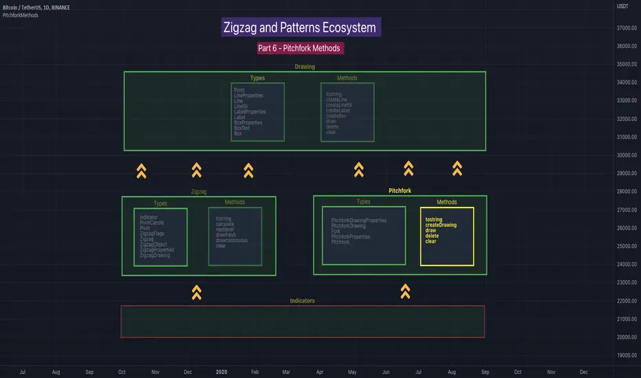
ZigzagMethodsLibrary "ZigzagMethods"
Object oriented implementation of Zigzag methods. Please refer to ZigzagTypes library for User defined types used in this library
tostring(this, sortKeys, sortOrder, includeKeys)
Converts ZigzagTypes/Pivot object to string representation
Parameters:
this : ZigzagTypes/Pivot
sortKeys : If set to true, string output is sorted by keys.
sortOrder : Applicable only if sortKeys is set to true. Positive number will sort them in ascending order whreas negative numer will sort them in descending order. Passing 0 will not sort the keys
includeKeys : Array of string containing selective keys. Optional parmaeter. If not provided, all the keys are considered
Returns: string representation of ZigzagTypes/Pivot
tostring(this, sortKeys, sortOrder, includeKeys)
Converts Array of Pivot objects to string representation
Parameters:
this : Pivot object array
sortKeys : If set to true, string output is sorted by keys.
sortOrder : Applicable only if sortKeys is set to true. Positive number will sort them in ascending order whreas negative numer will sort them in descending order. Passing 0 will not sort the keys
includeKeys : Array of string containing selective keys. Optional parmaeter. If not provided, all the keys are considered
Returns: string representation of Pivot object array
tostring(this)
Converts ZigzagFlags object to string representation
Parameters:
this : ZigzagFlags object
Returns: string representation of ZigzagFlags
tostring(this, sortKeys, sortOrder, includeKeys)
Converts ZigzagTypes/Zigzag object to string representation
Parameters:
this : ZigzagTypes/Zigzagobject
sortKeys : If set to true, string output is sorted by keys.
sortOrder : Applicable only if sortKeys is set to true. Positive number will sort them in ascending order whreas negative numer will sort them in descending order. Passing 0 will not sort the keys
includeKeys : Array of string containing selective keys. Optional parmaeter. If not provided, all the keys are considered
Returns: string representation of ZigzagTypes/Zigzag
calculate(this, ohlc, indicators, indicatorNames)
Calculate zigzag based on input values and indicator values
Parameters:
this : Zigzag object
ohlc : Array containing OHLC values. Can also have custom values for which zigzag to be calculated
indicators : Array of indicator values
indicatorNames : Array of indicator names for which values are present. Size of indicators array should be equal to that of indicatorNames
Returns: current Zigzag object
calculate(this)
Calculate zigzag based on properties embedded within Zigzag object
Parameters:
this : Zigzag object
Returns: current Zigzag object
nextlevel(this)
Calculate Next Level Zigzag based on the current calculated zigzag object
Parameters:
this : Zigzag object
Returns: Next Level Zigzag object
clear(this)
Clears zigzag drawings array
Parameters:
this : array
Returns: void
drawfresh(this)
draws fresh zigzag based on properties embedded in ZigzagDrawing object
Parameters:
this : ZigzagDrawing object
Returns: ZigzagDrawing object
drawcontinuous(this)
draws zigzag based on the zigzagmatrix input
Parameters:
this : ZigzagDrawing object
Returns:

PVSRA Volume Price - Some people say "Price Action is King". I say, we cannot know how the MMs (Market Makers) will move price next, period. But price tends to consolidate above key SR when MMs are filling short orders for SM (Smart Money) and long orders for DM (Dumb Money), and price tends to consolidate below key SR when MMs are filling long orders for SM and short orders for DM. The MMs are also "SM", and they tend to do the other SMs "one better"! This means that after the MMs fill the SM/DM orders, they might move price a bit further in an attempt to stop out some of those SM executed orders and sucker in more DM; both giving liquidity for the MMs to add to their own SM side position. Yes, the MMs are bastards. But the point is that could leave price not "nicely" above or below a SR anymore, yet more consolidation can occur.
Volume - Increases in activity denote increase in interest. But, is it long or short interest? Where is price in the bigger picture when this is happening? Is it at relative highs, or lows in the overall price action? And if a high volume bar is for a candle which you can examine by going to lower TF charts, you might see where in the spread of that candle the most volume occurred, high or low! Using volume is about taking note of relative increases in volume and what price is doing at the same time. Are the better volumes favoring the lower or the higher prices, as the MMs waffle price up and down? And do the volumes get particularly notable when the MMs take price above or below key SR?
S&R - Read all about S&R at "Baby Pips.com". What I want you to realize here is that the whole, half and quarter numbered price levels (hereinafter referred to as "Levels") are the most important SR of all in this market! Not because price stops, pauses, proceeds or reverses there, but because it is above or below these levels that important consolidation (MMs filling SM orders) takes place. Once SM long orders are filled, they become interested in placing orders to close them at higher prices, and hence the MMs will be moving price higher, eventually. Once SM short orders are filled, they become interested in placing orders to close them at lower prices, and hence the MMs will be moving price lower, eventually.
PVSRA - If we can spot consolidations above/below key SR, examine the overall price action on various TF charts, and take note of where the notable increases in volume have most recently occurred (did volume favor relative highs or lows), then we can build a consensus about what kind of orders the MMs have most recently been filling; buying to open longs or close shorts, or selling to open shorts or close longs. And we can get a better idea if things will next become bullish or bearish. And once PA confirms our bullish or bearish PVSRA results, by recognizing the importance of Levels we can look beyond current PA in the direction it is going and look to historic PA S&R (consolidation around key Levels) to come up with candidates for where the price might be headed. And bull or bear swings typically run in terms of 100+, 150+, 200+ pips, .....etc. And now you know why.
Okay. Now, if this is your first introduction to PVSRA, and having just read the above, you are likely scratching your head and still confused. That is normal. I will tell you a secret about the market and why you have a right to be confused. The secret is this. The market cannot be defined by mathematics nor by immutable logic. This is why the most advanced mathematicians over a century have never even come close to cracking the market. It cannot be done. Something else, other than math and immutable logic is the fundamental operand in the market. Have you ever watched a child attempt a jigsaw puzzle for the first time? And watched as that child grew and attempted more of them, and more complex ones? What is at work in the market I will elaborate on later, but for now trust me in this. We need to apply ourselves to learning how to do PVSRA just as a child attacks learning how to do jigsaw puzzles. And we must continue doing PVSRA, because in time our mind will "learn" when we have just picked up an important piece of the puzzle, and that we know where it goes! Developing the skill of PVSRA is an art form. We must not allow ourselves to feel badly if we miss clues. PVSRA is an art form that takes time to perfect. Over time our skill will grow and our "read" of the unpredictable market will improve. We must take to ongoing learning and application of PVSRA.
Introduction to How the Market Really Works
Does anybody remember the "lil' Abner" cartoons in the Sunday papers? Let me draw for you a mental picture of how the market really works.....
Imagine Daddy Yokum ferociously racing a buckboard wagon up and down the steep inclines and declines in the rough, rocky mountain road that has sharp turns and a sheer cliff on one side. The wagon wheels are spewing rocks off the side of the cliff! Even Daddy Yokum's shotgun is going off due to the jolting of the buckboard! Daddy Yokum has a demented look on his face, but he is smiling! The horse has a wild look in it's eyes and is frothing at the mouth. There are two passengers being tossed around in the back of the buckboard, terror stricken! Now, let's pan back from this cartoon picture and place the labels needed. On the side of the wagon is the sign "Market Pricing". The demented, smiling Daddy Yokum, is the Market Maker. The passengers being tossed around are the buyers and sellers.
.....Got it? Market prices are not determined by the buyers and sellers. They are determined by the Robber Bank Market Makers (MMs).
MMs are Market Manipulators of Price, and Thieves!
The "market" is the sole creation of the Robber Banks that "make the market". While it serves the world of commerce, they run it to make profits. And they opened the market up to foster prolific currency trading by others for the sole purpose of making more profits. They move prices up and down to "create liquidity" to fill the orders of SM (Smart Money) and DM (Dumb Money), for the commissions they make by filling the orders. When they have some orders above the current price and some below the current price, who do you think determines the sequence of direction and distance the price is going to move so these orders can be filled? And always - since they know how they are going to move price next - they take positions themselves to make additional profits.
They do this by:
1. Manipulating price to sucker into the market DM that is taking the wrong side position.
2. Manipulating price to sucker into the market SM that is taking the right side position, but too soon, and later manipulating price to hit their stops.
They have total control of pricing, and by these actions they effectively "steal" from others the money to fill their own "right side" positions before moving the price to the next area they have decided on for filling orders, and for taking profit on their positions built beforehand. Don't get me wrong. I do not object to the market volatility these thieving Robber Banks create. We need it. But we also need to understand what these people are like, the cloth they are cut from. They are crooks, and we have to be extra careful about trading in the market they operate. On some special days you can see them in their true colors. We should witness it. Take note of it. Speak of it. And remember it!

IIPThis indicator includes followings functions,
1. Close and SMA
Show 8 SMA (default: 3, 5, 7, 9, 20, 100, 300: each can be adjustable.)
2. Background color in Perfect Order (5, 20 ,60)
Perfect Order: Red
Reverse Perfect Order: Blue
3. Golden Cross and Dead Cross between SMA 5 and SMA 20
Golden Cross(GC):▲ with Green
Dead Cross(DC):▼ with Red
4. Show labels on 5 days, 20 days, 60 days and 100 days before today
5. Put dotted vertical line on first day in every month.
Doji swing strategyThis is a simple strategy based on Doji star candlestick
This strategy is suited for big time frames, like 4h -1Day and so on.
It places two orders: long at doji star high or previous candle high and short at doji star low or previous candle low.
It can also be applied volume average, in order to filter between trades .
This strategy works very well with high time frames like Weekly TF because it eliminates the noise in doji formation.
It also has inside a risk management made of SL/TP , or if not prefered it can exit based on a exit condition.
If you have any questions, please let me know !
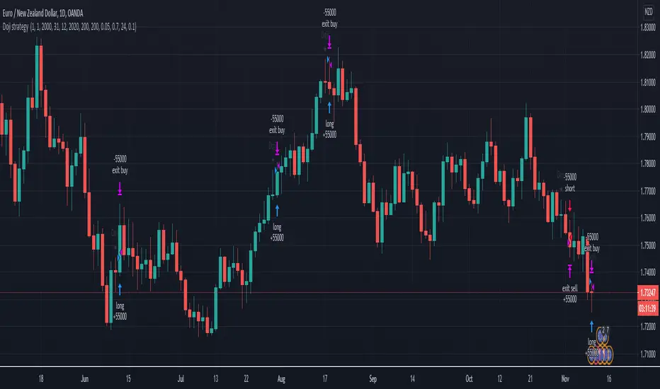
SB_CCI coded OBV StrategyStrategy-
Buy Order: Previous obv value is green and obv_cci coded line crosses over ema line
Sell Order: Previous obv value is red and obv_cci coded line crosses under ema line.
Original Idea:
Preferable for day/week intervals.
For Tips to continue :) -
BTC: 1BjswGcRR6c23pka7qh5t5k56j46cuyyy2
ETH: 0x64fed71c9d6c931639c7ba4671aeb6b05e6b3781
LTC: LKT2ykQ8QSzzfTDB6Tnsf12xwYPjgq95h4

BioSwarm Imprinter™BioSwarm Imprinter™ — Agent-Based Consensus for Traders
What it is
BioSwarm Imprinter™ is a non-repainting, agent-based sentiment oscillator. It fuses many short-to-medium lookback “opinions” into one 0–100 consensus line that is easy to read at a glance (50 = neutral, >55 bullish bias, <45 bearish bias). The engine borrows from swarm intelligence: many simple voters (agents) adapt their influence over time based on how well they’ve been predicting price, so the crowd gets smarter as conditions change.
Use it to:
• Detect emerging trends sooner without overreacting to noise.
• Filter mean-reversion vs continuation opportunities.
• Gate entries with a confidence score that reflects both strength and persistence of the move.
• Combine with your execution tools (VWAP/ORB/levels) as a state filter rather than a trade signal by itself.
⸻
Why it’s different
• Swarm learning: Each agent improves or decays its “fitness” depending on whether its vote matched the next bar’s direction. High-fitness agents matter more; weak agents fade.
• Multi-horizon by design: The crowd is composed of fixed, simple lookbacks spread from lenMin to lenMax. You get a blended, robust view instead of a single fragile parameter.
• Two complementary lenses: Each agent evaluates RSI-style balance (via Wilder’s RMA) and momentum (EMA deviation). You decide the weight of each.
• No repaint, no MTF pitfalls: Everything runs on the chart’s timeframe with bar-close confirmation; no request.security() or forward references.
• Actionable UI: A clean consensus line, optional regime background, confidence heat, and triangle markers when thresholds are crossed.
⸻
What you see on the chart
• Consensus line (0–100): Smoothed to your preference; color/area makes bull/bear zones obvious.
• Regime coloring (optional): Light green in bull zone, light red in bear zone; neutral otherwise.
• Confidence heat: A small gauge/number (0–100) that combines distance from neutral and recent persistence.
• Markers (optional): Triangles when consensus crosses up through your bull threshold (e.g., 55) or down through your bear threshold (e.g., 45).
• Info panel (optional): Consensus value, regime, confidence, number of agents, and basic diagnostics.
⸻
How it works (under the hood)
1. Horizon bins: The range is divided into numBins. Each bin has a fixed, simple integer length (crucial for Pine’s safety rules).
2. Per-bin features (computed every bar):
• RSI-style balance using Wilder’s RMA (not ta.rsi()), then mapped to −1…+1.
• Momentum as (close − EMA(L)) / EMA(L) (dimensionless drift).
3. Agent vote: For its assigned bin, an agent forms a weighted score: score = wRSI*RSI_like + wMOM*Momentum. A small dead-band near zero suppresses chop; votes are +1/−1/0.
4. Fitness update (bar close): If the agent’s previous vote agreed with the next bar’s direction, multiply its fitness by learnGain; otherwise by learnPain. Fitness is clamped so it never explodes or dies.
5. Consensus: Weighted average of all votes using fitness as weights → map to 0–100 and smooth with EMA.
Why it doesn’t repaint:
• No future references, no MTF resampling, fitness updates only on confirmed bars.
• All TA primitives (RMA/EMA/deltas) are computed every bar unconditionally.
⸻
Signals & confidence
• Bullish bias: consensus ≥ bullThr (e.g., 55).
• Bearish bias: consensus ≤ bearThr (e.g., 45).
• Confidence (0–100):
• Distance score: how far consensus is from 50.
• Momentum score: how strong the recent change is versus its recent average.
• Combined into a single gate; start filtering entries at ≥60 for higher quality.
Tip: For range sessions, raise thresholds (60/40) and increase smoothing; for momentum sessions, lower smoothing and keep thresholds at 55/45.
⸻
Inputs you’ll actually tune
• Agents & horizons:
• N_agents (e.g., 64–128)
• lenMin / lenMax (e.g., 6–30 intraday, 10–60 swing)
• numBins (e.g., 12–24)
• Weights & smoothing:
• wRSI vs wMOM (e.g., 0.7/0.3 for FX & indices; 0.6/0.4 for crypto)
• deadBand (0.03–0.08)
• consSmooth (3–8)
• Thresholds & hygiene:
• bullThr/bearThr (55/45 default)
• cooldownBars to avoid signal spam
⸻
Playbooks (ready-to-use)
1) Breakout / Trend continuation
• Timeframe: 15m–1h for day/swing.
• Filter: Take longs only when consensus > 55 and confidence ≥ 60.
• Execution: Use your ORB/VWAP/pullback trigger for entry. Trail with swing lows or 1.5×ATR. Exit on a close back under 50 or when a bearish signal prints.
2) Mean reversion (fade)
• When: Sideways days or low-volatility clusters.
• Setup: Increase deadBand and consSmooth.
• Signal: Bearish fades when consensus rolls over below ≈55 but stays above 50; bullish fades when it rolls up above ≈45 but stays below 50.
• Targets: The neutral zone (~50) as the first take-profit.
3) Multi-TF alignment
• Keep BioSwarm on 1H for bias, execute on 5–15m:
• Only take entries in the direction of the 1H consensus.
• Skip counter-bias scalps unless confidence is very low (explicit mean-reversion plan).
⸻
Integrations that work
• DynamoSent Pro+ (macro bias): Only act when macro bias and swarm consensus agree.
• ORB + Session VWAP Pro: Trade London/NY ORB breakouts that retest while consensus >55 (long) or <45 (short).
• Levels/Orderflow: BioSwarm is your “go / no-go”; execution stays with your usual triggers.
⸻
Quick start
1. Drop the indicator on a 1H chart.
2. Start with: N_agents=64, lenMin=6, lenMax=30, numBins=16, deadBand=0.06, consSmooth=5, thresholds 55/45.
3. Trade only when confidence ≥ 60.
4. Add your favorite execution tool (VWAP/levels/OR) for entries & exits.
⸻
Non-repainting & safety notes
• No request.security(); no hidden lookahead.
• Bar-close confirmation for fitness and signals.
• All TA calls are unconditional (no “sometimes called” warnings).
• No series-length inputs to RSI/EMA — we use RMA/EMA formulas that accept fixed simple ints per bin.
⸻
Known limits & tips
• Too many signals? Raise deadBand, increase consSmooth, widen thresholds to 60/40.
• Too few signals? Lower deadBand, reduce consSmooth, narrow thresholds to 53/47.
• Over-fitting risk: Keep learnGain/learnPain modest (e.g., ×1.04 / ×0.96).
• Compute load: Large N_agents × numBins is heavier; scale to your device.
⸻
Example recipes
EURUSD 1H (swing):
lenMin=8, lenMax=34, numBins=16, wRSI=0.7, wMOM=0.3, deadBand=0.06, consSmooth=6, thr=55/45
Buy breakouts when consensus >55 and confidence ≥60; confirm with 5–15m pullback to VWAP or level.
SPY 15m (US session):
lenMin=6, lenMax=24, numBins=12, consSmooth=4, deadBand=0.05
On trend days, stay with longs as long as consensus >55; add on shallow pullbacks.
BTC 1H (24/7):
Increase momentum weight: wRSI=0.6, wMOM=0.4, extend lenMax to ~50. Use dynamic stops (ATR) and partials on strong verticals.
⸻
Final word
BioSwarm is a state engine: it tells you when the market is primed to continue or mean-revert. Pair it with your entries and risk framework to turn that state into trades. If you’d like, I can supply a companion strategy template that consumes the consensus and back-tests the three playbooks (Breakout/Fade/Flip) with standard risk management.
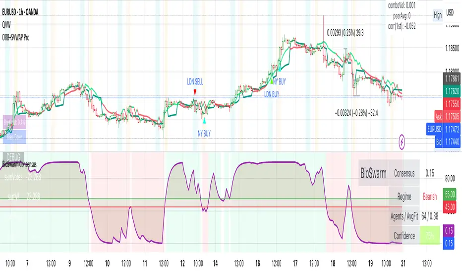
BK AK-Flag Formations🏴☠️ Introducing BK AK-Flag Formations — Raise the standard. Drive the line. Continue the assault. 🏴☠️
Built for traders who exploit momentum with discipline: flagpoles, flags, and pennants detected, tagged, and briefed—so you can press advantage instead of hesitating.
🎖️ Full Credit
The pattern engine, detection logic, and architecture are Trendoscope—one of the absolute best coders on TradingView and the original creator of this indicator’s core. I asked for interface upgrades and knew he was deep in other builds, so I forged the add-ons and released them for the community that values them.
My enhancements (on top of Trendoscope):
Label transparency (text + background)
Short-form labels (BF/BeF/BP/BeP/…)
Transparency controls for short-form labels
Hover tooltips with full pattern name + bullish/bearish bias (toggle)
Everything else is Trendoscope. Respect where it’s due.
🧠 What It Does
Locks onto flags and pennants after strong impulses (flagpoles).
Prints clean battlefield tags (BF, BeF, BP, BeP…) so the setup is obvious without burying price.
Mouse-over for the brief: full pattern name + directional bias exactly when you need it.
Multi-zigzag sweep for micro→macro detection, overlap control, bar-ratio verification, max-pattern caps, dark/light aware palette + custom colors.
🧭 Read the Continuation
BF — Bull Flag: strong pole, orderly pullback; look for break and measured move continuity.
BP — Bull Pennant: tight triangle after thrust; expansion confirms carry.
BeF — Bear Flag: weak rallies in a downtrend; break = continuation lower.
BeP — Bear Pennant: compressed pause beneath resistance; release favors trend.
Standards are not decoration—they are orders.
🤝 Acknowledgments
Original engine & libraries: Trendoscope (legend).
Enhancement layer (UX): transparency, short codes, tooltip system — BK.
Mentor: A.K. — clarity, patience, judgment. His discipline guides every choice here.
🫡 Give Forward
Don’t be cheap with your knowledge. If my indicators sharpen your edge:
Teach someone to read structure with discipline.
Share your process, not just screenshots.
Contribute code, context, or courage to those behind you.
Tools are force multipliers. Character decides how they’re used.
🙏 Final Word
“Plans are established by counsel; by wise guidance wage war.” — Proverbs 20:18
Impulse → formation → continuation.
Raise the banner, hold formation, and execute with wisdom.
BK AK-Flag Formations — when the standard rises, the line advances.
Gd bless. 🙏
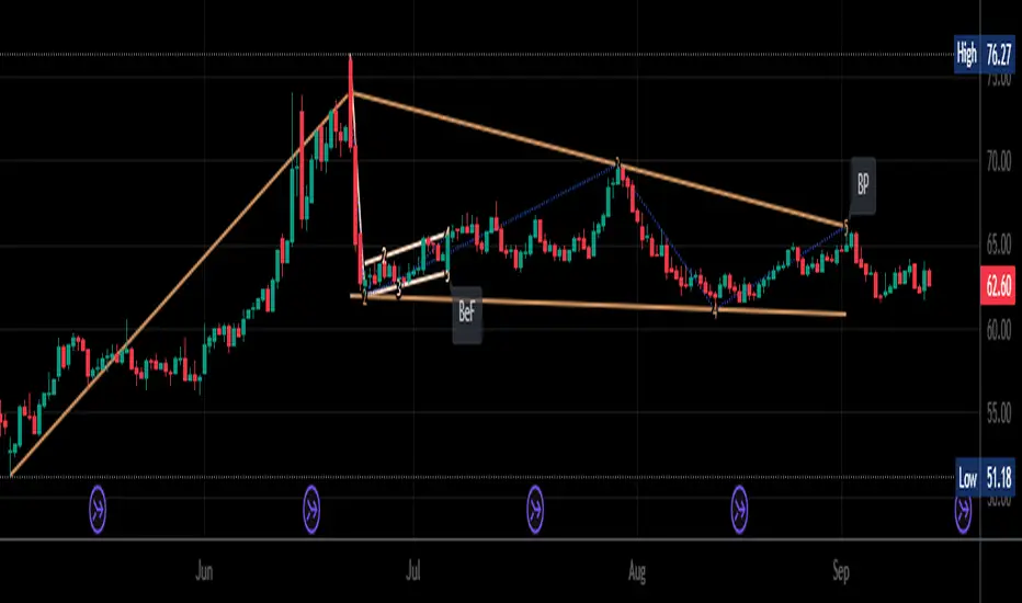
EMA20 Cross Strategy with countertrades and signalsEMA20 Cross Strategy Documentation
Overview
The EMA20 Cross Strategy with Counter-Trades and Instant Signals is a Pine Script (version 6) trading strategy designed for the TradingView platform. It implements an Exponential Moving Average (EMA) crossover system to generate buy and sell signals, with optional trend filtering, session-based trading, instant signal processing, and visual/statistical feedback. The strategy supports counter-trades (closing opposing positions before entering new ones) and operates with a fixed trade size in EUR.
Features
EMA Crossover Mechanism:
Uses a short-term EMA (configurable length, default: 1) and a long-term EMA (default: 20) to detect crossovers.
A buy signal is generated when the short EMA crosses above the long EMA.
A sell signal is generated when the short EMA crosses below the long EMA.
Instant Signals:
If enabled (useInstantSignals), signals are based on the current price crossing the short EMA, rather than waiting for the candle close.
This allows faster trade execution but may increase sensitivity to price fluctuations.
Trend Filter:
Optionally filters trades based on the trend direction (useTrendFilter).
Long trades are allowed only when the short EMA (or price, for instant signals) is above the long EMA.
Short trades are allowed only when the short EMA (or price) is below the long EMA.
Session Filter:
Restricts trading to specific market hours (sessionStart, default: 09:00–17:00) if enabled (useSessionFilter).
Ensures trades occur only during active market sessions, reducing exposure to low-liquidity periods.
Customizable Timeframe:
The EMA calculations can use a higher timeframe (e.g., 5m, 15m, 1H, 4H, 1D, default: 1H) via request.security.
This allows the strategy to base signals on longer-term trends while operating on a shorter-term chart.
Trade Management:
Fixed trade size of €100,000 per trade (tradeAmount), with a maximum quantity cap (maxQty = 10,000) to prevent oversized trades.
Counter-trades: Closes short positions before entering a long position and vice versa.
Trades are executed with a minimum quantity of 1 to ensure valid orders.
Visualization:
EMA Lines: The short EMA is colored based on the last signal (green for buy, red for sell, gray for neutral), and the long EMA is orange.
Signal Markers: Displays buy/sell signals as arrows (triangles) above/below candles if enabled (showSignalShapes).
Background/Candle Coloring: Optionally colors the chart background or candles green (bullish) or red (bearish) based on the trend (useColoredBars).
Statistics Display:
If enabled (useStats), a label on the chart shows:
Total closed trades
Open trades
Win rate (%)
Number of winning/losing trades
Profit factor (gross profit / gross loss)
Net profit
Maximum drawdown
Configuration Inputs
EMA Short Length (emaLength): Length of the short-term EMA (default: 1).
Trend EMA Length (trendLength): Length of the long-term EMA (default: 20).
Enable Trend Filter (useTrendFilter): Toggles trend-based filtering (default: true).
Color Candles (useColoredBars): Colors candles instead of the background (default: true).
Enable Session Filter (useSessionFilter): Restricts trading to specified hours (default: false).
Trading Session (sessionStart): Defines trading hours (default: 09:00–17:00).
Show Statistics (useStats): Displays performance stats on the chart (default: true).
Show Signal Arrows (showSignalShapes): Displays buy/sell signals as arrows (default: true).
Use Instant Signals (useInstantSignals): Generates signals based on live price action (default: false).
EMA Timeframe (emaTimeframe): Timeframe for EMA calculations (options: 5m, 15m, 1H, 4H, 1D; default: 1H).
Strategy Logic
Signal Generation:
Standard Mode: Signals are based on EMA crossovers (short EMA crossing long EMA) at candle close.
Instant Mode: Signals are based on the current price crossing the short EMA, enabling faster reactions.
Trade Execution:
On a buy signal, closes any short position and opens a long position.
On a sell signal, closes any long position and opens a short position.
Position size is calculated as the minimum of €100,000 or available equity, divided by the current price, capped at 10,000 units.
Filters:
Trend Filter: Ensures trades align with the trend direction (if enabled).
Session Filter: Restricts trades to user-defined market hours (if enabled).
Visual Feedback
EMA Lines: Provide a clear view of the short and long EMAs, with the short EMA’s color reflecting the latest signal.
Signal Arrows: Large green triangles (buy) below candles or red triangles (sell) above candles for easy signal identification.
Chart Coloring: Highlights bullish (green) or bearish (red) trends via background or candle colors.
Statistics Label: Displays key performance metrics in a label above the chart for quick reference.
Usage Notes
Initial Capital: €100,000 (configurable via initial_capital).
Currency: EUR (set via currency).
Order Processing: Orders are processed at candle close (process_orders_on_close=true) unless instant signals are enabled.
Dynamic Requests: Allows dynamic timeframe adjustments for EMA calculations (dynamic_requests=true).
Platform: Designed for TradingView, compatible with any market supported by the platform (e.g., stocks, forex, crypto).
Example Use Case
Scenario: Trading on a 5-minute chart with a 1-hour EMA timeframe, trend filter enabled, and session filter set to 09:00–17:00.
Behavior: The strategy will:
Calculate EMAs on the 1-hour timeframe.
Generate buy signals when the short EMA crosses above the long EMA (and price is above the long EMA).
Generate sell signals when the short EMA crosses below the long EMA (and price is below the long EMA).
Execute trades only during 09:00–17:00.
Display green/red candles and performance stats on the chart.
Limitations
Instant Signals: May lead to more frequent signals, increasing the risk of false positives in volatile markets.
Fixed Trade Size: Does not adjust dynamically based on market conditions beyond equity and max quantity limits.
Session Filter: Simplified and may not account for complex session rules or holidays.
Statistics: Displayed on-chart, which may clutter the view in smaller charts.
Customization
Adjust emaLength and trendLength to suit different market conditions (e.g., shorter for scalping, longer for swing trading).
Toggle useInstantSignals for faster or more stable signal generation.
Modify sessionStart to align with specific market hours.
Disable useStats or showSignalShapes for a cleaner chart.
This strategy is versatile for both manual and automated trading, offering flexibility for various markets and trading styles while providing clear visual and statistical feedback.
Simple Liquidity Zones [Supertrade]🔎 What this indicator does
This indicator is designed to highlight liquidity sweep zones on the chart.
• A liquidity sweep occurs when price briefly breaks above a recent swing high or below a recent swing low, but fails to close beyond it.
• Such behavior often indicates that price has taken liquidity (stop orders resting above highs or below lows) and may reverse.
The indicator marks these events as bullish or bearish liquidity zones:
• Bullish Zone (green) → Price swept a swing low and closed back above it (possible bullish reversal area).
• Bearish Zone (red) → Price swept a swing high and closed back below it (possible bearish reversal area).
These zones are drawn as shaded horizontal bands that extend forward in time, providing visual areas where liquidity grabs occurred.
________________________________________
⚙️ How calculations are made
The indicator does not use moving averages or smoothing.
Instead, it works with raw price action:
1. Swing Detection → It checks the highest high and lowest low of the past N bars (swing length).
2. Sweep Logic →
o A bearish sweep happens if the high breaks above the previous swing high, but the close returns below that level.
o A bullish sweep happens if the low breaks below the previous swing low, but the close returns above that level.
3. Zone Creation → When a sweep is detected, a shaded zone is drawn just above/below the swing level.
4. Persistence → Zones extend into the future until replaced by new ones (or optionally until price fully trades through them).
This makes the calculations simple, transparent, and responsive to actual market structure without lag.
________________________________________
📈 How it helps traders
This tool helps traders by:
• Visualizing liquidity areas → Shows where price previously swept liquidity and may act as support/resistance.
• Identifying reversals → Helps spot potential turning points after liquidity grabs.
• Risk management → Zones highlight areas where stops may be targeted, useful for positioning stop-loss orders.
• Confluence tool → Works best when combined with other strategies such as order blocks, trendlines, or volume analysis.
⚠️ Note: Like all indicators, this should not be used in isolation. It provides context, not guaranteed trade signals.
________________________________________
🏦 Markets & Timeframes
• Works across all markets (crypto, forex, stocks, indices, commodities).
• Particularly effective in high-liquidity environments where stop-hunting is common (e.g., forex majors, BTC/ETH, S&P500).
• Timeframes:
o Lower timeframes (1m–15m) → Scalpers can spot intraday liquidity sweeps.
o Higher timeframes (1H–1D) → Swing traders can identify major liquidity pools.
________________________________________