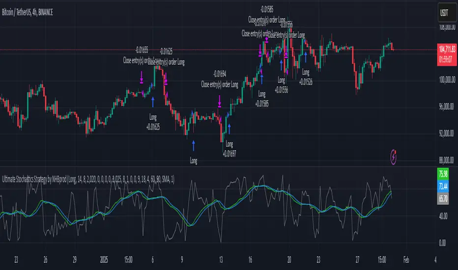
Ultimate Stochastics Strategy by NHBprod Use to Day Trade BTCHey All!
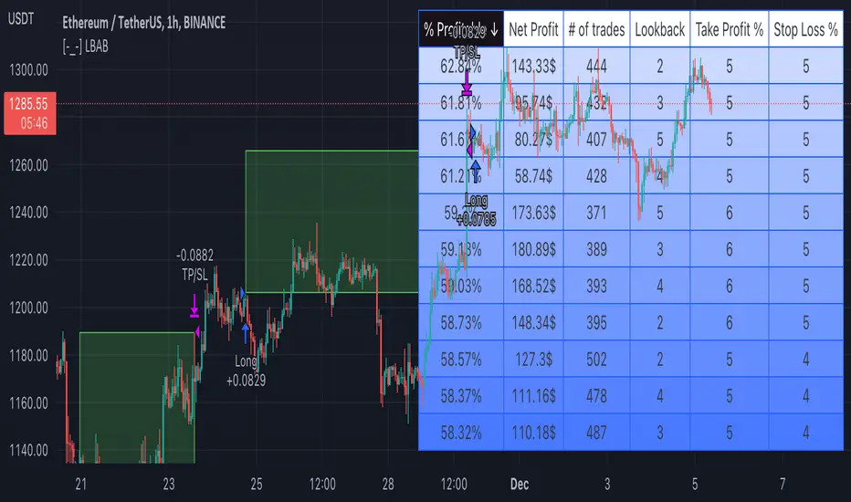
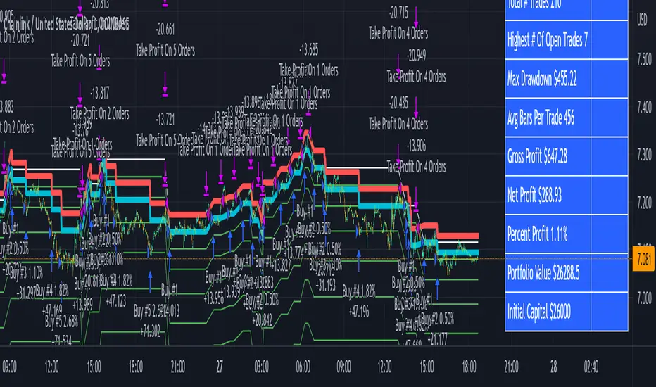
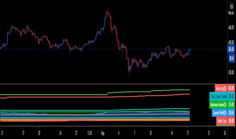
Here's a new script I worked on that's super simple but at the same time useful. Check out the backtest results. The backtest results include slippage and fees/commission, and is still quite profitable. Obviously the profitability magnitude depends on how much capital you begin with, and how much the user utilizes per order, but in any event it seems to be profitable according to backtests.
This is different because it allows you full functionality over the stochastics calculations which is designed for random datasets. This script allows you to:
Designate ANY period of time to analyze and study
Choose between Long trading, short trading, and Long & Short trading
It allows you to enter trades based on the stochastics calculations
It allows you to EXIT trades using the stochastics calculations or take profit, or stop loss, Or any combination of those, which is nice because then the user can see how one variable effects the overall performance.
As for the actual stochastics formula, you get control, and get to SEE the plot lines for slow K, slow D, and fast K, which is usually not considered.
You also get the chance to modify the smoothing method, which has not been done with regular stochastics indicators. You get to choose the standard simple moving average (SMA) method, but I also allow you to choose other MA's such as the HMA and WMA.
Lastly, the user gets the option of using a custom trade extender, which essentially allows a buy or sell signal to exist for X amount of candles after the initial signal. For example, you can use "max bars since signal" to 1, and this will allow the indicator to produce an extra sequential buy signal when a buy signal is generated. This can be useful because it is possible that you use a small take profit (TP) and quickly exit a profitable trade. With the max bars since signal variable, you're able to reenter on the next candle and allow for another opportunity.
Let me know if you have any questions! Please take a look at the performance report and let me know your thoughts! :)
Strategi Pine Script®