SMA Crossover with RSI ConfirmationThis is a sniper entry indicator that provides Buy and Sell signals using other Indicators to give the best possible Entries
Moving Average Crossovers:
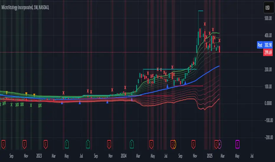
The indicator uses two moving averages: a short-term SMA (Simple Moving Average) and a long-term SMA.
When the short-term SMA crosses above the long-term SMA, it generates a buy signal (indicating potential upward momentum).
When the short-term SMA crosses below the long-term SMA, it generates a sell signal (indicating potential downward momentum).
RSI Confirmation:
The indicator incorporates RSI (Relative Strength Index) to confirm the buy and sell signals generated by the moving average crossovers.
RSI is used to gauge the overbought and oversold conditions of the market.
A buy signal is confirmed if RSI is below a specified overbought level, indicating potential buying opportunity.
A sell signal is confirmed if RSI is above a specified oversold level, indicating potential selling opportunity.
Dynamic Take Profit and Stop Loss:
The indicator calculates dynamic take profit and stop loss levels based on the Average True Range (ATR).
ATR is used to gauge market volatility, and the take profit and stop loss levels are adjusted accordingly.
This feature helps traders to manage their risk effectively by setting appropriate profit targets and stop loss levels.
Combining the information provided by these, the indicator will provide an entry point with a provided take profit and stop loss. The indicator can be applied to different asset classes. Risk management must be applied when using this indicator as it is not 100% guaranteed to be profitable.
Penunjuk Pine Script®