Keltner Channel Strategy by Kevin DaveyKeltner Channel Strategy Description
The Keltner Channel Strategy is a volatility-based trading approach that uses the Keltner Channel, a technical indicator derived from the Exponential Moving Average (EMA) and Average True Range (ATR). The strategy helps identify potential breakout or mean-reversion opportunities in the market by plotting upper and lower bands around a central EMA, with the channel width determined by a multiplier of the ATR.
Components:
1. Exponential Moving Average (EMA):
The EMA smooths price data by placing greater weight on recent prices, allowing traders to track the market’s underlying trend more effectively than a simple moving average (SMA). In this strategy, a 20-period EMA is used as the midline of the Keltner Channel.
2. Average True Range (ATR):
The ATR measures market volatility over a 14-period lookback. By calculating the average of the true ranges (the greatest of the current high minus the current low, the absolute value of the current high minus the previous close, or the absolute value of the current low minus the previous close), the ATR captures how much an asset typically moves over a given period.
3. Keltner Channel:
The upper and lower boundaries are set by adding or subtracting 1.5 times the ATR from the EMA. These boundaries create a dynamic range that adjusts with market volatility.
Trading Logic:
• Long Entry Condition: The strategy enters a long position when the closing price falls below the lower Keltner Channel, indicating a potential buying opportunity at a support level.
• Short Entry Condition: The strategy enters a short position when the closing price exceeds the upper Keltner Channel, signaling a potential selling opportunity at a resistance level.
The strategy plots the upper and lower Keltner Channels and the EMA on the chart, providing a visual representation of support and resistance levels based on market volatility.
Scientific Support for Volatility-Based Strategies:
The use of volatility-based indicators like the Keltner Channel is supported by numerous studies on price momentum and volatility trading. Research has shown that breakout strategies, particularly those leveraging volatility bands such as the Keltner Channel or Bollinger Bands, can be effective in capturing trends and reversals in both trending and mean-reverting markets  .
Who is Kevin Davey?
Kevin Davey is a highly respected algorithmic trader, author, and educator, known for his systematic approach to building and optimizing trading strategies. With over 25 years of experience in the markets, Davey has earned a reputation as an expert in quantitative and rule-based trading. He is particularly well-known for winning several World Cup Trading Championships, where he consistently demonstrated high returns with low risk.
Cari dalam skrip untuk "range"

Williams %R StrategyThe Williams %R Strategy implemented in Pine Script™ is a trading system based on the Williams %R momentum oscillator. The Williams %R indicator, developed by Larry Williams in 1973, is designed to identify overbought and oversold conditions in a market, helping traders time their entries and exits effectively (Williams, 1979). This particular strategy aims to capitalize on short-term price reversals in the S&P 500 (SPY) by identifying extreme values in the Williams %R indicator and using them as trading signals.
Strategy Rules:
Entry Signal:
A long position is entered when the Williams %R value falls below -90, indicating an oversold condition. This threshold suggests that the market may be near a short-term bottom, and prices are likely to reverse or rebound in the short term (Murphy, 1999).
Exit Signal:
The long position is exited when:
The current close price is higher than the previous day’s high, or
The Williams %R indicator rises above -30, indicating that the market is no longer oversold and may be approaching an overbought condition (Wilder, 1978).
Technical Analysis and Rationale:
The Williams %R is a momentum oscillator that measures the level of the close relative to the high-low range over a specific period, providing insight into whether an asset is trading near its highs or lows. The indicator values range from -100 (most oversold) to 0 (most overbought). When the value falls below -90, it indicates an oversold condition where a reversal is likely (Achelis, 2000). This strategy uses this oversold threshold as a signal to initiate long positions, betting on mean reversion—an established principle in financial markets where prices tend to revert to their historical averages (Jegadeesh & Titman, 1993).
Optimization and Performance:
The strategy allows for an adjustable lookback period (between 2 and 25 days) to determine the range used in the Williams %R calculation. Empirical tests show that shorter lookback periods (e.g., 2 days) yield the most favorable outcomes, with profit factors exceeding 2. This finding aligns with studies suggesting that shorter timeframes can effectively capture short-term momentum reversals (Fama, 1970; Jegadeesh & Titman, 1993).
Scientific Context:
Mean Reversion Theory: The strategy’s core relies on mean reversion, which suggests that prices fluctuate around a mean or average value. Research shows that such strategies, particularly those using oscillators like Williams %R, can exploit these temporary deviations (Poterba & Summers, 1988).
Behavioral Finance: The overbought and oversold conditions identified by Williams %R align with psychological factors influencing trading behavior, such as herding and panic selling, which often create opportunities for price reversals (Shiller, 2003).
Conclusion:
This Williams %R-based strategy utilizes a well-established momentum oscillator to time entries and exits in the S&P 500. By targeting extreme oversold conditions and exiting when these conditions revert or exceed historical ranges, the strategy aims to capture short-term gains. Scientific evidence supports the effectiveness of short-term mean reversion strategies, particularly when using indicators sensitive to momentum shifts.
References:
Achelis, S. B. (2000). Technical Analysis from A to Z. McGraw Hill.
Fama, E. F. (1970). Efficient Capital Markets: A Review of Theory and Empirical Work. The Journal of Finance, 25(2), 383-417.
Jegadeesh, N., & Titman, S. (1993). Returns to Buying Winners and Selling Losers: Implications for Stock Market Efficiency. The Journal of Finance, 48(1), 65-91.
Murphy, J. J. (1999). Technical Analysis of the Financial Markets: A Comprehensive Guide to Trading Methods and Applications. New York Institute of Finance.
Poterba, J. M., & Summers, L. H. (1988). Mean Reversion in Stock Prices: Evidence and Implications. Journal of Financial Economics, 22(1), 27-59.
Shiller, R. J. (2003). From Efficient Markets Theory to Behavioral Finance. Journal of Economic Perspectives, 17(1), 83-104.
Williams, L. (1979). How I Made One Million Dollars… Last Year… Trading Commodities. Windsor Books.
Wilder, J. W. (1978). New Concepts in Technical Trading Systems. Trend Research.
This explanation provides a scientific and evidence-based perspective on the Williams %R trading strategy, aligning it with fundamental principles in technical analysis and behavioral finance.

Parent Session Sweeps + Alert Killzone Ranges with Parent Session Sweep
Key Features:
1. Multiple Session Support: The script tracks three major trading sessions - Asia, London, and New York. Users can customize the timing of these sessions.
2. Killzone Visualization: The strategy visually represents each session's range, either as filled boxes or lines, allowing traders to easily identify key price levels.
3. Parent Session Logic: The core of the strategy revolves around identifying a "parent" session - a session that encompasses the range of the following session. This parent session becomes the basis for potential trade setups.
4. Sweep and Reclaim Setups: The strategy looks for price movements that sweep (break above or below) the parent session's high or low, followed by a reclaim of that level. This price action often indicates a potential reversal.
5. Risk-Reward Filtering: Each potential setup is evaluated based on a user-defined minimum risk-reward ratio, ensuring that only high-quality trade opportunities are considered.
6. Candle Close Filter: An optional filter that checks the characteristics of the candle that reclaims the parent session level, adding an extra layer of confirmation to the setup.
7. Performance Tracking: The strategy keeps track of bullish and bearish setup success rates, providing valuable feedback on its performance over time.
8. Visual Aids: The script draws lines to mark the parent session's high and low, making it easy for traders to identify key levels.
How It Works:
1. The script continuously monitors price action across the defined sessions.
2. When a session fully contains the range of the next session, it's identified as a potential parent session.
3. The strategy then waits for price to sweep either the high or low of this parent session.
4. If a sweep occurs, it looks for a reclaim of the swept level within the parameters set by the user.
5. If a valid setup is identified, the script generates an alert and places a trade (if backtesting or running live).
6. The strategy continues to monitor the trade for either reaching the target (opposite level of the parent session) or hitting the stop loss.
Considerations for Signals:
- Sweep: A break of the parent session's high or low.
- Reclaim: A close back inside the parent session range after a sweep.
- Candle Characteristics: Optional filter for the reclaim candle (e.g., bullish candle for long setups).
- Risk-Reward: Each setup must meet or exceed the user-defined minimum risk-reward ratio.
- Session Timing: The strategy is sensitive to the defined session times, which should be set according to the trader's preferred time zone.
This strategy aims to capitalize on institutional order flow and liquidity patterns in the forex market, providing traders with a systematic approach to identifying potential reversal points with favorable risk-reward profiles.

Neural Momentum StrategyThis strategy combines Exponential Moving Average (EMA) analysis with a multi-timeframe approach. It uses a neural scoring system to evaluate market momentum and generate precise trading signals. The strategy is implemented in Pine Script v5 and is designed for use on TradingView.
Key Components
The strategy utilizes short-term (10-period) and long-term (25-period) EMAs. It calculates the difference between these EMAs to assess trend direction and strength. A neural scoring system evaluates EMA crossovers (weight: 12 points), trend strength (weight: 10 points), and price acceleration (weight: 4 points). The system implements a score smoothing algorithm using a 10-period EMA.
Multi-timeframe Analysis
The strategy automatically selects a higher timeframe based on the current chart timeframe. It calculates scores for both the current and higher timeframes, then combines these scores using a weighted average. The higher timeframe factor ranges from 3 to 6, depending on the current timeframe.
Trading Logic
Entry occurs when the final combined score turns positive after a change. Exit happens when the final combined score turns negative after a change. The strategy recalculates scores on each bar, ensuring responsive trading decisions.
Risk Management
An optional adaptive stop-loss system based on Average True Range (ATR) is available. The default ATR period is 10, and the stop factor is 1.2. Stop levels are dynamically adjusted on the higher timeframe.
Customization Options
Users can adjust EMA periods, signal line period, scoring weights, and enable/disable multi-timeframe analysis. The strategy allows setting specific date ranges for backtesting and deployment.
Position Sizing
The strategy uses a percentage-of-equity position sizing method, with a default of 30% of account equity per trade.
Code Structure
The strategy is built using TradingView's strategy framework. It employs efficient use of the request.security() function for multi-timeframe analysis. The main calculation function, calculate_score(), computes the neural score based on EMA differences and acceleration.
Performance Considerations
The strategy adapts to various market conditions through its multi-faceted scoring system. Multi-timeframe analysis helps filter out noise and identify stronger trends. The neural scoring approach aims to capture subtle market dynamics often missed by traditional indicators.
Limitations
Performance may vary across different markets and timeframes. The strategy's effectiveness relies on proper calibration of its numerous parameters. Users should thoroughly backtest and forward test before live implementation.
To summarize, the Neural Momentum Strategy represents a sophisticated approach to market analysis. It combines traditional technical indicators with advanced scoring techniques and multi-timeframe analysis. This strategy is designed for traders seeking a data-driven and adaptive method. It aims to identify high-probability trading opportunities across various market conditions.
This Neural Momentum Strategy is for informational and educational purposes only. It should not be considered financial advice. The strategy may exhibit slight repainting behavior due to the nature of multi-timeframe analysis and the use of the request.security() function. Historical values might change as new data becomes available.
Trading carries a high level of risk, and may not be suitable for all investors. Before deciding to trade, you should carefully consider your investment objectives, level of experience, and risk appetite. The possibility exists that you could sustain a loss of some or all of your initial investment. Therefore, you should not invest money that you cannot afford to lose.
Past performance is not indicative of future results. The author and TradingView are not responsible for any losses incurred as a result of using this strategy. Always exercise caution when using this or any trading strategy, and thoroughly test it before implementing in live trading scenarios.
Users are solely responsible for any trading decisions they make based on this strategy. It is strongly recommended that you seek advice from an independent financial advisor if you have any doubts.

QuantBuilder | FractalystWhat's the strategy's purpose and functionality?
QuantBuilder is designed for both traders and investors who want to utilize mathematical techniques to develop profitable strategies through backtesting on historical data.
The primary goal is to develop profitable quantitive strategies that not only outperform the underlying asset in terms of returns but also minimize drawdown.
For instance, consider Bitcoin (BTC), which has experienced significant volatility, averaging an estimated 200% annual return over the past decade, with maximum drawdowns exceeding -80%. By employing this strategy with diverse entry and exit techniques, users can potentially seek to enhance their Compound Annual Growth Rate (CAGR) while managing risk to maintain a lower maximum drawdown.
While this strategy employs quantitative techniques, including mathematical methods such as probabilities and positive expected values, it demonstrates exceptional efficacy across all markets. It particularly excels in futures, indices, stocks, cryptocurrencies, and commodities, leveraging their inherent trending behaviors for optimized performance.
In both trending and consolidating market conditions, QuantBuilder employs a combination of multi-timeframe probabilities, expected values, directional biases, moving averages and diverse entry models to identify and capitalize on bullish market movements.
How does the strategy perform for both investors and traders?
The strategy has two main modes, tailored for different market participants: Traders and Investors.
1. Trading:
- Designed for traders looking to capitalize on bullish markets.
- Utilizes a percentage risk per trade to manage risk and optimize returns.
- Suitable for both swing and intraday trading with a focus on probabilities and risk per trade approach.
2. Investing:
- Geared towards investors who aim to capitalize on bullish trending markets without using leverage while mitigating the asset's maximum drawdown.
- Utilizes pre-define percentage of the equity to buy, hold, and manage the asset.
- Focuses on long-term growth and capital appreciation by fully/partially investing in the asset during bullish conditions.
How does the strategy identify market structure? What are the underlying calculations?
The strategy utilizes an efficient logic with for loops to pinpoint the first swing candle featuring a pivot of 2, establishing the point at which the break of structure begins.
What entry criteria are used in this script? What are the underlying calculations?
The script utilizes two entry models: BreakOut and fractal.
Underlying Calculations:
Breakout: The script assigns the most recent swing high to a variable. When the price closes above this level and all other conditions are met, the script executes a breakout entry (conservative approach).
Fractal: The script identifies a swing low with a period of 2. Once this condition is met, the script executes the trade (aggressive approach).
How does the script calculate probabilities? What are the underlying calculations?
The script calculates probabilities by monitoring price interactions with liquidity levels. Here’s how the underlying calculations work:
Tracking Price Hits: The script counts the number of times the price taps into each liquidity side after the EQM level is activated. This data is stored in an array for further analysis.
Sample Size Consideration: The total number of price interactions serves as the sample size for calculating probabilities.
Probability Calculation: For each liquidity side, the script calculates the probability by taking the average of the recorded hits. This allows for a dynamic assessment of the likelihood that a particular side will be hit next, based on historical performance.
Dynamic Adjustment: As new price data comes in, the probabilities are recalculated, providing real-time aduptive insights into market behavior.
Note: The calculations are performed independently for each directional range. A range is considered bearish if the previous breakout was through a sellside liquidity. Conversely, a range is considered bullish if the most recent breakout was through a buyside liquidity.
How does the script calculate expected values? What are the underlying calculations?
The script calculates expected values by leveraging the probabilities of winning and losing trades, along with their respective returns. The process involves the following steps:
This quantitative methodology provides a robust framework for assessing the expected performance of trading strategies based on historical data and backtesting results.
How is the contextual bias calculated? What are the underlying calculations?
The contextual bias in the QuantBuilder script is calculated through a structured approach that assesses market structure based on swing highs and lows. Here’s how it works:
Identification of Swing Points: The script identifies significant swing points using a defined pivot logic, focusing on the first swing high and swing low. This helps establish critical levels for determining market structure.
Break of Structure (BOS) Assessment:
Bullish BOS: The script recognizes a bullish break of structure when a candle closes above the first swing high, followed by at least one swing low.
Bearish BOS: Conversely, a bearish break of structure is identified when a candle closes below the first swing low, followed by at least one swing high.
Bias Assignment: Based on the identified break of structure, the script assigns directional biases:
A bullish bias is assigned if a bullish BOS is confirmed.
A bearish bias is assigned if a bearish BOS is confirmed.
Quantitative Evaluation: Each identified bias is quantitatively evaluated, allowing the script to assign numerical values representing the strength of each bias. This quantification aids in assessing the reliability of market sentiment across multiple timeframes.
What's the purpose of using moving averages in this strategy? What are the underlying calculations?
Using moving averages is a widely-used technique to trade with the trend.
The main purpose of using moving averages in this strategy is to filter out bearish price action and to only take trades when the price is trading ABOVE specified moving averages.
The script uses different types of moving averages with user-adjustable timeframes and periods/lengths, allowing traders to try out different variations to maximize strategy performance and minimize drawdowns.
By applying these calculations, the strategy effectively identifies bullish trends and avoids market conditions that are not conducive to profitable trades.
The MA filter allows traders to choose whether they want a specific moving average above or below another one as their entry condition.
What type of stop-loss identification method are used in this strategy? What are the underlying calculations?
- Initial Stop-loss:
1. ATR Based:
The Average True Range (ATR) is a method used in technical analysis to measure volatility. It is not used to indicate the direction of price but to measure volatility, especially volatility caused by price gaps or limit moves.
Calculation:
- To calculate the ATR, the True Range (TR) first needs to be identified. The TR takes into account the most current period high/low range as well as the previous period close.
The True Range is the largest of the following:
- Current Period High minus Current Period Low
- Absolute Value of Current Period High minus Previous Period Close
- Absolute Value of Current Period Low minus Previous Period Close
- The ATR is then calculated as the moving average of the TR over a specified period. (The default period is 14)
2. ADR Based:
The Average Day Range (ADR) is an indicator that measures the volatility of an asset by showing the average movement of the price between the high and the low over the last several days.
Calculation:
- To calculate the ADR for a particular day:
- Calculate the average of the high prices over a specified number of days.
- Calculate the average of the low prices over the same number of days.
- Find the difference between these average values.
- The default period for calculating the ADR is 14 days. A shorter period may introduce more noise, while a longer period may be slower to react to new market movements.
3. PL Based:
This method places the stop-loss at the low of the previous candle.
If the current entry is based on the hunt entry strategy, the stop-loss will be placed at the low of the candle that wicks through the lower FRMA band.
Example:
If the previous candle's low is 100, then the stop-loss will be set at 100.
This method ensures the stop-loss is placed just below the most recent significant low, providing a logical and immediate level for risk management.
- Trailing Stop-Loss:
One of the key elements of this strategy is its ability to detect structural liquidity and structural invalidation levels across multiple timeframes to trail the stop-loss once the trade is in running profits.
By utilizing this approach, the strategy allows enough room for price to run.
By using these methods, the strategy dynamically adjusts the initial stop-loss based on market volatility, helping to protect against adverse price movements while allowing for enough room for trades to develop.
Each market behaves differently across various timeframes, and it is essential to test different parameters and optimizations to find out which trailing stop-loss method gives you the desired results and performance.
What type of break-even and take profit identification methods are used in this strategy? What are the underlying calculations?
For Break-Even:
Percentage (%) Based:
Moves the initial stop-loss to the entry price when the price reaches a certain percentage above the entry.
Calculation:
Break-even level = Entry Price * (1 + Percentage / 100)
Example:
If the entry price is $100 and the break-even percentage is 5%, the break-even level is $100 * 1.05 = $105.
Risk-to-Reward (RR) Based:
Moves the initial stop-loss to the entry price when the price reaches a certain RR ratio.
Calculation:
Break-even level = Entry Price + (Initial Risk * RR Ratio)
For TP1 (Take Profit 1):
- You can choose to set a take profit level at which your position gets fully closed or 50% if the TP2 boolean is enabled.
- Similar to break-even, you can select either a percentage (%) or risk-to-reward (RR) based take profit level, allowing you to set your TP1 level as a percentage amount above the entry price or based on RR.
For TP2 (Take Profit 2):
- You can choose to set a take profit level at which your position gets fully closed.
- As with break-even and TP1, you can select either a percentage (%) or risk-to-reward (RR) based take profit level, allowing you to set your TP2 level as a percentage amount above the entry price or based on RR.
What's the day filter Filter, what does it do?
The day filter allows users to customize the session time and choose the specific days they want to include in the strategy session. This helps traders tailor their strategies to particular trading sessions or days of the week when they believe the market conditions are more favorable for their trading style.
Customize Session Time:
Users can define the start and end times for the trading session.
This allows the strategy to only consider trades within the specified time window, focusing on periods of higher market activity or preferred trading hours.
Select Days:
Users can select which days of the week to include in the strategy.
This feature is useful for excluding days with historically lower volatility or unfavorable trading conditions (e.g., Mondays or Fridays).
Benefits:
Focus on Optimal Trading Periods:
By customizing session times and days, traders can focus on periods when the market is more likely to present profitable opportunities.
Avoid Unfavorable Conditions:
Excluding specific days or times can help avoid trading during periods of low liquidity or high unpredictability, such as major news events or holidays.
What tables are available in this script?
- Summary: Provides a general overview, displaying key performance parameters such as Net Profit, Profit Factor, Max Drawdown, Average Trade, Closed Trades and more.
Total Commission: Displays the cumulative commissions incurred from all trades executed within the selected backtesting window. This value is derived by summing the commission fees for each trade on your chart.
Average Commission: Represents the average commission per trade, calculated by dividing the Total Commission by the total number of closed trades. This metric is crucial for assessing the impact of trading costs on overall profitability.
Avg Trade: The sum of money gained or lost by the average trade generated by a strategy. Calculated by dividing the Net Profit by the overall number of closed trades. An important value since it must be large enough to cover the commission and slippage costs of trading the strategy and still bring a profit.
MaxDD: Displays the largest drawdown of losses, i.e., the maximum possible loss that the strategy could have incurred among all of the trades it has made. This value is calculated separately for every bar that the strategy spends with an open position.
Profit Factor: The amount of money a trading strategy made for every unit of money it lost (in the selected currency). This value is calculated by dividing gross profits by gross losses.
Avg RR: This is calculated by dividing the average winning trade by the average losing trade. This field is not a very meaningful value by itself because it does not take into account the ratio of the number of winning vs losing trades, and strategies can have different approaches to profitability. A strategy may trade at every possibility in order to capture many small profits, yet have an average losing trade greater than the average winning trade. The higher this value is, the better, but it should be considered together with the percentage of winning trades and the net profit.
Winrate: The percentage of winning trades generated by a strategy. Calculated by dividing the number of winning trades by the total number of closed trades generated by a strategy. Percent profitable is not a very reliable measure by itself. A strategy could have many small winning trades, making the percent profitable high with a small average winning trade, or a few big winning trades accounting for a low percent profitable and a big average winning trade. Most mean-reversion successful strategies have a percent profitability of 40-80% but are profitable due to risk management control.
BE Trades: Number of break-even trades, excluding commission/slippage.
Losing Trades: The total number of losing trades generated by the strategy.
Winning Trades: The total number of winning trades generated by the strategy.
Total Trades: Total number of taken traders visible your charts.
Net Profit: The overall profit or loss (in the selected currency) achieved by the trading strategy in the test period. The value is the sum of all values from the Profit column (on the List of Trades tab), taking into account the sign.
- Monthly: Displays performance data on a month-by-month basis, allowing users to analyze performance trends over each month and year.
- Weekly: Displays performance data on a week-by-week basis, helping users to understand weekly performance variations.
- UI Table: A user-friendly table that allows users to view and save the selected strategy parameters from user inputs. This table enables easy access to key settings and configurations, providing a straightforward solution for saving strategy parameters by simply taking a screenshot with Alt + S or ⌥ + S.
User-input styles and customizations:
To facilitate studying historical data, all conditions and filters can be applied to your charts. By plotting background colors on your charts, you'll be able to identify what worked and what didn't in certain market conditions.
Please note that all background colors in the style are disabled by default to enhance visualization.
How to Use This Quantitive Strategy Builder to Create a Profitable Edge and System?
Choose Your Strategy mode:
- Decide whether you are creating an investing strategy or a trading strategy.
Select a Market:
- Choose a one-sided market such as stocks, indices, or cryptocurrencies.
Historical Data:
- Ensure the historical data covers at least 10 years of price action for robust backtesting.
Timeframe Selection:
- Choose the timeframe you are comfortable trading with. It is strongly recommended to use a timeframe above 15 minutes to minimize the impact of commissions/slippage on your profits.
Set Commission and Slippage:
- Properly set the commission and slippage in the strategy properties according to your broker/prop firm specifications.
Parameter Optimization:
- Use trial and error to test different parameters until you find the performance results you are looking for in the summary table or, preferably, through deep backtesting using the strategy tester.
Trade Count:
- Ensure the number of trades is 200 or more; the higher, the better for statistical significance.
Positive Average Trade:
- Make sure the average trade is above zero.
(An important value since it must be large enough to cover the commission and slippage costs of trading the strategy and still bring a profit.)
Performance Metrics:
- Look for a high profit factor, and net profit with minimum drawdown.
- Ideally, aim for a drawdown under 20-30%, depending on your risk tolerance.
Refinement and Optimization:
- Try out different markets and timeframes.
- Continue working on refining your edge using the available filters and components to further optimize your strategy.
What makes this strategy original?
QuantBuilder stands out due to its unique combination of quantitative techniques and innovative algorithms that leverage historical data for real-time trading decisions. Unlike most algorithmic strategies that work based on predefined rules, this strategy adapts to real-time market probabilities and expected values, enhancing its reliability. Key features include:
Mathematical Framework: The strategy integrates advanced mathematical concepts, such as probabilities and expected values, to assess trade viability and optimize decision-making.
Multi-Timeframe Analysis: By utilizing multi-timeframe probabilities, QuantBuilder provides a comprehensive view of market conditions, enhancing the accuracy of entry and exit points.
Dynamic Market Structure Identification: The script employs a systematic approach to identify market structure changes, utilizing a blend of swing highs and lows to detect contextual/direction bias of the market.
Built-in Trailing Stop Loss: The strategy features a dynamic trailing stop loss based on multi-timeframe analysis of market structure. This allows traders to lock in profits while adapting to changing market conditions, ensuring that exits are executed at optimal levels without prematurely closing positions.
Robust Performance Metrics: With detailed performance tables and visualizations, users can easily evaluate strategy effectiveness and adjust parameters based on historical performance.
Adaptability: The strategy is designed to work across various markets and timeframes, making it versatile for different trading styles and objectives.
Suitability for Investors and Traders: QuantBuilder is ideal for both investors and traders looking to rely on mathematically proven data to create profitable strategies, ensuring that decisions are grounded in quantitative analysis.
These original elements combine to create a powerful tool that can help both traders and investors to build and refine profitable strategies based on algorithmic quantitative analysis.
Terms and Conditions | Disclaimer
Our charting tools are provided for informational and educational purposes only and should not be construed as financial, investment, or trading advice. They are not intended to forecast market movements or offer specific recommendations. Users should understand that past performance does not guarantee future results and should not base financial decisions solely on historical data.
Built-in components, features, and functionalities of our charting tools are the intellectual property of @Fractalyst Unauthorized use, reproduction, or distribution of these proprietary elements is prohibited.
By continuing to use our charting tools, the user acknowledges and accepts the Terms and Conditions outlined in this legal disclaimer and agrees to respect our intellectual property rights and comply with all applicable laws and regulations.

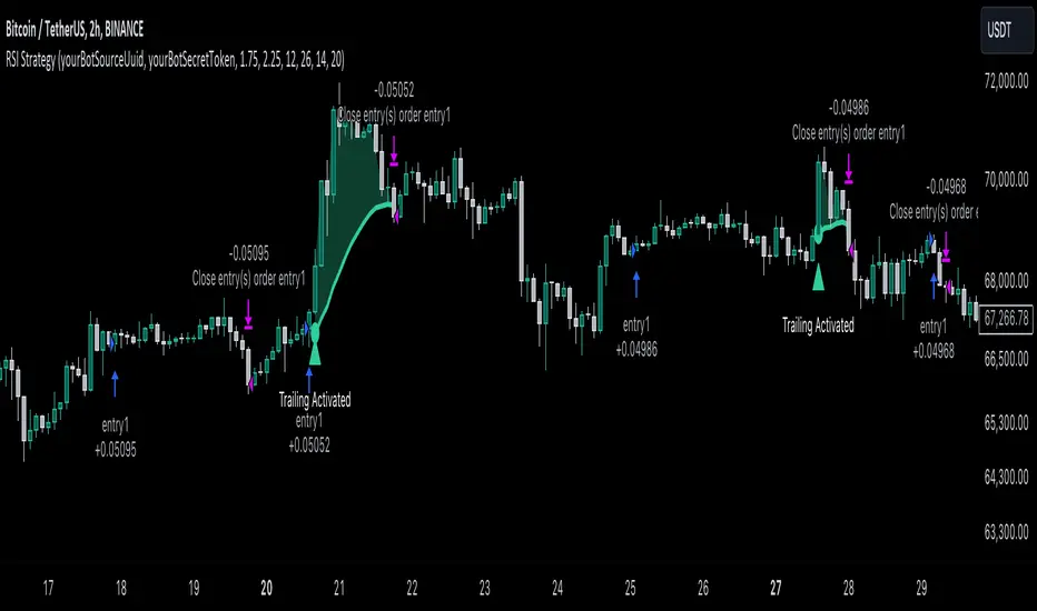
RSI Trend Following StrategyOverview
The RSI Trend Following Strategy utilizes Relative Strength Index (RSI) to enter the trade for the potential trend continuation. It uses Stochastic indicator to check is the price is not in overbought territory and the MACD to measure the current price momentum. Moreover, it uses the 200-period EMA to filter the counter trend trades with the higher probability. The strategy opens only long trades.
Unique Features
Dynamic stop-loss system: Instead of fixed stop-loss level strategy utilizes average true range (ATR) multiplied by user given number subtracted from the position entry price as a dynamic stop loss level.
Configurable Trading Periods: Users can tailor the strategy to specific market windows, adapting to different market conditions.
Two layers trade filtering system: Strategy utilizes MACD and Stochastic indicators measure the current momentum and overbought condition and use 200-period EMA to filter trades against major trend.
Trailing take profit level: After reaching the trailing profit activation level script activates the trailing of long trade using EMA. More information in methodology.
Wide opportunities for strategy optimization: Flexible strategy settings allows users to optimize the strategy entries and exits for chosen trading pair and time frame.
Methodology
The strategy opens long trade when the following price met the conditions:
RSI is above 50 level.
MACD line shall be above the signal line
Both lines of Stochastic shall be not higher than 80 (overbought territory)
Candle’s low shall be above the 200 period EMA
When long trade is executed, strategy set the stop-loss level at the price ATR multiplied by user-given value below the entry price. This level is recalculated on every next candle close, adjusting to the current market volatility.
At the same time strategy set up the trailing stop validation level. When the price crosses the level equals entry price plus ATR multiplied by user-given value script starts to trail the price with trailing EMA(by default = 20 period). If price closes below EMA long trade is closed. When the trailing starts, script prints the label “Trailing Activated”.
Strategy settings
In the inputs window user can setup the following strategy settings:
ATR Stop Loss (by default = 1.75)
ATR Trailing Profit Activation Level (by default = 2.25)
MACD Fast Length (by default = 12, period of averaging fast MACD line)
MACD Fast Length (by default = 26, period of averaging slow MACD line)
MACD Signal Smoothing (by default = 9, period of smoothing MACD signal line)
Oscillator MA Type (by default = EMA, available options: SMA, EMA)
Signal Line MA Type (by default = EMA, available options: SMA, EMA)
RSI Length (by default = 14, period for RSI calculation)
Trailing EMA Length (by default = 20, period for EMA, which shall be broken close the trade after trailing profit activation)
Justification of Methodology
This trading strategy is designed to leverage a combination of technical indicators—Relative Strength Index (RSI), Moving Average Convergence Divergence (MACD), Stochastic Oscillator, and the 200-period Exponential Moving Average (EMA)—to determine optimal entry points for long trades. Additionally, the strategy uses the Average True Range (ATR) for dynamic risk management to adapt to varying market conditions. Let's look in details for which purpose each indicator is used for and why it is used in this combination.
Relative Strength Index (RSI) is a momentum indicator used in technical analysis to measure the speed and change of price movements in a financial market. It helps traders identify whether an asset is potentially overbought (overvalued) or oversold (undervalued), which can indicate a potential reversal or continuation of the current trend.
How RSI Works? RSI tracks the strength of recent price changes. It compares the average gains and losses over a specific period (usually 14 periods) to assess the momentum of an asset. Average gain is the average of all positive price changes over the chosen period. It reflects how much the price has typically increased during upward movements. Average loss is the average of all negative price changes over the same period. It reflects how much the price has typically decreased during downward movements.
RSI calculates these average gains and losses and compares them to create a value between 0 and 100. If the RSI value is above 70, the asset is generally considered overbought, meaning it might be due for a price correction or reversal downward. Conversely, if the RSI value is below 30, the asset is considered oversold, suggesting it could be poised for an upward reversal or recovery. RSI is a useful tool for traders to determine market conditions and make informed decisions about entering or exiting trades based on the perceived strength or weakness of an asset's price movements.
This strategy uses RSI as a short-term trend approximation. If RSI crosses over 50 it means that there is a high probability of short-term trend change from downtrend to uptrend. Therefore RSI above 50 is our first trend filter to look for a long position.
The MACD (Moving Average Convergence Divergence) is a popular momentum and trend-following indicator used in technical analysis. It helps traders identify changes in the strength, direction, momentum, and duration of a trend in an asset's price.
The MACD consists of three components:
MACD Line: This is the difference between a short-term Exponential Moving Average (EMA) and a long-term EMA, typically calculated as: MACD Line = 12 period EMA − 26 period EMA
Signal Line: This is a 9-period EMA of the MACD Line, which helps to identify buy or sell signals. When the MACD Line crosses above the Signal Line, it can be a bullish signal (suggesting a buy); when it crosses below, it can be a bearish signal (suggesting a sell).
Histogram: The histogram shows the difference between the MACD Line and the Signal Line, visually representing the momentum of the trend. Positive histogram values indicate increasing bullish momentum, while negative values indicate increasing bearish momentum.
This strategy uses MACD as a second short-term trend filter. When MACD line crossed over the signal line there is a high probability that uptrend has been started. Therefore MACD line above signal line is our additional short-term trend filter. In conjunction with RSI it decreases probability of following false trend change signals.
The Stochastic Indicator is a momentum oscillator that compares a security's closing price to its price range over a specific period. It's used to identify overbought and oversold conditions. The indicator ranges from 0 to 100, with readings above 80 indicating overbought conditions and readings below 20 indicating oversold conditions.
It consists of two lines:
%K: The main line, calculated using the formula (CurrentClose−LowestLow)/(HighestHigh−LowestLow)×100 . Highest and lowest price taken for 14 periods.
%D: A smoothed moving average of %K, often used as a signal line.
This strategy uses stochastic to define the overbought conditions. The logic here is the following: we want to avoid long trades in the overbought territory, because when indicator reaches it there is a high probability that the potential move is gonna be restricted.
The 200-period EMA is a widely recognized indicator for identifying the long-term trend direction. The strategy only trades in the direction of this primary trend to increase the probability of successful trades. For instance, when the price is above the 200 EMA, only long trades are considered, aligning with the overarching trend direction.
Therefore, strategy uses combination of RSI and MACD to increase the probability that price now is in short-term uptrend, Stochastic helps to avoid the trades in the overbought (>80) territory. To increase the probability of opening long trades in the direction of a main trend and avoid local bounces we use 200 period EMA.
ATR is used to adjust the strategy risk management to the current market volatility. If volatility is low, we don’t need the large stop loss to understand the there is a high probability that we made a mistake opening the trade. User can setup the settings ATR Stop Loss and ATR Trailing Profit Activation Level to realize his own risk to reward preferences, but the unique feature of a strategy is that after reaching trailing profit activation level strategy is trying to follow the trend until it is likely to be finished instead of using fixed risk management settings. It allows sometimes to be involved in the large movements.
Backtest Results
Operating window: Date range of backtests is 2023.01.01 - 2024.08.01. It is chosen to let the strategy to close all opened positions.
Commission and Slippage: Includes a standard Binance commission of 0.1% and accounts for possible slippage over 5 ticks.
Initial capital: 10000 USDT
Percent of capital used in every trade: 30%
Maximum Single Position Loss: -3.94%
Maximum Single Profit: +15.78%
Net Profit: +1359.21 USDT (+13.59%)
Total Trades: 111 (36.04% win rate)
Profit Factor: 1.413
Maximum Accumulated Loss: 625.02 USDT (-5.85%)
Average Profit per Trade: 12.25 USDT (+0.40%)
Average Trade Duration: 40 hours
These results are obtained with realistic parameters representing trading conditions observed at major exchanges such as Binance and with realistic trading portfolio usage parameters.
How to Use
Add the script to favorites for easy access.
Apply to the desired timeframe and chart (optimal performance observed on 2h BTC/USDT).
Configure settings using the dropdown choice list in the built-in menu.
Set up alerts to automate strategy positions through web hook with the text: {{strategy.order.alert_message}}
Disclaimer:
Educational and informational tool reflecting Skyrex commitment to informed trading. Past performance does not guarantee future results. Test strategies in a simulated environment before live implementation
MACD with 1D Stochastic Confirmation Reversal StrategyOverview
The MACD with 1D Stochastic Confirmation Reversal Strategy utilizes MACD indicator in conjunction with 1 day timeframe Stochastic indicators to obtain the high probability short-term trend reversal signals. The main idea is to wait until MACD line crosses up it’s signal line, at the same time Stochastic indicator on 1D time frame shall show the uptrend (will be discussed in methodology) and not to be in the oversold territory. Strategy works on time frames from 30 min to 4 hours and opens only long trades.
Unique Features
Dynamic stop-loss system: Instead of fixed stop-loss level strategy utilizes average true range (ATR) multiplied by user given number subtracted from the position entry price as a dynamic stop loss level.
Configurable Trading Periods: Users can tailor the strategy to specific market windows, adapting to different market conditions.
Higher time frame confirmation: Strategy utilizes 1D Stochastic to establish the major trend and confirm the local reversals with the higher probability.
Trailing take profit level: After reaching the trailing profit activation level scrip activate the trailing of long trade using EMA. More information in methodology.
Methodology
The strategy opens long trade when the following price met the conditions:
MACD line of MACD indicator shall cross over the signal line of MACD indicator.
1D time frame Stochastic’s K line shall be above the D line.
1D time frame Stochastic’s K line value shall be below 80 (not overbought)
When long trade is executed, strategy set the stop-loss level at the price ATR multiplied by user-given value below the entry price. This level is recalculated on every next candle close, adjusting to the current market volatility.
At the same time strategy set up the trailing stop validation level. When the price crosses the level equals entry price plus ATR multiplied by user-given value script starts to trail the price with EMA. If price closes below EMA long trade is closed. When the trailing starts, script prints the label “Trailing Activated”.
Strategy settings
In the inputs window user can setup the following strategy settings:
ATR Stop Loss (by default = 3.25, value multiplied by ATR to be subtracted from position entry price to setup stop loss)
ATR Trailing Profit Activation Level (by default = 4.25, value multiplied by ATR to be added to position entry price to setup trailing profit activation level)
Trailing EMA Length (by default = 20, period for EMA, when price reached trailing profit activation level EMA will stop out of position if price closes below it)
User can choose the optimal parameters during backtesting on certain price chart, in our example we use default settings.
Justification of Methodology
This strategy leverages 2 time frames analysis to have the high probability reversal setups on lower time frame in the direction of the 1D time frame trend. That’s why it’s recommended to use this strategy on 30 min – 4 hours time frames.
To have an approximation of 1D time frame trend strategy utilizes classical Stochastic indicator. The Stochastic Indicator is a momentum oscillator that compares a security's closing price to its price range over a specific period. It's used to identify overbought and oversold conditions. The indicator ranges from 0 to 100, with readings above 80 indicating overbought conditions and readings below 20 indicating oversold conditions.
It consists of two lines:
%K: The main line, calculated using the formula (CurrentClose−LowestLow)/(HighestHigh−LowestLow)×100 . Highest and lowest price taken for 14 periods.
%D: A smoothed moving average of %K, often used as a signal line.
Strategy logic assumes that on 1D time frame it’s uptrend in %K line is above the %D line. Moreover, we can consider long trade only in %K line is below 80. It means that in overbought state the long trade will not be opened due to higher probability of pullback or even major trend reversal. If these conditions are met we are going to our working (lower) time frame.
On the chosen time frame, we remind you that for correct work of this strategy you shall use 30min – 4h time frames, MACD line shall cross over it’s signal line. The MACD (Moving Average Convergence Divergence) is a popular momentum and trend-following indicator used in technical analysis. It helps traders identify changes in the strength, direction, momentum, and duration of a trend in a stock's price.
The MACD consists of three components:
MACD Line: This is the difference between a short-term Exponential Moving Average (EMA) and a long-term EMA, typically calculated as: MACD Line=12-period EMA−26-period
Signal Line: This is a 9-period EMA of the MACD Line, which helps to identify buy or sell signals. When the MACD Line crosses above the Signal Line, it can be a bullish signal (suggesting a buy); when it crosses below, it can be a bearish signal (suggesting a sell).
Histogram: The histogram shows the difference between the MACD Line and the Signal Line, visually representing the momentum of the trend. Positive histogram values indicate increasing bullish momentum, while negative values indicate increasing bearish momentum.
In our script we are interested in only MACD and signal lines. When MACD line crosses signal line there is a high chance that short-term trend reversed to the upside. We use this strategy on 45 min time frame.
ATR is used to adjust the strategy risk management to the current market volatility. If volatility is low, we don’t need the large stop loss to understand the there is a high probability that we made a mistake opening the trade. User can setup the settings ATR Stop Loss and ATR Trailing Profit Activation Level to realize his own risk to reward preferences, but the unique feature of a strategy is that after reaching trailing profit activation level strategy is trying to follow the trend until it is likely to be finished instead of using fixed risk management settings. It allows sometimes to be involved in the large movements.
Backtest Results
Operating window: Date range of backtests is 2023.01.01 - 2024.08.01. It is chosen to let the strategy to close all opened positions.
Commission and Slippage: Includes a standard Binance commission of 0.1% and accounts for possible slippage over 5 ticks.
Initial capital: 10000 USDT
Percent of capital used in every trade: 30%
Maximum Single Position Loss: -4.79%
Maximum Single Profit: +20.14%
Net Profit: +2361.33 USDT (+44.72%)
Total Trades: 123 (44.72% win rate)
Profit Factor: 1.623
Maximum Accumulated Loss: 695.80 USDT (-5.48%)
Average Profit per Trade: 19.20 USDT (+0.59%)
Average Trade Duration: 30 hours
These results are obtained with realistic parameters representing trading conditions observed at major exchanges such as Binance and with realistic trading portfolio usage parameters.
How to Use
Add the script to favorites for easy access.
Apply to the desired timeframe between 30 min and 4 hours and chart (optimal performance observed on 45 min BTC/USDT).
Configure settings using the dropdown choice list in the built-in menu.
Set up alerts to automate strategy positions through web hook with the text: {{strategy.order.alert_message}}
Disclaimer:
Educational and informational tool reflecting Skyrex commitment to informed trading. Past performance does not guarantee future results. Test strategies in a simulated environment before live implementation

AlgoBuilder [Mean-Reversion] | FractalystWhat's the strategy's purpose and functionality?
This strategy is designed for both traders and investors looking to rely and trade based on historical and backtested data using automation.
The main goal is to build profitable mean-reversion strategies that outperform the underlying asset in terms of returns while minimizing drawdown.
For example, as for a benchmark, if the S&P 500 (SPX) has achieved an estimated 10% annual return with a maximum drawdown of -57% over the past 20 years, using this strategy with different entry and exit techniques, users can potentially seek ways to achieve a higher Compound Annual Growth Rate (CAGR) while maintaining a lower maximum drawdown.
Although the strategy can be applied to all markets and timeframes, it is most effective on stocks, indices, future markets, cryptocurrencies, and commodities and JPY currency pairs given their trending behaviors.
In trending market conditions, the strategy employs a combination of moving averages and diverse entry models to identify and capitalize on upward market movements. It integrates market structure-based moving averages and bands mechanisms across different timeframes and provides exit techniques, including percentage-based and risk-reward (RR) based take profit levels.
Additionally, the strategy has also a feature that includes a built-in probability function for traders who want to implement probabilities right into their trading strategies.
Performance summary, weekly, and monthly tables enable quick visualization of performance metrics like net profit, maximum drawdown, profit factor, average trade, average risk-reward ratio (RR), and more.
This aids optimization to meet specific goals and risk tolerance levels effectively.
-----
How does the strategy perform for both investors and traders?
The strategy has two main modes, tailored for different market participants: Traders and Investors.
Trading:
1. Trading:
- Designed for traders looking to capitalize on bullish trending markets.
- Utilizes a percentage risk per trade to manage risk and optimize returns.
- Suitable for active trading with a focus on mean-reversion and risk per trade approach.
◓: Mode | %: Risk percentage per trade
3. Investing:
- Geared towards investors who aim to capitalize on bullish trending markets without using leverage while mitigating the asset's maximum drawdown.
- Utilizes pre-define percentage of the equity to buy, hold, and manage the asset.
- Focuses on long-term growth and capital appreciation by fully investing in the asset during bullish conditions.
- ◓: Mode | %: Risk not applied (In investing mode, the strategy uses 10% of equity to buy the asset)
-----
What's is FRMA? How does the triple bands work? What are the underlying calculations?
Middle Band (FRMA):
The middle band is the core of the FRMA system. It represents the Fractalyst Moving Average, calculated by identifying the most recent external swing highs and lows in the market structure.
By determining these external swing pivot points, which act as significant highs and lows within the market range, the FRMA provides a unique moving average that adapts to market structure changes.
Upper Band:
The upper band shows the average price of the most recent external swing highs.
External swing highs are identified as the highest points between pivot points in the market structure.
This band helps traders identify potential overbought conditions when prices approach or exceed this upper band.
Lower Band:
The lower band shows the average price of the most recent external swing lows.
External swing lows are identified as the lowest points between pivot points in the market structure.
The script utilizes this band to identify potential oversold conditions, triggering entry signals as prices approach or drop below the lower band.
Adjustments Based on User Inputs:
Users can adjust how the upper and lower bands are calculated based on their preferences:
Upper/Lower: This method calculates the average bands using the prices of external swing highs and lows identified in the market.
Percentage Deviation from FRMA: Alternatively, users can opt to calculate the bands based on a percentage deviation from the middle FRMA. This approach provides flexibility to adjust the width of the bands relative to market conditions and volatility.
-----
What's the purpose of using moving averages in this strategy? What are the underlying calculations?
Using moving averages is a widely-used technique to trade with the trend.
The main purpose of using moving averages in this strategy is to filter out bearish price action and to only take trades when the price is trading ABOVE specified moving averages.
The script uses different types of moving averages with user-adjustable timeframes and periods/lengths, allowing traders to try out different variations to maximize strategy performance and minimize drawdowns.
By applying these calculations, the strategy effectively identifies bullish trends and avoids market conditions that are not conducive to profitable trades.
The MA filter allows traders to choose whether they want a specific moving average above or below another one as their entry condition.
This comparison filter can be turned on (>) or off.
For example, you can set the filter so that MA#1 > MA#2, meaning the first moving average must be above the second one before the script looks for entry conditions. This adds an extra layer of trend confirmation, ensuring that trades are only taken in more favorable market conditions.
⍺: MA Period | Σ: MA Timeframe
-----
What entry modes are used in this strategy? What are the underlying calculations?
The strategy by default uses two different techniques for the entry criteria with user-adjustable left and right bars: Breakout and Fractal.
1. Breakout Entries :
- The strategy looks for pivot high points with a default period of 3.
- It stores the most recent high level in a variable.
- When the price crosses above this most recent level, the strategy checks if all conditions are met and the bar is closed before taking the buy entry.
◧: Pivot high left bars period | ◨: Pivot high right bars period
2. Fractal Entries :
- The strategy looks for pivot low points with a default period of 3.
- When a pivot low is detected, the strategy checks if all conditions are met and the bar is closed before taking the buy entry.
◧: Pivot low left bars period | ◨: Pivot low right bars period
2. Hunt Entries :
- The strategy identifies a candle that wicks through the lower FRMA band.
- It waits for the next candle to close above the low of the wick candle.
- When this condition is met and the bar is closed, the strategy takes the buy entry.
By utilizing these entry modes, the strategy aims to capitalize on bullish price movements while ensuring that the necessary conditions are met to validate the entry points.
-----
What type of stop-loss identification method are used in this strategy? What are the underlying calculations?
Initial Stop-Loss:
1. ATR Based:
The Average True Range (ATR) is a method used in technical analysis to measure volatility. It is not used to indicate the direction of price but to measure volatility, especially volatility caused by price gaps or limit moves.
Calculation:
- To calculate the ATR, the True Range (TR) first needs to be identified. The TR takes into account the most current period high/low range as well as the previous period close.
The True Range is the largest of the following:
- Current Period High minus Current Period Low
- Absolute Value of Current Period High minus Previous Period Close
- Absolute Value of Current Period Low minus Previous Period Close
- The ATR is then calculated as the moving average of the TR over a specified period. (The default period is 14).
Example - ATR (14) * 2
⍺: ATR period | Σ: ATR Multiplier
2. ADR Based:
The Average Day Range (ADR) is an indicator that measures the volatility of an asset by showing the average movement of the price between the high and the low over the last several days.
Calculation:
- To calculate the ADR for a particular day:
- Calculate the average of the high prices over a specified number of days.
- Calculate the average of the low prices over the same number of days.
- Find the difference between these average values.
- The default period for calculating the ADR is 14 days. A shorter period may introduce more noise, while a longer period may be slower to react to new market movements.
Example - ADR (20) * 2
⍺: ADR period | Σ: ADR Multiplier
3. PL Based:
This method places the stop-loss at the low of the previous candle.
If the current entry is based on the hunt entry strategy, the stop-loss will be placed at the low of the candle that wicks through the lower FRMA band.
Example:
If the previous candle's low is 100, then the stop-loss will be set at 100.
This method ensures the stop-loss is placed just below the most recent significant low, providing a logical and immediate level for risk management.
Application in Strategy (ATR/ADR):
- The strategy calculates the current bar's ADR/ATR with a user-defined period.
- It then multiplies the ADR/ATR by a user-defined multiplier to determine the initial stop-loss level.
By using these methods, the strategy dynamically adjusts the initial stop-loss based on market volatility, helping to protect against adverse price movements while allowing for enough room for trades to develop.
Each market behaves differently across various timeframes, and it is essential to test different parameters and optimizations to find out which trailing stop-loss method gives you the desired results and performance.
-----
What type of break-even and take profit identification methods are used in this strategy? What are the underlying calculations?
For Break-Even:
Percentage (%) Based:
Moves the initial stop-loss to the entry price when the price reaches a certain percentage above the entry.
Calculation:
Break-even level = Entry Price * (1 + Percentage / 100)
Example:
If the entry price is $100 and the break-even percentage is 5%, the break-even level is $100 * 1.05 = $105.
Risk-to-Reward (RR) Based:
Moves the initial stop-loss to the entry price when the price reaches a certain RR ratio.
Calculation:
Break-even level = Entry Price + (Initial Risk * RR Ratio)
Example:
If the entry price is $100, the initial risk is $10, and the RR ratio is 2, the break-even level is $100 + ($10 * 2) = $120.
FRMA Based:
Moves the stop-loss to break-even when the price hits the FRMA level at which the entry was taken.
Calculation:
Break-even level = FRMA level at the entry
Example:
If the FRMA level at entry is $102, the break-even level is set to $102 when the price reaches $102.
For TP1 (Take Profit 1):
- You can choose to set a take profit level at which your position gets fully closed or 50% if the TP2 boolean is enabled.
- Similar to break-even, you can select either a percentage (%) or risk-to-reward (RR) based take profit level, allowing you to set your TP1 level as a percentage amount above the entry price or based on RR.
For TP2 (Take Profit 2):
- You can choose to set a take profit level at which your position gets fully closed.
- As with break-even and TP1, you can select either a percentage (%) or risk-to-reward (RR) based take profit level, allowing you to set your TP2 level as a percentage amount above the entry price or based on RR.
When Both Percentage (%) Based and RR Based Take Profit Levels Are Off:
The script will adjust the take profit level to the higher FRMA band set within user inputs.
Calculation:
Take profit level = Higher FRMA band length/timeframe specified by the user.
This ensures that when neither percentage-based nor risk-to-reward-based take profit methods are enabled, the strategy defaults to using the higher FRMA band as the take profit level, providing a consistent and structured approach to profit-taking.
For TP1 and TP2, it's specifying the price levels at which the position is partially or fully closed based on the chosen method (percentage or RR) above the entry price.
These calculations are crucial for managing risk and optimizing profitability in the strategy.
⍺: BE/TP type (%/RR) | Σ: how many RR/% above the current price
-----
What's the ADR filter? What does it do? What are the underlying calculations?
The Average Day Range (ADR) measures the volatility of an asset by showing the average movement of the price between the high and the low over the last several days.
The period of the ADR filter used in this strategy is tied to the same period you've used for your initial stop-loss.
Users can define the minimum ADR they want to be met before the script looks for entry conditions.
ADR Bias Filter:
- Compares the current bar ADR with the ADR (Defined by user):
- If the current ADR is higher, it indicates that volatility has increased compared to ADR (DbU).(⬆)
- If the current ADR is lower, it indicates that volatility has decreased compared to ADR (DbU).(⬇)
Calculations:
1. Calculate ADR:
- Average the high prices over the specified period.
- Average the low prices over the same period.
- Find the difference between these average values in %.
2. Current ADR vs. ADR (DbU):
- Calculate the ADR for the current bar.
- Calculate the ADR (DbU).
- Compare the two values to determine if volatility has increased or decreased.
By using the ADR filter, the strategy ensures that trades are only taken in favorable market conditions where volatility meets the user's defined threshold, thus optimizing entry conditions and potentially improving the overall performance of the strategy.
>: Minimum required ADR for entry | %: Current ADR comparison to ADR of 14 days ago.
-----
What's the probability filter? What are the underlying calculations?
The probability filter is designed to enhance trade entries by using buyside liquidity and probability analysis to filter out unfavorable conditions.
This filter helps in identifying optimal entry points where the likelihood of a profitable trade is higher.
Calculations:
1. Understanding Swing highs and Swing Lows
Swing High: A Swing High is formed when there is a high with 2 lower highs to the left and right.
Swing Low: A Swing Low is formed when there is a low with 2 higher lows to the left and right.
2. Understanding the purpose and the underlying calculations behind Buyside, Sellside and Equilibrium levels.
3. Understanding probability calculations
1. Upon the formation of a new range, the script waits for the price to reach and tap into equilibrium or the 50% level. Status: "⏸" - Inactive
2. Once equilibrium is tapped into, the equilibrium status becomes activated and it waits for either liquidity side to be hit. Status: "▶" - Active
3. If the buyside liquidity is hit, the script adds to the count of successful buyside liquidity occurrences. Similarly, if the sellside is tapped, it records successful sellside liquidity occurrences.
5. Finally, the number of successful occurrences for each side is divided by the overall count individually to calculate the range probabilities.
Note: The calculations are performed independently for each directional range. A range is considered bearish if the previous breakout was through a sellside liquidity. Conversely, a range is considered bullish if the most recent breakout was through a buyside liquidity.
Example - BSL > 55%
-----
What's the range length Filter? What are the underlying calculations?
The range length filter identifies the price distance between buyside and sellside liquidity levels in percentage terms. When enabled, the script only looks for entries when the minimum range length is met. This helps ensure that trades are taken in markets with sufficient price movement.
Calculations:
Range Length (%) = ( ( Buyside Level − Sellside Level ) / Current Price ) ×100
Range Bias Identification:
Bullish Bias: The current range price has broken above the previous external swing high.
Bearish Bias: The current range price has broken below the previous external swing low.
Example - Range length filter is enabled | Range must be above 1%
>: Minimum required range length for entry | %: Current range length percentage in a (Bullish/Bearish) range
-----
What's the day filter Filter, what does it do?
The day filter allows users to customize the session time and choose the specific days they want to include in the strategy session. This helps traders tailor their strategies to particular trading sessions or days of the week when they believe the market conditions are more favorable for their trading style.
Customize Session Time:
Users can define the start and end times for the trading session.
This allows the strategy to only consider trades within the specified time window, focusing on periods of higher market activity or preferred trading hours.
Select Days:
Users can select which days of the week to include in the strategy.
This feature is useful for excluding days with historically lower volatility or unfavorable trading conditions (e.g., Mondays or Fridays).
Benefits:
Focus on Optimal Trading Periods:
By customizing session times and days, traders can focus on periods when the market is more likely to present profitable opportunities.
Avoid Unfavorable Conditions:
Excluding specific days or times can help avoid trading during periods of low liquidity or high unpredictability, such as major news events or holidays.
Increased Flexibility: The filter provides increased flexibility, allowing traders to adapt the strategy to their specific needs and preferences.
Example - Day filter | Session Filter
θ: Session time | Exchange time-zone
-----
What tables are available in this script?
Table Type:
- Summary: Provides a general overview, displaying key performance parameters such as Net Profit, Profit Factor, Max Drawdown, Average Trade, Closed Trades and more.
Avg Trade: The sum of money gained or lost by the average trade generated by a strategy. Calculated by dividing the Net Profit by the overall number of closed trades. An important value since it must be large enough to cover the commission and slippage costs of trading the strategy and still bring a profit.
MaxDD: Displays the largest drawdown of losses, i.e., the maximum possible loss that the strategy could have incurred among all of the trades it has made. This value is calculated separately for every bar that the strategy spends with an open position.
Profit Factor: The amount of money a trading strategy made for every unit of money it lost (in the selected currency). This value is calculated by dividing gross profits by gross losses.
Avg RR: This is calculated by dividing the average winning trade by the average losing trade. This field is not a very meaningful value by itself because it does not take into account the ratio of the number of winning vs losing trades, and strategies can have different approaches to profitability. A strategy may trade at every possibility in order to capture many small profits, yet have an average losing trade greater than the average winning trade. The higher this value is, the better, but it should be considered together with the percentage of winning trades and the net profit.
Winrate: The percentage of winning trades generated by a strategy. Calculated by dividing the number of winning trades by the total number of closed trades generated by a strategy. Percent profitable is not a very reliable measure by itself. A strategy could have many small winning trades, making the percent profitable high with a small average winning trade, or a few big winning trades accounting for a low percent profitable and a big average winning trade. Most mean-reversion successful strategies have a percent profitability of 40-80% but are profitable due to risk management control.
BE Trades: Number of break-even trades, excluding commission/slippage.
Losing Trades: The total number of losing trades generated by the strategy.
Winning Trades: The total number of winning trades generated by the strategy.
Total Trades: Total number of taken traders visible your charts.
Net Profit: The overall profit or loss (in the selected currency) achieved by the trading strategy in the test period. The value is the sum of all values from the Profit column (on the List of Trades tab), taking into account the sign.
- Monthly: Displays performance data on a month-by-month basis, allowing users to analyze performance trends over each month.
- Weekly: Displays performance data on a week-by-week basis, helping users to understand weekly performance variations.
- OFF: Hides the performance table.
Profit Color:
- Allows users to set the color for representing profit in the performance table, helping to quickly distinguish profitable periods.
Loss Color:
- Allows users to set the color for representing loss in the performance table, helping to quickly identify loss-making periods.
These customizable tables provide traders with flexible and detailed performance analysis, aiding in better strategy evaluation and optimization.
-----
User-input styles and customizations:
To facilitate studying historical data, all conditions and rules can be applied to your charts. By plotting background colors on your charts, you'll be able to identify what worked and what didn't in certain market conditions.
Please note that all background colors in the style are disabled by default to enhance visualization.
-----
How to Use This Algobuilder to Create a Profitable Edge and System:
Choose Your Strategy mode:
- Decide whether you are creating an investing strategy or a trading strategy.
Select a Market:
- Choose a one-sided market such as stocks, indices, or cryptocurrencies.
Historical Data:
- Ensure the historical data covers at least 10 years of price action for robust backtesting.
Timeframe Selection:
- Choose the timeframe you are comfortable trading with. It is strongly recommended to use a timeframe above 15 minutes to minimize the impact of commissions/slippage on your profits.
Set Commission and Slippage:
- Properly set the commission and slippage in the strategy properties according to your broker or prop firm specifications.
Parameter Optimization:
- Use trial and error to test different parameters until you find the performance results you are looking for in the summary table or, preferably, through deep backtesting using the strategy tester.
Trade Count:
- Ensure the number of trades is 100 or more; the higher, the better for statistical significance.
Positive Average Trade:
- Make sure the average trade value is above zero.
(An important value since it must be large enough to cover the commission and slippage costs of trading the strategy and still bring a profit.)
Performance Metrics:
- Look for a high profit factor, and net profit with minimum drawdown.
- Ideally, aim for a drawdown under 20-30%, depending on your risk tolerance.
Refinement and Optimization:
- Try out different markets and timeframes.
- Continue working on refining your edge using the available filters and components to further optimize your strategy.
Automation:
- Once you’re confident in your strategy, you can use the automation section to connect the algorithm to your broker or prop firm.
- Trade a fully automated and backtested trading strategy, allowing for hands-free execution and management.
-----
What makes this strategy original?
1. Incorporating direct integration of probabilities into the strategy.
2. Utilizing built-in market structure-based moving averages across various timeframes.
4. Offering both investing and trading strategies, facilitating optimization from different perspectives.
5. Automation for efficient execution.
6. Providing a summary table for instant access to key parameters of the strategy.
-----
How to use automation?
For Traders:
1. Ensure the strategy parameters are properly set based on your optimized parameters.
2. Enter your PineConnector License ID in the designated field.
3. Specify the desired risk level.
4. Provide the Metatrader symbol.
5. Check for chart updates to ensure the automation table appears on the top right corner, displaying your License ID, risk, and symbol.
6. Set up an alert with the strategy selected as Condition and the Message as {{strategy.order.alert_message}}.
7. Activate the Webhook URL in the Notifications section, setting it as the official PineConnector webhook address.
8. Double-check all settings on PineConnector to ensure the connection is successful.
9. Create the alert for entry/exit automation.
For Investors:
1. Ensure the strategy parameters are properly set based on your optimized parameters.
2. Choose "Investing" in the user-input settings.
3. Create an alert with a specified name.
4. Customize the notifications tab to receive alerts via email.
5. Buying/selling alerts will be triggered instantly upon entry or exit order execution.
-----
Terms and Conditions | Disclaimer
Our charting tools are provided for informational and educational purposes only and should not be construed as financial, investment, or trading advice. They are not intended to forecast market movements or offer specific recommendations. Users should understand that past performance does not guarantee future results and should not base financial decisions solely on historical data.
Built-in components, features, and functionalities of our charting tools are the intellectual property of @Fractalyst Unauthorized use, reproduction, or distribution of these proprietary elements is prohibited.
By continuing to use our charting tools, the user acknowledges and accepts the Terms and Conditions outlined in this legal disclaimer and agrees to respect our intellectual property rights and comply with all applicable laws and regulations.
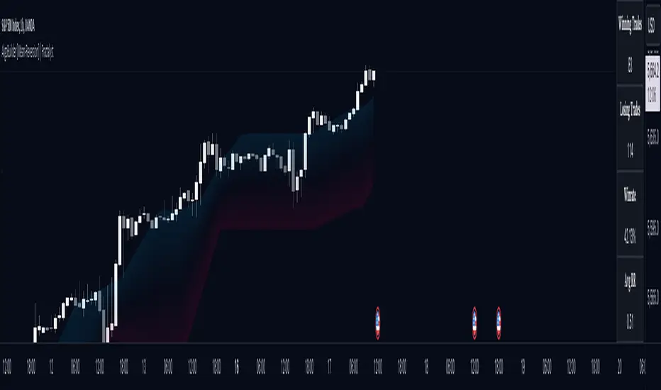
Ultimate Trading StrategyDescription:
In this TradingView Pine Script publication, we introduce a powerful tool designed to enhance your trading strategies by combining the Exponential Moving Average (EMA) and the Relative Strength Index (RSI). This strategy is specifically tailored for the EGLD/USDT.P pair on Binance, using a 5-minute interval to capture timely trading opportunities in a volatile market.
Key Features:
Combining EMA and RSI for Robust Signals
This script combines the EMA, which helps identify the overall trend direction, with the RSI, which measures the speed and change of price movements to identify overbought and oversold conditions.
The combination ensures that you get high-probability signals by leveraging both trend-following and momentum-based indicators.
Multiple Timeframe Analysis
Analyze the EMA and RSI across different timeframes to gain a comprehensive view of market conditions and make more informed trading decisions.
Reversing and Extending Signals
Reverse signals generated by indicators to adapt to various market conditions.
Extend signals by specifying conditions such as "RSI cross AND EMA cross WITHIN 2 bars" to capture more nuanced trading opportunities.
Backtesting and Risk Management
Evaluate the performance of your strategies by feeding the results into a backtesting engine.
The strategy risks a maximum of 10% of the account on a single trade to maintain sustainable risk levels.
Available Indicators:
EMA (Exponential Moving Average)
Helps identify the overall trend direction.
Signals:
Long Entry: When the price closes above the EMA.
Short Entry: When the price closes below the EMA.
RSI (Relative Strength Index)
Measures the speed and change of price movements.
Signals:
Long Entry: When RSI is below the oversold level (30).
Short Entry: When RSI is above the overbought level (70).
How It Works:
Long Entry: A buy signal is generated when the price closes above the EMA and the RSI is below the oversold level (30). This indicates that the price is in an upward trend and temporarily oversold, presenting a potential buying opportunity.
Short Entry: A sell signal is generated when the price closes below the EMA and the RSI is above the overbought level (70). This indicates that the price is in a downward trend and temporarily overbought, presenting a potential selling opportunity.
Close Long Position: The script closes long positions when the conditions for a short entry are met.
Close Short Position: The script closes short positions when the conditions for a long entry are met.
Parameters:
EMA Length: 20 (default)
RSI Length: 14 (default)
RSI Overbought Level: 70 (default)
RSI Oversold Level: 30 (default)
Initial Capital: 10,000 USDT (default) – Realistic starting capital for an average trader.
Commission: 0.1% (default) – Reflects typical trading commissions.
Slippage: 0.5 ticks (default) – Accounts for market conditions and potential price slippage during order execution.
Backtesting:
Trading Range: – Ensure that the dataset used covers a significant period to generate a sufficient number of trades.
Dataset Limitation: Due to TradingView Premium's limitation of backtesting only 20,000 candles, it may not be possible to generate more than 100 trades. This limitation affects the statistical relevance of the backtesting results, but the strategy has been tested to provide meaningful insights within these constraints.
Use Case:
This strategy combines the EMA and RSI to identify potential trading opportunities by detecting trend direction and overbought/oversold conditions. It is particularly effective in volatile markets where quick trend reversals are common.
How to Use:
Set the parameters according to your preference or use the default values.
Run the script on the EGLD/USDT.P pair with a 5-minute interval.
Monitor the signals and adjust your trades accordingly.

Strategy - Plus / Connectable [Azullian]Discover the advanced capabilities of Strategy Plus, an essential component of the connectable indicator system designed for fast-paced strategy testing, visualization, and building within TradingView. This enhanced version of our foundational connectable strategy indicator seamlessly integrates with all connectable indicators . By utilizing the TradingView input source as a signal connector , it facilitates the linking of indicators to form a cohesive strategy. Each connectable indicator within the system sends signal weight to the next node, culminating in a comprehensive strategy that incorporates advanced customization options, sophisticated signal interpretation, and elaborate backtest labeling. Strategy Plus stands out by offering improved position management and extensive alert messaging capabilities, ensuring effective strategy refinement and backend integration.
█ DISTINCTIVE FEATURES
The Connectable Strategy Plus enhances risk mitigation within the connectable system through its advanced features and capabilities:
• Refined Signal Input Management: Tailor and precisely connect up to two signal filters with enhanced input flexibility, gain control, and strategic direction settings.
• Strategic Position Investment Control: Optimize positioning with versatile investment bases, custom investment percentages, and direction-specific investments for effective risk management.
• Advanced Exit Stop Loss Configuration: Implement custom stop loss tactics with diverse base modes and trailing options for tailored risk management.
• Strategic Exit Take Profit Settings: Apply precision-driven take profit strategies with various calculation modes and dynamic trailing functionality.
• Calibrated Entry Position Allocation: Optimize investment distribution for entry positions, including DCA and BRO trades, for strategic market response.
• Refined Order Setting Customization: Ensure exchange compliance with adjustable order settings, enhancing backtest accuracy and strategy reliability.
• Comprehensive Condition Settings: Define precise conditions for strategy execution, including date range filtering and order/loss limitations.
• Intuitive Visualization: Enhance strategy clarity with customizable visual elements and trade visualization features.
• Advanced Alert Configurations: Stay informed with comprehensive and customizable alerts for effective backend integration.
• Backend Integration With JSON Format: Leverage elaborate and structured data in JSON format for advanced analytics, enhancing decision-making and strategy optimization outside TradingView.
Let's review the separate parts of this indicator.
█ STRATEGY INPUTS
We've provided 2 inputs for connecting a signal filter or indicators or chains (1→, 2→) which are all set to 'Close' by default.
An input has several controls:
• Enable disable: Toggle the entire input on or off
• Input: Connect indicators or signal filter here, choose indicators with a compatible : Signal connector.
• G - Gain: Increase or reduce the strength of the incoming signal by a factor.
• SM - Signal Mode: Choose a trading direction compatible with the settings in your signal filter
• XM - Exit Mode: Determine when to allow to exit your open trade
○ Always: Doesn't take the restrictions into account, this ignores all the settings chosen in ML or MP
○ Restricted: Use both ML and MP conditions
○ Loss: Use the ML condition only, for example: Position will be exited and the exit signal will be allowed only when the loss exceeds the ML parameter
○ Profit: Use the MP condition only for example: Exits will only be allowed when the profit of the position exceeds the condition of the MP parameter
█ POSITION INVESTMENT
Determine the percentage of your trading budget you would like to use in each position based on the strategy's profit or loss.
• LINVB - Loss Investment Base: Choose which base to use to determine the investment percentage when the strategy is in a loss.
○ Equity: Use the equity as the base for percentage calculation.
○ Initial capital: Use the initial capital as the base for percentage calculation.
• LINV% - Loss Investment Percentage: Set a percentage of the chosen investment base as the investment for a new position.
○ For example, when 10% in loss, and a initial capital of $100, and the investment base is set to equity with a percentage of 50%, your investment will be 50% of $90, $45.
• PINVB - Profit Investment Base: Choose which base to use to determine the investment percentage when the strategy is in profit.
○ Equity: Use the equity as the base for percentage calculation.
○ Initial capital: Use the initial capital as the base for percentage calculation.
• PINV% - Profit Investment Percentage: Set a percentage of the chosen investment base as the investment for a new position.
○ For example, when 10% in profit, and an initial capital of $100, and the investment base is set to equity with a percentage of 100%, your investment will be 100% of $110, $110.
• XINVB - Custom Profit Investment Base: Choose which base to use to determine the investment percentage when the strategy is above a custom profit threshold (XT).
○ Equity: Use the equity as the base for percentage calculation.
○ Initial capital: Use the initial capital as the base for percentage calculation.
• XINV% - Custom Profit Investment Percentage: Set a percentage of the chosen investment base as the investment for a new position.
○ For example, when 100% in profit, exceeding the XT threshold of 50%, and an initial capital of $100, and the investment base is set to equity with a percentage of 50%, your investment will be 50% of $200, $100.
• XT% - Custom Profit Threshold: Determine how much profit triggers these custom profit investment settings.
• ELIB% - Entry Long Investment Base: Following previous settings, you can further restrict the investment according to the long trading direction.
○ For instance, if the previous calculation resulted in $45 to be used as an investment, and you've set the ELIB% to 50%, your long position will use 50% of $45, which is $22.5.
• ESIB% - Entry Short Investment Base: Following previous settings, you can further restrict the investment according to the short trading direction.
○ For example, if the previous calculation resulted in $45 to be used as an investment, and you've set the ESIB% to 50%, your short position will use 50% of $45, which is $22.5.
• RISK% - Risk Percentage:
○ Determine how much of the calculated position investment is at risk when the stop-loss is hit.
- For example, 1% of $45 represents a maximum loss of $0.45.
○ Risk percentage works together with the stop loss and the max leverage.
• MXLVG - Maximum Leverage:
○ Investigate the trading rules for your trading pair and use the maximum allowed amount of leverage.
○ To determine the number of contracts to be bought or sold, considering the stop loss and the specified risk percentage, the maximum leverage available will constrain the amount of leverage utilized to ensure that the maximum risk threshold is not exceeded. For instance, suppose the stop loss is set at 1%, and the risk percentage is defined as 10%. Initially, the calculated leverage to be used would be 10. However, if there is a maximum leverage cap set at 5, it would constrain the calculated leverage of 10 to adhere to the maximum limit of 5.
█ EXIT STOP LOSS
Determine the Stop Loss price based on your selected configuration.
As the stop loss is an integral part of the ordered contracts calculation used in conjunction with the Risk and Max leverage, you'll always need to provide a stop loss price.
• SLLB - Stop Loss Long Base: Choose a stop loss mode for calculating stop loss prices in long positions.
○ Risk: Determines the price using the Risk parameter (RISK%) and maximum leverage (MXLVG). In this case, SLLB% will not have any impact.
○ Price Entry + Offset: Calculates the stop loss price based on a offset percentage (SLLB%) from the entry price of the position.
○ Source: Computes the stop loss price based on an external indicator defined in SLLSRC.
- If this results in an invalid price, the calculation will revert to using the price entry + offset.
○ Source + Offset: Determines the stop loss price based on a positive or negative offset percentage (SLLB%) from an external indicator defined in SLLSRC.
- If this results in an invalid price, the calculation will fall back to using the price entry + offset.
• SLLB% - Stop Loss Long Base Percentage: Define an offset percentage that will be applied in the price entry + offset and source + offset stop loss modes.
• SLLSRC - Stop Loss Long Source: Connect an external indicator as the source for stop loss (only those providing price values eg: bollinger bands, moving averages...).
• SLLT - Stop Loss Long Trailing:
○ Fixed: The initial stop loss will be kept and no trailing stop loss will be applied.
○ Trail Stop: Takes into account all settings defined in SLLB and SLLB% and recalculates them with each candle.
- If a better stop loss is computed, it replaces the existing stop loss. In this mode SLLT% will be disregarded.
○ Trail Stop till BE: Similar to trailing stop mode, but it stops trailing when the stop loss reaches the break-even point.
○ Trail Stop from BE: Similar to trailing stop mode, but it starts trailing when the stop loss reaches the break-even point.
○ Trail Price: Computes the trailing stop loss price based on an offset percentage (SLLT%) from the closing price of the current candle.
- If a better stop loss price is calculated, it will be set as the new stop loss price.
○ Trail Price till BE: Similar to the Trail Price mode, but it stops trailing when the stop loss reaches the break-even point.
○ Trail Price from BE: Similar to Trail Price mode, but it starts trailing when the stop loss reaches the break-even point.
○ Trail Incr: Adapts the trailing stop loss price based on the offset percentage (SLLT%).
- Each price change in favor of your position will incrementally adapt the trailing stop loss with SLLT%.
○ Trail Incr till BE: Similar to the Trail Incr mode, but it stops trailing when the stop loss reaches the break-even point.
• SLLT% - Stop Loss Long Trailing Percentage: This percentage serves as an offset or increment depending on your chosen trailing mode.
• SLSB - Stop Loss Short Base: Functions similarly to SLLB but for short positions.
• SLSB% - Stop Loss Short Base Percentage: Functions similarly to SLLB% but for short positions.
• SLSSRC - Stop Loss Short Source: Functions similarly to SLLSRC but for short positions.
• SLST - Stop Loss Short Trailing: Functions similarly to SLLT but for short positions.
• SLST% - Stop Loss Short Trailing Percentage: Functions similarly to SLLT% but for short positions.
█ EXIT TAKE PROFIT
Determine the Take Profit price based on your selected configuration.
• TPLB - Take Profit Long Base: Choose a take profit mode for calculating take profit prices in long positions.
○ Reward: Determines the take profit price using the Risk parameter (RISK%) and the calculated Stop Loss price and the set reward percentage (TPLB%).
- For example: Risk 1%, Calculated Stop loss price: $90, Entry price: $100, Reward (TPLB%): 2%, will result in a take profit price on $120.
○ Price Entry + Offset: Calculates the take profit price based on a offset percentage (TPLB%) from the entry price of the position.
- For example: Entry price: $100, Offset (TPLB%): 2%, will result in a take profit price on $102.
○ Source: Computes the take profit price based on an external input from another indicator defined in TPLSRC.
- If this results in an invalid price, the calculation will revert to using the price entry + offset.
○ Source + Offset: Determines the take profit price based on a positive or negative offset percentage (TPLB%) from an external indicator inpuy defined in TPLSRC.
- If this results in an invalid price, the calculation will fall back to using the price entry + offset.
• TPLB% - Take Profit Long Base Percentage: Define an offset percentage that will be applied in the price entry + offset and source + offset take profit modes.
• TPLSRC - Take Profit Long Source: Choose to connect an external indicator as the source for take profit (of course only those which provide price values eg: bollinger bands, moving averages... but not oscillators).
• TPLT - Take Profit Long Trailing:
○ Fixed: The initial take profit will be kept and no trailing take profit will be applied.
○ Trail Profit: Takes into account all settings defined in TPLB and TPLB% and recalculates them with each candle.
- If an applicable take profit is computed, it replaces the existing take profit. In this mode TPLT% will be disregarded.
○ Trail Profit till BE: Similar to trailing profit mode, but it stops trailing when the take profit reaches the break-even point.
○ Trail Profit from BE: Similar to trailing profit mode, but it starts trailing when the take profit reaches the break-even point.
○ Trail Price: Computes the trailing take profit price based on an offset percentage (TPLT%) from the closing price of the current candle.
- If an applicable take profit price is calculated, it will be set as the new take profit price.
○ Trail Price till BE: Similar to the Trail Price mode, but it stops trailing when the take profit reaches the break-even point.
○ Trail Price from BE: Similar to Trail Price mode, but it starts trailing when the take profit reaches the break-even point.
○ Trail Incr: Adapts the trailing take profit price based on the offset percentage (TPLT%). Each price change against your position will incrementally adapt the trailing take profit with TPLT%.
○ Trail Incr till BE: Similar to the Trail Incr mode, but it stops trailing when the take profit reaches the break-even point.
• TPLT% - Take Profit Long Trailing Percentage: This percentage serves as an offset or increment depending on your chosen trailing mode.
• TPSB - Take Profit Short Base: Functions similarly to TPLB but for short positions.
• TPSB% - Take Profit Short Base Percentage: Functions similarly to TPLB% but for short positions.
• TPSSRC - Take Profit Short Source: Functions similarly to TPLSRC but for short positions.
• TPST - Take Profit Short Trailing: Functions similarly to TPLT but for short positions.
• TPST% - Take Profit Short Trailing Percentage: Functions similarly to TPLT% but for short positions.
█ ENTRY INVESTMENT DISTRIBUTION
Based on your position investment calculation you can distribute the position investment accross the initial opening trade of the position (SIG%) or the follow up Dollar Cost Averaging (DCA%) or Break Out (BRO%) trades.
For example: SIG%: 10%, DCA%: 45%, BRO%: 45% and the calculated Position Investment is $100, then the initial trade will receive $10, DCA will receive $45, and BRO will receive $45 to work with. Disable BRO and or DCA by setting them to 0%. Keep in mind that the sum of SIG, BRO and DCA may not exceed 100%.
• SIG% - Initial order investment percentage based on the signal: The percentage of the position investment distributed over normal trades.
• DCA% - Dollar Cost Averaging investment percentage: The percentage of the position investment distributed to DCA trades.
• BRO% - Break Out investment percentage: The percentage of the position investment distributed to BRO trades.
█ ENTRY DCA
DCA (Dollar-Cost Averaging) is a risk mitigation strategy where the allocated DCA% budget from the Entry Investment Distribution is distributed among x levels (DCA#) based on calculated prices (DPLM) and order sizes (DOSM), when prices move against your position.
• DCA# - Maximum DCA levels: Set the maximum number of DCA levels.
• DPLM - DCA Price Level Mode: Choose a price level mode that determines at which prices the additional purchases are distributed:
○ Linear: Entry prices are evenly spaced at regular intervals.
○ QuadIn: Entry prices are front-loaded, with more at the beginning and fewer later.
○ QuadOut: Entry prices are back-loaded, with fewer at the beginning and more later.
○ QuadInOut: Entry prices start front-loaded, then become back-loaded.
○ CubicIn: Similar to QuadIn but with a smoother front-loaded distribution.
○ CubicOut: Similar to QuadOut but with a smoother back-loaded distribution.
○ ExpoIn: Entry prices are exponentially increasing, starting small and growing.
○ ExpoOut: Entry prices are exponentially decreasing, starting large and reducing.
○ ExpoInOut: Entry prices start exponentially increasing, then decrease exponentially.
• DOSM - DCA Order Size Mode: Choose a DCA budget distribution mode for order sizes:
○ Linear: Order sizes are evenly spaced at regular intervals.
○ QuadIn: Order sizes are front-loaded, with larger orders at the beginning and smaller ones later.
○ QuadOut: Order sizes are back-loaded, with smaller orders at the beginning and larger ones later.
○ QuadInOut: Order sizes start front-loaded and transition to back-loaded.
○ CubicIn: Similar to QuadIn but with a smoother front-loaded distribution of order sizes.
○ CubicOut: Similar to QuadOut but with a smoother back-loaded distribution of order sizes.
○ ExpoIn: Order sizes exponentially increase, starting small and growing.
○ ExpoOut: Order sizes exponentially decrease, starting large and reducing.
○ ExpoInOut: Order sizes start exponentially increasing, then decrease exponentially.
For a visual representation of the price or order size distribution modes, refer to online easing curves.
█ ENTRY BRO
BRO (Break Out) is a risk mitigation strategy where the allocated BRO% budget from the Entry Investment Distribution is distributed among x levels (BRO#) based on calculated prices (BPLM) and order sizes (BOSM), when prices move in favor of your position.
• BRO# - Maximum BRO levels: Set the maximum number of BRO levels.
• BPLM - BRO Price Level Mode: Choose a price level mode that determines at which prices the additional purchases are distributed:
○ Distribution easing modes work similar as the DCA easing modes.
• BOSM - BRO Order Size Mode: Choose a BRO budget distribution mode for order sizes:
○ Distribution easing modes work similar as the DCA easing modes.
█ ORDER SETTINGS
Fine-tune accuracy to match your exchange's trading constraints, enhancing backtest precision with these settings, default settings are least restrictive for crypto trading pairs.
• MINP - Mininmum Position Notional Value: Exchange-defined minimum notional value for positions:
○ Calculated based on your exchange's rules and is the minimum total value your position must hold to meet their requirements It is calculated by multiplying Quantity with price and leverage.
○ It helps ensure your trades align with your exchange's standards.
• MAXP - Maximum Position Notional Value: Exchange-defined maximum notional value for positions:
○ Similar to MINP, this value is calculated based on your exchange's rules and represents the maximum total value allowed for your position.
• MINQ - Mininmum Order Quantity: Least permissible order quantity based on exchange rules:
○ This is the smallest quantity of an asset that your exchange allows you to trade in a single order.
• MAXQ - Maximum Order Quantity: Highest permissible order quantity according to exchange rules:
○ Opposite of MINQ, this is the largest quantity of an asset you can trade in a single order as defined by your exchange.
• DECP - Decimals in Order Price: Allowed decimal places in order prices as per exchange specifications:
○ This value specifies the number of decimal places you can use when specifying the price of an order.
• DECQ - Decimals in Order Quantity: Permitted decimal places in order quantities according to exchange specifications:
○ Similar to DECP, this value indicates the number of decimal places you can use when specifying the quantity of an asset in an order.
█ STRATEGY CONDITIONS
Specify when the strategy is permitted to execute trades.
• DATE: Enable the Date Range filter to restrict entries to a specific date range.
○ START: Set a start date and hour to commence trading.
○ END: Set an end date and hour to conclude trading within the defined range.
• IDO - Maximum Intraday Orders: Limit the number of orders the strategy can place within a single trading day. Upon reaching this limit, the strategy temporarily halts further entries for the day.
• DL% - Maximum Intraday Loss%: Set a threshold for the maximum allowable intraday loss as a percentage of equity. When exceeded, the strategy temporarily suspends trading for the day.
• CLD - Maximum Consecutive Loss Days: Define the maximum number of consecutive days the strategy can incur losses. Upon reaching this limit, the strategy halts trading and avoids new entries.
• DD% - Maximum Drawdown: Specify the maximum permissible drawdown as a percentage of equity. If this limit is met, the strategy halts trading and refrains from placing additional entries.
• TP% - Total Profit %: Establish a target for the total profit percentage the strategy aims to achieve. Once this target is attained, the strategy halts trading and refrains from initiating new entries.
• TL% - Total Loss %: Define a limit for the total loss percentage relative to the initial capital. If this limit is exceeded, the strategy discontinues trading and refrains from placing further entries.
■ VISUALS
• LINE: Activate a colored dashed diagonal line to visually connect the entry and exit points of positions.
• SLTP: Enable visualization of stop loss, take profit, and break-even levels.
• PNL: Enable Break-Even and Close Lines along with a colored area in between to visualize profit and loss.
• ☼: Brightness % : Adjust the opacity of the plotted trading visuals.
• P - Profit Color : Choose the color for profit-related elements.
• L - Loss Color: Choose the color for loss-related elements.
• B - Breakeven Color : Select the color for break-even points.
• EL - Long Color: Specify the color for long positions.
• ES - Short Color: Specify the color for short positions.
• TRADE LABELING: For better analysis we've labeled all entries and exits conform with the type of order your strategy has executed, some examples:
○ EL-SIG0-124: Enter Long - Signal 0 - Position 124
○ EL-BRO1-130: Enter Long - BRO1 - Position 130
○ EL-BRO2-130: Enter Long - BRO2 - Position 130
○ ES-DCA1-140: Enter Short - DCA1 - Position 140
○ XS-DCA2-140: Exit Short - DCA2 - Position 140
○ XL-TP-150: Exit Long - Take Profit - Position 150
○ XS-TP-154: Exit Short - Take Profit - Position 154
○ XL-SL-160: Exit Long - Stop Loss - Position 160
○ XS-SL-164: Exit Short - Stop Loss - Position 164
○ XS-CND-165: Exit Short - Strategy Condition - Max intraday loss - Position 165
■ ALERT SETTINGS
For developers and those who wish to integrate TradingView alerts into their backend systems, we offer comprehensive labeling options.
• ALID: A unique identifier you've assigned to your alert.
• NAME: A structured name you've given to this strategy.
• LAYOUT: The layout key of the strategy, allowing direct chart linking from your backend.
• SYMBOL: The symbol on which the strategy operates.
○ ONCE: You can choose to include this information only in the first message to reduce message size and repetition in follow-up messages. (max. 4096 characters)
• TICK: The ticker for the strategy.
• CHART: The chart parameter containing the timeframe.period and timeframe.multiplier.
○ ONCE: You can choose to include this information only in the first message to reduce message size and repetition in follow-up messages. (max. 4096 characters)
• BAR: Includes bar information in the alert message.
• STRATEGY: Adds strategy inputs to the alert message.
○ ONCE: You can choose to include this information only in the first message to reduce message size and repetition in follow-up messages. (max. 4096 characters)
• PERFORMANCE: Incorporates strategy performance data into the alert message.
• SIGNAL: Appends received signal weights (EL, XL, ES, XS) to the alert message.
• ORDERS: Includes order details in the alert message.
• TAGS: Adds up to 6 tags and their corresponding values to the alert message.
○ ONCE: You can choose to include this information only in the first message to reduce message size and repetition in follow-up messages. (max. 4096 characters)
Of course we can't neglect letting you in on how this juicy JSON would look (without the // comments):
{
"id": 20726, // Message Id
"t": "2023-11-01T10:35:00Z", // Message Time
"al": { // Alert
"id": "639bfa9a-5f01-4031-8880-7ec01e972055", // Alert Id
"n": "TEST04", // Name
"l": "ABC123" // Layout
},
"sym": { // Symbol
"typ": "crypto", // Type
"r": "DOGEUSD.PM", // Root
"pre": "KRAKEN", // Prefix
"tc": "DOGEUSD.PM", // Ticker
"bc": "DOGE", // BaseCurrency
"c": "USD", // Currency
"d": "DOGEUSD Multi Collateral Perpetual Futures Contract", // Description
"mtc": 0.000001, // MinTick
"pv": 1, // PointValue
"ct": "PF_DOGEUSD" // CustomTicker
},
"ch": { // Chart
"pd": "1", // Period
"mul": 1 // Multiplier
},
"bar": { // Bar
"id": 20725, // Index
"t": "2023-11-01T10:33:00Z", // Time
"o": 0.066799, // Open
"h": 0.066799, // High
"l": 0.066799, // Low
"c": 0.066799, // Close
"v": 2924 // Vol
},
"strat": { // Strategy
"n": "Strategy - Plus / Connectable ", // Name
"sig": { // Signal
"c1e": true, // Connector1Enabled
"c1s": 500500.500501, // Connector1Source
"c1g": 1, // Connector1Gain
"c2e": false, // Connector2Enabled
"c2s": 0.067043, // Connector2Source
"c2g": 1, // Connector2Gain
"sm": "Swing (EL, ES)", // SignalMode
"xm": "Always", // ExitMode
"mlp": 0.01, // ExitModeMinPercLoss
"mpp": 0.01 // ExitModeMinPercProfit
},
"inv": { // Investment
"lb": "Equity", // LossBase
"lp": 50, // LossPerc
"pb": "Equity", // ProfitBase
"pp": 100, // ProfitPerc
"pcb": "Equity", // ProfitCustomBase
"pcp": 100, // ProfitCustomPerc
"pct": 10000, // ProfitCustomThreshold
"elp": 100, // LongPerc
"esp": 100, // ShortPerc
"rsk": 1, // MaxRisk
"lvg": 10 // MaxLeverage
},
"sl": { // StopLoss
"lb": "Price Entry + Offset", // LongBase
"lp": 0.2, // LongPerc
"lsrc": 0.067043, // LongSource
"lt": "Trail Stop", // LongTrailMode
"ltp": 0.2, // LongTrailPerc
"sb": "Price Entry + Offset", // ShortBase
"sp": 0.2, // ShortPerc
"ssrc": 0.067043, // ShortSource
"st": "Trail Stop", // ShortTrailMode
"stp": 0.2 // ShortTrailPerc
},
"tp": { // TakeProfit
"lb": "Price Entry + Offset", // LongBase
"lp": 1, // LongPerc
"lsrc": 0.067043, // LongSource
"lt": "Fixed", // LongTrailMode
"ltp": 1, // LongTrailPerc
"sb": "Price Entry + Offset", // ShortBase
"sp": 1, // ShortPerc
"ssrc": 0.067043, // ShortSource
"st": "Fixed", // ShortTrailMode
"stp": 1 // ShortTrailPerc
},
"dis": { // Distribution
"sigp": 10, // SignalPerc
"dcap": 0, // DCAPerc
"brop": 90 // BROPerc
},
"dca": { // DCA
"lvl": 3, // Levels
"pl": "linear", // ModePriceLevel
"os": "linear" // ModeOrderSize
},
"bro": { // BRO
"lvl": 3, // Levels
"pl": "expoIn", // ModePriceLevel
"os": "cubicOut" // ModeOrderSize
},
"ord": { // OrderSettings
"pmin": 5, // PNVMin
"pmax": 30000000, // PNVMax
"qmin": 0, // QtyMin
"qmax": 1000000000, // QtyMax
"dp": 6, // DecPrice
"dq": 6 // DecQty
},
"cnd": { // Conditions
"de": true, // DateRangeEnabled
"start": "2023-11-01T10:30:00Z", // StartTime
"end": "2024-12-31T23:30:00Z", // EndTime
"idoe": false, // MaxIntradayOrdersEnabled
"ido": 100, // MaxIntradayOrders
"dle": false, // MaxIntradayLossEnabled
"dl": 10, // MaxIntradayLossPerc
"clde": false, // MaxConsLossDaysEnabled
"cld": false, // MaxConsLossDays
"dde": false, // MaxDrawdownEnabled
"dd": 100, // MaxDrawdownPerc
"mpe": false, // MaxProfitEnabled
"mp": 200, // MaxProfitPerc
"mle": false, // MaxLossEnabled
"ml": -50 // MaxLossPerc
}
},
"perf": { // Performance
"ic": 1000, // InitialCapital
"eq": 1000, // Equity
"np": 0, // NetProfit
"op": 0, // OpenProfit
"ct": 0, // ClosedTrades
"ot": 0, // OpenTrades
"p": "FLAT", // MarketPosition
"ps": 0, // MarketPositionSize
"pp": "FLAT", // PreviousMarketPosition
"pps": 0 // PreviousMarketPositionSize
},
"sig": { // Signal
"el": 0, // EL
"xl": 0, // XL
"es": 6, // ES
"xs": 0 // XS
},
"ord": ,
"tag":
}
█ USAGE OF CONNECTABLE INDICATORS
■ Connectable chaining mechanism
Connectable indicators can be connected directly to the signal monitor, signal filter or strategy , or they can be daisy chained to each other while the last indicator in the chain connects to the signal monitor, signal filter or strategy. When using a signal filter you can chain the filter to the strategy input to make your chain complete.
• Direct chaining: Connect an indicator directly to the signal monitor, signal filter or strategy through the provided inputs (→).
• Daisy chaining: Connect indicators using the indicator input (→). The first in a daisy chain should have a flow (⌥) set to 'Indicator only'. Subsequent indicators use 'Both' to pass the previous weight. The final indicator connects to the signal monitor, signal filter, or strategy.
■ Set up this indicator with signals and a signal filter
The indicator provides visual cues based on signal conditions. However, its weight system is best utilized when paired with a connectable signal filter, monitor, or strategy .
Let's connect the Strategy - Plus to a connectable signal filter and connectable indicators :
1. Load all relevant indicators
• Load MA - Plus / Connectable
• Load Signal filter - Plus / Connectable
• Load Strategy - Plus / Connectable
2. Signal Filter Plus: Connect the MA - Plus to the Signal Filter
• Open the signal filter settings
• Choose one of the five input dropdowns (1→, 2→, 3→, 4→, 5→) and choose : MA - Plus / Connectable: Signal Connector
• Toggle the enable box before the connected input to enable the incoming signal
3. Signal Filter: Update the filter settings if needed
• The default filter mode for the trading direction is SWING, and is compatible with the default settings in the strategy and indicators.
4. Signal Filter: Update the weight threshold settings if needed
• All connectable indicators load by default with a score of 6 for each direction (EL, XL, ES, XS)
• By default, weight threshold is 'ABOVE' Threshold 1 (TH1) and Threshold 2 (TH2), both set at 5. This allows each occurrence to score, as the default score is 1 point above the threshold.
5. Strategy Plus: Connect one of the strategy plus inputs to the signal filters signal connector in the strategy settings
• Select a strategy input → and select the Signal filter - Plus: Signal connector
6. Strateg Plus: Enable filter compatible directions
• As the default setting of the filter is SWING, we should also set the SM (Strategy mode) to SWING.
7. Strateg Plus: You're ready to start optimizing
• Dive into all parameters and start optimizing your backtesting results.
█ BENEFITS
• Adaptable Modular Design: Arrange indicators in diverse structures via direct or daisy chaining, allowing tailored configurations to align with your analysis approach.
• Streamlined Backtesting: Simplify the iterative process of testing and adjusting combinations, facilitating a smoother exploration of potential setups.
• Intuitive Interface: Navigate TradingView with added ease. Integrate desired indicators, adjust settings, and establish alerts without delving into complex code.
• Signal Weight Precision: Leverage granular weight allocation among signals, offering a deeper layer of customization in strategy formulation.
• Advanced Signal Filtering: Define entry and exit conditions with more clarity, granting an added layer of strategy precision.
• Clear Visual Feedback: Distinct visual signals and cues enhance the readability of charts, promoting informed decision-making.
• Standardized Defaults: Indicators are equipped with universally recognized preset settings, ensuring consistency in initial setups across different types like momentum or volatility.
• Reliability: Our indicators are meticulously developed to prevent repainting. We strictly adhere to TradingView's coding conventions, ensuring our code is both performant and clean.
█ COMPATIBLE INDICATORS
Each indicator that incorporates our open-source 'azLibConnector' library and adheres to our conventions can be effortlessly integrated and used as detailed above.
For clarity and recognition within the TradingView platform, we append the suffix ' / Connectable' to every compatible indicator.
█ COMMON MISTAKES, CLARIFICATIONS AND TIPS
• Removing an indicator from a chain: Deleting a linked indicator and confirming the "remove study tree" alert will also remove all underlying indicators in the object tree. Before removing one, disconnect the adjacent indicators and move it to the object stack's bottom.
• Point systems: The azLibConnector provides 500 points for each direction (EL: Enter long, XL: Exit long, ES: Enter short, XS: Exit short) Remember this cap when devising a point structure.
• Flow misconfiguration: In daisy chains the first indicator should always have a flow (⌥) setting of 'indicator only' while other indicator should have a flow (⌥) setting of 'both'.
• Hide attributes: As connectable indicators send through quite some information you'll notice all the arguments are taking up some screenwidth and cause some visual clutter. You can disable arguments in Chart Settings / Status line.
• Layout and abbreviations: To maintain a consistent structure, we use abbreviations for each input. While this may initially seem complex, you'll quickly become familiar with them. Each abbreviation is also explained in the inline tooltips.
• Inputs: Connecting a connectable indicator directly to the strategy delivers the raw signal without a weight threshold, meaning every signal will trigger a trade.
• Layout and Abbreviations: Abbreviations streamline structure and input identification. Although they may seem complex initially, inline tooltips provide explanations, facilitating quick acclimatization.
• Total Trade Limit Error & Date-Time Filter: For deep backtesting, be mindful of the total trade limit. Utilize the date-time filter to narrow the test scope and avoid TradingView order limits.
• Calculation Timeout: Encounter a timeout? Adjust any parameter slightly to restart the calculation process.
• Message Character Limit: To stay within message character limits, consider turning off certain features or setting some to 'once'.
• Direct Indicator-to-Strategy Connection: When connecting an indicator directly to a strategy without thresholds, the strategy will default to long if weights are equally assigned.
• Pyramid Enabling with DCA and BRO: Activate pyramid orders, enabling you to optimize your strategy during Dollar Cost Averaging and Break Out trades.
• Recalculate & Fill Orders Properties: Adjusting these default settings in strategy properties tab may lead to unexpected behavior when backtesting. Approach with caution.
• Optimized for Crypto: Our indicators have been optimized and tested primarily on cryptocurrency markets. Results in other markets may vary.
• Inline Tooltips Documentation: Detailed documentation and guidance are available via inline tooltips for immediate assistance.
• Strategy Settings Margin: Set margin to 1 to be able to apply leverage.
• Styling Panel: Explore the styling panel to disable labels or any other visual cues to reduce clutter on busy charts, enhancing visual clarity and personalization.
• Applying Leverage on Spot Markets: Ensure that maximum leverage on spot markets is configured to 1.
• Unrealistic Order Sizes: Verify that the order book can accommodate your backtested order sizes.
█ A NOTE OF GRATITUDE
Through years of exploring TradingView and Pine Script, we've drawn immense inspiration from the community's knowledge and innovation. Thank you for being a constant source of motivation and insight.
█ RISK DISCLAIMER
Azullian's content, tools, scripts, articles, and educational offerings are presented purely for educational and informational uses. Please be aware that past performance should not be considered a predictor of future results.
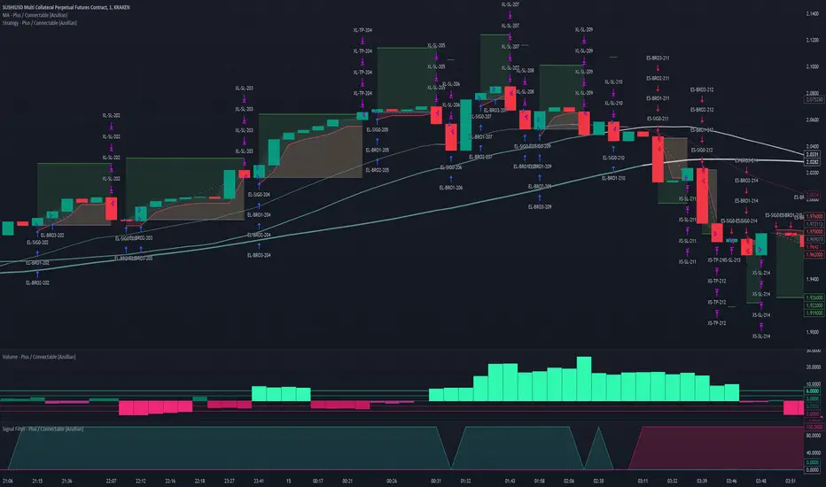
Crypto Market Strategy (CMS)/Introduction
The Crypto Market Strategy (CMS) is a composite strategy for the cryptocurrency market. It integrates multiple strategies (called signals) to ensure you are exploiting multiple patterns/anomalies in the market.
/Signals
The three distinct strategies, each providing signals based on specific market conditions are explained below:
1. Limit Range: This signal targets stable market periods, triggering signals based on micro breakouts in price. The market during this period is described as stable because of the short lookback period required for breakout, four bars is the default.
2. Trend Breakout: This signal seeks to capitalize on significant market movements following consolidation periods, it triggers when large price breakouts occur. The market during this period is described as volatile because of the long lookback period required for breakout, forty bars is the default.
3. Momentum: After breakouts, price uptrends may persist for a long time, typically weeks to months. This signal captures long term trends.
An upward blue arrow signifies a long entry signal, a downward red arrow indicates a short entry signal, while an upward/downward pink arrow indicates an exit signal. All signals will have a label indicating the triggering strategy and number of units (this can be disabled in the style settings).
/Construction
The strategy is constructed using minimal indicators, it is basically price action and moving averages.
/Settings
The settings are organised according to the signals;
1. Limit range
Entry - This is the size of breakout
+Exit - Closes the trade in profit
-Exit - Closes the trade to minimise loss
2. Trend breakout
Entry - This is the size of the breakout
Exit - Closes the trade to minimise loss
3. Momentum
Entry - This determines how quickly a signal is triggered
Lookback - This is the duration considered for the entry
/Results
The backtest results are based on a starting capital of $13,700 (convenient amount for retail traders) with 5% of equity for the position size and pyramiding of 3 consecutive positions because there are three signals. Commissions vary from broker to broker with some charging zero commissions, so commissions is set to an exorbitant $3 per order to ensure profitability in backtests is reproducible in live trading. Slippage of 3 ticks is used to ensure the results are representative of real world, market order, end-of-day trading. The backtest results are available to view at the bottom of this page.
Note:
Past performance in backtesting does not guarantee future results. Cryptocurrency markets are particularly volatile, and individual execution and market changes can significantly affect strategy performance. Price data may also vary across exchanges.
/Tickers
CMS has been backtested primarily on BTCUSD. It also performs well on ETHUSD.
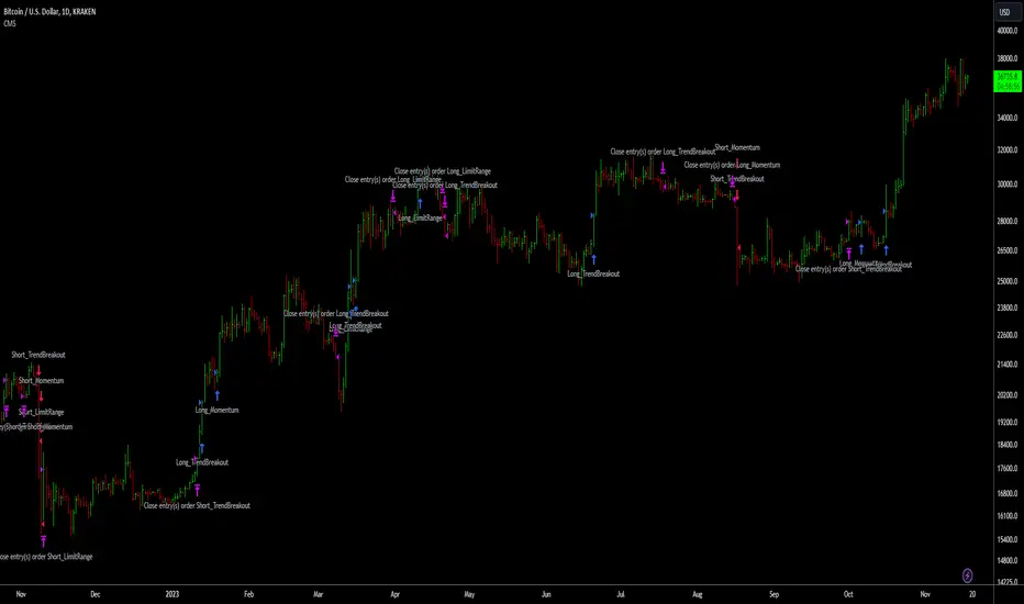
DZ Strategy ICTThe script presented is a trading strategy called "Breaker Block Strategy with Price Channel". This strategy uses multiple time frames (1 minute, 5 minutes, 15 minutes, 1 hour, and 4 hours) to detect support and resistance areas on the chart.
The strategy uses parameters such as length, deviations, multiplier, Fibonacci level, move lag and volume threshold for each time frame. These parameters are adjustable by the user.
The script then calculates support and resistance levels using the simple moving average (SMA) and standard deviation (STDEV) of closing prices for each time frame.
It also detects "Breaker Blocks" based on price movement from support and resistance levels, as well as trade volume. A Breaker Block occurs when there is a significant breakout of a support or resistance level with high volume.
Buy and sell signals are generated based on the presence of a Breaker Block and price movement from support and resistance levels. When a buy signal is generated, a buy order is placed, and when a sell signal is generated, a sell order is placed.
The script also plots price channels for each time frame, representing resistance and support levels.
Profit limit levels are set for each time range, indicating that the price levels assigned to positions should be closed with a profit. Stop-loss levels are also set to limit losses in the event of canceled price movements.
In summary, this trading strategy uses a combination of Breaker Block detection, support and resistance levels, price channels and profit limit levels to generate buy and sell signals and manage positions on different time ranges.
FVG Strategy - Fair Value GapThe Fair Value Gap Strategy (FVG) is a trading approach that relies on price action analysis and involves identifying market inefficiencies or imbalances.
The strategy offers a variety of customizable settings to match your preferences and includes an entry and exit strategy to guide you through trades.
The script operates in the following manner:
It begins by searching for fair-value-gaps and subsequently identifies a break in structure.
The next step involves waiting for the price to retrace within the previously established fair value gap.
Within this gap, there is a Fibonacci retracement that must be reached before placing a stop-order.
Example: GER40, 1min Chart
STOP LOSS & RISK MANAGEMENT
FVG : The stop loss will be set at the end of the fair value gap
Last Swing : The stop loss will be at the last swing high/low
ATR (Average True Range) : The stop loss will be placed one 'Average True Range' away from the entry
TAKE PROFIT
Pips/Points : The stop loss will be set at the chosen amount of pips/points.
RiskReward TP : This is a fixed take profit where you can set a specific risk-to-reward ratio for the trade. For example, you can set a 1:3 risk-to-reward ratio.
Trailing Stop : This is a flexible stop that moves with the market price, allowing you to capture more profit as the trade moves in your favor.
Both : This option combines both the RiskReward TP and Trailing Stop. If the price target is set at a 1:3 risk-to-reward ratio, the trailing stop will move with the price until either the stop or take profit is reached, and the position will be closed completely.
THE FVG SECTION
In the FVG section, you will have the ability to customize your settings based on your specific requirements.
Firstly, you will have the choice of two possible entry options:
Candle Close : This option triggers the order once the candle has completely closed and all the set requirements are met.
Stop Orders : This option triggers the order once all the set requirements are met, even if the candle is still active and has not yet closed.
On top, you can activate the "Pinbar-Trading", that will allow you to take a trade on a pinbar, even when the candle just dipped into the FVG and snapped back.
FAIR VALUE GAP TYPE
On volatile market, it may happen that a massive FVG is created. Thats why we have separated the FVG into 2 different variables.
FVG Type: Normal : This is all regular FVG that meet the requirement of you minimum size range. As example FVG must be minimum 5$ big.
FVG Type: Big : This are all big FVG that meet the minimum set size range. The difference to the "normal" type, the stop loss will be set at 50% of the Big-FVG.
FIBONACCI RETRACEMENT & MARKET STRUCTURE
To refine the FVG strategy, you have three options:
Fibonacci Retracement Value (%) : The FVG strategy employs a Fibonacci retracement, which allows you to trade in the direction of the market movement. To initiate the order, the price must reach a predetermined Fibonacci level and then rebound.
Formation-to-Retracement Countdown: : This option provides you with a specified number of candles to meet the necessary conditions. For example, if the order is not triggered within 20 candles, delete the FVG-Zone and skip the trade to avoid getting caught in a sideways ranging trend.
Structure Lookback : This feature filters out older FVG Zones. You can specify the number of candles that should mark the FVG Zones. Keep in mind that newer and fresher zones will automatically conceal older ones.
Strategy Myth-Busting #7 - MACDBB+SSL+VSF - [MYN]This is part of a new series we are calling "Strategy Myth-Busting" where we take open public manual trading strategies and automate them. The goal is to not only validate the authenticity of the claims but to provide an automated version for traders who wish to trade autonomously.
Our seventh one we are automating is the "Magic MACD Indicator: Crazy Accurate Scalping Trading Strategy ( 74% Win Rate )" strategy from "TradeIQ" who claims to have backtested this manually and achieved 427% profit with a 74% winrate over 100 trades in just a 4 months. I was unable to emulate these results consistently accommodating for slippage and commission but even so the results and especially the high win-rate and low markdown is pretty impressive and quite respectable.
This strategy uses a combination of 3 open-source public indicators:
AK MACD BB v 1.00 by Algokid
SSL Hybrid by Mihkel00
Volume Strength Finder by Saravanan_Ragavan
This is considered a trend following Strategy. AK MACD BB is being used as the primary short term trend direction indicator with an interesting approach of using Bollinger Bands to define an upper and lower range and upon the MACD going above the upper Bollinger Bands, it's indicative of an up trend, where as if the MACD is below the lower Bollinger Band, it's indicative of a down trend. To eliminate false signals, SSL Hyrbid is used as a trend confirmation filter, confirming and eliminating false signals from the MACD BB. It does this by validating the price action is above the the EMA and the SSL is positive that is a confirmation of an uptrend. When the price action is below the EMA and the SSL is negative, that is an confirmation of a downtrend. To avoid taking trades during ranged markets, VSF Buyer's Strength is used so the buyers/sellers strength and must be above 50% or the trade will not be inititiated.
Trading Rules
5 min candles but other lower time frames even below 5m work quite well too.
Best results can be found by tweaking these 2 input parameters:
Number Of bars to look back to ensure MACD isn't above/below Zero Line
Number Of bars back to look for SSL pullback
Long Entry when these conditions are true
AK MACD BB BB issues a new continuation long signal. A new green circle must appear on the indicator and these circles should not be touching across the zero level while they were previously red
SSL Hybrid price action closes above the EMA and the line is blue color and then creates a pullback . The pullback is confirmed when the color changes from blue to gray or from blue to red.
VSF Buyers strength above 50% at the time the MACD indicator issues a new long signal.
Short Entry when these conditions are true
AK MACD BB issues a new continuation short signal. A new red circle must appear on the indicator and these circles should not be touching across the zero level while they were previously green
SSL Hybrid price action closes below the EMA and the line is red color then it has to create a pullback . The pullback is confirmed when the color changes from red to gray or from red to blue.
VSF Sellers strength above 50% at the time the MACD indicator issues a new short signal.
Stop Loss at EMA Line with TP Target 1.5x the risk
If you know of or have a strategy you want to see myth-busted or just have an idea for one, please feel free to message me.
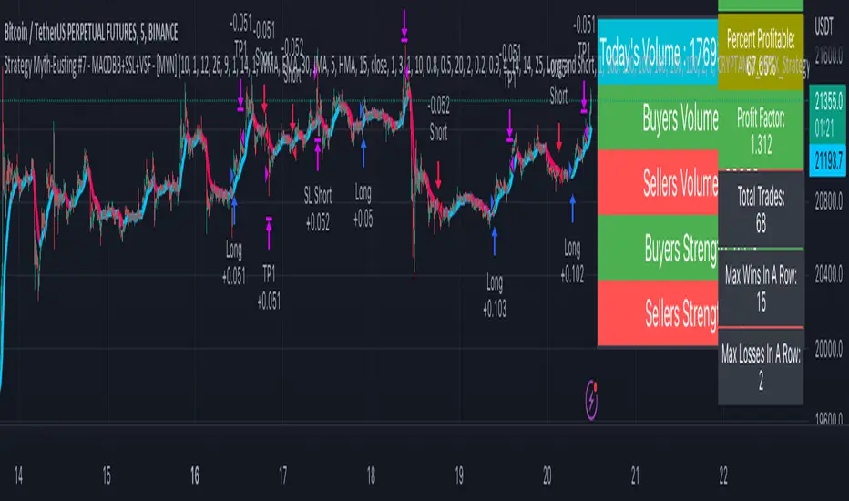
MACD + RSI + ADX Strategy (ChatGPT-powered) by TradeSmartThis is a trading strategy made by TradeSmart, using the recommendations given by ChatGPT . As an experiment, we asked ChatGPT on which indicators are the most popular for trading. We used all of the recommendations given, and added more. We ended up with a strategy that performs surprisingly well on many crypto and forex assets. See below for exact details on what logic was implemented and how you can change the parameters of the strategy.
The strategy is a Christmas special , this is how we would like to thank the support of our followers.
The strategy has performed well on Forex, tested on 43 1-hour pairs and turned a profit in 21 cases. Also it has been tested on 51 crypto pairs using the 1-hour timeframe, and turned a profit in 45 cases with a Profit Factor over 1.4 in the top-5 cases. Tests were conducted without commission or slippage, unlike the presented result which uses 0.01% commission and 5 tick slippage.
Some of the top performers were:
SNXUSDT
SOLUSDT
CAKEUSDT
LINKUSDT
EGLDUSDT
GBPJPY
TRYJPY
USDJPY
The strategy was implemented using the following logic:
Entry strategy:
Long entry:
Price should be above the Simple Moving Average (SMA)
There should be a cross up on the MACD (indicated by the color switch on the histogram, red to green)
RSI should be above the 50 level
Volume is above the selected volume-based Exponential Moving Average (EMA)
ADX should also agree to this position: below 50 and over 20, and above the Regularized Moving Average (REMA)
Short entry:
Price should be under the Simple Moving Average (SMA)
There should be a cross down on the MACD (indicated by the color switch on the histogram, red to green)
RSI should be below the 50 level
Volume is above the selected volume-based Exponential Moving Average (EMA)
ADX should also agree to this position: below 50 and over 20, and above the Regularized Moving Average (REMA)
Exit strategy:
Stop Loss will be placed based on ATR value (with 1.5 Risk)
Take profit level will be placed with a 2.5 Risk/Reward Ratio
Open positions will be closed early based on the Squeeze Momentum (Long: change to red, Short: change to green)
NOTE! : The position sizes used in the example is with 'Risk Percentage (current)', according which the position size will be determined such
that the potential loss is equal to % of the current available capital. This means that in most of the cases, the positions are calculated using leverage.
Parameters of every indicator used in the strategy can be tuned in the strategy settings as follows:
Plot settings:
Plot Signals: true by default, Show all Long and Short signals on the signal candle
Allow early TP/SL plots: false by default, Checking this option will result in the TP and SL lines to be plotted also on the signal candle rather than just the entry candle. Consider this only when manual trading, since backtest entries does not happen on the signal candle.
Entry Signal:
Fast Length: 12 by default
Slow Length: 26 by default
Source: hlcc4 by default
Signal Smoothing: 9 by default
Oscillator MA Type: EMA by default
Signal Line MA Type: EMA by default
Exit Strategy:
ATR Based Stop Loss: true by default
ATR Length (of the SL): 14 by default
ATR Smoothing (of the SL): EMA by default
Candle Low/High Based Stop Loss: false by default, recent lowest or highest point (depending on long/short position) will be used to calculate stop loss value. Set 'Base Risk Multiplier' to 1 if you would like to use the calculated value as is. Setting it to a different value will count as an additional multiplier. Please select only one active stop loss. Default value (if nothing or multiple stop losses are selected) is the 'ATR Based Stop Loss'.
Candle Lookback (of the SL): 10 by default
Base Risk Multiplier: 1.5 by default, the stop loss will be placed at this risk level (meaning in case of ATR SL that the ATR value will be multiplied by this factor and the SL will be placed that value away from the entry level)
Risk to Reward Ratio: 2.5 by default, the take profit level will be placed such as this Risk/Reward ratio is met
Force Exit based on Squeeze Momentum: true by default, a Long position will be closed when Squeeze Momentum turns red inside an open position and a Short position will be closed when Squeeze Momentum turns green inside an open position
BB Length: 20 by default
BB Mult Factor: 1.0 by default
KC Length: 20 by default
KC Mult Factor: 1.5 by default
Use True Range (KC): Yes by default
Base Setups:
Allow Long Entries: true by default
Allow Short Entries: true by default
Order Size: 1.5 by default
Order Type: Risk Percentage (current) by default, allows adjustment on how the position size is calculated: Cash: only the set cash ammount will be used for each trade Contract(s): the adjusted number of contracts will be used for each trade Capital Percentage: a % of the current available capital will be used for each trade Risk Percentage (current): position size will be determined such that the potential loss is equal to % of the current available capital Risk Percentage (initial): position size will be determined such that the potential loss is equal to % of the initial capital
Trend Filter:
Use long trend filter: true by default, only enter long if price is above Long MA
Show long trend filter: true by default, plot the selected MA on the chart
MA Type (Long): SMA by default
MA Length (Long): 100 by default
MA Source (Long): close by default
Use short trend filter: true by default, only enter long if price is under Short MA
Show short trend filter: false by default, plot the selected MA on the chart
MA Type (Short): SMA by default
MA Length (Short): 100 by default
MA Source (Short): close by default
Simple RSI Limiter:
Limit using Simple RSI: true by default, if set to 'Normal', only enter long when Simple RSI is lower then Long Boundary, and only enter short when Simple RSI is higher then Short Boundary. If set to 'Reverse', only enter long when Simple RSI is higher then Long Boundary, and only enter short when Simple RSI is lower then Short Boundary.
Simple RSI Limiter Type:
RSI Length: 14 by default
RSI Source: hl2 by default
Simple RSI Long Boundary: 50 by default
Simple RSI Short Boundary: 50 by default
ADX Limiter:
Use ADX Limiter: true by default, only enter into any position (long/short) if ADX value is higher than the Low Boundary and lower than the High Boundary.
ADX Length: 5 by default
DI Length: 5 by default
High Boundary: 50 by default
Low Boundary: 20 by default
Use MA based calculation: Yes by default, if 'Yes', only enter into position (long/short) if ADX value is higher than MA (ADX as source).
MA Type: REMA by default
MA Length: 5 by default
Volume Filter:
Only enter trades where volume is higher then the volume-based MA: true by default, a set type of MA will be calculated with the volume as source, and set length
MA Type: EMA by default
MA Length: 10 by default
Session Limiter:
Show session plots: false by default, show crypto market sessions on chart: Sidney (red), Tokyo (orange), London (yellow), New York (green)
Use session limiter: false by default, if enabled, trades will only happen in the ticked sessions below.
Sidney session: false by default, session between: 15:00 - 00:00 (EST)
Tokyo session: false by default, session between: 19:00 - 04:00 (EST)
London session: false by default, session between: 03:00 - 11:00 (EST)
New York session: false by default, session between: 08:00 - 17:00 (EST)
Date Range:
Limit Between Dates: false by default
Start Date: Jul 01 2021 00:00:00 by default
End Date: Dec 31 2022 00:00:00 by default
Trading Time:
Limit Trading Time: false by default, tick this together with the options below to enable limiting based on day and time
Valid Trading Days Global: 1234567 by default, if the Limit Trading Time is on, trades will only happen on days that are present in this field. If any of the not global Valid Trading Days is used, this field will be neglected. Values represent days: Sunday (1), Monday (2), ..., Friday (6), Saturday(7) To trade on all days use: 123457
(1) Valid Trading Days: false, 1234567 by default, values represent days: Sunday (1), Monday (2), ..., Friday (6), Saturday(7) The script will trade on days that are present in this field. Please make sure that this field and also (1) Valid Trading Hours Between is checked
(1) Valid Trading Hours Between: false, 0930-1600 by default, hours between which the trades can happen. The time is always in the exchange's timezone
Fine-tuning is highly recommended when using other asset/timeframe combinations.
LuxAlgo - Backtester (S&O)The S&O Backtester is an innovative strategy script that encompasses features + optimization methods from our Signals & Overlays™ toolkit and combines them into one easy-to-use script for backtesting the most detailed trading strategies possible.
Our Signals & Overlays™ toolkit is notorious for its signal optimization methods such as the 'Optimal Sensitivity' displayed in its dashboard which provides optimization backtesting of the Sensitivity parameter for the Confirmation & Contrarian Signals.
This strategy script allows even more detailed & precise backtests than anything available previously in the Signals & Overlays™ toolkit; including External Source inputs allowing users to use any indicator including our other paid toolkits for take profit & stop loss customization to develop strategies, along with 10+ pre-built filters directly Signals & Overlays™' features.
🔶 Features
Full Sensitivity optimization within the dashboard to find the Best Win rates or Best Profits.
Counter Trade Mode to reverse signals in undesirable market conditions (may introduce higher drawdowns)
Built-in filters for Confirmation Signals w/ Indicator Overlays from Signals & Overlays™.
Built-in Confirmation exit points are available within the settings & on by default.
External Source Input to filter signals or set custom Take Profits & Stop Losses.
Optimization Matrix dashboard option showing all possible permutations of Sensitivity.
Option to Maximize for Winrate or Best Profit.
🔶 Settings
Sensitivity signal optimizations for the Confirmation Signals algorithm
Buy & Sell conditions filters with Indicator Overlays & External Source
Take Profit exit signals option
External Source for Take Profit & Stop Loss
Sensitivity ranges
Backtest window default at 2,000 bars
External source
Dashboard locations
🔶 Usage
Backtests are not necessarily indicative of future results, although a trader may want to use a strategy script to have a deeper understanding of how their strategy responds to varying market conditions, or to use as a tool for identifying possible flaws in a strategy that could potentially be indicative of good or bad performance in the future.
A strategy script can also be useful in terms of it's ability to generate more complete & configurable alerts, giving users the option to integrate with external processes.
In the chart below we are using default settings and built-in optimization parameters to generate the highest win rate.
Results like the above will vary & finding a strategy with a high win rate does not necessarily mean it will persist into the future, however, some indications of a well-optimized strategy are:
A high number of closed trades (100+) with a consistently green equity curve
An equity curve that outperforms buy & hold
A low % max drawdown compared to the Net Profit %.
Profit factor around 1.5 or above
In the chart below we are using the Trend Catcher feature from Signals & Overlays™ as a filter for standard Confirmation Signals + exits on a higher timeframe.
By filtering bullish signals only when the Trend Catcher is bullish, as well as bearish signals for when the Trend Catcher is bearish, we have a highly profitable strategy created directly from our flagship features.
While the Signals & Overlays features being used as built-in filters can generate interesting backtests, the provided External Sources can allow for even more creativity when creating strategies. This feature allows you to use many indicators from TradingView as filters or to trigger take-profit/stop-loss events, even if they aren't from LuxAlgo.
The chart below shows the HyperWave Oscillator from our Oscillator Matrix™ being used for take-profit exit conditions, exiting a long position on a profit when crossing 80, and exiting a short position when crossing 20.
🔶 Counter Trade Mode
Our thesis has always firmly remained to use Confirmation Signals within Signals & Overlays™ as a supportive tool to find trends & use as extra confirmation within strategies.
We included the counter-trade mode as a logical way to use the Confirmation signals as direct entries for longs & shorts within more contrarian trading strategies. Many traders can relate to using a trend-following indicator and having the market not respect its conditions for entries.
This mode directly benefits a trader who is aware that market conditions are generally not-so-perfect trends all the time. Acknowledging this, allows the user to use this to their advantage by introducing countertrend following conditions as direct entries, which tend to perform very well in ranging markets.
The big downfall of using counter-trade mode is the potential for very large max-drawdowns during trending market conditions. We suggest for making a strategy to consider introducing stop-loss conditions that can efficiently minimize max-drawdowns during the process of backtesting your creations.
Sensitivity Optimization
Within the Signals & Overlays™ toolkit, we allow users to adjust the Confirmation Signals with a Sensitivity parameter.
We believe the Sensitivity paramter is the most realistic way to generate the most actionable Confirmation Signals that can navigate various market conditions, and the Confirmation Signals algorithm was designed specifically with this in mind.
This script takes this parameter and backtests it internally to generate the most profitable value to display on the dashboard located in the top right of the chart, as well as an optimization table if users enable it to visualize it's backtesting.
In the image below, we can see the optimization table showing permutations of settings within the user-selected Sensitivity range.
The suggested best setting is given at the current time for the backtesting window that's customizable within the indicator. Optimized settings for technical indicators are not indicative of future results and the best settings are highly likely / guaranteed to change over time.
Optimizing signal settings has become a popular activity amongst technical analysts, however, the real-time beneficial applications of optimizing settings are limited & best described as complicated (even with forward testing).
🔶 Strategy Properties (Important)
We strongly recommend all users to ensure they adjust the Properties within the script settings to be in line with their accounts & trading platforms of choice to ensure results from strategies built are realistic.
🔶 How to access
You can see the Author's Instructions below to learn how to get access on our website.

Miyagi BacktesterMiyagi: The attempt at mastering something for the best results.
Miyagi indicators combine multiple trigger conditions and place them in one toolbox for traders to easily use, produce alerts, backtest, reduce risk and increase profitability.
The Miyagi Backtester is a standalone backtester which is to be applied to the chart after the Miyagi indicator to be backtested.
The backtester can only backtest one script at a time, and is meant to backtest ONCE PER BAR CLOSE entries.
It is currently not possible to backtest ONCE PER BAR entries.
The backtester will allow users to all Miyagi Indicators using DCA strategies to show returns over a selectable time period.
The backtester allows leverage, and as such users should be aware of the Maximum Amount for Bot Usage and Leverage Required Calculations.
The DCA Selector switch will allow users to backtest with, or without DCA.
Static DCA is used within the backtester and allows users to see DCA Statistics on closed trades.
How to use the Miyagi Backtester
Step 1: Apply the Miyagi Indicator of Choice to backtest (4in1/10in1/Strend).
DATE AND TIME RANGE:
-Date and time range to backtest.
TRADE:
-Entry source to backtest. Please select the "Outbound Entry Signal Sender"
-Trade Direction to backtest. This can be helpful to backtest according to your strategy (long or short).
-Take Profit % to backtest. This is the percent take profit to backtest. Slippage can be accounted for on the "Properties" tab.
-Stoploss % to backtest. This is the percent stoploss to backtest.
DCA:
DCA Checkbox: Enable the DCA Checkbox to backtest with DCA. Disable it to backtest without DCA.
Leverage: Input the Leverage you will trade with.
Base Order Size (% Equity): This is the Base order (BO) size to backtest in % of equity.
Safety Order Size (% Equity): This is the Safety order (SO) size to backtest in % of equity.
Number of DCA Orders: This is the maximum amount of DCA orders to place, or total DCA orders.
Price Deviation (% from initial order): This is the percent at which the first safety is placed.
Safety Order Step Scale: This is the scale at which is applied to the deviation for the step calculation to determine next SO placement.
Safety Order Volume Scale: This is the scale at which is applied to the safety orders for the volume calculation to determine SO Volume.
Real world DCA Example:
The process is as follows.
Base Order: This is your initial order size, $100 used for Base Order
Safety Order: This is your first safety order size, which is placed at the deviation. $100 Safety Order, it is good to keep the same size as your BO for your scaling to be effective.
Price deviation: This is the deviation at which your first Safety order is placed. 0.3-0.75% used by most of our members.
Safety Order Volume Scale: This is the scale at which is applied to the safety orders for the volume calculation. Scale of 2 used, which means that SO2 = (SO1) * 2, or $200. This scaling is typical for all following orders and as such SO3 = (SO2) *2, or $400.
Safety Order Step Scale: This is the scale at which is applied to the deviation for the step calculation. This is similar to the volume scale however the last order percentage is added.
Scale of 2 used, which means that SO2 % = ((Deviation) * 2) + (SO1%). (0.5% *2) + (0.5) = 1.5%.
This scaling is typical for all following orders except that the prior deviation is used and as such SO3 = ((Prior%) * 2) + (Deviation). (1.5% * 2) +(0.5%) or 3.5%.
Total SO Number: The calculations will continue going until the last SO. It is helpful to understand the amount of SO’s and scaling determines how efficient your DCA is.
Backtester Outputs include:
Net Profit to display net profit
Daily Net Profit to estimate
Percent Profitable which shows ratio of winning trades to losing trades.
Total Trades
Winning Trades
Losing Trades (only applicable if stoploss is used)
Buy & Hold Return (of the backtested asset) to compare if the strategy used beats buy & hold return.
Avg Trade Time is very helpful to see average trade time.
Max Trade Time is very helpful to see the maximum trade time.
Total Backtested Time will return total backtested time.
Initial Capital which is taken from the Properties tab.
Max amount for Bot Usage which can be helpful to see bot usage.
Leverage Required will show you the leverage required to sustain the DCA configuration.
Total SO Deviation will allow users to see the drop coverage their DCA provides.
Max Spent which is a % of total account spent on one trade.
Max Drawdown which displays the maximum drawdown of any trade.
Max % distance from entry shows the maximum distance price went away from entry prior to the trade closing.
Max SO Used which shows the maximum number of SO's used on a single trade
Avg SO Used which shows the average number of SO's used in all closed trades.
Deals closing with BO Only calculation will show how many trades are closed without DCA.
Deals closing with 1-7 SOs calculation will show how many trades are closed with DCA, and allow for fine-tuning.
Happy Trading!
This script will be effective to backtest and produce the best settings for each timeframe and pair across all STP Scripts.
This will take a lot of the manual work out of backtesting for our users while improving profit potential.
Happy Trading!

STD-Filterd, R-squared Adaptive T3 w/ Dynamic Zones BT [Loxx]STD-Filterd, R-squared Adaptive T3 w/ Dynamic Zones BT is the backtest strategy for "STD-Filterd, R-squared Adaptive T3 w/ Dynamic Zones " seen below:
Included:
This backtest uses a special implementation of ATR and ATR smoothing called "True Range Double" which is a range calculation that accounts for volatility skew.
You can set the backtest to 1-2 take profits with stop-loss
Signals can't exit on the same candle as the entry, this is coded in a way for 1-candle delay post entry
This should be coupled with the INDICATOR version linked above for the alerts and signals. Strategies won't paint the signal "L" or "S" until the entry actually happens, but indicators allow this, which is repainting on current candle, but this is an FYI if you want to get serious with Pinescript algorithmic botting
You can restrict the backtest by dates
It is advised that you understand what Heikin-Ashi candles do to strategies, the default settings for this backtest is NON Heikin-Ashi candles but you have the ability to change that in the source selection
This is a mathematically heavy, heavy-lifting strategy with multi-layered adaptivity. Make sure you do your own research so you understand what is happening here. This can be used as its own trading system without any other oscillators, moving average baselines, or volatility/momentum confirmation indicators.
What is the T3 moving average?
Better Moving Averages Tim Tillson
November 1, 1998
Tim Tillson is a software project manager at Hewlett-Packard, with degrees in Mathematics and Computer Science. He has privately traded options and equities for 15 years.
Introduction
"Digital filtering includes the process of smoothing, predicting, differentiating, integrating, separation of signals, and removal of noise from a signal. Thus many people who do such things are actually using digital filters without realizing that they are; being unacquainted with the theory, they neither understand what they have done nor the possibilities of what they might have done."
This quote from R. W. Hamming applies to the vast majority of indicators in technical analysis . Moving averages, be they simple, weighted, or exponential, are lowpass filters; low frequency components in the signal pass through with little attenuation, while high frequencies are severely reduced.
"Oscillator" type indicators (such as MACD , Momentum, Relative Strength Index ) are another type of digital filter called a differentiator.
Tushar Chande has observed that many popular oscillators are highly correlated, which is sensible because they are trying to measure the rate of change of the underlying time series, i.e., are trying to be the first and second derivatives we all learned about in Calculus.
We use moving averages (lowpass filters) in technical analysis to remove the random noise from a time series, to discern the underlying trend or to determine prices at which we will take action. A perfect moving average would have two attributes:
It would be smooth, not sensitive to random noise in the underlying time series. Another way of saying this is that its derivative would not spuriously alternate between positive and negative values.
It would not lag behind the time series it is computed from. Lag, of course, produces late buy or sell signals that kill profits.
The only way one can compute a perfect moving average is to have knowledge of the future, and if we had that, we would buy one lottery ticket a week rather than trade!
Having said this, we can still improve on the conventional simple, weighted, or exponential moving averages. Here's how:
Two Interesting Moving Averages
We will examine two benchmark moving averages based on Linear Regression analysis.
In both cases, a Linear Regression line of length n is fitted to price data.
I call the first moving average ILRS, which stands for Integral of Linear Regression Slope. One simply integrates the slope of a linear regression line as it is successively fitted in a moving window of length n across the data, with the constant of integration being a simple moving average of the first n points. Put another way, the derivative of ILRS is the linear regression slope. Note that ILRS is not the same as a SMA ( simple moving average ) of length n, which is actually the midpoint of the linear regression line as it moves across the data.
We can measure the lag of moving averages with respect to a linear trend by computing how they behave when the input is a line with unit slope. Both SMA (n) and ILRS(n) have lag of n/2, but ILRS is much smoother than SMA .
Our second benchmark moving average is well known, called EPMA or End Point Moving Average. It is the endpoint of the linear regression line of length n as it is fitted across the data. EPMA hugs the data more closely than a simple or exponential moving average of the same length. The price we pay for this is that it is much noisier (less smooth) than ILRS, and it also has the annoying property that it overshoots the data when linear trends are present.
However, EPMA has a lag of 0 with respect to linear input! This makes sense because a linear regression line will fit linear input perfectly, and the endpoint of the LR line will be on the input line.
These two moving averages frame the tradeoffs that we are facing. On one extreme we have ILRS, which is very smooth and has considerable phase lag. EPMA has 0 phase lag, but is too noisy and overshoots. We would like to construct a better moving average which is as smooth as ILRS, but runs closer to where EPMA lies, without the overshoot.
A easy way to attempt this is to split the difference, i.e. use (ILRS(n)+EPMA(n))/2. This will give us a moving average (call it IE /2) which runs in between the two, has phase lag of n/4 but still inherits considerable noise from EPMA. IE /2 is inspirational, however. Can we build something that is comparable, but smoother? Figure 1 shows ILRS, EPMA, and IE /2.
Filter Techniques
Any thoughtful student of filter theory (or resolute experimenter) will have noticed that you can improve the smoothness of a filter by running it through itself multiple times, at the cost of increasing phase lag.
There is a complementary technique (called twicing by J.W. Tukey) which can be used to improve phase lag. If L stands for the operation of running data through a low pass filter, then twicing can be described by:
L' = L(time series) + L(time series - L(time series))
That is, we add a moving average of the difference between the input and the moving average to the moving average. This is algebraically equivalent to:
2L-L(L)
This is the Double Exponential Moving Average or DEMA , popularized by Patrick Mulloy in TASAC (January/February 1994).
In our taxonomy, DEMA has some phase lag (although it exponentially approaches 0) and is somewhat noisy, comparable to IE /2 indicator.
We will use these two techniques to construct our better moving average, after we explore the first one a little more closely.
Fixing Overshoot
An n-day EMA has smoothing constant alpha=2/(n+1) and a lag of (n-1)/2.
Thus EMA (3) has lag 1, and EMA (11) has lag 5. Figure 2 shows that, if I am willing to incur 5 days of lag, I get a smoother moving average if I run EMA (3) through itself 5 times than if I just take EMA (11) once.
This suggests that if EPMA and DEMA have 0 or low lag, why not run fast versions (eg DEMA (3)) through themselves many times to achieve a smooth result? The problem is that multiple runs though these filters increase their tendency to overshoot the data, giving an unusable result. This is because the amplitude response of DEMA and EPMA is greater than 1 at certain frequencies, giving a gain of much greater than 1 at these frequencies when run though themselves multiple times. Figure 3 shows DEMA (7) and EPMA(7) run through themselves 3 times. DEMA^3 has serious overshoot, and EPMA^3 is terrible.
The solution to the overshoot problem is to recall what we are doing with twicing:
DEMA (n) = EMA (n) + EMA (time series - EMA (n))
The second term is adding, in effect, a smooth version of the derivative to the EMA to achieve DEMA . The derivative term determines how hot the moving average's response to linear trends will be. We need to simply turn down the volume to achieve our basic building block:
EMA (n) + EMA (time series - EMA (n))*.7;
This is algebraically the same as:
EMA (n)*1.7-EMA( EMA (n))*.7;
I have chosen .7 as my volume factor, but the general formula (which I call "Generalized Dema") is:
GD (n,v) = EMA (n)*(1+v)-EMA( EMA (n))*v,
Where v ranges between 0 and 1. When v=0, GD is just an EMA , and when v=1, GD is DEMA . In between, GD is a cooler DEMA . By using a value for v less than 1 (I like .7), we cure the multiple DEMA overshoot problem, at the cost of accepting some additional phase delay. Now we can run GD through itself multiple times to define a new, smoother moving average T3 that does not overshoot the data:
T3(n) = GD ( GD ( GD (n)))
In filter theory parlance, T3 is a six-pole non-linear Kalman filter. Kalman filters are ones which use the error (in this case (time series - EMA (n)) to correct themselves. In Technical Analysis , these are called Adaptive Moving Averages; they track the time series more aggressively when it is making large moves.
What is R-squared Adaptive?
One tool available in forecasting the trendiness of the breakout is the coefficient of determination ( R-squared ), a statistical measurement.
The R-squared indicates linear strength between the security's price (the Y - axis) and time (the X - axis). The R-squared is the percentage of squared error that the linear regression can eliminate if it were used as the predictor instead of the mean value. If the R-squared were 0.99, then the linear regression would eliminate 99% of the error for prediction versus predicting closing prices using a simple moving average .
R-squared is used here to derive a T3 factor used to modify price before passing price through a six-pole non-linear Kalman filter.
What are Dynamic Zones?
As explained in "Stocks & Commodities V15:7 (306-310): Dynamic Zones by Leo Zamansky, Ph .D., and David Stendahl"
Most indicators use a fixed zone for buy and sell signals. Here’ s a concept based on zones that are responsive to past levels of the indicator.
One approach to active investing employs the use of oscillators to exploit tradable market trends. This investing style follows a very simple form of logic: Enter the market only when an oscillator has moved far above or below traditional trading lev- els. However, these oscillator- driven systems lack the ability to evolve with the market because they use fixed buy and sell zones. Traders typically use one set of buy and sell zones for a bull market and substantially different zones for a bear market. And therein lies the problem.
Once traders begin introducing their market opinions into trading equations, by changing the zones, they negate the system’s mechanical nature. The objective is to have a system automatically define its own buy and sell zones and thereby profitably trade in any market — bull or bear. Dynamic zones offer a solution to the problem of fixed buy and sell zones for any oscillator-driven system.
An indicator’s extreme levels can be quantified using statistical methods. These extreme levels are calculated for a certain period and serve as the buy and sell zones for a trading system. The repetition of this statistical process for every value of the indicator creates values that become the dynamic zones. The zones are calculated in such a way that the probability of the indicator value rising above, or falling below, the dynamic zones is equal to a given probability input set by the trader.
To better understand dynamic zones, let's first describe them mathematically and then explain their use. The dynamic zones definition:
Find V such that:
For dynamic zone buy: P{X <= V}=P1
For dynamic zone sell: P{X >= V}=P2
where P1 and P2 are the probabilities set by the trader, X is the value of the indicator for the selected period and V represents the value of the dynamic zone.
The probability input P1 and P2 can be adjusted by the trader to encompass as much or as little data as the trader would like. The smaller the probability, the fewer data values above and below the dynamic zones. This translates into a wider range between the buy and sell zones. If a 10% probability is used for P1 and P2, only those data values that make up the top 10% and bottom 10% for an indicator are used in the construction of the zones. Of the values, 80% will fall between the two extreme levels. Because dynamic zone levels are penetrated so infrequently, when this happens, traders know that the market has truly moved into overbought or oversold territory.
Calculating the Dynamic Zones
The algorithm for the dynamic zones is a series of steps. First, decide the value of the lookback period t. Next, decide the value of the probability Pbuy for buy zone and value of the probability Psell for the sell zone.
For i=1, to the last lookback period, build the distribution f(x) of the price during the lookback period i. Then find the value Vi1 such that the probability of the price less than or equal to Vi1 during the lookback period i is equal to Pbuy. Find the value Vi2 such that the probability of the price greater or equal to Vi2 during the lookback period i is equal to Psell. The sequence of Vi1 for all periods gives the buy zone. The sequence of Vi2 for all periods gives the sell zone.
In the algorithm description, we have: Build the distribution f(x) of the price during the lookback period i. The distribution here is empirical namely, how many times a given value of x appeared during the lookback period. The problem is to find such x that the probability of a price being greater or equal to x will be equal to a probability selected by the user. Probability is the area under the distribution curve. The task is to find such value of x that the area under the distribution curve to the right of x will be equal to the probability selected by the user. That x is the dynamic zone.
Included:
Bar coloring
Signals
Alerts
Loxx's Expanded Source Types
Up/Down Strategy - ContrarianThis is a consecutive bar up/down strategy for going long when the short condition is met or going short when the long condition is met. This is known in trading as taking contrarian signals and is helpful when an asset can provide only losses with a given strategy. In theory taking the opposing trade should produce a profit. With this strategy you can specify how many bars down to enter long and how many bars up to enter short. It also has code to check and make sure the condition is still true when launching the official alert, which helps back testing and live results line up, however be sure to enter commission and slippage into the properties to accurately reflect profits. I added back testing date ranges to this so you can easily pull up and see back tested results for a certain date range. I also added a buy and sell messages, close messages and take profit/stop loss message fields in the properties so you can launch alerts that will work with automated trading services. Simply enter your messages into those fields in the properties and then when you create an alert enter {{strategy.order.alert_message}} into the alert body and it will dynamically pull in your buy and sell messages when it fires alerts. I also added time restriction so you can enter trades only during the time frame specified. You can change it to any time frame, such at 0930-1600. Set the time restriction field to empty by default since otherwise the strategy won't take all trades like normal. So to enable time restriction enter a time frame in the format 0000-0000. I also added the ability to check off a box that will close the open trade at the end of the time restriction. So if you set the time frame to 0930-1600 and check off to enable close trade at end of time frame then it will look to exit the trade at the close of the next bar.

Up/Down Short StrategyThis is a consecutive bar up/down strategy for going short only where you can specify how many bars down to enter and how many bars up to exit. It also has code to check and make sure the condition is still true when launching the official alert, which helps back testing and live results line up, however be sure to enter commission and slippage into the properties to accurately reflect profits. I added back testing date ranges to this so you can easily pull up and see back tested results for a certain date range. I also added a buy and sell messages, close messages and take profit/stop loss message fields in the properties so you can launch alerts that will work with automated trading services. Simply enter your messages into those fields in the properties and then when you create an alert enter {{strategy.order.alert_message}} into the alert body and it will dynamically pull in your buy and sell messages when it fires alerts. I also added time restriction so you can enter trades only during the time frame specified. You can change it to any time frame, such at 0930-1600. Set the time restriction field to empty by default since otherwise the strategy won't take all trades like normal. So to enable time restriction enter a time frame in the format 0000-0000. I also added the ability to check off a box that will close the open trade at the end of the time restriction. So if you set the time frame to 0930-1600 and check off to enable close trade at end of time frame then it will look to exit the trade at the close of the next bar.
BarUpDn Long StrategyThis is a bar up/down strategy for going long only where you can specify how many bars up to buy and how many bars down to sell. It also has code to check and make sure the condition is still true when launching the official alert, which helps back testing and live results line up, however be sure to enter commission and slippage into the properties to accurately reflect profits. I added back testing date ranges to this so you can easily pull up and see back tested results for a certain date range. I also added a buy and sell message fields in the properties so you can launch alerts that will work with automated trading services. Simply enter your buy message and sell message into those fields in the properties and then when you create an alert enter {{strategy.order.alert_message}} into the alert body and it will dynamically pull in your buy and sell messages when it fires alerts.

BarUpDn StrategyThis is a bar up/down strategy where you can specify how many bars up to buy and how many bars down to sell. It also has code to check and make sure the condition is still true when launching the official alert, which helps back testing and live results line up, however be sure to enter commission and slippage into the properties to accurately reflect profits. I added back testing date ranges to this so you can easily pull up and see back tested results for a certain date range. I also added a buy and sell message fields in the properties so you can launch alerts that will work with automated trading services. Simply enter your buy message and sell message into those fields in the properties and then when you create an alert enter {{strategy.order.alert_message}} into the alert body and it will dynamically pull in your buy and sell messages when it fires alerts.
Up/Down Long StrategyThis is a consecutive bar up/down strategy for going long only where you can specify how many bars up to buy and how many bars down to sell. It also has code to check and make sure the condition is still true when launching the official alert, which helps back testing and live results line up, however be sure to enter commission and slippage into the properties to accurately reflect profits. I added back testing date ranges to this so you can easily pull up and see back tested results for a certain date range. I also added a buy and sell message fields in the properties so you can launch alerts that will work with automated trading services. Simply enter your buy message and sell message into those fields in the properties and then when you create an alert enter {{strategy.order.alert_message}} into the alert body and it will dynamically pull in your buy and sell messages when it fires alerts.
