Performance-based Asset Weighting(MTF)**Performance-Based Asset Weighting (MTF/Symbol Free Setting)**
#### Overview
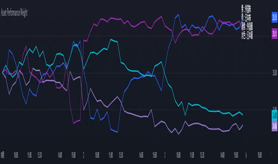
This indicator is a tool that visualizes the relative strength of performance (price change rate) as “weight (allocation ratio)” for **four user-defined stocks**.
By setting any specified past point in time as the baseline (where all symbols are equally weighted at 25%), it aims to provide an intuitive understanding of which symbols outperformed others and attracted capital, or underperformed and saw capital outflows.
**【Default Settings and Application Scenario: Pension Fund Rebalancing Analysis】**
The default settings reference the basic portfolio of Japan's Government Pension Investment Fund (GPIF), configuring four major asset classes: domestic equities, foreign equities, domestic bonds, and foreign bonds. It is known that when market fluctuations cause deviations from this equal-weighted ratio, rebalancing occurs to restore the original ratio (selling assets whose weight has increased and buying assets whose weight has decreased).
Analyzing using this default setting can serve as a reference point for considering **“whether rebalancing sales (or purchases) by pension funds and similar entities are likely to occur in the future.”**
**【Important: Usage Notes】**
The weights shown by this indicator are **theoretical reference values** calculated solely based on performance from the specified start date. Even if large investors conduct significant rebalancing (asset buying/selling) during the period, those transactions themselves are not reflected in this chart's calculations.
Therefore, please understand that the actual portfolio ratios may differ. **Use this solely as a rough guideline. **
#### Key Features
* **Freely configure the 4 assets for analysis:** You can freely set any 4 assets (stocks, indices, currencies, cryptocurrencies, etc.) you wish to compare via the settings screen.
* **Performance-based weight calculation:** Rather than simple price composition ratios, it calculates each asset's price change since the specified start date as a “performance index” and displays each asset's proportion of the total sum.
* **Freely set analysis start date:** You can set any desired starting point for analysis, such as “after the XX shock” or “after earnings announcements,” using the calendar.
* **Multi-Timeframe (MTF) Support:** Independently of the timeframe displayed on the chart, you can freely select the timeframe (e.g., 1-hour, 4-hour, daily) used by the indicator for calculations.
#### Calculation Principle
This indicator calculates weights in the following three steps:
1. **Obtaining the Base Price**
Obtain the closing price for each of the four stocks on the user-set “Start Date for Weight Calculation.” This becomes the **base price** for analysis.
2. **Calculating the Performance Index**
Divide the current price of each stock by the **base price** obtained in Step 1 to calculate the “Performance Index”.
`Performance Index = Current Price ÷ Base Date Price`
This quantifies how many times the current performance has increased compared to the base date performance, which is set to “1”.
3. **Calculating Weights**
Sum the “Performance Indexes” of the four stocks. Then, calculate the percentage contribution of each stock's Performance Index to this total sum and plot it on the chart.
`Weight (%) = (Individual Performance Index ÷ Total Performance Index of 4 Stocks) × 100`
Using this logic, on the analysis start date, all stocks' performance indices are set to “1”, so the weights start equally at 25%.
#### Usage
* **Application Example 1: Market Sentiment Analysis (Using Default Settings)**
Analyze using the default asset classes. By observing the relative strength between “Equities” and “Bonds”, you can assess whether the market is risk-on or risk-off.
* **Application Example 2: Sector/Theme Strength Analysis**
Configure settings for groups like “Top 4 semiconductor stocks” or “4 GAFAM stocks.” Setting the start date to the beginning of the year or earnings season allows you to instantly compare which stocks within the same sector are performing best.
* **Application Example 3: Cryptocurrency Power Map Analysis**
By setting major cryptocurrencies like “BTC, ETH, SOL, ADA,” you can analyze which currencies are attracting market capital.
**【About Legend Display】**
Due to Pine Script specification constraints, the legend on the chart will display fixed names: **“Stock 1” to “Stock 4”. **
Please note that the symbol you entered for “Symbol 1” in the settings corresponds to the “Symbol 1” line on the chart.
#### Settings
* **Symbol 1 to Symbol 4:** Set the four symbols you wish to analyze.
* **Timeframe for Calculation:** Select the timeframe the indicator references when calculating weights.
* **Start Date for Weight Calculation:** This serves as the base date for comparing performance.
#### Disclaimer
This script is solely a tool to assist with market analysis and does not recommend buying or selling any specific financial instruments. Please make all final investment decisions at your own discretion.
-------------------------------------------------------------------------------------------------------------------
**Performance-based Asset Weighting(MTF・シンボル自由設定)**
#### 概要
このインジケーターは、**ユーザーが自由に設定した4つの銘柄**について、パフォーマンス(騰落率)の相対的な強さを「ウェイト(構成比率)」として可視化するツールです。
指定した過去の任意の時点を基準(全銘柄が均等な25%)として、そこからどの銘柄のパフォーマンスが他の銘柄を上回り、資金が向かっているのか、あるいは下回っているのかを直感的に把握することを目的としています。
**【デフォルト設定と活用シナリオ:年金基金のリバランス考察】**
デフォルト設定では、日本の年金積立金管理運用独立行政法人(GPIF)の基本ポートフォリオを参考に、主要4資産クラス(国内株式, 外国株式, 国内債券, 外国債券)が設定されています。市場の変動によってこの均等な比率に乖離が生じると、元の比率に戻すためのリバランス(比率が増えた資産を売り、減った資産を買う)が行われることが知られています。
このデフォルト設定で分析することで、**「今後、年金基金などによるリバランスの売り(買い)が発生する可能性があるか」を考察するための、一つの目安として利用できます。**
**【重要:利用上の注意点】**
このインジケーターが示すウェイトは、あくまで指定した開始日からのパフォーマンスのみを基に算出した**理論上の参考値**です。実際に大口投資家などが途中で大規模なリバランス(資産の売買)を行ったとしても、その取引自体はこのチャートの計算には反映されません。
そのため、実際のポートフォリオ比率とは異なる可能性があることをご理解の上、**あくまで大まかな目安としてご活用ください。**
#### 主な特徴
* **分析対象の4銘柄を自由に設定可能:** 設定画面から、比較したい4つの銘柄(株式、指数、為替、仮想通貨など)を自由に設定できます。
* **パフォーマンス基準のウェイト計算:** 単純な価格の構成比ではなく、指定した開始日からの各銘柄の騰落を「パフォーマンス指数」として算出し、その合計に占める各銘柄の割合を表示します。
* **分析開始日の自由な設定:** 「〇〇ショック後」「決算発表後」など、分析したい任意の時点をカレンダーから設定できます。
* **マルチタイムフレーム(MTF)対応:** チャートに表示している時間足とは別に、インジケーターが計算に使う時間足(1時間足、4時間足、日足など)を自由に選択できます。
#### 計算の原理
このインジケーターは、以下の3ステップでウェイトを算出しています。
1. **基準価格の取得**
ユーザーが設定した「ウェイト計算の開始日」における、4つの各銘柄の終値を取得し、これを分析の**基準価格**とします。
2. **パフォーマンス指数の算出**
現在の各銘柄の価格を、ステップ1で取得した**基準価格**で割ることで、「パフォーマンス指数」を算出します。
`パフォーマンス指数 = 現在の価格 ÷ 基準日の価格`
これにより、基準日のパフォーマンスを「1」とした場合、現在のパフォーマンスが何倍になっているかが数値化されます。
3. **ウェイトの算出**
4つの銘柄の「パフォーマンス指数」の合計値を算出します。そして、合計値に占める各銘柄のパフォーマンス指数の割合(%)を計算し、チャートに描画します。
`ウェイト (%) = (個別のパフォーマンス指数 ÷ 4銘柄のパフォーマンス指数の合計) × 100`
このロジックにより、分析開始日には全銘柄のパフォーマンス指数が「1」となるため、ウェイトは均等に25%からスタートします。
#### 使用方法
* **応用例1:市場のセンチメント分析(デフォルト設定利用)**
デフォルト設定の資産クラスで分析し、「株式」と「債券」の力関係を見ることで、市場がリスクオンなのかリスクオフなのかを判断する材料になります。
* **応用例2:セクター・テーマ別の強弱分析**
設定画面で、例えば「半導体関連の主要4銘柄」や「GAFAMの4銘柄」などを設定します。開始日を年初や決算時期に設定することで、同セクター内でどの銘柄が最もパフォーマンスが良いかを一目で比較できます。
* **応用例3:仮想通貨の勢力図分析**
「BTC, ETH, SOL, ADA」など、主要な仮想通貨を設定することで、市場の資金がどの通貨に向かっているのかを分析できます。
**【凡例の表示について】**
Pine Scriptの仕様上の制約により、チャート上の凡例は**「銘柄1」〜「銘柄4」という固定名で表示されます。**
お手数ですが、設定画面でご自身が「銘柄1」に入力したシンボルが、チャート上の「銘柄1」のラインに対応する、という形でご覧ください。
#### 設定項目
* **銘柄1〜銘柄4:** 分析したい4つのシンボルをそれぞれ設定します。
* **計算に使う時間足:** インジケーターがウェイトを計算する際に参照する時間足を選択します。
* **ウェイト計算の開始日:** パフォーマンスを比較する上での基準日となります。
#### 免責事項
このスクリプトはあくまで市場分析を補助するためのツールであり、特定の金融商品の売買を推奨するものではありません。投資の最終的な判断は、ご自身の責任において行ってください。
Cari dalam skrip untuk "relative strength"
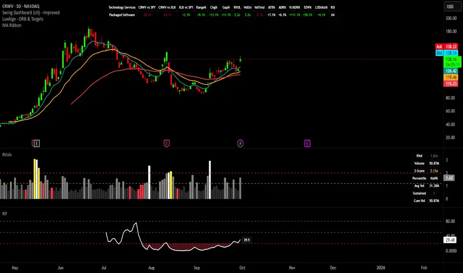
Swing Dashboard - Pro Trader Metrics with MTF & Enhanced VolumeDESCRIPTION:
A comprehensive real-time dashboard designed for swing traders and active investors trading US equities. Displays all critical metrics in one customizable panel overlay - no need to clutter your chart with multiple indicators.
KEY FEATURES:
📊 Relative Strength Analysis:
Stock vs Market (SPY/QQQ/IWM/DIA)
Stock vs Sector (automatic sector ETF detection)
Sector vs Market comparison
Customizable lookback period (5-60 days)
📈 Price & Range Metrics:
Daily range, change, and gap percentages
Distance from SMA20, SMA50, VWAP
52-week position percentage
ATR% and ADR% for volatility assessment
Range/ADR ratio for breakout detection
💪 Advanced Volume Analysis:
RVOL (full day volume vs 20-day average)
Volume Strength (bar-by-bar analysis)
Volume Trend (5-day vs 20-day momentum)
Customizable RVOL alert thresholds
Non-repainting volume calculations
⚙️ Multi-Timeframe (MTF) Mode:
View daily charts with 5-min or 15-min metric updates
Perfect for monitoring positions without switching timeframes
All calculations remain accurate across timeframes
🎨 Fully Customizable:
Choose which metrics to display
9 position options for the dashboard
Adjustable text size and colors
Toggle individual metrics on/off
Sector-specific ETF mapping for accurate RS calculations
TECHNICAL SPECIFICATIONS:
✅ Non-repainting - all calculations use confirmed bar data
✅ No lookahead bias or future data
✅ Optimized for US stocks with proper sector mapping
✅ Works on any timeframe (best on 5m-Daily)
✅ Pine Script v6 with best practices
✅ Handles edge cases and missing data gracefully
IDEAL FOR:
Swing traders monitoring multiple positions
Day traders needing quick metric overview
Investors tracking relative strength and momentum
Anyone who wants institutional-grade metrics in one place
SECTOR ETF MAPPING:
Automatically maps to correct sector ETFs: XLK, XLF, XLV, XLY, XLP, XLE, XLB, XLI, XLRE, XLC, XLU
HOW TO USE:
Green = Positive/Strong | Red = Negative/Weak | White = Neutral
RS > 0 = Outperforming benchmark/sector
RVOL > 1.5x = High volume day
VWAP% negative = Price below VWAP (mean reversion opportunity)
R/ADR > 100% = Extended range (potential exhaustion)
Perfect for traders who need professional-grade analysis without chart clutter.
TAGS:
dashboard, swing, relativestrengrh, sectoranalysis, volume, rvol, multitimeframe, mtf, tradingdashboard, metrics, daytrading, swingtrading, momentum, vwap, atr, volatility, volumeanalysis
Intraday Rising & Reversal ScannerPine Script Description: Intraday Rising & Reversal ScannerThis Pine Script is a TradingView indicator designed to identify stocks with intraday (1-hour timeframe) potential for bullish (rising) or bearish (reversal) movements. It scans for stocks based on user-defined technical criteria, including price change, relative volume, RSI, EMA, ATR, and VWAP. The script plots signals on the chart, displays a summary table, and triggers alerts when conditions are met.FeaturesBullish Signal (Rising Stocks):1H Price Change: > 1% (configurable, e.g., >2% for volatile markets).
Relative Volume: > 2.0 (volume is at least twice the 20-period average).
RSI (14): Between 50 and 70 (strong but not overbought momentum).
Price vs EMA 13: Price above the 13-period EMA (confirms short-term uptrend).
ATR (14): Current ATR above its 20-period average (indicates volatility).
VWAP: Price above VWAP (optional, shown on chart for manual confirmation).
Bearish Signal (Reversal Stocks):1H Price Change: < -1% (configurable, e.g., <-2% for stronger reversals).
Relative Volume: > 2.0 (high volume confirms selling pressure).
RSI (14): > 70 (overbought, increasing reversal likelihood).
Price vs EMA 13: Price below the 13-period EMA (confirms short-term downtrend).
ATR (14): Current ATR above its 20-period average (indicates volatility).
VWAP: Price below VWAP (optional, shown on chart for manual confirmation).
Visualization:Bullish Signal: Green triangle below the bar.
Bearish Signal: Red triangle above the bar.
VWAP: Plotted as a blue line for manual verification.
Table: Displays real-time metrics (Change %, Relative Volume, RSI, Price vs EMA, ATR, VWAP) in the top-right corner, color-coded (green for bullish, red for bearish).
Alerts:Separate alerts for bullish ("Intraday Bullish Signal") and bearish ("Intraday Bearish Signal") conditions.
Customizable alert messages include parameter values for easy tracking.
How It WorksThe script runs on the 1-hour (1H) timeframe, ensuring all calculations are based on hourly data.
Indicators are computed:Change %: Percentage price change over the last hour.
Relative Volume: Current volume divided by the 20-period SMA of volume.
RSI: 14-period Relative Strength Index.
EMA 13: 13-period Exponential Moving Average.
ATR: 14-period Average True Range, compared to its 20-period SMA.
VWAP: Volume Weighted Average Price, plotted for visual confirmation.
Signals are generated when all conditions for either bullish or bearish criteria are met.
A table summarizes key metrics, and alerts can be set up for real-time notifications.
Usage InstructionsApply the Script:Open TradingView’s Pine Editor.
Copy and paste the script.
Click "Add to Chart" and set the chart to the 1-hour (1H) timeframe.
Set Up Alerts:Right-click on the chart > "Add Alert".
Select "Intraday Bullish Signal" or "Intraday Bearish Signal" as the condition.
Configure notifications (e.g., SMS, email, or TradingView alerts).
Manual VWAP Check:VWAP is plotted as a blue line. Verify that the price is above VWAP for bullish signals or below for bearish signals using the table or chart.
To make VWAP a mandatory filter, uncomment the VWAP conditions in the bull_signal and bear_signal definitions.
NASDAQ VWAP Distance Histogram (Multi-Symbol)📊 VWAP Distance Histogram (Multi-Symbol)
This custom indicator plots a histogram of price strength relative to the VWAP (Volume-Weighted Average Price).
The zero line is VWAP.
Histogram bars above zero = price trading above VWAP (strength).
Histogram bars below zero = price trading below VWAP (weakness).
Unlike a standard VWAP overlay, this tool lets you monitor multiple symbols at once and aggregates them into a single, easy-to-read histogram.
🔑 Features
Multi-Symbol Support → Track up to 10 different tickers plus the chart symbol.
Aggregation Options → Choose between average or median deviation across enabled symbols.
Percent or Raw Values → Display distance from VWAP as % of price or raw price points.
Smoothing → Apply EMA smoothing to calm intraday noise.
Color-Coded Histogram → Green above VWAP, red below.
Alerts → Trigger when the aggregate crosses above/below VWAP.
Heads-Up Table → Shows number of symbols tracked and current aggregate reading.
⚡ Use Cases
Market Breadth via VWAP → Monitor whether your basket of stocks is trading above or below VWAP.
Index Substitution → Create your own “mini index” by tracking a hand-picked set of tickers.
Intraday Confirmation → Use aggregate VWAP strength/weakness to confirm entries and exits.
Relative Strength Spotting → Switch on/off specific tickers to see who’s holding above VWAP vs. breaking down.
🛠️ Settings
Include Chart Symbol → Toggle to include the current chart’s ticker.
Smoothing → EMA length (set to 0 to disable).
Percent Mode → Show results as % of price vs. raw difference.
Aggregate Mode → Average or median across all active symbols.
Symbol Slots (S1–S10) → Enter tickers to track alongside the chart.
⚠️ Notes
Works best on intraday charts since VWAP is session-based.
Designed for confirmation, not as a standalone entry/exit signal.
Ensure correct symbol format (e.g., NASDAQ:AAPL if needed).
✅ Tip: Combine this with your regular price action strategy. For example, if your setup triggers long and the histogram is well above zero, that’s added confirmation. If it’s below zero, caution — the basket shows weakness.

EMA-RSI-ADX Trend Bands
📌 EMA-RSI-ADX Trend Bands (ERA Trend Bands)
🔥 Overview
The ERA Trend Bands indicator combines Exponential Moving Average (EMA), Relative Strength Index (RSI), and Average Directional Index (ADX) into a powerful multi-factor trend system.
It helps traders:
Identify trend direction (Bullish / Bearish)
Measure trend strength using EMA deviation bands
Confirm momentum with RSI & ADX filters
Visualize conditions with dynamic colors, labels, tables, and signals
⚡ Key Features
📍 EMA Trend Bands
EMA100 with gradient glow effect showing trend bias
Strength bands around EMA (Very Weak → Hyper levels)
Bands color-coded for bullish/bearish extremes
📊 RSI + ADX Confluence
Bullish Signal: RSI ≥ threshold & ADX ≥ threshold → 🟢
Bearish Signal: RSI ≤ threshold & ADX ≤ threshold → 🔴
Candles recolored when conditions are met
Auto-generated labels show live RSI/ADX values
🧩 Strength Levels
Classifies deviation from EMA into 8 levels:
Neutral → Very Weak → Weak → Moderate → Strong → Very Strong → Extreme → Hyper
Dashboard table shows deviation % ranges & strength colors
Dynamic labels display Trend, Strength, Deviation %, RSI & ADX
🎨 Visual Enhancements
Gradient EMA line with glow effect
Bullish (greens) & bearish (reds) vibrant palettes
Background coloring (optional) based on strength
Symbols & labels for entry confirmation
🎯 How to Use
Trend Direction – EMA color + deviation bands show whether market is bullish or bearish.
Strength Confirmation – Use strength labels & dashboard table to gauge overextension.
Entry Signals – Watch for RSI/ADX confluence (green/red labels on chart).
Exits – Monitor when strength fades back toward Neutral/Weak levels.
⚙️ Settings & Inputs
EMA Settings → Length, Line Width, Gradient Intensity
RSI Settings → Length & Thresholds (Bullish / Bearish)
ADX Settings → Length & Thresholds (Bullish / Bearish)
Bands → Enable/disable EMA deviation bands
Labels/Table → Toggle strength info display
Colors → Fully customizable vibrant palettes
🚨 Alerts & Signals
Bullish Condition → RSI & ADX above thresholds
Bearish Condition → RSI & ADX below thresholds
Visual confirmation with labels, candles, and background
⚠️ Disclaimer
This script is for educational purposes only.
It does not constitute financial advice.
Always backtest and use proper risk management before trading live.
✨ Add EMA-RSI-ADX Trend Bands (ERA Trend Bands) to your chart to trade with clarity, strength, and precision.

Bollinger Bands (SMA 21, 2.618σ)Indicator Description: Bollinger Bands (2.618σ, 21 SMA) + RSI with Fibonacci
This custom indicator combines Bollinger Bands and Relative Strength Index (RSI), enhanced with Fibonacci-based configurations, to provide confluence signals for rejection candles, reversal setups, and continuation patterns.
Bollinger Bands Settings (Customized)
Middle Band → 21-period Simple Moving Average (SMA)
Upper Band → SMA + 2.618 standard deviations
Lower Band → SMA − 2.618 standard deviations
These parameters expand the bands compared to the traditional (20, 2.0) settings, making them better suited for volatility extremes and higher timeframe swing analysis.
Color Scheme
Middle Band = Orange
Upper Band = Red
Lower Band = Green
This color-coding emphasizes key rejection levels visually.
Candle Rejection Logic
The indicator is designed to highlight potential rejection candles when price interacts with the outer Bollinger Bands:
At the Upper Band, rejection signals suggest overextension and potential downside reaction.
At the Lower Band, rejection signals suggest oversold conditions and potential upside reaction.
Rejection Candle Types Tracked
Hammer (bullish reversal, lower rejection wick at bottom band)
Inverted Hammer (bearish reversal, upper rejection wick at top band)
Doji candles (indecision at band extremes)
Double Top formations near the upper band
Double Bottom formations near the lower band
Relative Strength Index (RSI) Settings
RSI is configured with Fibonacci retracement levels instead of traditional 30/70 thresholds.
Fibonacci sequence levels used include:
23.6% (0.236)
38.2% (0.382)
50% (0.5)
61.8% (0.618)
78.6% (0.786)
This alignment with Fibonacci ratios provides deeper market structure insights into momentum strength and exhaustion points.
Trading Confluence Zones
Upper Band + RSI at 0.618–0.786 zone → High probability bearish rejection.
Lower Band + RSI at 0.236–0.382 zone → High probability bullish reversal.
Band interaction + Doji or Hammer candles → Stronger signal confirmation.
Use Cases
Identifying trend exhaustion when price repeatedly fails to break above the upper band.
Spotting accumulation or distribution phases when price consolidates around Fibonacci-based RSI zones.
Detecting false breakouts when candle patterns (like Doji or Inverted Hammer) occur beyond the bands.
Why 2.618 Deviation & 21 SMA?
Standard Bollinger Bands (20, 2.0) capture ~95% of price action.
By widening to 2.618σ, we target extreme volatility outliers — areas where reversals are statistically more likely.
A 21-period SMA aligns better with common cycle lengths (3 trading weeks on daily charts) and Fibonacci-related time cycles.
Practical Strategy
Step 1: Watch when price touches or pierces the upper/lower band.
Step 2: Check for candle rejection patterns (Hammer, Inverted Hammer, Doji, Double Top/Bottom).
Step 3: Confirm with RSI Fibonacci levels for confluence.
Step 4: Trade with the prevailing trend or look for reversal setups if multiple confluence factors align.
Cautions
Not all touches of the bands signal reversals — strong trends can ride along the bands for extended periods.
Always combine with price action structure, volume, and higher timeframe trend bias.
📌 Summary
This indicator blends volatility-based bands with Fibonacci momentum analysis and classical candle rejection patterns. The combination of Bollinger Bands (21, 2.618σ) and RSI Fibonacci levels helps traders detect high-probability rejection zones, reversal opportunities, and overextended conditions with improved accuracy over traditional default settings.

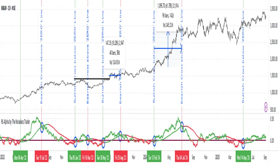
RS Alpha by The Noiseless TraderRS Alpha by The Noiseless Trader plots a clean, benchmark‑relative strength line for any symbol and (optionally) a mean line to assess trend and momentum in relative performance. It’s designed for uncluttered, professional RS analysis and works across any timeframe.
Compare any symbol vs a benchmark (default: NSE:NIFTY).
Optional log‑normalized RS for return‑aware comparisons.
Optional RS Mean with trend coloring (rising/falling).
Optional RS Trend zero‑line coloring based on short‑range slope.
Lightweight alerts for rising/falling RS mean.
Tip: Use RS to identify leaders (RS > 0 with rising mean) and laggards (RS < 0 with falling mean), then align setups with your price action rules.
Reading the indicator
Leadership: RS > 0 and RS Mean rising → outperformance vs benchmark.
Weakness: RS < 0 and RS Mean falling → underperformance vs benchmark.
Inflections: Watch RS crossing above/below its Mean for early shifts.
Zero‑line context: With RS Trend on, the zero line subtly reflects short‑term slope (green for positive, maroon for negative).
Alerts
Rising Strength – RS Mean turning/remaining upward.
Declining Strength – RS Mean turning/remaining downward.
(Use these as context; execute entries on your price‑action rules.)
Best practices
Pair RS with your trend/structure rules (e.g., higher highs + RS leadership).
For sectors/baskets, keep the Comparative Symbol consistent to rank peers.
Log‑normalized RS helps when comparing assets with very different volatilities or large base effects.
Test multiple length and Mean settings; 60 is a balanced default for swing/positional work.
Credits
Original concept & code: © bharatTrader
Modifications & refinements: The Noiseless Trader
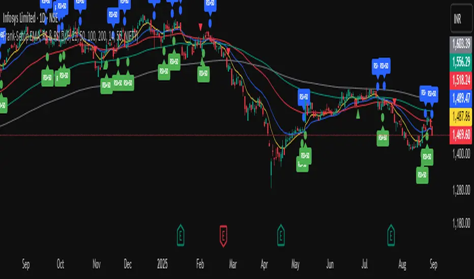
Frank-Setup EMA, RS & RSI ✅It is a clean and simple indicator designed to identify weakness in stocks using two proven methods: RSI and Relative Strength (RS) vs. a benchmark (e.g., NIFTY).
🔹 Features
RSI Weakness Signals
Plots when RSI crosses below 50 (weakness begins).
Plots when RSI moves back above 50 (weakness ends).
Relative Strength (RS) vs Benchmark
Compares stock performance to a chosen benchmark.
Signals when RS drops below 1 (stock underperforming).
Signals when RS recovers above 1 (strength resumes).
Clear Visual Markers
Circles for RSI signals.
Triangles for RS signals.
Optional RSI labels for clarity.
Built-in Alerts
Get notified instantly when RSI or RS weakness starts or ends.
No need to constantly watch charts.
🎯 Use Case
This tool is built for traders who want to:
Spot shorting opportunities when a stock shows weakness.
Track underperformance vs. the index.
Manage risk by exiting longs when weakness appears.
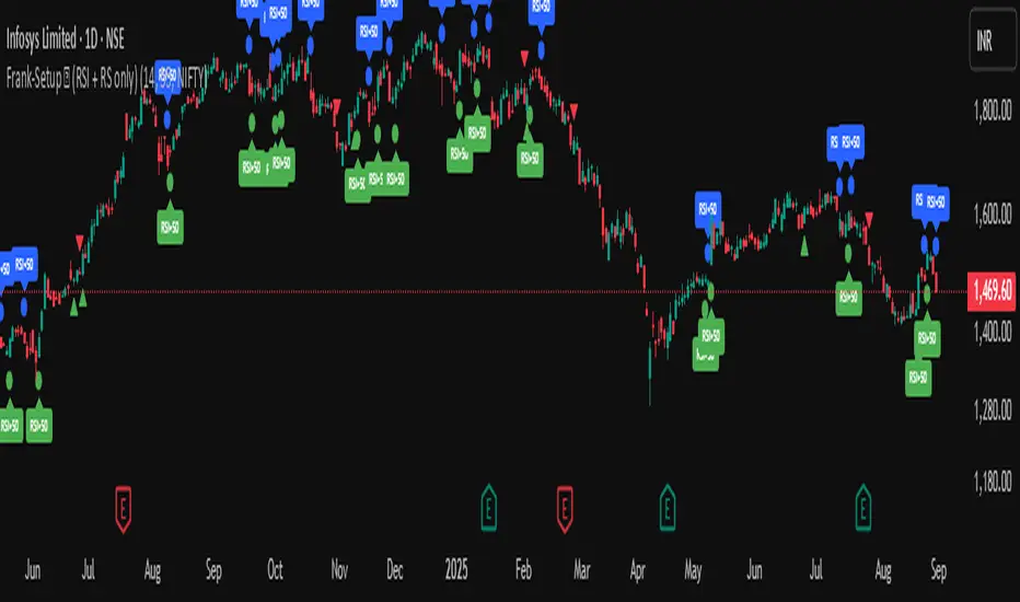
Frank-Setup ✅ (RSI + RS only)Frank-Shorting Setup ✅ is an indicator designed to help traders spot weakness in a stock by combining RSI and Relative Strength (RS) analysis.
🔹 Key Features
RSI Weakness Signals
Marks when RSI falls below 50 (downside pressure begins).
Marks when RSI moves back above 50 (weakness ends).
Relative Strength (RS) vs Benchmark
Compares stock performance to a benchmark (e.g., NIFTY).
Signals when RS drops below 1 (stock underperforming).
Signals when RS moves back above 1 (strength resumes).
Clear Chart Markings
Circles for RSI signals.
Triangles for RS signals.
Optional labels for extra clarity.
Alerts Built-In
Get notified when RSI or RS weakness starts/ends.
No need to monitor charts all the time

Frank-Shorting Setup ✅ (RSI + RS only)An indicator designed to help traders spot weakness in a stock by combining RSI and Relative Strength (RS) analysis.
🔹 Key Features
RSI Weakness Signals
Marks when RSI falls below 50 (downside pressure begins).
Marks when RSI moves back above 50 (weakness ends).
Relative Strength (RS) vs Benchmark
Compares stock performance to a benchmark (e.g., NIFTY).
Signals when RS drops below 1 (stock underperforming).
Signals when RS moves back above 1 (strength resumes).
Clear Chart Markings
Circles for RSI signals.
Triangles for RS signals.
Optional labels for extra clarity.
Alerts Built-In
Get notified when RSI or RS weakness starts/ends.
No need to monitor charts all the time
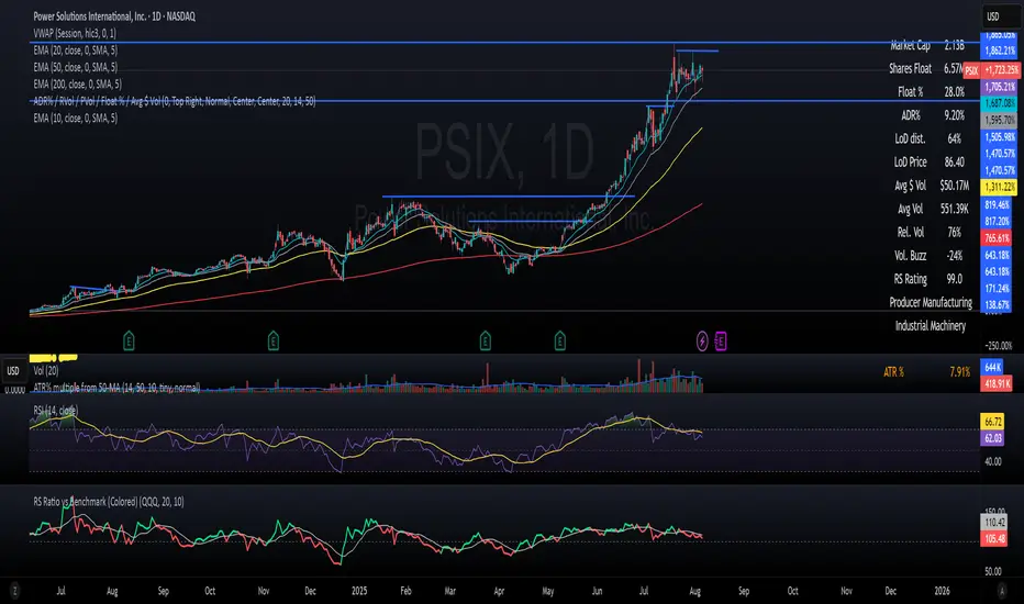
RS Ratio vs Benchmark (Colored)📈 RS Ratio vs Benchmark (with Color Change)
A simple but powerful tool to track relative strength against a benchmark like QQQ, SPY, or any other ETF.
🔍 What it Shows
RS Ratio (orange line): Measures how strong a stock is relative to a benchmark.
Moving Average (teal line): Smooths out RS to show trend direction.
Color-coded RS Line:
🟢 Green = RS is above its moving average → strength is increasing.
🔴 Red = RS is below its moving average → strength is fading.
📊 How to Read It
Above 100 = Stock is outperforming the benchmark.
Below 100 = Underperforming.
Rising & Green = Strongest signal — accelerating outperformance.
Above 100 but Red = Consolidating or losing momentum — potential rest period.
Crosses below 100 = Warning sign — underperformance.
✅ Best Uses
Spot leading stocks with strong momentum vs QQQ/SPY.
Identify rotation — when strength shifts between sectors.
Time entries and exits based on RS trends and crossovers.
MSTY-WNTR Rebalancing SignalMSTY-WNTR Rebalancing Signal
## Overview
The **MSTY-WNTR Rebalancing Signal** is a custom TradingView indicator designed to help investors dynamically allocate between two YieldMax ETFs: **MSTY** (YieldMax MSTR Option Income Strategy ETF) and **WNTR** (YieldMax Short MSTR Option Income Strategy ETF). These ETFs are tied to MicroStrategy (MSTR) stock, which is heavily influenced by Bitcoin's price due to MSTR's significant Bitcoin holdings.
MSTY benefits from upward movements in MSTR (and thus Bitcoin) through a covered call strategy that generates income but caps upside potential. WNTR, on the other hand, provides inverse exposure, profiting from MSTR declines but losing in rallies. This indicator uses Bitcoin's momentum and MSTR's relative strength to signal when to hold MSTY (bullish phases), WNTR (bearish phases), or stay neutral, aiming to optimize returns by switching allocations at key turning points.
Inspired by strategies discussed in crypto communities (e.g., X posts analyzing MSTR-linked ETFs), this indicator promotes an active rebalancing approach over a "set and forget" buy-and-hold strategy. In simulated backtests over the past 12 months (as of August 4, 2025), the optimized version has shown potential to outperform holding 100% MSTY or 100% WNTR alone, with an illustrative APY of ~125% vs. ~6% for MSTY and ~-15% for WNTR in one scenario.
**Important Disclaimer**: This is not financial advice. Past performance does not guarantee future results. Always consult a financial advisor. Trading involves risk, and you could lose money. The indicator is for educational and informational purposes only.
## Key Features
- **Momentum-Based Signals**: Uses a Simple Moving Average (SMA) on Bitcoin's price to detect bullish (price > SMA) or bearish (price < SMA) trends.
- **RSI Confirmation**: Incorporates MSTR's Relative Strength Index (RSI) to filter signals, avoiding overbought conditions for MSTY and oversold for WNTR.
- **Visual Cues**:
- Green upward triangle for "Hold MSTY".
- Red downward triangle for "Hold WNTR".
- Yellow cross for "Switch" signals.
- Background color: Green for MSTY, red for WNTR.
- **Information Panel**: A table in the top-right corner displays real-time data: BTC Price, SMA value, MSTR RSI, and current Allocation (MSTY, WNTR, or Neutral).
- **Alerts**: Configurable alerts for holding MSTY, holding WNTR, or switching.
- **Optimized Parameters**: Defaults are tuned (SMA: 10 days, RSI: 15 periods, Overbought: 80, Oversold: 20) based on simulations to reduce whipsaws and capture trends effectively.
## How It Works
The indicator's logic is straightforward yet effective for volatile assets like Bitcoin and MSTR:
1. **Primary Trigger (Bitcoin Momentum)**:
- Calculate the SMA of Bitcoin's closing price (default: 10-day).
- Bullish: Current BTC price > SMA → Potential MSTY hold.
- Bearish: Current BTC price < SMA → Potential WNTR hold.
2. **Secondary Filter (MSTR RSI Confirmation)**:
- Compute RSI on MSTR stock (default: 15-period).
- For bullish signals: If RSI > Overbought (80), signal Neutral (avoid overextended rallies).
- For bearish signals: If RSI < Oversold (20), signal Neutral (avoid capitulation bottoms).
3. **Allocation Rules**:
- Hold 100% MSTY if bullish and not overbought.
- Hold 100% WNTR if bearish and not oversold.
- Neutral otherwise (e.g., during choppy or extreme markets) – consider holding cash or avoiding trades.
4. **Rebalancing**:
- Switch signals trigger when the hold changes (e.g., from MSTY to WNTR).
- Recommended frequency: Weekly reviews or on 5% BTC moves to minimize trading costs (aim for 4-6 trades/year).
This approach leverages Bitcoin's influence on MSTR while mitigating the risks of MSTY's covered call drag during downtrends and WNTR's losses in uptrends.
## Setup and Usage
1. **Chart Requirements**:
- Apply this indicator to a Bitcoin chart (e.g., BTCUSD on Binance or Coinbase, daily timeframe recommended).
- Ensure MSTR stock data is accessible (TradingView supports it natively).
2. **Adding to TradingView**:
- Open the Pine Editor.
- Paste the script code.
- Save and add to your chart.
- Customize inputs if needed (e.g., adjust SMA/RSI lengths for different timeframes).
3. **Interpretation**:
- **Green Background/Triangle**: Allocate 100% to MSTY – Bitcoin is in an uptrend, MSTR not overbought.
- **Red Background/Triangle**: Allocate 100% to WNTR – Bitcoin in downtrend, MSTR not oversold.
- **Yellow Switch Cross**: Rebalance your portfolio immediately.
- **Neutral (No Signal)**: Panel shows "Neutral" – Hold cash or previous position; reassess weekly.
- Monitor the panel for key metrics to validate signals manually.
4. **Backtesting and Strategy Integration**:
- Convert to a strategy script by changing `indicator()` to `strategy()` and adding entry/exit logic for automated testing.
- In simulations (e.g., using Python or TradingView's backtester), it has outperformed buy-and-hold in volatile markets by ~100-200% relative APY, but results vary.
- Factor in fees: ETF expense ratios (~0.99%), trading commissions (~$0.40/trade), and slippage.
5. **Risk Management**:
- Use with a diversified portfolio; never allocate more than you can afford to lose.
- Add stop-losses (e.g., 10% trailing) to protect against extreme moves.
- Rebalance sparingly to avoid over-trading in sideways markets.
- Dividends: Reinvest MSTY/WNTR payouts into the current hold for compounding.
## Performance Insights (Simulated as of August 4, 2025)
Based on synthetic backtests modeling the last 12 months:
- **Optimized Strategy APY**: ~125% (by timing switches effectively).
- **Hold 100% MSTY APY**: ~6% (gains from BTC rallies offset by downtrends).
- **Hold 100% WNTR APY**: ~-15% (losses in bull phases outweigh bear gains).
In one scenario with stronger volatility, the strategy achieved ~4533% APY vs. 10% for MSTY and -34% for WNTR, highlighting its potential in dynamic markets. However, these are illustrative; real results depend on actual BTC/MSTR movements. Test thoroughly on historical data.
## Limitations and Considerations
- **Data Dependency**: Relies on accurate BTC and MSTR data; delays or gaps can affect signals.
- **Market Risks**: Bitcoin's volatility can lead to false signals (whipsaws); the RSI filter helps but isn't perfect.
- **No Guarantees**: This indicator doesn't predict the future. MSTR's correlation to BTC may change (e.g., due to regulatory events).
- **Not for All Users**: Best for intermediate/advanced traders familiar with ETFs and crypto. Beginners should paper trade first.
- **Updates**: As of August 4, 2025, this is version 1.0. Future updates may include volume filters or EMA options.
If you find this indicator useful, consider leaving a like or comment on TradingView. Feedback welcome for improvements!

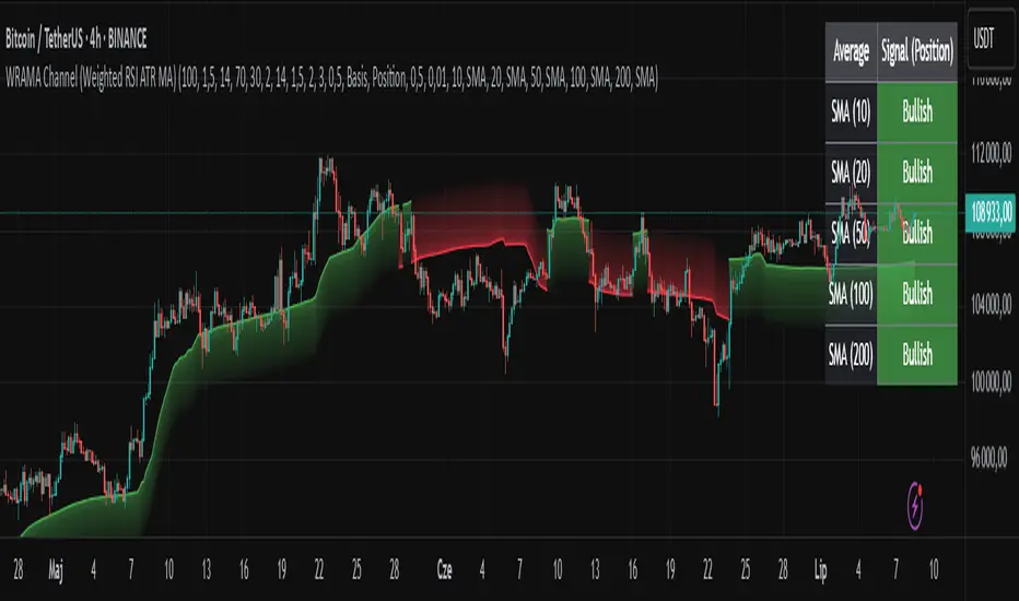
WRAMA Channel (Weighted RSI ATR MA)OVERVIEW
The WRAMA Channel (Weighted RSI ATR MA) is an advanced technical analysis tool designed to react more quickly to price movements compared to indicators using conventional moving averages. It combines the Relative Strength Index (RSI), Average True Range (ATR), and a weighted moving average, resulting in the WRAMA. This indicator forms a dynamic price channel based on a weighted average that incorporates both trend strength (via RSI) and market volatility (via ATR). It helps traders identify trends, potential reversals, and breakout signals, while offering broad customization options.
Key Features
WRAMA Price Channel:
Generates a dynamic channel around the weighted moving average (WRAMA), adapting to market volatility and momentum, similar to Bollinger Bands. Users are encouraged to adjust channel width and length according to their strategy.
The upper and lower channel bands are calculated based on a percentage deviation from the baseline line.
The channel fill color changes depending on the price's position relative to the baseline (green above, red below), with an optional gradient for better visualization.
Weighted Moving Average (WRAMA):
WRAMA is a custom weighted moving average (MA1), where closing prices are weighted based on RSI and ATR, allowing it to dynamically adapt to market conditions.
Baseline: The WRAMA line calculated over a user-defined period.
WRAMA Calculation:
RSI Weight: Based on RSI value. When RSI is in extreme zones (below the lower threshold or above the upper threshold), an extreme weight is applied. Otherwise, the weight is based on the squared RSI value divided by 100, raised to a power defined by the rsi_weight_factor.
ATR Weight: Based on the ATR-to-average-ATR ratio. If ATR exceeds a threshold (atr_threshold × avg_atr), an extreme weight is applied. Otherwise, the weight is based on the squared ratio of ATR to average ATR, raised to the power of the atr_weight_factor.
Combined Weight: RSI and ATR weights are combined using a rsi_atr_balance parameter. Final weight = RSI weight × balance + ATR weight × (1 - balance).
WRAMA Calculation: The closing price is multiplied by the combined weight. The result is averaged over the ma_length period and divided by the average of the weights, forming the WRAMA line. For current WRAMA (ma_length = 1), the calculation simplifies to a single weighted price.
Additional Moving Averages:
For additional confirmations, the indicator supports up to five moving averages (MA1–MA5) with various types (SMA, EMA, WMA, HMA, ALMA) and customizable periods.
All additional MAs are calculated based on WRAMA or its baseline, ensuring consistency and enabling deeper analysis within a unified methodology. MA trend directions can be tracked in a built-in signal table.
Trading Signals:
Breakout Signals: Breakouts above/below the channel are optionally marked with triangle shapes (green for bullish, red for bearish).
MA Signals: Price position relative to MAs or their slope generates bullish/bearish signals. These are optionally visualized with default triangles (green up, red down).
A signal table in the top-right corner summarizes the status of each moving average – bullish, bearish, or neutral.
Customization Options
Channel Settings:
MA Period: Length of the WRAMA baseline (default: 100).
Channel Deviation : Percentage offset from the baseline for upper/lower bands (default: 1.5%).
RSI Settings:
RSI Period: Length of the RSI calculation (default: 14).
RSI Upper/Lower Threshold: Overbought/oversold levels (default: 70/30).
RSI Weight Factor: Influence of RSI on weighting (default: 2.0).
ATR Settings:
ATR Period: ATR calculation length (default: 14).
ATR Threshold: Volatility threshold as a multiple of average ATR (default: 1.5).
ATR Weight Factor: Influence of ATR on weighting (default: 2.0).
RSI & ATR Combined:
Extreme Weight: Weight applied in extreme RSI/ATR conditions (default: 3.0).
RSI/ATR Balance: Balance between RSI and ATR influence (default: 0.5).
Signal Settings:
Show Breakout Signals: Enable/disable breakout triangles.
Show MA Signals: Enable/disable MA-based signals.
MA Signal Source: Choose between current WRAMA or baseline.
MA Signal Analysis: Based on price position or slope.
Neutral Threshold : Minimum distance from MA for signal neutrality (default: 0.5%).
Minimum MA Slope : Minimum slope for trend direction signals (default: 0.01%).
Moving Averages (MA1–MA5):
Options to enable/disable, select type (SMA, EMA, WMA, HMA, ALMA), set period length, and choose color.
Style Settings:
Gradient Fill: Enable/disable gradient coloring within the channel.
Show Baseline: Enable/disable WRAMA baseline visibility.
Colors: Customize line, fill, and signal colors.
Use Cases
Trend Identification: The WRAMA channel highlights trend direction and potential reversal zones when price contacts the channel edges.
Breakout Signals: Channel breakouts may indicate trend shifts or momentum surges.
MA Analysis: The signal table provides a clear summary of market direction (bullish, bearish, or neutral) based on selected moving averages.
Trading Strategies: Suitable for trend-following, mean-reversion, and scalping strategies, depending on user preferences and settings.
Notes
The indicator offers a high degree of flexibility, making it adaptable to various trading styles, instruments, and timeframes.
It is recommended to adjust channel length and width to fit your trading strategy.
Backtesting settings on historical data is advised to optimize parameters for a specific strategy and market.
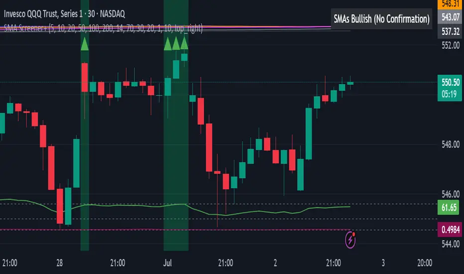
All SMAs Bullish/Bearish Screener (Enhanced)All SMAs Bullish/Bearish Screener Enhanced: Uncover High-Conviction Trend Alignments with Confidence
Description:
Are you ready to elevate your trading from mere guesswork to precise, data-driven decisions? The "All SMAs Bullish/Bearish Screener Enhanced" is not just another indicator; it's a sophisticated, yet user-friendly, trend-following powerhouse designed to cut through market noise and pinpoint high-probability trading opportunities. Built on the foundational strength of comprehensive Moving Average confluence and fortified with critical confirmation signals from Momentum, Volume, and Relative Strength, this script empowers you to identify truly robust trends and manage your trades with unparalleled clarity.
The Power of Multi-Factor Confluence: Beyond Simple Averages
In the unpredictable world of financial markets, true strength or weakness is rarely an isolated event. It's the harmonious alignment of multiple technical factors that signals a high-conviction move. While our original "All SMAs Bullish/Bearish Screener" intelligently identified stocks where price was consistently above or below a full spectrum of Simple Moving Averages (5, 10, 20, 50, 100, 200), this Enhanced version takes it a crucial step further.
We've integrated a powerful three-pronged confirmation system to filter out weaker signals and highlight only the most compelling setups:
Momentum (Rate of Change - ROC): A strong trend isn't just about price direction; it's about the speed and intensity of that movement. Positive momentum confirms that buyers are still aggressively pushing price higher (for bullish signals), while negative momentum validates selling pressure (for bearish signals).
Volume: No trend is truly trustworthy without the backing of smart money. Above-average volume accompanying an "All SMAs" alignment signifies strong institutional participation and conviction behind the move. It separates genuine trend starts from speculative whims.
Relative Strength Index (RSI): This versatile oscillator ensures the trend isn't just "there," but that it's developing healthily. We use RSI to confirm a bullish bias (above 50) or a bearish bias (below 50), adding another layer of confidence to the direction.
When the price aligns above ALL six critical SMAs, and is simultaneously confirmed by robust positive momentum, healthy volume, and a bullish RSI bias, you have an exceptionally strong "STRONGLY BULLISH" signal. This confluence often precedes sustained upward moves, signaling prime accumulation phases. Conversely, a "STRONGLY BEARISH" signal, where price is below ALL SMAs with negative momentum, confirming volume, and a bearish RSI bias, indicates powerful distribution and potential for significant downside.
How to Use This Enhanced Screener:
Add to Chart: Go to TradingView's Pine Editor, paste the script, and click "Add to Chart."
Customize Parameters: Fine-tune the lengths of your SMAs, RSI, Momentum, and Volume averages via the indicator's settings. Experiment to find what best suits your trading style and the assets you trade.
Choose Your Timeframe Wisely:
Daily (1D) and 4-Hour (240 min) are highly recommended. These timeframes cut through intraday noise and provide more reliable, actionable signals for swing and position trading.
Shorter timeframes (e.g., 15min, 60min) can be used by advanced day traders for very short-term entries, but be aware of increased volatility and noise.
Visual Confirmation:
Green/Red Triangles: Appear on your chart, indicating confirmed bullish or bearish signals.
Background Color: The chart background will subtly turn lime green for "STRONGLY BULLISH" and red for "STRONGLY BEARISH" conditions.
On-Chart Status Table: A clear table displays the current signal status ("STRONGLY BULLISH/BEARISH," or "SMAs Mixed") for immediate feedback.
Set Up Alerts (Your Primary Screener Tool): This is the game-changer! Create custom alerts on TradingView based on the "Confirmed Bullish Trade" and "Confirmed Bearish Trade" conditions. Receive instant notifications (email, pop-up, mobile) for any stock in your watchlist that meets these stringent criteria. This allows you to scan the entire market effortlessly and act decisively.
Strategic Stop-Loss Placement: The Trader's Lifeline
Even the most robust signals can fail. Protecting your capital is paramount. For this trend-following strategy, your stop-loss should be placed where the underlying trend structure is broken.
For a "STRONGLY BULLISH" Trade: Place your stop-loss just below the most recent significant swing low (higher low). This is the last point where buyers stepped in to support the price. If price breaks below this, your bullish thesis is invalidated.
For a "STRONGLY BEARISH" Trade: Place your stop-loss just above the most recent significant swing high (lower high). If price breaks above this, your bearish thesis is invalidated.
Alternatively, consider placing your stop-loss just below the 20-period SMA (for bullish trades) or above the 20-period SMA (for bearish trades). A significant close beyond this intermediate-term average often indicates a critical shift in momentum. Always ensure your chosen stop-loss adheres to your pre-defined risk per trade (e.g., 1-2% of capital).
Disciplined Profit Booking: Maximizing Gains
Just as important as knowing when you're wrong is knowing when to take profits.
Trailing Stop-Loss: As your trade moves into profit, trail your stop-loss upwards (for longs) or downwards (for shorts). You can trail it using:
Previous Swing Lows/Highs: Move your stop to just below each new higher low (for longs) or just above each new lower high (for shorts).
A Moving Average (e.g., 10-period or 20-period SMA): If price closes below your chosen trailing SMA, exit. This allows you to ride the trend while protecting accumulated profits.
Target Levels: Identify potential resistance levels (for longs) or support levels (for shorts) using pivot points, previous highs/lows, or Fibonacci extensions. Consider taking partial profits at these levels and letting the rest run with a trailing stop.
Loss of Confluence: If the "STRONGLY BULLISH/BEARISH" condition ceases to be met (e.g., RSI crosses below 50, or volume drops significantly), this can be a signal to reduce or exit your position, even if your stop-loss hasn't been hit.
The "All SMAs Bullish/Bearish Screener Enhanced" is your comprehensive partner in navigating the markets. By combining robust trend identification with critical confirmation signals and disciplined risk management, you're equipped to make smarter, more confident trading decisions. Add it to your favorites and unlock a new level of precision in your trading journey!
#PineScript #TradingView #SMA #MovingAverage #TrendFollowing #StockScreener #TechnicalAnalysis #Bullish #Bearish #QQQ #Momentum #Volume #RSI #SPY #TradingStrategy #Enhanced #Signals #Analysis #DayTrading #SwingTrading
RSI Buy Sell Signals[RanaAlgo]Overview
This Premium RSI with Enhanced Signals builds upon the classic Relative Strength Index by incorporating multiple confirmation filters and visual enhancements to improve signal reliability. The indicator goes beyond basic overbought/oversold levels by adding volume confirmation, trend alignment, and peak detection logic.
Key Features
Enhanced Signal Detection
Peak Strength Filter: Requires RSI movements to meet minimum strength criteria (configurable from 1-5 bars)
Volume Confirmation: Optional volume filter to ensure signals occur with above-average trading activity
Trend Alignment: Optional trend confirmation that checks price position relative to 20-period EMA
Visual Improvements
Dynamic coloring of RSI line (green in oversold, red in overbought)
Customizable reference lines and zones
Clear buy/sell signals with triangle markers
Comprehensive info panel showing current RSI status
Alert Capabilities
Ready-to-use alert conditions for both buy and sell signals
Visual and audible alerts when signals trigger
How It Works
Core RSI Calculation: Uses standard RSI formula with configurable length (default 14)
Signal Generation:
Buy signals require either:
RSI rising from oversold with volume/trend confirmation (when enabled)
Simple crossover above oversold level (when filters disabled)
Sell signals require either:
RSI falling from overbought with volume/trend confirmation
Simple crossunder below overbought level
Additional Filters:
Minimum peak strength prevents weak, insignificant movements from generating signals
Volume filter helps confirm institutional participation
Trend filter aligns signals with broader price direction
Usage Instructions
Apply to any chart timeframe (works best on 1H or higher)
Configure settings in the input panel:
Adjust RSI length if needed
Set overbought/oversold levels (default 70/30)
Enable/disable volume and trend filters
Customize visual elements
Signals appear as triangles below/above the RSI line
Use alerts to get notified of new signals
Differentiation from Standard RSI
This indicator adds several layers of confirmation that aren't present in the basic RSI:
Multi-bar momentum requirement for peaks/troughs
Volume validation option
Trend confirmation option
Smoothed RSI line for cleaner visualization
Comprehensive info panel with current status
The combination of these features helps filter out false signals that commonly occur with traditional RSI implementations.

CAN INDICATORCAN Moving Averages Indicator - Feature Guide
1. Multiple Moving Averages (20 MAs)
- Supports up to 20 individual moving averages
- Each MA can be independently configured:
- Enable/Disable toggle
- Length (period) setting
- Type selection (SMA, EMA, DEMA, VWMA, RMA, WMA)
- Color customization
- Individual timeframe settings when global timeframe is disabled
Pre-configured MA Settings:
1. MA1-8: SMA type
- Lengths: 20, 50, 100, 200, 365, 489, 600, 1460
2. MA9-20: EMA type
- Lengths: 30, 60, 120, 240, 300, 400, 500, 700, 800, 900, 1000, 2000
2. Global Timeframe Settings
Location: Global Settings group
Features:
- Use Global Timeframe: Toggle to use one timeframe for all MAs
- Global Timeframe: Select the timeframe to apply globally
3. Label Display Options
Location: Main Inputs section
Controls:
- Show MA Type: Display MA type (SMA, EMA, etc.)
- Show MA Length: Display period length
- Show Resolution: Display timeframe
- Label Offset: Adjust label position
4. Cross Alerts System
Location: Cross Alerts group
Features:
1. Price Crosses:
- Alerts when price crosses any selected MA
- Select MA to monitor (1-20)
- Triggers on crossover/crossunder
2. MA Crosses:
- Alerts when one MA crosses another
- Select fast MA (1-20)
- Select slow MA (1-20)
- Triggers on crossover/crossunder
5. Relative Strength (RS) Analysis
Location: Relative Strength group
Features:
- Select any MA to monitor (1-20)
- Compares MA to its own average
- Adjustable RS Length (default 14)
- Visual feedback via background color:
- Green: MA above its average (uptrend)
- Red: MA below its average (downtrend)
- Customizable colors and transparency
6. Moving Average Types Available
1. **SMA** (Simple Moving Average)
- Equal weight to all prices
2. **EMA** (Exponential Moving Average)
- More weight to recent prices
3. **DEMA** (Double Exponential Moving Average)
- Reduced lag compared to EMA
4. **VWMA** (Volume Weighted Moving Average)
- Incorporates volume data
5. **RMA** (Running Moving Average)
- Smoother than EMA
6. **WMA** (Weighted Moving Average)
- Linear weight distribution
Usage Tips
1. **For Trend Following:**
- Enable longer-period MAs (MA4-MA8)
- Use cross alerts between long-term MAs
- Monitor RS for trend strength
2. **For Short-term Trading:**
- Focus on shorter-period MAs (MA1-MA3, MA9-MA11)
- Enable price cross alerts
- Use multiple timeframe analysis
3. **For Multiple Timeframe Analysis:**
- Disable global timeframe
- Set different timeframes for each MA
- Compare MA relationships across timeframes
4. **For Performance:**
- Disable unused MAs
- Limit active alerts to necessary pairs
- Use RS selectively on key MAs

RSI Candlestick Oscillator [LuxAlgo]The RSI Candlestick Oscillator displays a traditional Relative Strength Index (RSI) as candlesticks. This indicator references OHLC data to locate each candlestick point relative to the current RSI Value, leading to a more accurate representation of the Open, High, Low, and Close price of each candlestick in the context of RSI.
In addition to the candlestick display, Divergences are detected from the RSI candlestick highs and lows and can be displayed over price on the chart.
🔶 USAGE
Translating candlesticks into the RSI oscillator is not a new concept and has been attempted many times before. This indicator stands out because of the specific method used to determine the candlestick OHLC values. When compared to other RSI Candlestick indicators, you will find that this indicator clearly and definitively correlates better to the on-chart price action.
Traditionally, the RSI indicator is simply one running value based on (typically) the close price of the chart. By introducing high, low, and open values into the oscillator, we can better gauge the specific price action throughout the intrabar movements.
Interactions with the RSI levels can now take multiple forms, whether it be a full-bodied breakthrough or simply a wick test. Both can provide a new analysis of price action alongside RSI.
An example of wick interactions and full-bodied interactions can be seen below.
As a result of the candlestick display, divergences become simpler to spot. Since the candlesticks on the RSI closely resemble the candlesticks on the chart, when looking for divergence between the chart and RSI, it is more obvious when the RSI and price are diverging.
The divergences in this indicator not only show on the RSI oscillator, but also overlay on the price chart for clearer understanding.
🔹 Filtering Divergence
With the candlesticks generating high and low RSI values, we can better sense divergences from price, since these points are generally going to be more dramatic than the (close) RSI value.
This indicator displays each type of divergence:
Bullish Divergence
Bearish Divergence
Hidden Bullish Divergence
Hidden Bearish Divergence
From these, we get many less-than-useful indications, since every single divergence from price is not necessarily of great importance.
The Divergence Filter disregards any divergence detected that does not extend outside the RSI upper or lower values.
This does not replace good judgment, but this filter can be helpful in focusing attention towards the extremes of RSI for potential reversal spotting from divergence.
🔶 DETAILS
In order to get the desired results for a display that resembles price action while following RSI, we must scale. The scaling is the most important part of this indicator.
To summarize the process:
Identify a range on Price and RSI
Consider them as equal to create a scaling factor
Use the scaling factor to locate RSI's "Price equivalent" Upper, Lower, & Mid on the Chart
Use those prices (specifically the RSI Mid) to check how far each OHLC value lies from it
Use those differences to translate the price back to the RSI Oscillator, pinning the OHLC values at their relative location to our anchor (RSI Mid)
🔹 RSI Channel
To better understand, and for your convenience, the indicator includes the option to display the RSI Channel on the chart. This channel helps to visualize where the scaled RSI values are relative to price.
If you analyze the RSI channel, you are likely to notice that the price movement throughout the channel matches the same movement witnessed in the RSI Oscillator below. This makes sense since they are the exact same thing displayed on different scales.
🔹 Scaling the Open
While the scaling method used is important, and provides a very close view of the real price bar's relative locations on the RSI oscillator… It is designed for a single purpose.
The scaling does NOT make the price candles display perfectly on the RSI oscillator.
The largest place where this is noticeable is with the opening of each candle.
For this reason, we have included a setting that modifies the opening of each RSI candle to be more accurate to the chart's price candles.
This setting positions the current bar's opening RSI candlestick value accurately relative to the price's open location to the previous closing price. As seen below.
🔶 SETTINGS
🔹 RSI Candles
RSI Length: Sets the Length for the RSI Oscillator.
Overbought/Oversold Levels: Sets the Overbought and Oversold levels for the RSI Oscillator.
Scale Open for Chart Accuracy: As described above, scales the open of each candlestick bar to more accurately portray the chart candlesticks.
🔹 Divergence
Show on Chart: Choose to display divergence line on the chart as well as on the Oscillator.
Divergence Length: Sets the pivot width for divergence detection. Normal Fractal Pivot Detection is used.
Divergence Style: Change color and line style for Regular and Hidden divergences, as well as toggle their display.
Divergence Filter: As described above, toggle on or off divergence filtering.
🔹 RSI Channel
Toggle: Display RSI Channel on Chart.
Color: Change RSI Channel Color

SwiftEdge NW EnvelopeSwiftEdge NW Envelope
Overview
The SwiftEdge NW Envelope is a visually striking technical indicator designed for traders seeking to identify high-probability buy and sell opportunities in volatile markets. By combining the Relative Strength Index (RSI), Average True Range (ATR), and Nadaraya-Watson Envelope, this indicator provides a unique blend of momentum, volatility, and non-linear trend analysis. Its futuristic, AI-inspired aesthetic—featuring neon gradients and dynamic colors—enhances chart readability while delivering actionable trading signals.
What It Does
The SwiftEdge NW Envelope generates buy and sell signals based on price interactions with dynamically calculated support and resistance bands, confirmed by RSI conditions. The indicator:
Plots a Nadaraya-Watson Envelope to identify smooth, non-linear price trends and dynamic support/resistance zones.
Uses ATR to scale the envelope’s bands, adapting to market volatility.
Employs RSI to confirm overbought/oversold conditions, ensuring signals align with momentum.
Visualizes signals with neon-colored markers, background zones, and labels for intuitive decision-making.
How It Works
The indicator integrates three key components:
Nadaraya-Watson Envelope:
A kernel-based regression technique that smooths price data to create a central trend line (mean) and dynamic upper/lower bands.
Unlike traditional moving averages, it provides a non-linear, adaptive view of price trends, making it ideal for capturing complex market movements.
The band width is determined by ATR, ensuring responsiveness to volatility.
Average True Range (ATR):
Measures market volatility to scale the envelope’s bands.
A multiplier (default: 0.5) adjusts the sensitivity of the bands, allowing traders to fine-tune the indicator for different assets or market conditions.
Relative Strength Index (RSI):
A momentum oscillator with a shortened period (default: 5) for increased sensitivity.
Confirms buy signals when RSI is oversold (default: <30) and sell signals when RSI is overbought (default: >70).
Signal Logic
Buy Signal: Triggered when the price crosses above the lower band of the Nadaraya-Watson Envelope and RSI is below the oversold threshold. Marked by a green circle and a "BUY" label below the candle.
Sell Signal: Triggered when the price crosses below the upper band and RSI is above the overbought threshold. Marked by a magenta circle and a "SELL" label above the candle.
Background Zones: Green (buy) or red (sell) translucent zones highlight signal areas for quick recognition.
Visual Features
Dynamic Colors: The central trend line shifts between cyan (uptrend), purple (downtrend), or gray (neutral) based on price position relative to the mean.
Neon Gradient Fill: A translucent blue fill between the upper (green) and lower (red) bands creates a glowing, futuristic effect.
Modern Signal Markers: Small, vibrant circles (green for buy, magenta for sell) and clear labels enhance visual clarity.
Why This Combination?
The SwiftEdge NW Envelope combines RSI, ATR, and Nadaraya-Watson Envelope to create a robust trading tool:
RSI provides momentum confirmation, filtering out false signals in choppy markets.
ATR ensures the envelope adapts to changing volatility, making it suitable for both trending and ranging markets.
Nadaraya-Watson Envelope offers a sophisticated, non-linear alternative to traditional bands (e.g., Bollinger Bands), capturing subtle price dynamics. Together, these components deliver a balanced approach to trend-following and mean-reversion strategies, with RSI acting as a gatekeeper to improve signal reliability.
Customize Settings:
RSI Period (5): Adjust for more/less sensitivity to momentum.
RSI Overbought/Oversold (70/30): Modify thresholds to tighten or loosen signal conditions.
ATR Period (14) and Multiplier (0.5): Tune volatility sensitivity.
NW Length (25), Bandwidth (8.0), Multiplier (3.0): Adjust the smoothness and width of the envelope.
Interpret Signals:
Buy: Look for green circles and "BUY" labels when price crosses above the lower band, confirmed by low RSI.
Sell: Look for magenta circles and "SELL" labels when price crosses below the upper band, confirmed by high RSI.
Use background zones to quickly spot active signal areas.
Combine with Other Tools:
Pair with support/resistance levels or volume analysis for additional confirmation.
Test signals on a demo account before live trading.
Originality
The SwiftEdge NW Envelope stands out due to:
Its innovative use of Nadaraya-Watson regression, a less common but powerful tool for non-linear trend analysis.
A unique visual design with neon gradients and dynamic colors, inspired by AI and futuristic interfaces, making it both functional and visually engaging.
A streamlined signal system that balances momentum (RSI), volatility (ATR), and trend (Nadaraya-Watson), reducing noise and enhancing trade precision.
Notes
Best suited for volatile markets (e.g., forex, crypto, stocks) where price swings create clear envelope breakouts.
Adjust input parameters to match your trading style (e.g., shorter RSI period for scalping, wider bands for swing trading).
Always backtest and validate signals in your specific market and timeframe before trading.

RSI-Volume Momentum Signal ScoreRSI-Volume Momentum Signal Score
Description
The RSI-Volume Momentum Signal Score is a predictive technical indicator designed to identify bullish and bearish momentum shifts by combining volume-based momentum with the Relative Strength Index (RSI). It generates a Signal Score derived from:
• The divergence between short-term and long-term volume (Volume Oscillator), and
• RSI positioning relative to a user-defined threshold.
This hybrid approach helps traders detect early signs of price movement based on volume surges and overbought/oversold conditions.
The Signal Score is computed as follows:
Signal Score = Volume Momentum x RSI Divergence Factor
Volume Momentum = tanh ((Volume Oscillator value (vo) – Volume Threshold)/Scaling Factor)
RSI Divergence Factor = ((RSI Threshold – RSI Period)/Scaling Factor)
Or,
Signal Score = tanh((vo - voThreshold) / scalingFactor) * ((rsiThreshold - rsi) / scalingFactor)
The logic of this formula are as follows:
• If Volume Oscillator >= Volume Threshold and RSI <= RSI Threshold: Bullish Signal (+1 x Scaling Factor)
• If Volume Oscillator >= Volume Threshold and RSI >= (100 – RSI Threshold): Bearish Signal (-1 x Scaling Factor)
• Otherwise: Neutral (0)
The tanh function provides the normalization process. It ensures that the final signal score is bounded between -1 and 1, increases sensitivity to early changes in volume patterns based on RSI conditions, and prevent sudden jumps in signals ensuring smooth and continuous signal line.
Input Fields
The input fields allow users to customize the behavior of the indicator based on their trading strategy:
Short-Term Volume MA
- Default: `2`
- Description: The period for the short-term moving average of volume.
- Purpose: Captures short-term volume trends.
Long-Term Volume MA)
- Default: `10`
- Description: The period for the long-term moving average of volume.
- Purpose: Captures long-term volume trends for comparison with the short-term trend.
RSI Period)
- Default: `3`
- Description: The period for calculating the RSI.
- Purpose: Measures the relative strength of price movements over the specified period.
Volume Oscillator Threshold
- Default: `70`
- Description: The threshold for the Volume Oscillator to determine significant volume momentum.
- Purpose: Filters out weak volume signals.
RSI Threshold
- Default: `25`
- Description: The RSI level used to identify overbought or oversold conditions.
- Purpose: Helps detect potential reversals in price momentum.
Signal Scaling Factor
- Default: `10`
- Description: A multiplier for the signal score.
- Purpose: Adjusts the magnitude of the signal score for better visualization.
How To Use It for Trading:
Upcoming Bullish Signal: Signal line turns from Gray to Green or from Green to Gray
Upcoming Bearish Signal: Signal line turns from Gray to Red or from Red to Gray
Note: The price that corresponds to the transition of Signal line from Gray to Green or Red and vise versa is the signal price for upcoming bullish or bearish signal.
The signal score dynamically adjusts based on volume and RSI thresholds, making it adaptable to various market conditions, and this is what makes the indicator unique from other traditional indicators.
Unique Features
Unlike traditional indicators, this indicator combines two different dimensions—volume trends and RSI divergence—for more comprehensive signal generation. The use of tanh() to scale and smooth the signal is a mathematically elegant way to manage signal noise and highlight genuine trends. Traders can tune the scaling factor and thresholds to adapt the indicator for scalping, swing trading, or longer-term investing.

Volume Weighted RSI (VW RSI)The Volume Weighted RSI (VW RSI) is a momentum oscillator designed for TradingView, implemented in Pine Script v6, that enhances the traditional Relative Strength Index (RSI) by incorporating trading volume into its calculation. Unlike the standard RSI, which measures the speed and change of price movements based solely on price data, the VW RSI weights its analysis by volume, emphasizing price movements backed by significant trading activity. This makes the VW RSI particularly effective for identifying bullish or bearish momentum, overbought/oversold conditions, and potential trend reversals in markets where volume plays a critical role, such as stocks, forex, and cryptocurrencies.
Key Features
Volume-Weighted Momentum Calculation:
The VW RSI calculates momentum by comparing the volume associated with upward price movements (up-volume) to the volume associated with downward price movements (down-volume).
Up-volume is the volume on bars where the closing price is higher than the previous close, while down-volume is the volume on bars where the closing price is lower than the previous close.
These volumes are smoothed over a user-defined period (default: 14 bars) using a Running Moving Average (RMA), and the VW RSI is computed using the formula:
\text{VW RSI} = 100 - \frac{100}{1 + \text{VoRS}}
where
\text{VoRS} = \frac{\text{Average Up-Volume}}{\text{Average Down-Volume}}
.
Oscillator Range and Interpretation:
The VW RSI oscillates between 0 and 100, with a centerline at 50.
Above 50: Indicates bullish volume momentum, suggesting that volume on up bars dominates, which may signal buying pressure and a potential uptrend.
Below 50: Indicates bearish volume momentum, suggesting that volume on down bars dominates, which may signal selling pressure and a potential downtrend.
Overbought/Oversold Levels: User-defined thresholds (default: 70 for overbought, 30 for oversold) help identify potential reversal points:
VW RSI > 70: Overbought, indicating a possible pullback or reversal.
VW RSI < 30: Oversold, indicating a possible bounce or reversal.
Visual Elements:
VW RSI Line: Plotted in a separate pane below the price chart, colored dynamically based on its value:
Green when above 50 (bullish momentum).
Red when below 50 (bearish momentum).
Gray when at 50 (neutral).
Centerline: A dashed line at 50, optionally displayed, serving as the neutral threshold between bullish and bearish momentum.
Overbought/Oversold Lines: Dashed lines at the user-defined overbought (default: 70) and oversold (default: 30) levels, optionally displayed, to highlight extreme conditions.
Background Coloring: The background of the VW RSI pane is shaded red when the indicator is in overbought territory and green when in oversold territory, providing a quick visual cue of potential reversal zones.
Alerts:
Built-in alerts for key events:
Bullish Momentum: Triggered when the VW RSI crosses above 50, indicating a shift to bullish volume momentum.
Bearish Momentum: Triggered when the VW RSI crosses below 50, indicating a shift to bearish volume momentum.
Overbought Condition: Triggered when the VW RSI crosses above the overbought threshold (default: 70), signaling a potential pullback.
Oversold Condition: Triggered when the VW RSI crosses below the oversold threshold (default: 30), signaling a potential bounce.
Input Parameters
VW RSI Length (default: 14): The period over which the up-volume and down-volume are smoothed to calculate the VW RSI. A longer period results in smoother signals, while a shorter period increases sensitivity.
Overbought Level (default: 70): The threshold above which the VW RSI is considered overbought, indicating a potential reversal or pullback.
Oversold Level (default: 30): The threshold below which the VW RSI is considered oversold, indicating a potential reversal or bounce.
Show Centerline (default: true): Toggles the display of the 50 centerline, which separates bullish and bearish momentum zones.
Show Overbought/Oversold Lines (default: true): Toggles the display of the overbought and oversold threshold lines.
How It Works
Volume Classification:
For each bar, the indicator determines whether the price movement is upward or downward:
If the current close is higher than the previous close, the bar’s volume is classified as up-volume.
If the current close is lower than the previous close, the bar’s volume is classified as down-volume.
If the close is unchanged, both up-volume and down-volume are set to 0 for that bar.
Smoothing:
The up-volume and down-volume are smoothed using a Running Moving Average (RMA) over the specified period (default: 14 bars) to reduce noise and provide a more stable measure of volume momentum.
VW RSI Calculation:
The Volume Relative Strength (VoRS) is calculated as the ratio of smoothed up-volume to smoothed down-volume.
The VW RSI is then computed using the standard RSI formula, but with volume data instead of price changes, resulting in a value between 0 and 100.
Visualization and Alerts:
The VW RSI is plotted with dynamic coloring to reflect its momentum direction, and optional lines are drawn for the centerline and overbought/oversold levels.
Background coloring highlights overbought and oversold conditions, and alerts notify the trader of significant crossings.
Usage
Timeframe: The VW RSI can be used on any timeframe, but it is particularly effective on intraday charts (e.g., 1-hour, 4-hour) or daily charts where volume data is reliable. Shorter timeframes may require a shorter length for increased sensitivity, while longer timeframes may benefit from a longer length for smoother signals.
Markets: Best suited for markets with significant and reliable volume data, such as stocks, forex, and cryptocurrencies. It may be less effective in markets with low or inconsistent volume, such as certain futures contracts.
Trading Strategies:
Trend Confirmation:
Use the VW RSI to confirm the direction of a trend. For example, in an uptrend, look for the VW RSI to remain above 50, indicating sustained bullish volume momentum, and consider buying on pullbacks when the VW RSI dips but stays above 50.
In a downtrend, look for the VW RSI to remain below 50, indicating sustained bearish volume momentum, and consider selling on rallies when the VW RSI rises but stays below 50.
Overbought/Oversold Conditions:
When the VW RSI crosses above 70, the market may be overbought, suggesting a potential pullback or reversal. Consider taking profits on long positions or preparing for a short entry, but confirm with price action or other indicators.
When the VW RSI crosses below 30, the market may be oversold, suggesting a potential bounce or reversal. Consider entering long positions or covering shorts, but confirm with additional signals.
Divergences:
Look for divergences between the VW RSI and price to spot potential reversals. For example, if the price makes a higher high but the VW RSI makes a lower high, this bearish divergence may signal an impending downtrend.
Conversely, if the price makes a lower low but the VW RSI makes a higher low, this bullish divergence may signal an impending uptrend.
Momentum Shifts:
A crossover above 50 can signal the start of bullish momentum, making it a potential entry point for long trades.
A crossunder below 50 can signal the start of bearish momentum, making it a potential entry point for short trades or an exit for long positions.
Example
On a 4-hour SOLUSDT chart:
During an uptrend, the VW RSI might rise above 50 and stay there, confirming bullish volume momentum. If it approaches 70, it may indicate overbought conditions, as seen near a price peak of 145.08, suggesting a potential pullback.
During a downtrend, the VW RSI might fall below 50, confirming bearish volume momentum. If it drops below 30 near a price low of 141.82, it may indicate oversold conditions, suggesting a potential bounce, as seen in a slight recovery afterward.
A bullish divergence might occur if the price makes a lower low during the downtrend, but the VW RSI makes a higher low, signaling a potential reversal.
Limitations
Lagging Nature: Like the traditional RSI, the VW RSI is a lagging indicator because it relies on smoothed data (RMA). It may not react quickly to sudden price reversals, potentially missing the start of new trends.
False Signals in Ranging Markets: In choppy or ranging markets, the VW RSI may oscillate around 50, generating frequent crossovers that lead to false signals. Combining it with a trend filter (e.g., ADX) can help mitigate this.
Volume Data Dependency: The VW RSI relies on accurate volume data, which may be inconsistent or unavailable in some markets (e.g., certain forex pairs or futures contracts). In such cases, the indicator’s effectiveness may be reduced.
Overbought/Oversold in Strong Trends: During strong trends, the VW RSI can remain in overbought or oversold territory for extended periods, leading to premature exit signals. Use additional confirmation to avoid exiting too early.
Potential Improvements
Smoothing Options: Add options to use different smoothing methods (e.g., EMA, SMA) instead of RMA for the up/down volume calculations, allowing users to adjust the indicator’s responsiveness.
Divergence Detection: Include logic to detect and plot bullish/bearish divergences between the VW RSI and price, providing visual cues for potential reversals.
Customizable Colors: Allow users to customize the colors of the VW RSI line, centerline, overbought/oversold lines, and background shading.
Trend Filter: Integrate a trend strength filter (e.g., ADX > 25) to ensure signals are generated only during strong trends, reducing false signals in ranging markets.
The Volume Weighted RSI (VW RSI) is a powerful tool for traders seeking to incorporate volume into their momentum analysis, offering a unique perspective on market dynamics by emphasizing price movements backed by significant trading activity. It is best used in conjunction with other indicators and price action analysis to confirm signals and improve trading decisions.

Multi-Fibonacci Trend Average[FibonacciFlux]Multi-Fibonacci Trend Average (MFTA): An Institutional-Grade Trend Confluence Indicator for Discerning Market Participants
My original indicator/Strategy:
Engineered for the sophisticated demands of institutional and advanced traders, the Multi-Fibonacci Trend Average (MFTA) indicator represents a paradigm shift in technical analysis. This meticulously crafted tool is designed to furnish high-definition trend signals within the complexities of modern financial markets. Anchored in the rigorous principles of Fibonacci ratios and augmented by advanced averaging methodologies, MFTA delivers a granular perspective on trend dynamics. Its integration of Multi-Timeframe (MTF) filters provides unparalleled signal robustness, empowering strategic decision-making with a heightened degree of confidence.
MFTA indicator on BTCUSDT 15min chart with 1min RSI and MACD filters enabled. Note the refined signal generation with reduced noise.
MFTA indicator on BTCUSDT 15min chart without MTF filters. While capturing more potential trading opportunities, it also generates a higher frequency of signals, including potential false positives.
Core Innovation: Proprietary Fibonacci-Enhanced Supertrend Averaging Engine
The MFTA indicator’s core innovation lies in its proprietary implementation of Supertrend analysis, strategically fortified by Fibonacci ratios to construct a truly dynamic volatility envelope. Departing from conventional Supertrend methodologies, MFTA autonomously computes not one, but three distinct Supertrend lines. Each of these lines is uniquely parameterized by a specific Fibonacci factor: 0.618 (Weak), 1.618 (Medium/Golden Ratio), and 2.618 (Strong/Extended Fibonacci).
// Fibonacci-based factors for multiple Supertrend calculations
factor1 = input.float(0.618, 'Factor 1 (Weak/Fibonacci)', minval=0.01, step=0.01, tooltip='Factor 1 (Weak/Fibonacci)', group="Fibonacci Supertrend")
factor2 = input.float(1.618, 'Factor 2 (Medium/Golden Ratio)', minval=0.01, step=0.01, tooltip='Factor 2 (Medium/Golden Ratio)', group="Fibonacci Supertrend")
factor3 = input.float(2.618, 'Factor 3 (Strong/Extended Fib)', minval=0.01, step=0.01, tooltip='Factor 3 (Strong/Extended Fib)', group="Fibonacci Supertrend")
This multi-faceted architecture adeptly captures a spectrum of market volatility sensitivities, ensuring a comprehensive assessment of prevailing conditions. Subsequently, the indicator algorithmically synthesizes these disparate Supertrend lines through arithmetic averaging. To achieve optimal signal fidelity and mitigate inherent market noise, this composite average is further refined utilizing an Exponential Moving Average (EMA).
// Calculate average of the three supertends and a smoothed version
superlength = input.int(21, 'Smoothing Length', tooltip='Smoothing Length for Average Supertrend', group="Fibonacci Supertrend")
average_trend = (supertrend1 + supertrend2 + supertrend3) / 3
smoothed_trend = ta.ema(average_trend, superlength)
The resultant ‘Smoothed Trend’ line emerges as a remarkably responsive yet stable trend demarcation, offering demonstrably superior clarity and precision compared to singular Supertrend implementations, particularly within the turbulent dynamics of high-volatility markets.
Elevated Signal Confluence: Integrated Multi-Timeframe (MTF) Validation Suite
MFTA transcends the limitations of conventional trend indicators by incorporating an advanced suite of three independent MTF filters: RSI, MACD, and Volume. These filters function as sophisticated validation protocols, rigorously ensuring that only signals exhibiting a confluence of high-probability factors are brought to the forefront.
1. Granular Lower Timeframe RSI Momentum Filter
The Relative Strength Index (RSI) filter, computed from a user-defined lower timeframe, furnishes critical momentum-based signal validation. By meticulously monitoring RSI dynamics on an accelerated timeframe, traders gain the capacity to evaluate underlying momentum strength with precision, prior to committing to signal execution on the primary chart timeframe.
// --- Lower Timeframe RSI Filter ---
ltf_rsi_filter_enable = input.bool(false, title="Enable RSI Filter", group="MTF Filters", tooltip="Use RSI from lower timeframe as a filter")
ltf_rsi_timeframe = input.timeframe("1", title="RSI Timeframe", group="MTF Filters", tooltip="Timeframe for RSI calculation")
ltf_rsi_length = input.int(14, title="RSI Length", minval=1, group="MTF Filters", tooltip="Length for RSI calculation")
ltf_rsi_threshold = input.int(30, title="RSI Threshold", minval=0, maxval=100, group="MTF Filters", tooltip="RSI value threshold for filtering signals")
2. Convergent Lower Timeframe MACD Trend-Momentum Filter
The Moving Average Convergence Divergence (MACD) filter, also calculated on a lower timeframe basis, introduces a critical layer of trend-momentum convergence confirmation. The bullish signal configuration rigorously mandates that the MACD line be definitively positioned above the Signal line on the designated lower timeframe. This stringent condition ensures a robust indication of converging momentum that aligns synergistically with the prevailing trend identified on the primary timeframe.
// --- Lower Timeframe MACD Filter ---
ltf_macd_filter_enable = input.bool(false, title="Enable MACD Filter", group="MTF Filters", tooltip="Use MACD from lower timeframe as a filter")
ltf_macd_timeframe = input.timeframe("1", title="MACD Timeframe", group="MTF Filters", tooltip="Timeframe for MACD calculation")
ltf_macd_fast_length = input.int(12, title="MACD Fast Length", minval=1, group="MTF Filters", tooltip="Fast EMA length for MACD")
ltf_macd_slow_length = input.int(26, title="MACD Slow Length", minval=1, group="MTF Filters", tooltip="Slow EMA length for MACD")
ltf_macd_signal_length = input.int(9, title="MACD Signal Length", minval=1, group="MTF Filters", tooltip="Signal SMA length for MACD")
3. Definitive Volume Confirmation Filter
The Volume Filter functions as an indispensable arbiter of trade conviction. By establishing a dynamic volume threshold, defined as a percentage relative to the average volume over a user-specified lookback period, traders can effectively ensure that all generated signals are rigorously validated by demonstrably increased trading activity. This pivotal validation step signifies robust market participation, substantially diminishing the potential for spurious or false breakout signals.
// --- Volume Filter ---
volume_filter_enable = input.bool(false, title="Enable Volume Filter", group="MTF Filters", tooltip="Use volume level as a filter")
volume_threshold_percent = input.int(title="Volume Threshold (%)", defval=150, minval=100, group="MTF Filters", tooltip="Minimum volume percentage compared to average volume to allow signal (100% = average)")
These meticulously engineered filters operate in synergistic confluence, requiring all enabled filters to definitively satisfy their pre-defined conditions before a Buy or Sell signal is generated. This stringent multi-layered validation process drastically minimizes the incidence of false positive signals, thereby significantly enhancing entry precision and overall signal reliability.
Intuitive Visual Architecture & Actionable Intelligence
MFTA provides a demonstrably intuitive and visually rich charting environment, meticulously delineating trend direction and momentum through precisely color-coded plots:
Average Supertrend: Thin line, green/red for uptrend/downtrend, immediate directional bias.
Smoothed Supertrend: Bold line, teal/purple for uptrend/downtrend, cleaner, institutionally robust trend.
Dynamic Trend Fill: Green/red fill between Supertrends quantifies trend strength and momentum.
Adaptive Background Coloring: Light green/red background mirrors Smoothed Supertrend direction, holistic trend perspective.
Precision Buy/Sell Signals: ‘BUY’/‘SELL’ labels appear on chart when trend touch and MTF filter confluence are satisfied, facilitating high-conviction trade action.
MFTA indicator applied to BTCUSDT 4-hour chart, showcasing its effectiveness on higher timeframes. The Smoothed Length parameter is increased to 200 for enhanced smoothness on this timeframe, coupled with 1min RSI and Volume filters for signal refinement. This illustrates the indicator's adaptability across different timeframes and market conditions.
Strategic Applications for Institutional Mandates
MFTA’s sophisticated design provides distinct advantages for advanced trading operations and institutional investment mandates. Key strategic applications include:
High-Probability Trend Identification: Fibonacci-averaged Supertrend with MTF filters robustly identifies high-probability trend continuations and reversals, enhancing alpha generation.
Precision Entry/Exit Signals: Volume and momentum-filtered signals enable institutional-grade precision for optimized risk-adjusted returns.
Algorithmic Trading Integration: Clear signal logic facilitates seamless integration into automated trading systems for scalable strategy deployment.
Multi-Asset/Timeframe Versatility: Adaptable parameters ensure applicability across diverse asset classes and timeframes, catering to varied trading mandates.
Enhanced Risk Management: Superior signal fidelity from MTF filters inherently reduces false signals, supporting robust risk management protocols.
Granular Customization and Parameterized Control
MFTA offers unparalleled customization, empowering users to fine-tune parameters for precise alignment with specific trading styles and market conditions. Key adjustable parameters include:
Fibonacci Factors: Adjust Supertrend sensitivity to volatility regimes.
ATR Length: Control volatility responsiveness in Supertrend calculations.
Smoothing Length: Refine Smoothed Trend line responsiveness and noise reduction.
MTF Filter Parameters: Independently configure timeframes, lookback periods, and thresholds for RSI, MACD, and Volume filters for optimal signal filtering.
Disclaimer
MFTA is meticulously engineered for high-quality trend signals; however, no indicator guarantees profit. Market conditions are unpredictable, and trading involves substantial risk. Rigorous backtesting and forward testing across diverse datasets, alongside a comprehensive understanding of the indicator's logic, are essential before live deployment. Past performance is not indicative of future results. MFTA is for informational and analytical purposes only and is not financial or investment advice.

RSI, Volume, MACD, EMA ComboRSI + Volume + MACD + EMA Trading System
This script combines four powerful indicators—Relative Strength Index (RSI), Volume, Moving Average Convergence Divergence (MACD), and Exponential Moving Average (EMA)—to create a comprehensive trading strategy for better trend confirmation and trade entries.
How It Works
RSI (Relative Strength Index)
Helps identify overbought and oversold conditions.
Used to confirm momentum strength before taking a trade.
Volume
Confirms the strength of price movements.
Avoids false signals by ensuring there is sufficient trading activity.
MACD (Moving Average Convergence Divergence)
Confirms trend direction and momentum shifts.
Provides buy/sell signals through MACD line crossovers.
EMA (Exponential Moving Average)
Acts as a dynamic support and resistance level.
Helps filter out trades that go against the overall trend.
Trading Logic
Buy Signal:
RSI is above 50 (bullish momentum).
MACD shows a bullish crossover.
The price is above the EMA (trend confirmation).
Volume is increasing (strong participation).
Sell Signal:
RSI is below 50 (bearish momentum).
MACD shows a bearish crossover.
The price is below the EMA (downtrend confirmation).
Volume is increasing (intense selling pressure).
Backtesting & Risk Management
The strategy is optimized for scalping on the 1-minute timeframe (adjustable for other timeframes).
Default settings use realistic commission and slippage to simulate actual trading conditions.
A stop-loss and take-profit system is integrated to manage risk effectively.
This script is designed to help traders filter out false signals, improve trend confirmation, and increase trade accuracy by combining multiple indicators in a structured way.
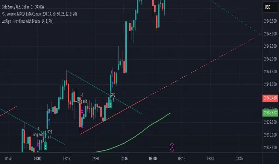
RSI+ Crypto Smart Strategy by Ignotus ### **RSI+ Crypto Smart Strategy by Ignotus**
**Description:**
The **RSI+ Crypto Smart Strategy by Ignotus** is an advanced and visually enhanced version of the classic **Relative Strength Index (RSI)**, developed by the **Crypto Smart** community. This indicator is designed to provide traders with a clear and actionable view of market momentum, overbought/oversold conditions, and potential reversal points. With its sleek design, customizable settings, and intuitive visual signals, this tool is perfect for traders who want to align their strategies with the principles of the **Crypto Smart** methodology.
Whether you're a beginner or an experienced trader, this indicator simplifies technical analysis while offering powerful insights into market behavior. It combines traditional RSI calculations with advanced visual enhancements and natural language interpretations, making it easier than ever to interpret market conditions at a glance.
---
### **Key Features:**
1. **Enhanced RSI Visualization:**
- The RSI line dynamically changes color based on its position relative to the 50-level midpoint:
- **Green** for bullish momentum (RSI > 50).
- **Red** for bearish momentum (RSI < 50).
- Overbought (default: 70) and oversold (default: 30) levels are clearly marked with customizable colors and shaded clouds for better visibility.
2. **Customizable Settings:**
- Adjust the RSI period, overbought/oversold thresholds, and background transparency to match your trading style.
- Fine-tune pivot lookback ranges and other parameters to adapt the indicator to different timeframes and assets.
3. **Interactive Information Table:**
- A compact, easy-to-read table provides real-time data on the current RSI value, its direction (▲, ▼, →), and a natural language interpretation of market conditions.
- Choose from three text sizes (small, medium, large) to optimize readability.
4. **Natural Language Interpretations:**
- The indicator includes a detailed explanation of the RSI's current state in plain English:
- Momentum trends (bullish, bearish, or neutral).
- Overbought/oversold warnings with potential reversal alerts.
- Clear guidance on whether the market is trending or ranging.
5. **Visual Buy/Sell Signals:**
- Triangles (▲ for buy, ▼ for sell) highlight potential entry and exit points based on RSI crossovers and divergence patterns.
- Configurable alerts notify you in real-time when key signals are triggered.
6. **Improved Aesthetics:**
- Clean, modern design with customizable colors for lines, clouds, and backgrounds.
- Dynamic shading and transparency options enhance chart clarity without cluttering the workspace.
---
### **How to Use This Indicator:**
- **Overbought/Oversold Zones:** Use the RSI's overbought (above 70) and oversold (below 30) zones to identify potential reversal points. Look for confirmation from price action or other indicators before entering trades.
- **Momentum Analysis:** Monitor the RSI's position relative to the 50-level midpoint to gauge bullish or bearish momentum.
- **Trend Identification:** Combine the RSI's readings with price trends to confirm the strength and direction of the market.
- **Entry/Exit Signals:** Use the visual signals (triangles) to spot potential entry and exit points. These signals are particularly useful for swing traders and scalpers.
---
### **Why Choose RSI+ Crypto Smart Strategy?**
This indicator is more than just an RSI—it's a complete tool designed to streamline your trading process. By focusing on clarity, customization, and actionable insights, the **RSI+ Crypto Smart Strategy** empowers traders to make informed decisions quickly and confidently. Whether you're trading cryptocurrencies, stocks, or forex, this indicator adapts seamlessly to your needs.
---
### **Developed by Crypto Smart:**
The **RSI+ Crypto Smart Strategy by Ignotus** is part of the **Crypto Smart** ecosystem, a community-driven initiative aimed at providing innovative tools and strategies for traders worldwide. Our mission is to simplify technical analysis while maintaining the depth and precision required for successful trading.
If you find this indicator helpful, please leave a review and share it with fellow traders! Your feedback helps us continue developing cutting-edge tools for the trading community.
---
### **Disclaimer:**
This indicator is a technical analysis tool and should not be considered financial advice. Trading involves risk, and past performance is not indicative of future results. Always conduct your own research and consult with a financial advisor before making trading decisions. Use of this indicator is at your own risk.