JK Scalp - Nishith RajwarJK Scalp Nishith Rajwar
Multi-Stochastic Rotation & Momentum Scalping Framework
JK Scalp is a rule-based momentum and rotation oscillator designed for short-term scalping and intraday execution.
It focuses on how momentum rotates across multiple stochastic speeds, instead of relying on a single oscillator or lagging averages.
This is an execution aid, not a predictive indicator.
🧠 Concept & Originality
Unlike standard stochastic tools, JK Scalp uses four synchronized stochastic layers:
• Fast (9,3) → execution timing
• Medium (14,3) → structure confirmation
• Slow (44,3) → swing context
• Trend (60,10,10) → dominant momentum regime
The core idea is quad-rotation:
High-probability trades occur when all momentum layers rotate together after reaching an extreme.
This script combines:
• Momentum rotation
• Divergence logic
• Flag continuation logic
• Trend-state filtering
into a single cohesive framework, not a simple indicator mashup.
📊 How to Use (Step-by-Step)
1️⃣ Best Timeframes
• Scalping: 1m – 3m
• Intraday: 5m – 15m
• Avoid higher timeframes (not designed for swing holding)
Works best on:
• Index options
• Index futures
• Highly liquid stocks
• Crypto majors
2️⃣ Understanding the Signals
🔁 Quad Rotation (Core Signal)
A valid rotation requires:
• Fast, Medium, Slow, and Trend stochastic moving in the same direction
• Momentum exiting Overbought / Oversold zones
• Trend stochastic supporting the move
This filters out random oscillator noise.
3️⃣ Entry Conditions
🟢 LONG Setup
• Bullish quad rotation
• Either:
– Bullish divergence OR
– Bullish flag pullback
• Fast stochastic turning up
🔴 SHORT Setup
• Bearish quad rotation
• Either:
– Bearish divergence OR
– Bearish flag pullback
• Fast stochastic turning down
⚠️ Signals are confirmation-based, not anticipatory.
4️⃣ SUPER LONG / SUPER SHORT
These appear only when:
• Quad rotation
• Divergence confirmation
They represent high-confidence momentum inflection zones, not guaranteed reversals.
5️⃣ Stop-Loss Visualization
Optional SL zones are plotted using:
• Recent swing high / low
• ATR-based buffer (configurable)
This helps traders visualize risk, not automate exits.
🎨 Visual System (Why It Looks Different)
• Multi-layer glow effects → momentum strength
• Dynamic cloud → fast vs trend dominance
• Color-shifting fast line → acceleration vs decay
• Chart overlays → execution clarity without clutter
Everything is designed for speed and readability during live trading.
⭐ Unique Selling Points (USP)
✅ Multi-speed stochastic rotation (not single-line signals)
✅ Context-first, not signal spam
✅ Built-in divergence + continuation logic
✅ Non-repainting logic
✅ Designed for scalpers, not hindsight analysis
✅ Works across indices, options, crypto, and futures
⚠️ Important Notes
• Not a standalone trading system
• Best combined with:
– Market structure
– Key levels
– Session timing
• Avoid low-liquidity or news-spike candles
This indicator guides execution, it does not replace discretion.
👤 Who This Is For
• Scalpers & intraday traders
• Options traders needing precise timing
• Traders who understand momentum & structure
• Users who want fewer but higher-quality signals
🏁 Summary
JK Scalp helps you trade momentum rotation, not overbought/oversold myths.
Wait for alignment. Execute with discipline.
Cari dalam skrip untuk "wave"

ten2 Cipher v.1Created and built by ten2crypto
This is not just another "Market Cipher" clone. This is my personal, ground-up build of a comprehensive momentum and divergence toolkit, designed to provide a deeper, more nuanced view of the market. The ten2 Cipher Divergence Engine combines the best aspects of classic momentum oscillators with a powerful, multi-layered divergence system.
This indicator was built for my own trading and is now being shared with the community.
Scalping m15 indicator RovTradingScalping Indicator Combining UT Bot and Linear Regression Candles.
UT Bot uses ATR Trailing Stop to identify entry points.
Linear Regression Candles smooth price action and provide trend signals.
The indicator is suitable for scalping trading on the M15 timeframe.

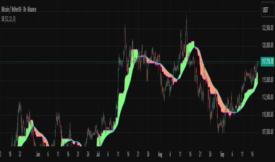
Smoothed Basis Overview and Purpose
The script calculates a smoothed mid-range basis between the highest and lowest prices over a specified period, then applies a smoothing function (smoothed moving average) to show the trend direction or momentum in a less noisy way. The area between the basis and its smoothed value is color-filled to visually highlight when the basis is above or below the smoothed average, signaling potentially bullish or bearish momentum.
Indicator Setup
length = Period length for calculating the highest and lowest values.
signal = Smoothing period used to smooth the basis.
offset =Optional horizontal shift to the plots (default 0).
Core Calculations
lower = Finds the lowest low over the past length bars.
upper = Finds the highest high over the past length bars.
basis = Calculates the midpoint between the highest and lowest.
Smoothing Calculation (Smoothed Moving Average - SMMA)
Declares smma as 0.0 initially. If the previous smma value is not available (like on the first bar), initializes with a simple moving average of basis over signal bars. Else applies formula
which gives a smoother version of basis which reacts less to sudden changes.
Plotting and Color Fill
Plots the raw basis line and smoothed basis line .
Fills the area between the basis and smoothed basis lines:
Greenish fill if the basis is above the smoothed value (potentially bullish).
Reddish fill if the basis is below the smoothed value (potentially bearish).
Interpretation and Use
The indicator visually shows where price ranges are shifting by tracking the midpoint between recent highs and lows.
The smoothed basis serves as a trend or momentum filter by dampening noise in the basis line.
When the basis is above the smoothed line (green fill), it signals upward momentum or strength; below it (red fill) suggests downward momentum or weakness.
The length and signal parameters allow tuning for different timeframes or asset volatility.
In summary, this code creates a custom smoothed oscillator based on the midpoint range of price extremes, highlighting trend changes via color fills and smoothening price action noise with an SMMA.
Adaptive Gap Bands - DolphinTradeBot1️⃣ Overview
Adaptive Gap Bands is a momentum indicator that measures the percentage difference between fast and slow moving averages. This helps identify potential overbought or oversold zones.
The goal is to analyze “gap” behaviors within a trend and generate clearer entry–exit signals.
Since the bands are anchored to the slow moving average, they are more sensitive to the trend direction, making signals stronger in line with the prevailing trend.
📌 Signals do not repaint — once confirmed, they remain fixed on the chart.
2️⃣ How It Works ?
The indicator tracks the distance between fast and slow MAs.
The indicator measures the percentage gap between the fast and slow moving averages, relative to the slow MA.
Each time the gap reaches a new extreme during a swing, that value is stored.
When the averages cross, the stored values from the last N swings (defined by Swing Count) are collected.
These gap values are then averaged to create a smoother and more adaptive reference.
The bands are built by multiplying this average gap with the % Multiplier and projecting it around the slow MA.
3️⃣ How to Use It ?
Add the script to your chart.
Green label → potential Long signal.
Red label → potential Short signal.
Signals often appear when price moves outside the adaptive bands, showing extreme momentum.
Can also be used as a reference tool in manual trades to set profit/loss expectations.
By comparing upward vs. downward gaps, it can help analyze and confirm the dominant trend direction.
4️⃣⚙️ Settings
Swing Count → Number of past swings considered.
% Multiplier → Adjusts band width (narrower or wider).
MA Lengths & Types → Choose fast and slow moving averages (EMA, SMA, RMA, etc.).

Pre-Market & Previous Day Levels 300here is the indicator pre market high low and prev day hihg low levels

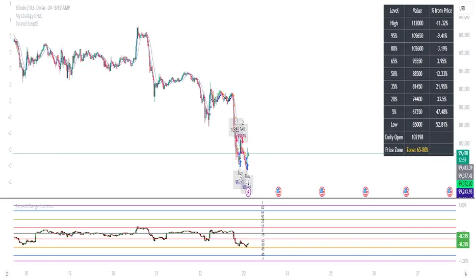
Percent Change IndicatorPercent Change Indicator Description
Overview:
The Percent Change Indicator is a Pine Script (version 6) indicator designed for TradingView to calculate and visualize the percentage change of the current close price relative to a user-selected reference price. It provides a customizable interface to display percentage changes as candlesticks or a line plot, with optional horizontal lines and labels for key levels. The indicator also includes visual signals and alerts for user-defined percentage thresholds, making it useful for identifying significant price movements.
Key Features:
1. Percentage Change Calculation:
- Computes the percentage change of the current close price compared to a reference price, scaled by a user-defined length parameter.
- Formula: percentChange = (close - refPrice) / refPrice * len
- The reference price is sourced from a user-selected timeframe (default: 1D) and price type (Open, High, Low, Close, HL2, HLC3, or HLCC4).
2. Visualization Options:
- Candlestick Plot: Displays percentage change as candlesticks, colored green for rising values and red for falling values.
- Line Plot: Plots the percentage change as a line, with the same color logic.
- Horizontal Lines: Optional horizontal lines at key percentage levels (0%, ±0.2%, ±0.5%, ±0.8%, ±1%) for reference.
- Labels: Optional labels for percentage levels (0, ±15%, ±35%, ±50%, ±65%, ±85%, ±100%) displayed at the chart's right edge.
- All visualizations are toggleable via input settings.
3. Signal and Alert System:
- Threshold-Based Signals: Plots green triangles below bars for long signals (percent change above a user-defined threshold) and red triangles above bars for short signals (percent change below the threshold).
- Alerts: Configurable alerts for long and short conditions, triggered when the percentage change crosses the user-defined threshold (default: 2%). Alert messages include the threshold value for clarity.
4. Customizable Inputs:
- Show Labels: Toggle visibility of percentage level labels (default: true).
- Show Percentage Change: Toggle the line plot of percentage change (default: true).
- Show HLines: Toggle visibility of horizontal reference lines (default: false).
- Show Candle Plot: Toggle the candlestick plot (default: true).
- Percent Change Length: Adjust the scaling factor for percentage change (default: 14).
- Plot Timeframe: Select the timeframe for the reference price (default: 1D).
- Price Type: Choose the reference price type (Open, High, Low, Close, HL2, HLC3, HLCC4; default: Open).
- Percentage Threshold: Set the threshold for long/short signals and alerts (default: 0.02 or 2%).
How It Works:
- The indicator fetches the reference price using request.security() based on the selected timeframe and price type.
- It calculates the percentage change and scales it by the user-defined length.
- Visuals (candlesticks, lines, labels, horizontal lines) are plotted based on user preferences.
- Long and short signals are generated when the percentage change exceeds or falls below the user-defined threshold, with corresponding triangles plotted and alerts triggered.
Use Cases:
- Trend Identification: Monitor significant price movements relative to a reference price.
- Signal Generation: Identify potential entry/exit points based on percentage change thresholds.
- Custom Analysis: Analyze price changes across different timeframes and price types for various trading strategies.
- Alert Notifications: Receive alerts for significant price movements to stay informed without constant chart monitoring.
Setup Instructions:
1. Add the indicator to a TradingView chart.
2. Adjust input settings (timeframe, price type, threshold, etc.) to suit your analysis.
3. Enable/disable visualization options (candlesticks, lines, labels, horizontal lines) as needed.
4. Set up alerts in TradingView:
- Go to the "Alerts" tab and select "Percent Change Indicator."
- Choose "Long Alert" or "Short Alert" to monitor threshold crossings.
- Configure alert frequency and notification method (e.g., email, webhook).
Notes:
- The indicator is non-overlay, displayed in a separate pane below the main chart.
- Alerts trigger on bar close by default; adjust TradingView alert settings for real-time notifications if needed.
- The indicator is released under the Mozilla Public License 2.0.
Author: Dshergill
This indicator is ideal for traders seeking a flexible tool to track percentage-based price movements with customizable visuals and alerts.
NY ORB + Fakeout Detector🗽 NY ORB + Fakeout Detector
This indicator automatically plots the New York Opening Range (ORB) based on the first 15 minutes of the NY session (15:30–15:45 CEST / 13:30–13:45 UTC) and detects potential fakeouts (false breakouts).
🔍 Key Features:
✅ Plots ORB high and low based on the 15-minute NY open range
✅ Automatically detects fake breakouts (price wicks beyond the box but closes back inside)
✅ Visual markers:
🔺 "Fake ↑" if a fake breakout occurs above the range
🔻 "Fake ↓" if a fake breakout occurs below the range
✅ Gray background highlights the ORB session window
✅ Designed for scalping and short-term breakout strategies
🧠 Best For:
Intraday traders looking for NY volatility setups
Scalpers using ORB-based entries
Traders seeking early-session fakeout traps to avoid false signals
Those combining with EMA 12/21, volume, or other confluence tools

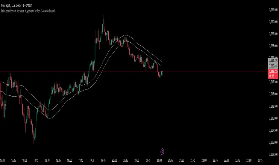
Price equilibrium between buyers and sellers [Soroush Rezaei]This indicator visualizes the dynamic balance between buyers and sellers using two simple moving averages (SMAs) based on the high and low prices.
The green line (SMA of highs) reflects the upper pressure zone, while the red line (SMA of lows) represents the lower support zone.
When price hovers between these two levels, it often signals a state of temporary equilibrium — a consolidation zone where buyers and sellers are relatively balanced.
Use this tool to:
Identify ranging or balanced market phases
Spot potential breakout or reversal zones
Enhance your multi-timeframe or price action strategy
Recommended for intraday and swing traders seeking visual clarity on market structure and momentum zones.
Solar VPR (No EVMA) + Alpha TrendThis Pine Script v6 indicator combines Solar VPR (without EVMA slow average) and Alpha Trend to identify potential trading opportunities.
Solar VPR calculates a Simple Moving Average (SMA) of the hlc3 price and defines upper/lower bands based on a percentage multiplier. It highlights bullish (green) and bearish (red) zones.
Alpha Trend applies ATR-based smoothing to an SMA, identifying trend direction. Blue indicates an uptrend, while orange signals a downtrend.
Buy/Sell Signals appear when price crosses Alpha Trend and aligns with Solar VPR direction.

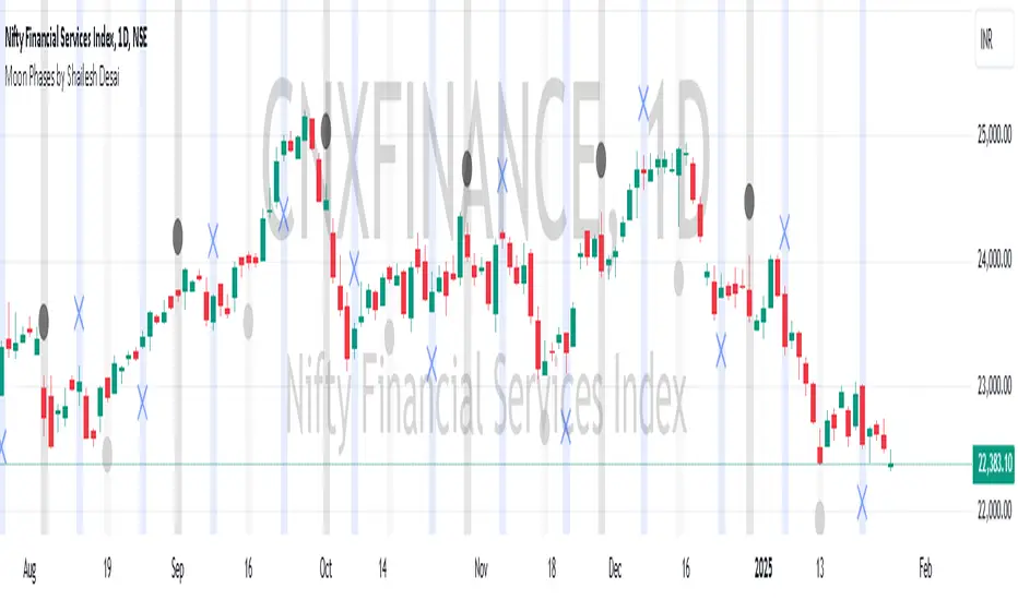
Moon Phases by Shailesh DesaiTrading Strategy Based on Lunar Phases
This custom trading indicator leverages the power of lunar cycles to provide unique market insights based on the four primary moon phases: New Moon, First Quarter, Full Moon, and Third Quarter. By aligning your trades with the natural rhythm of the moon, this strategy offers a different perspective to trading and can help enhance decision-making based on the cyclical nature of the market.
Key Features:
1. Moon Phase Identification:
o The indicator automatically identifies the current moon phase based on the user's selected timeframe and marks it on the chart.
o Each phase is visualized with a specific symbol and color to help traders easily recognize the current moon phase:
New Moon/Waxing Moon: Represented by a circle (colored as per user input).
First Quarter: Represented by a cross (colored as per user input).
Full Moon/Waning Moon: Represented by a circle (colored as per user input).
Third Quarter: Represented by a cross (colored as per user input).
2. Automatic Moon Phase Transition Detection:
o The indicator tracks and highlights when a phase change occurs. This feature ensures you are always aware of when the market moves from one phase to another.
o Moon phase changes are only visualized on the first bar of each new phase to avoid cluttering the chart.
3. Background Color Indicators:
o The background color dynamically changes according to the current moon phase, helping to reinforce the phase context for the trader. This feature makes it easy to see at a glance which phase the market is in.
4. Customizable Appearance:
o Customize the color of each moon phase to suit your preferences. Adjust the colors for the New Moon, First Quarter, Full Moon, and Third Quarter to align with your visual strategy.
5. Avoids Unsupported Timeframes:
o This indicator does not support monthly timeframes, ensuring that it operates smoothly only on timeframes that are compatible with the lunar cycle.
How to Use:
• The moon phases are thought to have an influence on human behavior and the market's psychology, making this indicator useful for traders who wish to integrate lunar cycles into their strategy.
• Traders can use the phase changes as an indicator of potential market momentum or reversal points. For example:
o New Moon may indicate the beginning of a new cycle, signaling a potential upward or downward move.
o Full Moon might suggest a peak or significant shift in market direction.
o First Quarter and Third Quarter phases may represent moments of consolidation or decision points.
Ideal for:
• Traders interested in cycle-based strategies or looking to experiment with new approaches.
• Those who believe in the influence of natural forces, including moon phases, on market movements.
• Technical analysts who want to add another layer of insights to their chart analysis.
Important Notes:
• The indicator uses precise astronomical calculations to identify the correct phase, ensuring accuracy.
• It’s important to understand that moon phase-based trading is not a standalone strategy but should ideally be combined with other technical analysis tools for maximum effectiveness.
STRATEGY Fibonacci Levels with High/Low Criteria - AYNET
Here is an explanation of the Fibonacci Levels Strategy with High/Low Criteria script:
Overview
This strategy combines Fibonacci retracement levels with high/low criteria to generate buy and sell signals based on price crossing specific thresholds. It utilizes higher timeframe (HTF) candlesticks and user-defined lookback periods for high/low levels.
Key Features
Higher Timeframe Integration:
The script calculates the open, high, low, and close values of the higher timeframe (HTF) candlestick.
Users can choose to calculate levels based on the current or the last HTF candle.
Fibonacci Levels:
Fibonacci retracement levels are dynamically calculated based on the HTF candlestick's range (high - low).
Users can customize the levels (0.000, 0.236, 0.382, 0.500, 0.618, 0.786, 1.000).
High/Low Lookback Criteria:
The script evaluates the highest high and lowest low over user-defined lookback periods.
These levels are plotted on the chart for visual reference.
Trade Signals:
Long Signal: Triggered when the close price crosses above both:
The lowest price criteria (lookback period).
The Fibonacci level 3 (default: 0.5).
Short Signal: Triggered when the close price crosses below both:
The highest price criteria (lookback period).
The Fibonacci level 3 (default: 0.5).
Visualization:
Plots Fibonacci levels and high/low criteria on the chart for easy interpretation.
Inputs
Higher Timeframe:
Users can select the timeframe (default: Daily) for the HTF candlestick.
Option to calculate based on the current or last HTF candle.
Lookback Periods:
lowestLookback: Number of bars for the lowest low calculation (default: 20).
highestLookback: Number of bars for the highest high calculation (default: 10).
Fibonacci Levels:
Fully customizable Fibonacci levels ranging from 0.000 to 1.000.
Visualization
Fibonacci Levels:
Plots six customizable Fibonacci levels with distinct colors and transparency.
High/Low Criteria:
Plots the highest and lowest levels based on the lookback periods as reference lines.
Trading Logic
Long Condition:
Price must close above:
The lowest price criteria (lowcriteria).
The Fibonacci level 3 (50% retracement).
Short Condition:
Price must close below:
The highest price criteria (highcriteria).
The Fibonacci level 3 (50% retracement).
Use Case
Trend Reversal Strategy:
Combines Fibonacci retracement with recent high/low criteria to identify potential reversal or breakout points.
Custom Timeframe Analysis:
Incorporates higher timeframe data for multi-timeframe trading strategies.

Gradient Filter with Fibonacci-AYNETExplanation of the Combined Features:
Dynamic Gradient Filter:
This section remains as in the previous example, calculating a smoothed filter (filt) with dynamic gradient coloring.
The color of the filter line transitions from red to green based on its RSI value.
Fibonacci Levels:
Calculates key Fibonacci retracement levels (0.0, 0.236, 0.382, 0.5, 0.618, and 1.0) over a user-defined lookback period (fib_length).
Uses the highest high and lowest low in the lookback period to determine the range.
Plotting Fibonacci Levels:
Each Fibonacci level is drawn as a horizontal line.
The lines extend back by the lookback period and are styled with dotted lines for clarity.
Features:
Customizable Inputs:
Users can enable or disable Fibonacci levels (show_fib_levels).
Adjust the color (fib_color) and width (fib_width) of Fibonacci lines.
Integrated Dynamic Filter:
Combines the filtered line with Fibonacci retracement levels to provide multi-dimensional insights.
Use Case:
Dynamic Filter:
Observe how the filtered line behaves near Fibonacci levels for potential trend continuations or reversals.
Fibonacci Levels:
Use retracement levels as key support/resistance zones to make trading decisions.
This combined script is now more functional, blending the dynamic gradient filter with Fibonacci retracement levels. Test this script in different market conditions, and let me know if additional features are required! 😊

ICT Setup 03 [TradingFinder] Judas Swing NY 9:30am + CHoCH/FVG🔵 Introduction
Judas Swing is an advanced trading setup designed to identify false price movements early in the trading day. This advanced trading strategy operates on the principle that major market players, or "smart money," drive price in a certain direction during the early hours to mislead smaller traders.
This deceptive movement attracts liquidity at specific levels, allowing larger players to execute primary trades in the opposite direction, ultimately causing the price to return to its true path.
The Judas Swing setup functions within two primary time frames, tailored separately for Forex and Stock markets. In the Forex market, the setup uses the 8:15 to 8:30 AM window to identify the high and low points, followed by the 8:30 to 8:45 AM frame to execute the Judas move and identify the CISD Level break, where Order Block and Fair Value Gap (FVG) zones are subsequently detected.
In the Stock market, these time frames shift to 9:15 to 9:30 AM for identifying highs and lows and 9:30 to 9:45 AM for executing the Judas move and CISD Level break.
Concepts such as Order Block and Fair Value Gap (FVG) are crucial in this setup. An Order Block represents a chart region with a high volume of buy or sell orders placed by major financial institutions, marking significant levels where price reacts.
Fair Value Gap (FVG) refers to areas where price has moved rapidly without balance between supply and demand, highlighting zones of potential price action and future liquidity.
Bullish Setup :
Bearish Setup :
🔵 How to Use
The Judas Swing setup enables traders to pinpoint entry and exit points by utilizing Order Block and FVG concepts, helping them align with liquidity-driven moves orchestrated by smart money. This setup applies two distinct time frames for Forex and Stocks to capture early deceptive movements, offering traders optimized entry or exit moments.
🟣 Bullish Setup
In the Bullish Judas Swing setup, the first step is to identify High and Low points within the initial time frame. These levels serve as key points where price may react, forming the basis for analyzing the setup and assisting traders in anticipating future market shifts.
In the second time frame, a critical stage of the bullish setup begins. During this phase, the price may create a false break or Fake Break below the low level, a deceptive move by major players to absorb liquidity. This false move often causes smaller traders to enter positions incorrectly. After this fake-out, the price reverses upward, breaking the CISD Level, a critical point in the market structure, signaling a potential bullish trend.
Upon breaking the CISD Level and reversing upward, the indicator identifies both the Order Block and Fair Value Gap (FVG). The Order Block is an area where major players typically place large buy orders, signaling potential price support. Meanwhile, the FVG marks a region of supply-demand imbalance, signaling areas where price might react.
Ultimately, after these key zones are identified, a trader may open a buy position if the price reaches one of these critical areas—Order Block or FVG—and reacts positively. Trading at these levels enhances the chance of success due to liquidity absorption and support from smart money, marking an opportune time for entering a long position.
🟣 Bearish Setup
In the Bearish Judas Swing setup, analysis begins with marking the High and Low levels in the initial time frame. These levels serve as key zones where price could react, helping to signal possible trend reversals. Identifying these levels is essential for locating significant bearish zones and positioning traders to capitalize on downward movements.
In the second time frame, the primary bearish setup unfolds. During this stage, price may exhibit a Fake Break above the high, causing a brief move upward and misleading smaller traders into incorrect positions. After this false move, the price typically returns downward, breaking the CISD Level—a crucial bearish trend indicator.
With the CISD Level broken and a bearish trend confirmed, the indicator identifies the Order Block and Fair Value Gap (FVG). The Bearish Order Block is a region where smart money places significant sell orders, prompting a negative price reaction. The FVG denotes an area of supply-demand imbalance, signifying potential selling pressure.
When the price reaches one of these critical areas—the Bearish Order Block or FVG—and reacts downward, a trader may initiate a sell position. Entering trades at these levels, due to increased selling pressure and liquidity absorption, offers traders an advantage in profiting from price declines.
🔵 Settings
Market : The indicator allows users to choose between Forex and Stocks, automatically adjusting the time frames for the "Opening Range" and "Trading Permit" accordingly: Forex: 8:15–8:30 AM for identifying High and Low points, and 8:30–8:45 AM for capturing the Judas move and CISD Level break. Stocks: 9:15–9:30 AM for identifying High and Low points, and 9:30–9:45 AM for executing the Judas move and CISD Level break.
Refine Order Block : Enables finer adjustments to Order Block levels for more accurate price responses.
Mitigation Level OB : Allows users to set specific reaction points within an Order Block, including: Proximal: Closest level to the current price. 50% OB: Midpoint of the Order Block. Distal: Farthest level from the current price.
FVG Filter : The Judas Swing indicator includes a filter for Fair Value Gap (FVG), allowing different filtering based on FVG width: FVG Filter Type: Can be set to "Very Aggressive," "Aggressive," "Defensive," or "Very Defensive." Higher defensiveness narrows the FVG width, focusing on narrower gaps.
Mitigation Level FVG : Like the Order Block, you can set price reaction levels for FVG with options such as Proximal, 50% OB, and Distal.
CISD : The Bar Back Check option enables traders to specify the number of past candles checked for identifying the CISD Level, enhancing CISD Level accuracy on the chart.
🔵 Conclusion
The Judas Swing indicator helps traders spot reliable trading opportunities by detecting false price movements and key levels such as Order Block and FVG. With a focus on early market movements, this tool allows traders to align with major market participants, selecting entry and exit points with greater precision, thereby reducing trading risks.
Its extensive customization options enable adjustments for various market types and trading conditions, giving traders the flexibility to optimize their strategies. Based on ICT techniques and liquidity analysis, this indicator can be highly effective for those seeking precision in their entry points.
Overall, Judas Swing empowers traders to capitalize on significant market movements by leveraging price volatility. Offering precise and dependable signals, this tool presents an excellent opportunity for enhancing trading accuracy and improving performance

Fair Value Gaps Setup 01 [TradingFinder] FVG Absorption + CHoCH🔵 Introduction
🟣 Market Structures
Market structures exhibit a fractal and nested nature, which leads us to classify them into internal (minor) and external (major) categories. Definitions of market structure vary, with different methodologies such as Smart Money and ICT offering distinct interpretations.
To identify market structure, the initial step involves examining key highs and lows. An uptrend is characterized by successive highs and lows that are higher than their predecessors. Conversely, a downtrend is marked by successive lows and highs that are lower than their previous counterparts.
🟣 Market Trends and Movements
Market trends consist of two primary types of movements :
Impulsive Movements : These movements align with the main trend and are characterized by high strength and momentum.
Corrective Movements : These movements counter the main trend and are marked by lower strength and momentum.
🟣 Break of Structure (BOS)
In a downtrend, a Break of Structure (BOS) occurs when the price falls below the previous low and establishes a new low (LL). In an uptrend, a BOS, also known as a Market Structure Break (MSB), happens when the price rises above the last high.
To confirm a trend, at least one BOS is necessary, which requires the price to close at least one candle beyond the previous high or low.
🟣 Change of Character (CHOCH)
Change of Character (CHOCH) is a crucial concept in market structure analysis, indicating a shift in trend. A trend concludes with a CHOCH, also referred to as a Market Structure Shift (MSS).
For example, in a downtrend, the price continues to drop with BOS, showcasing the trend's strength. However, when the price rises and exceeds the last high, a CHOCH occurs, signaling a potential transition from a downtrend to an uptrend.
It is essential to note that a CHOCH does not immediately indicate a buy trade. Instead, it is prudent to wait for a BOS in the upward direction to confirm the uptrend. Unlike BOS, a CHOCH confirmation does not require a candle to close; merely breaking the previous high or low with the candle's wick is sufficient.
🟣 Spike | Inefficiency | Imbalance
All these terms mean fast price movement in the shortest possible time.
🟣 Fair Value Gap (FVG)
To pinpoint the "Fair Value Gap" (FVG) on a chart, a detailed candle-by-candle analysis is necessary. This process involves focusing on candles with substantial bodies and evaluating them in relation to the candles immediately before and after them.
Here are the steps :
Identify the Central Candle : Look for a candle with a large body.
Examine Adjacent Candles : The candles before and after this central candle should have long shadows, and their bodies must not overlap with the body of the central candle.
Determine the FVG Range : The distance between the shadows of the first and third candles defines the FVG range.
This method helps in accurately identifying the Fair Value Gap, which is crucial for understanding market inefficiencies and potential price movements.
🟣 Setup
This setup is based on Market Structure and FVG. After a change of character and the formation of FVG in the last lag of the price movement, we are looking for trading positions in the price pullback.
Bullish Setup :
Bearish Setup :
🔵 How to Use
After forming the setup, you can enter the trade using a pending order or after receiving confirmation. To increase the probability of success, you can adjust the pivot period market structure settings or modify the market movement coefficient in the formation leg of the FVG.
Bullish Setup :
Bearish Setup :
🔵 Setting
Pivot Period of Market Structure Detector :
This parameter allows you to configure the zigzag period based on pivots. Adjusting this helps in accurately detecting order blocks.
Show major Bullish ChoCh Lines :
You can toggle the visibility of the Demand Main Zone and "ChoCh" Origin, and customize their color as needed.
Show major Bearish ChoCh Lines :
Similar to the Demand Main Zone, you can control the visibility and color of the Supply Main Zone and "ChoCh" Origin.
FVG Detector Multiplier Factor :
This feature lets you adjust the size of the moves forming the Fair Value Gaps (FVGs) using the Average True Range (ATR). The default value is 1, suitable for identifying most setups. Adjust this value based on the specific symbol and market for optimal results.
FVG Validity Period :
This parameter defines the validity period of an FVG in terms of the number of candles. By default, an FVG remains valid for up to 15 candles, but you can adjust this period as needed.
Mitigation Level FVG :
This setting establishes the basic level of an FVG. When the price reaches this level, the FVG is considered mitigated.
Level in Low-Risk Zone :
This feature aims to reduce risk by dividing the FVG into two equal areas: "Premium" (upper area) and "Discount" (lower area). For lower risk, ensure that "Demand FVG" is in the "Discount" area and "Supply FVG" in the "Premium" area. This feature is off by default.
Show or Hide :
Given the potential abundance of setups, displaying all on the chart can be overwhelming. By default, only the last setup is shown, but you can enable the option to view all setups.
Alert Settings :
On / Off : Toggle alerts on or off.
Message Frequency : Determine how often alerts are triggered.
Options include :
"All" (alerts every time the function is called)
"Once Per Bar" (alerts only on the first call within the bar)
"Once Per Bar Close" (alerts only at the last script execution of the real-time bar upon closing)
The default setting is "Once Per Bar".
Show Alert Time by Time Zone : Set the alert time based on your preferred time zone, such as "UTC-4" for New York time. The default is "UTC".
Display More Info : Optionally show additional details like the price range of the order blocks and the date, hour, and minute in the alert message. Set this to "Off" if you prefer not to receive this information.

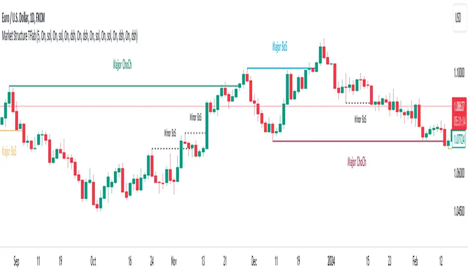
Market Structures SMC [TradingFinder] BOS/CHoCH Major & Minor🟣Introduction
Understanding market structure involves analyzing market behavior. In other words, market structure encompasses how the market forms and evolves within trends.
Market structures are typically fractal and nested, so we categorize them into internal (minor) and external (major) structures. There are various definitions of market structure, with different approaches such as Smart Money and ICT providing their own interpretations.
🟣How to Use
The first step in identifying market structure is to analyze key highs and lows. An uptrend is formed when highs and lows are successively higher than previous ones. Similarly, in a downtrend, lows and highs are successively lower than previous ones.
Market trends consist of two types of movements :
•Impulsive movements
•Corrective movements
Impulsive movements align with the main trend and possess high strength and momentum. Conversely, corrective movements go against the main trend and have lower strength and momentum. The following example illustrates these concepts.
🔵 Identifying Break of Structure (BOS)
In a specific trend, for example in a downtrend, when the price breaks below the previous low and forms a new low (LL), a Break of Structure occurs. In an uptrend, a BOS (Market Structure Break or MSB) happens when the price rises and surpasses the last high.
We need at least one BOS to confirm a trend. Breaking above or below the previous high or low must be confirmed by closing at least one candle after that level.
🔵 Identifying Change of Character (CHOCH)
Change of Character (CHOCH) is a key concept in market structure analysis. A change in structure signals a trend change. In other words, a trend ends with a CHOCH (Market Structure Shift or MSS). For instance, in a downtrend, the price declines with BOS.
BOS indicates the strength of the trend, but when the price increases and surpasses the last high, a CHOCH occurs, signaling a shift from a downtrend to an uptrend.
This does not mean entering a buy trade; instead, we should wait for a BOS in the upward direction to confirm the uptrend. Unlike BOS, confirming a CHOCH does not require a candle to close; simply breaking above or below the previous high or low with the candle's wick is sufficient. The following examples show bearish and bullish CHOCH.
🔵 Range Market Structure
Besides uptrends and downtrends, a third structure often found in the market is the range or sideways structure. In this state, the power of buyers and sellers is almost equal, and the market lacks a clear trend.
Many traders believe that the Forex market ranges 80% of the time. Therefore, it requires a lot of patience to wait for a new trend to start.
🟣 Settings
Through the settings, you can customize the display, visibility, and color of each line as desired.
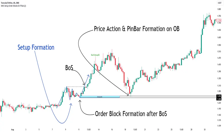
Smart Money Setup 06 [TradingFinder] Liquidity Sweeps + OB Swing🔵 Introduction
Smart Money, managed by large investors, injects significant capital into financial markets by entering real capital markets.
Capital entering the market by this group of individuals is called smart money. Traders can profit from financial markets by following such individuals.
Therefore, smart money can be considered one of the effective methods for analyzing financial markets.
Sometimes, before a market movement, fluctuation movements that create price movement cause many traders' "Stop Loss" to be triggered. These movements are created in various patterns.
One of these patterns is similar to an "Expanding Triangle", which touches the stop loss of individuals who have placed their stop loss in the cash area in the form of 5 consecutive openings.
To better understand this setup, pay attention to the images below.
Bullish Setup Details :
Bearish Setup Details :
🔵 How to Use
After adding the indicator to the chart, wait for trading opportunities to appear. By changing the "Time Frame" and "Pivot Period", you can see different trading positions.
In general, the smaller the "Time Frame" and "Pivot Period", the more likely trading opportunities will appear.
Bullish Setup Details on Chart :
Bearish Setup Details on Chart :
🔵 Settings
You have access to "Pivot Period", "Order Block Refine", and "Refine Mode" through settings.
By changing the "Pivot Period", you can change the range of zigzag that identifies the setup.
Through "Order Block Refine", you can specify whether you want to refine the width of the order blocks or not. It is set to "On" by default.
Through "Refine Mode", you can specify how to improve order blocks.
If you are "risk-averse", you should set it to "Defensive" mode because in this mode, the width of the order blocks decreases, the number of your trades decreases, and the "reward-to-risk ratio "increases.
If you are on the opposite side and are "risk-taker", you can set it to "Aggressive" mode. In this mode, the width of the order blocks increases, and the likelihood of losing positions decreases.

Smart Money Setup 03 [TradingFinder] Minor OB & Trend Proof🔵 Introduction
The "Smart Money Concept" transcends mere technical trading strategies; it embodies a comprehensive philosophy elucidating market dynamics. Central to this concept is the acknowledgment that influential market participants manipulate price actions, presenting challenges for retail traders.
As a "retail trader", aligning your strategy with the behavior of "Smart Money," primarily market makers, is paramount. Understanding their trading patterns, which revolve around supply, demand, and market structure, forms the cornerstone of your approach. Consequently, decisions to enter trades should be informed by these considerations.
🟣 Important Note
In this setup, pattern formation revolves around the robustness of the "Stop Hunt" targeting retail traders.
When this stop hunt occurs, if the price tests below the minor pivot or above the minor pivot, a "Minor Order Block" is formed.
Similarly, if the price tests below the major pivot or above the major pivot, a "Major Order Block" is formed.
Since the price hasn't successfully broken the major pivots before breaking the Top or Bottom, it can be inferred that the minor pivots formed within a leg of price movement exhibit a "Range" structure.
For a deeper comprehension of this setup, refer to the accompanying visual aids below.
Bullish Setup Details :
Bearish Setup Details :
🔵 How to Use
Upon integrating the indicator into your chart, exercise patience as you await the evolution of the trading setup.
Experiment with different trading positions by adjusting both the "Time Frame" and "Pivot Period". Typically, setups materializing over longer "Time Frames" and "Pivot Periods" carry heightened validity.
Bullish Setup Details on Chart :
Bearish Setup Details on Chart :
Within the settings, you possess the flexibility to modify the "Pivot Period" input to tailor the indicator to your preferences.
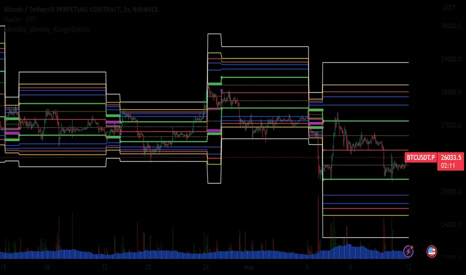
Monday_Weekly_Range/ErkOzi/Deviation Level/V1"Hello, first of all, I believe that the most important levels to look at are the weekly Fibonacci levels. I have planned an indicator that automatically calculates this. It models a range based on the weekly opening, high, and low prices, which is well-detailed and clear in my scans. I hope it will be beneficial for everyone.
***The logic of the Monday_Weekly_Range indicator is to analyze the weekly price movement based on the trading range formed on Mondays. Here are the detailed logic, calculation, strategy, and components of the indicator:
***Calculation of Monday Range:
The indicator calculates the highest (mondayHigh) and lowest (mondayLow) price levels formed on Mondays.
If the current bar corresponds to Monday, the values of the Monday range are updated. Otherwise, the values are assigned as "na" (undefined).
***Calculation of Monday Range Midpoint:
The midpoint of the Monday range (mondayMidRange) is calculated using the highest and lowest price levels of the Monday range.
***Fibonacci Levels:
// Calculate Fibonacci levels
fib272 = nextMondayHigh + 0.272 * (nextMondayHigh - nextMondayLow)
fib414 = nextMondayHigh + 0.414 * (nextMondayHigh - nextMondayLow)
fib500 = nextMondayHigh + 0.5 * (nextMondayHigh - nextMondayLow)
fib618 = nextMondayHigh + 0.618 * (nextMondayHigh - nextMondayLow)
fibNegative272 = nextMondayLow - 0.272 * (nextMondayHigh - nextMondayLow)
fibNegative414 = nextMondayLow - 0.414 * (nextMondayHigh - nextMondayLow)
fibNegative500 = nextMondayLow - 0.5 * (nextMondayHigh - nextMondayLow)
fibNegative618 = nextMondayLow - 0.618 * (nextMondayHigh - nextMondayLow)
fibNegative1 = nextMondayLow - 1 * (nextMondayHigh - nextMondayLow)
fib2 = nextMondayHigh + 1 * (nextMondayHigh - nextMondayLow)
***Fibonacci levels are calculated using the highest and lowest price levels of the Monday range.
Common Fibonacci ratios such as 0.272, 0.414, 0.50, and 0.618 represent deviation levels of the Monday range.
Additionally, the levels are completed with -1 and +1 to determine at which level the price is within the weekly swing.
***Visualization on the Chart:
The Monday range, midpoint, Fibonacci levels, and other components are displayed on the chart using appropriate shapes and colors.
The indicator provides a visual representation of the Monday range and Fibonacci levels using lines, circles, and other graphical elements.
***Strategy and Usage:
The Monday range represents the starting point of the weekly price movement. This range plays an important role in determining weekly support and resistance levels.
Fibonacci levels are used to identify potential reaction zones and trend reversals. These levels indicate where the price may encounter support or resistance.
You can use the indicator in conjunction with other technical analysis tools and indicators to conduct a more comprehensive analysis. For example, combining it with trendlines, moving averages, or oscillators can enhance the accuracy.
When making investment decisions, it is important to combine the information provided by the indicator with other analysis methods and use risk management strategies.
Thank you in advance for your likes, follows, and comments. If you have any questions, feel free to ask."
Dual Dynamic Fibonacci Retracement — Long and Short Duration
Title : "The Dual-Dynamic Fibonacci Retracement Script: An Advanced Tool for Comprehensive Market Analysis"
As the author of the "Dual-Dynamic Fibonacci Retracement Script", I am delighted to introduce you to this cutting-edge tool for technical analysis. Unlike conventional Fibonacci scripts, this advanced model incorporates multiple unique features and adjustments that make it a powerful asset for any market analyst. Whether you're dealing with forex, commodities, equities or any other market, this script is versatile enough to enhance your trading strategy.
Uniqueness & Differentiation:
The "Dual-Dynamic Fibonacci Script" stands out by offering two distinct lookback periods. This feature is what separates it from other scripts available in the market. The first lookback period is longer, focusing on capturing broader market trends. The second lookback period is shorter, allowing for a more granular analysis of near-term market fluctuations. This dual perspective provides a more comprehensive view of the market, allowing you to see both the forest and the trees at the same time.
Fibonacci Levels:
While offering the standard Fibonacci retracement levels (0.236, 0.382, 0.5, 0.618, 0.786, and 1.0), the script also gives you the ability to plot 0.114 and 0.886 levels. These additional levels offer an extra layer of depth to your analysis, and can prove crucial in high-volatility markets where they often serve as significant support and resistance points.
Customizable Line Shifts and Extends:
This script provides options for customization of the shift and extension of the plotted lines. This means you can adjust the start and end points of the Fibonacci lines according to your personal trading style and strategy. This level of personalization is not typically available in other scripts, and it allows for a more tailored visual representation.
Flexible Trading Positioning:
Depending on whether the closing price is above or below the midpoint of the pivot high and pivot low, the Fibonacci retracement levels are adjusted accordingly. This ensures the script remains relevant and useful regardless of market conditions.
Clean Visualization:
To prevent clutter and maintain focus on the most relevant price action, the script removes old Fibonacci lines and plots new ones once a new pivot high or low is identified. This clean visualization helps keep your analysis focused and sharp.
How to Use the Script:
To get started, simply adjust the lookback periods according to your trading strategy. If you're a long-term investor or prefer swing trading, a longer lookback period might be appropriate. Conversely, if you're a day trader, a shorter lookback period might be more beneficial.
The "Shift" and "Extend" inputs allow you to control the positioning of the Fibonacci lines on your chart. Positive values shift the lines to the right, while negative values shift them to the left.
You also have the choice to plot the additional Fibonacci levels (0.114 and 0.886) via the "Plot 0.114 and 0.886 levels?" input. Similarly, the "Plot second set of levels?" input lets you decide whether to display the second set of Fibonacci levels derived from the shorter lookback period.
Like any technical analysis tool, this script is most effective when used in conjunction with other indicators and methods of analysis. It is designed to work well in trending markets, where Fibonacci retracements can often indicate potential reversal levels. However, it's always recommended to use a holistic approach to market analysis to maximize the likelihood of successful trades.
Note: the two lines drawn on the chart are there to help the user identify the levels from which the two respective Fib sequences are calculated.
~~~
Input Explanations:
Long Period Pivot High/Low Lookback and Short Period Pivot High/Low Lookback : These settings determine the length of the lookback periods for the long-term and short-term pivot points, respectively. A pivot point is a technical analysis indicator used to determine the overall trend of the market over different time frames. The pivot points are then used to calculate the Fibonacci levels. A longer lookback period will identify pivot points over a broader time frame, capturing major market trends, while a shorter lookback period will identify pivot points over a narrower time frame, capturing more immediate market movements.
Long Period Fibonacci Level Shift and Short Period Fibonacci Level Shift : These inputs control the shift of the Fibonacci levels based on the long and short lookback periods, respectively. If you want to shift the Fibonacci levels to the right, increase the value. If you want to shift the Fibonacci levels to the left, decrease the value. This allows you to adjust the Fibonacci levels to better align with your analysis.
Long Period Fibonacci Level Extend and Short Period Fibonacci Level Extend : These inputs control the extension of the Fibonacci levels based on the long and short lookback periods, respectively. If you want the Fibonacci levels to extend further to the right, increase the value. If you want the Fibonacci levels to extend less to the right, decrease the value. This feature provides the flexibility to adjust the length of the Fibonacci levels according to your personal trading preferences and strategy.
Plot 0.114 and 0.886 levels? : This setting gives you the ability to plot the additional 0.114 and 0.886 Fibonacci levels. These levels provide extra depth to your analysis, particularly in highly volatile markets where they can act as significant support and resistance levels.
Plot second set of levels? : This input allows you to decide whether to plot the second set of Fibonacci levels based on the short lookback period. Displaying this second set of levels can provide a more granular view of market movements and potential reversal points, enhancing your overall analysis.

CDC Fibonacci Retracement and ExtensionThis indicator is meant to be used as a tool to quickly identify
fibonacci retracements and projections in multiple charts during
the same date range.
Users can set the calculation date range and quickly flip through
different charts for comparisons
Steps for using this indicator is as follows:
1. Specify Start Date and End Date for calculations
2. Choose Open-ended mode for just retracements, this will disregard
end date in calculations.
3. Select price source, if Use Highs/Lows is selected, the indicator will
use high and low prices for calculation, if not, closing price eill
be used instead
4. Select and/or modify retracement / projection lines as you see fit.
5. Enjoy the result!

Neowave chart cash dataScript Cash is a neo-analytic style data. Add to use on the chart and then hide the candlesticks and enjoy the cash data.
The daily data cache is set normally. To change the settings, be sure to change the D indicator to W for weekly and M for monthly.
Also enter the number of minutes to use in the hourly time frame, for example four hours (240)
...
When you change the data cache settings in the settings, you must follow the rule of one fortieth of the Neowave style and move the time frame chart to forty to analyze it, for example, for a daily time frame go to 30 minutes.
I hope it is used.