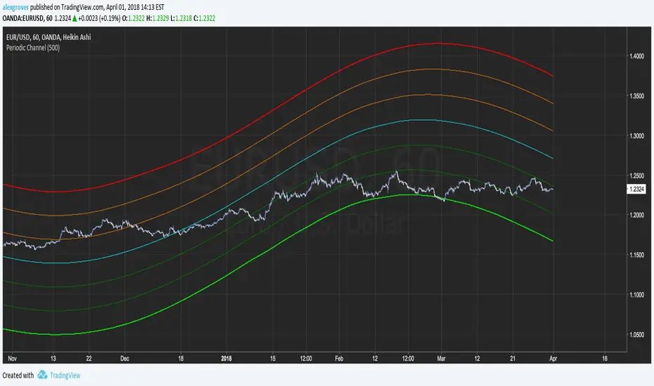
Periodic ChannelThis indicator try to create a channel by summing a re-scaled and readapted sinusoidal wave form to the price mean.
The length parameter control the speed of the sinusoidal wave form, this parameter is not converted to a sine wave period for allowing a better estimation, higher length's work better but feel free to try shorter periods.
The invert parameter invert the sinusoidal wave.
Each bands represent possible return points, the higher the band the higher the probability.
Inverted sin wave exemple
The performance of the indicator is subjective to the main estimation (blue line), select the parameter that best fit the blue line to the price.
Best ragards
Cari dalam skrip untuk "wave"
rem sim v0.1every alt-coin has similarity.
cause of bitcoin.
always i want to delete that similarity and read the true(?) value of each coin.
and i made some script for that, but not good enough.
this one is different.
Rem Sim (rs) removes the similarity very effectively.
it make avg WaveTrend from nxt, strat, steem, ...
and that is the similarity
and it show true(?) WaveTrend without similarity.
so if the alt-coin move like other alt-coin, the WT almost 0.
sorry my bad english.
if you dont understand my english. just look at that chart.
also you can see source code.
--------
대부분의 알트가 어느정도 비슷한 차트를 가지는데, 그 유사성을 제거하면 어떤 모양인지 궁금해서 만들었어요.
전에 만들었던 비트코인의 영향력을 제거해주는 아이디어는 실제론 별 효용이 없는데 이건 좀 쓸만해보이네요.
웨이브트렌드의 모양으로 보여줍니다.

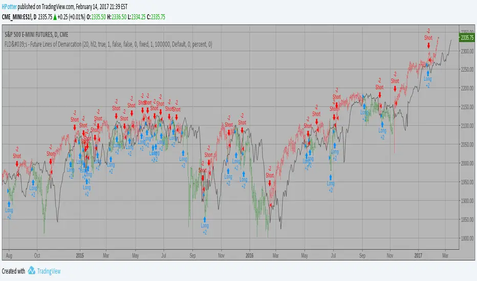
FLD's - Future Lines of Demarcation Backtest An FLD is a line that is plotted on the same scale as the price and is in fact the
price itself displaced to the right (into the future) by (approximately) half the
wavelength of the cycle for which the FLD is plotted. There are three FLD's that can be
plotted for each cycle:
An FLD based on the median price.
An FLD based on the high price.
An FLD based on the low price.
FLD - Future Lines of Demarcation Strategy An FLD is a line that is plotted on the same scale as the price and is in fact the
price itself displaced to the right (into the future) by (approximately) half the
wavelength of the cycle for which the FLD is plotted. There are three FLD's that can be
plotted for each cycle:
An FLD based on the median price.
An FLD based on the high price.
An FLD based on the low price.

FLD's - Future Lines of Demarcation An FLD is a line that is plotted on the same scale as the price and is in fact the
price itself displaced to the right (into the future) by (approximately) half the
wavelength of the cycle for which the FLD is plotted. There are three FLD's that can be
plotted for each cycle:
An FLD based on the median price.
An FLD based on the high price.
An FLD based on the low price.

EDUVEST Lorentzian ClassificationEDUVEST Lorentzian Classification - Machine Learning Signal Detection
━━━━━━━━━━━━━━━━━━━━━━━━━━━━━━━━━━━━━━━━━━━━━━━━
█ ORIGINALITY
This indicator enhances the original Lorentzian Classification concept by jdehorty with EduVest's visual modifications and alert system integration. The core innovation is using Lorentzian distance instead of Euclidean distance for k-NN classification, providing more robust pattern recognition in financial markets.
━━━━━━━━━━━━━━━━━━━━━━━━━━━━━━━━━━━━━━━━━━━━━━━━
█ WHAT IT DOES
- Generates BUY/SELL signals using machine learning classification
- Displays kernel regression estimate for trend visualization
- Shows prediction values on each bar
- Provides trade statistics (Win Rate, W/L Ratio)
- Includes multiple filter options (Volatility, Regime, ADX, EMA, SMA)
━━━━━━━━━━━━━━━━━━━━━━━━━━━━━━━━━━━━━━━━━━━━━━━━
█ HOW IT WORKS
【Lorentzian Distance Calculation】
Unlike Euclidean distance, Lorentzian distance uses logarithmic transformation:
d = Σ log(1 + |xi - yi|)
This provides:
- Better handling of outliers
- More stable distance measurements
- Reduced sensitivity to extreme values
【Feature Engineering】
The classifier uses up to 5 configurable features:
- RSI (Relative Strength Index)
- WT (WaveTrend)
- CCI (Commodity Channel Index)
- ADX (Average Directional Index)
Each feature is normalized using the n_rsi, n_wt, n_cci, or n_adx functions.
【k-Nearest Neighbors Classification】
1. Calculate Lorentzian distance between current bar and historical bars
2. Find k nearest neighbors (default: 8)
3. Sum predictions from neighbors
4. Generate signal based on prediction sum (>0 = Long, <0 = Short)
【Kernel Regression】
Uses Rational Quadratic kernel for smooth trend estimation:
- Lookback Window: 8
- Relative Weighting: 8
- Regression Level: 25
【Filters】
- Volatility Filter: Filters signals during extreme volatility
- Regime Filter: Identifies market regime using threshold
- ADX Filter: Confirms trend strength
- EMA/SMA Filter: Trend direction confirmation
━━━━━━━━━━━━━━━━━━━━━━━━━━━━━━━━━━━━━━━━━━━━━━━━
█ HOW TO USE
【Recommended Settings】
- Timeframe: 15M, 1H, 4H, Daily
- Neighbors Count: 8 (default)
- Feature Count: 5 for comprehensive analysis
【Signal Interpretation】
- Green BUY label: Long entry signal
- Red SELL label: Short entry signal
- Bar colors: Green (bullish) / Red (bearish) prediction strength
【Trade Statistics Panel】
- Winrate: Historical win percentage
- Trades: Total (Wins|Losses)
- WL Ratio: Win/Loss ratio
- Early Signal Flips: Premature signal changes
【Filter Recommendations】
- Enable Volatility Filter for ranging markets
- Enable Regime Filter for trend confirmation
- Use EMA Filter (200) for higher timeframes
━━━━━━━━━━━━━━━━━━━━━━━━━━━━━━━━━━━━━━━━━━━━━━━━
█ CREDITS
Original Lorentzian Classification concept and MLExtensions library by jdehorty.
Enhanced with visual modifications and alert integration by EduVest.
License: Mozilla Public License 2.0

Fractal Market Geometry [JOAT]
Fractal Market Geometry
Overview
Fractal Market Geometry is an open-source overlay indicator that combines fractal analysis with harmonic pattern detection, Fibonacci retracements and extensions, Elliott Wave concepts, and Wyckoff phase identification. It provides traders with a geometric framework for understanding market structure and identifying potential reversal patterns with multi-factor signal confirmation.
What This Indicator Does
The indicator calculates and displays:
Fractal Detection - Identifies fractal highs and lows using Williams-style pivot analysis with configurable period
Fractal Dimension - Calculates market complexity using range-based dimension estimation
Harmonic Patterns - Detects Gartley, Butterfly, Bat, Crab, Shark, Cypher, and ABCD patterns using Fibonacci ratios
Fibonacci Retracements - Key levels at 38.2%, 50%, and 61.8%
Fibonacci Extensions - Projection level at 161.8%
Elliott Wave Count - Simplified wave counting based on pivot detection (1-5)
Wyckoff Phase - Volume-based phase identification (Accumulation, Markup, Distribution, Neutral)
Golden Spiral Levels - ATR-based support and resistance levels using phi (1.618) ratio
Trend Detection - EMA crossover trend identification (20/50 EMA)
How It Works
Fractal detection uses a configurable period to identify swing points:
detectFractalHigh(simple int period) =>
bool result = true
float centerVal = high
for i = 0 to period - 1
if high >= centerVal or high >= centerVal
result := false
break
Harmonic pattern detection uses Fibonacci ratio analysis between swing points. Each pattern has specific ratio requirements:
Gartley: AB 0.382-0.618, BC 0.382-0.886, CD 1.27-1.618
Butterfly: AB 0.382-0.5, BC 0.382-0.886, CD 1.618-2.24
Bat: AB 0.5-0.618, BC 1.13-1.618, CD 1.618-2.24
Crab: AB 0.382-0.618, BC 0.382-0.886, CD 2.24-3.618
Shark: AB 0.382-0.618, BC 1.13-1.618, CD 1.618-2.24
Cypher: AB 0.382-0.618, BC 1.13-1.414, CD 0.786-0.886
Wyckoff phase detection analyzes volume relative to price movement:
wyckoffPhase(simple int period) =>
float avgVol = ta.sma(volume, period)
float priceChg = ta.change(close, period)
string phase = "NEUTRAL"
if volume > avgVol * 1.5 and math.abs(priceChg) < close * 0.02
phase := "ACCUMULATION"
else if volume > avgVol * 1.5 and math.abs(priceChg) > close * 0.05
phase := "MARKUP"
else if volume < avgVol * 0.7
phase := "DISTRIBUTION"
phase
Signal Generation
Signals use multi-factor confirmation for accuracy:
BUY Signal: Fractal low + Uptrend (EMA20 > EMA50) + RSI 30-55 + Bullish candle + Volume confirmation
SELL Signal: Fractal high + Downtrend (EMA20 < EMA50) + RSI 45-70 + Bearish candle + Volume confirmation
Pattern Detection: Label appears when harmonic pattern completes at current bar
Dashboard Panel (Top-Right)
Dimension - Fractal dimension value (market complexity measure)
Last High - Most recent fractal high price
Last Low - Most recent fractal low price
Pattern - Current harmonic pattern name or NONE
Elliott Wave - Current wave count (Wave 1-5) or OFF
Wyckoff - Current market phase or OFF
Trend - BULLISH, BEARISH, or NEUTRAL based on EMA crossover
Signal - BUY, SELL, or WAIT status
Visual Elements
Fractal Markers - Small triangles at fractal highs (down arrow) and lows (up arrow)
Geometry Lines - Dashed lines connecting the most recent fractal high and low
Fibonacci Levels - Clean horizontal lines at 38.2%, 50%, and 61.8% retracement levels
Fibonacci Extension - Horizontal line at 161.8% extension level
Golden Spiral Levels - Support and resistance lines based on ATR x 1.618
3D Fractal Field - Optional depth layers around swing levels (OFF by default)
Harmonic Pattern Markers - Small diamond shapes when Crab, Shark, or Cypher patterns detected
Pattern Labels - Text label showing pattern name when detected
Signal Labels - BUY/SELL labels on confirmed multi-factor signals
Input Parameters
Fractal Period (default: 5) - Bars on each side for fractal detection
Geometry Depth (default: 3) - Complexity of geometric calculations
Pattern Sensitivity (default: 0.8) - Tolerance for pattern ratio matching
Show Fibonacci Levels (default: true) - Display retracement levels
Show Fibonacci Extensions (default: true) - Display extension level
Elliott Wave Detection (default: true) - Enable wave counting
Wyckoff Analysis (default: true) - Enable phase detection
Golden Spiral Levels (default: true) - Display spiral support/resistance
Show Fractal Points (default: true) - Display fractal markers
Show Geometry Lines (default: true) - Display connecting lines
Show Pattern Labels (default: true) - Display pattern name labels
Show 3D Fractal Field (default: false) - Display depth layers
Show Harmonic Patterns (default: true) - Display pattern markers
Show Buy/Sell Signals (default: true) - Display signal labels
Suggested Use Cases
Identify potential reversal zones using harmonic pattern completion
Use Fibonacci levels for entry, stop-loss, and target planning
Monitor Wyckoff phases for accumulation/distribution awareness
Track Elliott Wave counts for trend structure analysis
Use fractal dimension to gauge market complexity
Wait for multi-factor signal confirmation before entering trades
Timeframe Recommendations
Best on 1H to Daily charts. Lower timeframes produce more fractals but with less significance. Higher timeframes provide stronger levels and more reliable signals.
Limitations
Harmonic pattern detection uses simplified ratio ranges and may not match all textbook definitions
Elliott Wave counting is basic and does not include all wave rules
Wyckoff phase detection is volume-based approximation
Fractal dimension calculation is simplified
Signals require fractal confirmation which has inherent lag equal to the fractal period
Open-Source and Disclaimer
This script is published as open-source under the Mozilla Public License 2.0 for educational purposes. It does not constitute financial advice. Past performance does not guarantee future results. Always use proper risk management.
- Made with passion by officialjackofalltrades

Nuh's Complete Multi-Timeframe Dashboard v4.0Nuh's Complete Multi-Timeframe Dashboard v4.0 - Unified Power System
Professional Multi-Timeframe Technical Analysis Dashboard
Nuh's Complete Multi-Timeframe Dashboard v4.0 represents a comprehensive trading analysis system that unifies 20 powerful technical indicators across up to 6 customizable timeframes into a single, intelligent dashboard. This advanced indicator combines trend analysis (EMA, Alpha Trend, SuperTrend, ADX, DI), momentum oscillators (RSI, Stochastic RSI, MACD, CCI, Williams %R, WaveTrend, KST), volume indicators (OBV, CMF, Volume Analysis, MFI), and volatility measures (Squeeze Momentum, Bollinger Bands, ATR, Williams VIX Fix) to provide traders with a holistic market perspective. Each indicator can be independently enabled or disabled, allowing complete customization based on your trading strategy and preferences.
The revolutionary Weighted Power System is the core innovation of this dashboard, transforming raw indicator signals into actionable market power scores. Unlike traditional dashboards that simply count bullish or bearish signals, this system applies sophisticated weighting to each indicator based on your chosen preset (Balanced, Trend Focus, Momentum Focus, Volume Focus) or custom weights. It then combines these weighted signals across multiple timeframes—with timeframe-specific weighting for scalping, day trading, or swing trading styles—to calculate an Overall Market Power score. This provides you with clear percentage-based bullish and bearish power readings, eliminating guesswork and enabling confident trade decisions backed by mathematical confluence.
Built for serious traders who demand precision and flexibility, the dashboard features a fully customizable display with 20 indicator rows that can be reordered to match your preferences, color-coded gradient visualization for instant market sentiment recognition, and integrated Wundertrading-compatible alerts for automated trading. The system supports both legacy count-based alerts and modern power-threshold alerts, allowing you to receive notifications when market conditions meet your specified confluence requirements. Whether you're scalping on lower timeframes or swing trading on higher timeframes, this professional-grade tool adapts to your trading style while maintaining clean, readable visualization that won't clutter your charts.

Confluence Execution Engine (2of3)The Confluence Execution Engine is a high-performance logic gate designed to filter out market noise and identify high-probability "Golden" entries. It moves beyond simple indicator signals by acting as a mathematical validator for price action. This engine is designed for the Systematic Trader. It removes the "guesswork" of whether a move is real or an exhaustion pump by requiring a mathematical confluence of volume, multi-timeframe momentum, and volatility-adjusted space.
Why This Tool is Unique:
Multi-Dimensional Scoring, Momentum-Adjusted Stretch, Institutional Fingerprint (RVOL + Spike)
Unlike a standard MACD or RSI, this engine uses a weighted scoring matrix. It pulls a "Bundle" of data (WaveTrend, RSI, ROC) from four different timeframes simultaneously. It doesn't give a signal unless the mathematical weight of all four timeframes crosses your "Hurdle" (Base Threshold).
Standard "overbought" indicators are often wrong during strong trends. This engine uses Dynamic Z-Score logic. The Logic: If the price moves away from the mean, it checks the Rate of Change (ROC). The Result: If momentum is massive, the "Stretch" limit expands. It understands that a "stretched" price is actually a sign of strength in a breakout, not a reason to exit. It only warns of a TRAP RISK when the price is far from the mean but momentum is starting to stall.
The engine is gated by Relative Volume. If the market is "sleepy," the engine stays in "PATIENCE" mode. It specifically hunts for Volume Spikes (default 2.5x average). A signal is only upgraded to "HIGH CONVICTION" when an institutional volume spike occurs, confirming that "Big Money" is participating.
How to Operate the Engine
Define Your Hurdle: Set your Confluence Hurdle. A higher number (e.g., 14+) requires more agreement across timeframes, leading to fewer but higher-quality trades.
Monitor the Z/Dynamic Ratio: In the HUD, watch the Z: X.XX / Y.YY. When X approaches Y, you are reaching the edge of the momentum-adjusted move.
The Entry Trigger: Wait for a "LOOK FOR..." advice to turn into a "HIGH CONVICTION" signal (marked by a triangle shape). This confirms that the MTF scoring, Volume, and HTF Trend are all aligned.
Execute the Lines: Use the red and green "Ghost Lines" to set your orders. These are ATR-based, meaning they widen during high volatility to give your trade room to breathe.
For holistic trading system, pair with Volatility Shield Pro and Session Levels

Supply-Demand Dominance & Energy RibbonOverview:
This indicator is specifically fine-tuned for the Nasdaq (NAS100) market. It combines volume-based Delta analysis (Supply-Demand) with price kinetic energy (Slope) to identify high-probability reversal points and trend strength.
Key Features & Usage:
Supply-Demand Dominance (Top-Right Label):
Analyzes volume spikes over a 50-period lookback to determine market control.
Displays "매수 우위" (Bullish Dominance) or "매도 우위" (Bearish Dominance) in real-time.
Energy Ribbon (Bottom Visualization):
Calculates the slope of the TCI oscillator to visualize momentum intensity.
Solid Green/Red: Strong momentum.
Faded Green/Red: Weakening momentum or minor trend.
Momentum Combo Signals (Circle Shapes):
Triggered when WaveTrend and TCI oscillators cross in extreme zones (Overbought 70 / Oversold 30).
Smart Filter: Signals are only shown when they align with the current Supply-Demand dominance, reducing "market noise."
Volume Spikes (Arrow Symbols):
Indicates abnormal volume activity (1.5x average delta). These arrows (↑/↓) help identify potential breakout points or the climax of a move even when a full combo signal isn't present.

All-in-One Momentum Composite The Four Components (and Why They're Chosen)
RSI (Relative Strength Index) – Classic overbought/oversold oscillator (14-period default). Measures speed and change of price movements.
Stochastic (%D line) – Smoothened momentum indicator that compares closing price to the price range over a period. Excellent at spotting reversals in ranging markets.
WaveTrend – Very popular in crypto and forex communities (originally by LazyBear). It’s essentially a momentum oscillator based on overbought/oversold channels, similar to a faster, smoother RSI/Stochastic hybrid. Known for early divergence signals and clean crossovers.
MACD Histogram – Captures momentum changes and trend strength via the difference between fast and slow EMAs. The histogram shows acceleration/deceleration.

Volatility Aurora [The_lurker]█░░░░░░░░░░░░░░░░░░░ VOLATILITY AURORA ░░░░░░░░░░░░░░░░░░░░█
█░░░░░░░░░░░░░░░ Where Market Energy Meets Visual Poetry ░░░░░░░░░░░░░░░░█
📖 INTRODUCTION
━━━━━━━━━━━━━━━━━━━━━━━━━━━━━━━━━━━━━━━━━━━
The Aurora Borealis occurs when charged particles from the sun collide with gases in Earth's atmosphere, creating mesmerizing waves of colorful light.
𝗩𝗼𝗹𝗮𝘁𝗶𝗹𝗶𝘁𝘆 𝗔𝘂𝗿𝗼𝗿𝗮 applies this elegant concept to financial markets:
⚡ Price Momentum = Charged Particles
🌌 ATR Layers = Atmospheric Layers
🎨 Color Intensity = Energy Magnitude
📐 Layer Expansion = Volatility State
When momentum "collides" with volatility layers, the Aurora illuminates potential market regime changes — often before they fully manifest in price action.
🔬 THE SCIENCE BEHIND IT
━━━━━━━━━━━━━━━━━━━━━━━━━━━━━━━━━━━━━━━━━━━━━━━━━━━━━━━━━━━━━━━━━━━━━━━━━━━━━
Unlike traditional volatility indicators that provide a single value, Volatility Aurora creates a 𝗺𝘂𝗹𝘁𝗶-𝗱𝗶𝗺𝗲𝗻𝘀𝗶𝗼𝗻𝗮𝗹 𝘃𝗼𝗹𝗮𝘁𝗶𝗹𝗶𝘁𝘆 𝗳𝗶𝗲𝗹𝗱 using five distinct ATR layers based on Fibonacci periods:
│ Layer │ Period │ Atmospheric │ Function │
├──────────────────────┼─────────────────┼─────────────────┤
│ Layer 1 │ 5 │ Ionosphere │ Captures immediate vol shifts
│ Layer 2 │ 13 │ Mesosphere │ Medium-term vol response
│ Layer 3 │ 34 │ Stratosphere │ Intermediate vol structure
│ Layer 4 │ 55 │ Troposphere │ Foundational vol baseline
│ Layer 5 │ 89 │ Surface │ Structural, long-term vol
⚡ CORE CONCEPTS
━━━━━━━━━━━━━━━━━━━━━━━━━━━━━━━━━━━━━━━━━━━
𝟭. 𝗟𝗮𝘆𝗲𝗿 𝗘𝘅𝗽𝗮𝗻𝘀𝗶𝗼𝗻 & 𝗖𝗼𝗻𝘁𝗿𝗮𝗰𝘁𝗶𝗼𝗻
Each layer dynamically expands or contracts based on its normalized ATR value:
• 𝗘𝘅𝗽𝗮𝗻𝗱𝗶𝗻𝗴 𝗟𝗮𝘆𝗲𝗿𝘀 → Increasing volatility regime
• 𝗖𝗼𝗻𝘁𝗿𝗮𝗰𝘁𝗶𝗻𝗴 𝗟𝗮𝘆𝗲𝗿𝘀 → Decreasing volatility / Consolidation
• 𝗕𝗿𝗲𝗮𝘁𝗵𝗶𝗻𝗴 𝗘𝗳𝗳𝗲𝗰𝘁 → Natural market rhythm visualization
𝟮. 𝗛𝗮𝗿𝗺𝗼𝗻𝘆 𝗦𝗰𝗼𝗿𝗲
Measures alignment between all five layers:
• 𝗛𝗶𝗴𝗵 𝗛𝗮𝗿𝗺𝗼𝗻𝘆 (>70%) → All timeframes agree → Strong, reliable trends
• 𝗟𝗼𝘄 𝗛𝗮𝗿𝗺𝗼𝗻𝘆 (<30%) → Timeframe divergence → Choppy conditions
𝟯. 𝗘𝗻𝗲𝗿𝗴𝘆 𝗜𝗻𝘁𝗲𝗻𝘀𝗶𝘁𝘆
Quantifies how strongly momentum is "hitting" the volatility layers:
• 𝗛𝗶𝗴𝗵 𝗜𝗻𝘁𝗲𝗻𝘀𝗶𝘁𝘆 → Strong directional conviction
• 𝗟𝗼𝘄 𝗜𝗻𝘁𝗲𝗻𝘀𝗶𝘁𝘆 → Weak momentum, potential reversal
𝟰. 𝗥𝗲𝗴𝗶𝗺𝗲 𝗖𝗹𝗮𝘀𝘀𝗶𝗳𝗶𝗰𝗮𝘁𝗶𝗼𝗻
Based on aggregate layer states:
🟢 𝗖𝗔𝗟𝗠 → Low volatility across all layers
🟡 𝗡𝗢𝗥𝗠𝗔𝗟 → Balanced market conditions
🟠 𝗩𝗢𝗟𝗔𝗧𝗜𝗟𝗘 → Elevated activity
🔴 𝗘𝗫𝗧𝗥𝗘𝗠𝗘 → Maximum volatility state
🎨 VISUAL COMPONENTS
━━━━━━━━━━━━━━━━━━━━━━━━━━━━━━━━━━━━━━━━━━━
🌈 𝗔𝘂𝗿𝗼𝗿𝗮 𝗟𝗮𝘆𝗲𝗿𝘀 (𝗚𝗿𝗮𝗱𝗶𝗲𝗻𝘁 𝗕𝗮𝗻𝗱𝘀)
• Five pairs of symmetrical bands around the price core
• Color gradient from core (bright) to outer (dim)
• Expansion reflects current volatility state
💠 𝗖𝗼𝗿𝗲 𝗟𝗶𝗻𝗲
• Central EMA-based trend line
• Color changes with momentum direction:
🟢 Cyan/Teal = Bullish
🔴 Pink/Magenta = Bearish
🟣 Purple = Neutral
💫 𝗘𝗻𝗲𝗿𝗴𝘆 𝗣𝘂𝗹𝘀𝗲 𝗟𝗶𝗻𝗲𝘀
• Diagonal flow lines showing momentum trajectory
• Thicker lines = Higher energy
• Direction indicates momentum flow
🎵 𝗛𝗮𝗿𝗺𝗼𝗻𝘆 𝗪𝗮𝘃𝗲𝘀
• Vertical dotted lines appear when harmony exceeds 70%
• Signals timeframe alignment — high-probability zones
📊 HOW TO USE
━━━━━━━━━━━━━━━━━━━━━━━━━━━━━━━━━━━━━━━━━━━
📈 𝗧𝗿𝗲𝗻𝗱 𝗙𝗼𝗹𝗹𝗼𝘄𝗶𝗻𝗴
• Enter when Aurora expands in your direction
• Core line color confirms bias
• High harmony = Higher confidence
💥 𝗩𝗼𝗹𝗮𝘁𝗶𝗹𝗶𝘁𝘆 𝗕𝗿𝗲𝗮𝗸𝗼𝘂𝘁𝘀
• Watch for regime shift from CALM to VOLATILE
• Expanding layers signal incoming movement
• Intensity spike confirms breakout strength
↩️ 𝗠𝗲𝗮𝗻 𝗥𝗲𝘃𝗲𝗿𝘀𝗶𝗼𝗻
• EXTREME regime often precedes reversals
• Contracting layers after expansion = Potential pullback
• Low harmony during trends = Weakening momentum
🛡️ 𝗥𝗶𝘀𝗸 𝗠𝗮𝗻𝗮𝗴𝗲𝗺𝗲𝗻𝘁
• Use outer layers as dynamic support/resistance
• Wider Aurora = Wider stops required
• Contracting Aurora = Tighter risk parameters
⚙️ SETTINGS GUIDE
━━━━━━━━━━━━━━━━━━━━━━━━━━━━━━━━━━━━━━━━━━━
🌌 𝗔𝘂𝗿𝗼𝗿𝗮 𝗖𝗼𝗿𝗲
│ Setting │Default │ Description
│ Layer 1-5 │ Fib │ ATR periods (5,13,34,55,89)
│ Expansion Factor │ 2.5 │ Controls layer width multiplier
│ Smoothing │ 5 │ EMA smoothing for visual clarity
⚡ 𝗘𝗻𝗲𝗿𝗴𝘆 𝗙𝗶𝗲𝗹𝗱
│ Setting │ Default │ Description
│ Momentum Length │ 14 │ Period for momentum calculation
│ Energy Lookback │ 21 │ Normalization window
│ Energy Multiplier │ 1.5 │ Amplifies energy display
🎨 𝗩𝗶𝘀𝘂𝗮𝗹
│ Setting │ Default │ Description
│ Language │ EN │ Interface language (EN/AR)
│ Show Aurora │ ✓ │ Toggle layer visibility
│ Show Core Line │ ✓ │ Toggle center line
│ Show Energy Pulse │ ✓ │ Toggle flow lines
│ Show Harmony Waves │ ✓ │ Toggle alignment indicators
🔔 ALERTS
━━━━━━━━━━━━━━━━━━━━━━━━━━━━━━━━━━━━━━━━━━━
⚡ 𝗥𝗲𝗴𝗶𝗺𝗲 𝗦𝗵𝗶𝗳𝘁 — Volatility regime changed
🎵 𝗛𝗶𝗴𝗵 𝗛𝗮𝗿𝗺𝗼𝗻𝘆 — All layers aligned (>85%)
↕️ 𝗗𝗶𝗿𝗲𝗰𝘁𝗶𝗼𝗻 𝗖𝗵𝗮𝗻𝗴𝗲 — Momentum direction reversed
🔥 𝗜𝗻𝘁𝗲𝗻𝘀𝗶𝘁𝘆 𝗦𝗽𝗶𝗸𝗲 — Energy exceeded 80% threshold
💡 TIPS FOR BEST RESULTS
━━━━━━━━━━━━━━━━━━━━━━━━━━━━━━━━━━━━━━━━━━━
1️⃣ 𝗛𝗶𝗴𝗵𝗲𝗿 𝗧𝗶𝗺𝗲𝗳𝗿𝗮𝗺𝗲𝘀 — Aurora works best on 1H+ charts
2️⃣ 𝗖𝗼𝗺𝗯𝗶𝗻𝗲 𝘄𝗶𝘁𝗵 𝗣𝗔 — Use Aurora as context, not signals
3️⃣ 𝗪𝗮𝘁𝗰𝗵 𝗛𝗮𝗿𝗺𝗼𝗻𝘆 — High harmony setups win more
4️⃣ 𝗥𝗲𝘀𝗽𝗲𝗰𝘁 𝗥𝗲𝗴𝗶𝗺𝗲 — Don't fight EXTREME volatility
5️⃣ 𝗟𝗮𝘆𝗲𝗿 𝗖𝗼𝗻𝗳𝗹𝘂𝗲𝗻𝗰𝗲 — Multi-layer bounces = Strong S/R
⚠️ DISCLAIMER
━━━━━━━━━━━━━━━━━━━━━━━━━━━━━━━━━━━━━━━━━━━
This indicator is for educational purposes only. Past performance does not
guarantee future results. Always use proper risk management and conduct your
own analysis before making trading decisions.
█████████████████████████████████████████████████████████████
█░░░░░░░░░░░░░░░░░░░░░ شفق التقلب ░░░░░░░░░░░░░░░░░░░░░░█
█░░░░░░░░░░░░░░░ حيث تلتقي طاقة السوق بالشعور البصري ░░░░░░░░░░░░░░░░█
📖 المقدمة
━━━━━━━━━━━━━━━━━━━━━━━━━━━━━━━━━━━━━━━━━━━
يحدث الشفق القطبي عندما تصطدم الجسيمات المشحونة القادمة من الشمس بالغازات في الغلاف الجوي للأرض، مما يخلق موجات ساحرة من الضوء الملون.
يطبق نفس المفهوم الأنيق على الأسواق المالية
⚡ زخم السعر = الجسيمات المشحونة
🌌 طبقات ATR = طبقات الغلاف الجوي
🎨 شدة اللون = حجم الطاقة
📐 توسع الطبقات = حالة التقلب
عندما "يصطدم" الزخم بطبقات التقلب، يُضيء الشفق التغيرات المحتملة في نظام السوق — غالباً قبل أن تتجلى بالكامل في حركة السعر.
🔬 العلم وراء المؤشر
━━━━━━━━━━━━━━━━━━━━━━━━━━━━━━━━━━━━━━━━━━━
على عكس مؤشرات التقلب التقليدية التي تقدم قيمة واحدة، يُنشئ شفق التقلب 𝗽𝗮𝗾𝗹 𝘁𝗮𝗾𝗮𝗹𝗹𝘂𝗯 𝗺𝘂𝘁𝗮'𝗮𝗱𝗱𝗶𝗱 𝗮𝗹-𝗮𝗯'𝗮𝗱 باستخدام خمس طبقات ATR مميزة مبنية على أرقام فيبوناتشي:
│ الطبقة │ الفترة │ المعادل الجوي │ الوظيفة
│ الطبقة١ │ 5 │ الأيونوسفير │ تلتقط تحولات التقلب الفورية
│ الطبقة٢ │ 13 │ الميزوسفير │ استجابة التقلب متوسطة المدى
│ الطبقة٣ │ 34 │ الستراتوسفير │ هيكل التقلب المتوسط
│ الطبقة٤ │ 55 │ التروبوسفير │ خط الأساس للتقلب
│ الطبقة٥ │ 89 │ السطح │ التقلب الهيكلي طويل المدى
⚡ المفاهيم الأساسية
━━━━━━━━━━━━━━━━━━━━━━━━━━━━━━━━━━━━━━━━━━━
𝟭. توسع وانكماش الطبقات
تتوسع أو تنكمش كل طبقة ديناميكياً بناءً على قيمة ATR المعيارية:
• طبقات متوسعة ← نظام تقلب متزايد
• طبقات منكمشة ← تقلب متناقص / تجميع
• تأثير التنفس ← تصور إيقاع السوق الطبيعي
𝟮. درجة التناغم
تقيس التوافق بين جميع الطبقات الخمس:
• تناغم عالي (>٧٠٪) ← جميع الأطر متفقة ← اتجاهات قوية
• تناغم منخفض (<٣٠٪) ← تباين الأطر ← ظروف متقطعة
𝟯. شدة الطاقة
تحدد مدى قوة "اصطدام" الزخم بطبقات التقلب:
• شدة عالية ← قناعة اتجاهية قوية
• شدة منخفضة ← زخم ضعيف، احتمال انعكاس
𝟰. تصنيف النظام
بناءً على حالات الطبقات المجمعة:
🟢 هادئ ← تقلب منخفض عبر جميع الطبقات
🟡 طبيعي ← ظروف سوق متوازنة
🟠 متقلب ← نشاط مرتفع
🔴 متطرف ← حالة التقلب القصوى
🎨 المكونات البصرية
━━━━━━━━━━━━━━━━━━━━━━━━━━━━━━━━━━━━━━━━━━━
🌈 طبقات الشفق (النطاقات المتدرجة)
• خمسة أزواج من النطاقات المتماثلة حول نواة السعر
• تدرج لوني من النواة (ساطع) إلى الخارج (خافت)
• التوسع يعكس حالة التقلب الحالية
💠 خط النواة
• خط اتجاه مركزي قائم على EMA
• يتغير اللون مع اتجاه الزخم:
🟢 سماوي = صاعد
🔴 وردي = هابط
🟣 بنفسجي = محايد
💫 خطوط نبض الطاقة
• خطوط تدفق مائلة تُظهر مسار الزخم
• خطوط أسمك = طاقة أعلى
• الاتجاه يشير إلى تدفق الزخم
🎵 موجات التناغم
• خطوط عمودية منقطة تظهر عندما يتجاوز التناغم ٧٠٪
• تشير إلى توافق الأطر الزمنية — مناطق احتمالية عالية
📊 كيفية الاستخدام
━━━━━━━━━━━━━━━━━━━━━━━━━━━━━━━━━━━━━━━━━━━
📈 تتبع الاتجاه
• ادخل عندما يتوسع الشفق في اتجاهك
• لون خط النواة يؤكد التحيز
• تناغم عالي = ثقة أعلى
💥 اختراقات التقلب
• راقب تحول النظام من هادئ إلى متقلب
• الطبقات المتوسعة تشير إلى حركة قادمة
• ارتفاع الشدة يؤكد قوة الاختراق
↩️ الارتداد للمتوسط
• النظام المتطرف غالباً يسبق الانعكاسات
• طبقات منكمشة بعد التوسع = احتمال تراجع
• تناغم منخفض أثناء الاتجاهات = زخم ضعيف
🛡️ إدارة المخاطر
• استخدم الطبقات الخارجية كدعم/مقاومة ديناميكية
• شفق أوسع = وقف خسارة أوسع مطلوب
• شفق منكمش = معايير مخاطر أضيق
⚙️ دليل الإعدادات
━━━━━━━━━━━━━━━━━━━━━━━━━━━━━━━━━━━━━━━━━━━
🌌 نواة الشفق
│ الإعداد │الافتراضي│ الوصف
│ الطبقات ١-٥ │ Fib │ فترات ATR (5,13,34,55,89)
│ معامل التوسع │ 2.5 │ يتحكم في مضاعف عرض الطبقات
│ التنعيم │ 5 │ تنعيم EMA للوضوح البصري
⚡ مجال الطاقة
│ الإعداد │الافتراضي│ الوصف
│ فترة الزخم │ 14 │ فترة حساب الزخم
│ فترة الطاقة │ 21 │ نافذة التطبيع
│ مضاعف الطاقة │ 1.5 │ يضخم عرض الطاقة
🎨 العرض البصري
│ الإعداد │الافتراضي│ الوصف
│ اللغة │ EN │ لغة الواجهة (EN/AR)
│ إظهار الشفق │ ✓ │ تبديل ظهور الطبقات
│ خط النواة │ ✓ │ تبديل الخط المركزي
│ نبض الطاقة │ ✓ │ تبديل خطوط التدفق
│ موجات التناغم │ ✓ │ تبديل مؤشرات التوافق
🔔 التنبيهات
━━━━━━━━━━━━━━━━━━━━━━━━━━━━━━━━━━━━━━━━━━━
⚡ تحول النظام — تغير نظام التقلب
🎵 تناغم عالي — جميع الطبقات متوافقة (>٨٥٪)
↕️ تغير الاتجاه — انعكس اتجاه الزخم
🔥 ارتفاع الشدة — تجاوزت الطاقة عتبة ٨٠٪
💡 نصائح للحصول على أفضل النتائج
━━━━━━━━━━━━━━━━━━━━━━━━━━━━━━━━━━━━━━━━━━━
1️⃣ الأطر الزمنية الأعلى — الشفق يعمل بشكل أفضل على ساعة فأكثر
2️⃣ ادمج مع حركة السعر — استخدم الشفق كسياق وليس إشارات
3️⃣ راقب التناغم — إعدادات التناغم العالي تربح أكثر
4️⃣ احترم النظام — لا تحارب التقلب المتطرف
5️⃣ تقاطع الطبقات — ارتداد من طبقات متعددة = دعم/مقاومة قوية
⚠️ إخلاء المسؤولية
━━━━━━━━━━━━━━━━━━━━━━━━━━━━━━━━━━━━━━━━━━━
هذا المؤشر للأغراض التعليمية فقط. الأداء السابق لا يضمن النتائج المستقبلية.
استخدم دائماً إدارة مخاطر مناسبة وقم بتحليلك الخاص قبل اتخاذ قرارات التداول.
█████████████████████████████████████████████████████████████

BOS and CHoCHThe market never moves in a straight line. It moves in waves.
It makes a High, comes down a bit (Low), then breaks the previous High to make a new High.
Similarly, It makes a Low, goes up a bit (High), then breaks the previous Low to make a new Low.
BOS (Break Of Structure) - Trend Continuation
BOS means the market is continuing its current trend. If the market is in an Uptrend and breaks the old "High" -> Bullish BOS. If the market is in a Downtrend and breaks the old "Low" -> Bearish BOS.
3. CHOCH (Change Of Character) - Trend Reversal
CHOCH means the mood of the market has changed. For the first time, the trend has shifted its nature.
Bullish to Bearish CHOCH: The market was making Higher Highs, but suddenly it broke its previous "Low". Now the market can fall.
Bearish to Bullish CHOCH: The market was falling (Lower Lows), but suddenly it broke its previous "High". Now the market can rise.
BOS: Confirms the trend (Breaking the ceiling to go higher).
CHOCH: Signals a trend change (Slipping and falling below the previous floor).

QLC v8.4 – GIBAUUM BEAST + ANTI-FAKEOUTQLC v8.4 – GIBAUUM BEAST + ANTI-FAKEOUT
QLC v8.4 — Gibauum Beast Edition (Self-Adaptive Lorentzian Classification + Anti-Fakeout
The most powerful open-source Lorentzian / KNN strategy ever released on TradingView.
Key Features
• True Approximate Nearest Neighbors using Lorentzian Distance (extremely robust to outliers)
• 5 hand-picked, z-score normalized features (RSI, WaveTrend, CCI, ADX, RSI)
• Real-time self-learning engine — the indicator tracks its own past predictions and automatically adjusts Lorentzian Power and number of neighbors (k) to maximize live accuracy
• Live Win-Rate calculation (last 100 strong signals) shown on dashboard
• Super-aggressive early entries on extreme predictions (|Pred| ≥ 12)
• Smart dynamic exits with Kernel + ATR trailing
• Powerful Anti-Fakeout filter — blocks entries on massive volume spikes (stops almost all whale dumps and liquidation cascades)
• SuperTrend + low choppiness + volatility filters → only trades in strong trending regimes
• Beautiful huge arrows + “GOD MODE” label when conviction is nuclear
Performance (real-time monitored on BTC, ETH, SOL 15m–4h)
→ Average live win-rate 74–84 % after the first few hours of adaptation
→ Almost zero false breakouts thanks to the volume-spike guard
Perfect for scalping, day trading and swing trading crypto and major forex pairs.
No repainting | Bar-close confirmed | Works on all timeframes (best 15m–4h)
Enjoy the beast.

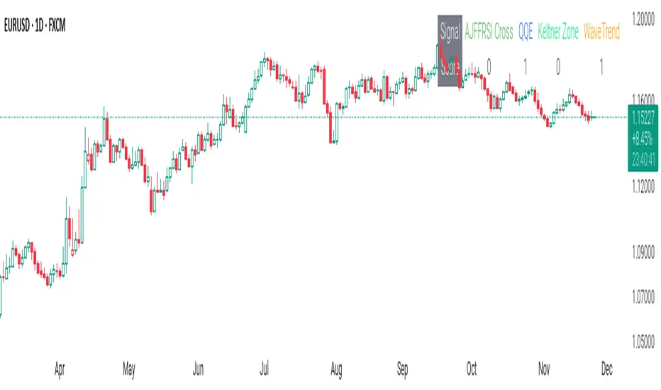
CSS_LFU_v0.1Overview:
A multi-factor, market-adaptive swing strategy designed for intraday and short-term crypto trading. It synthesizes momentum, volatility, and trend signals into a unified composite score over a configurable lookback window. The strategy leverages a modular, signal-weighted approach to ensure robust entry timing while remaining compatible with human-in-the-loop validation and algorithmic execution.
Core Modules:
AJFFRSI (RSX-based Momentum): Measures smoothed price momentum with noise-reduction filters to detect crossovers relative to the QQE trailing stop.
QQE (Quantitative Qualitative Easing RSI): A modified RSI with a dynamic trailing stop that adapts to short-term volatility, identifying exhaustion and potential reversal points.
Keltner Channel Zones: Determines overextension relative to trend, providing buy/sell zones based on ATR-banded EMA.
WaveTrend Oscillator: Confirms short-term swings and market direction through smoothed oscillator cross signals.
Rolling Composite Score: Aggregates module signals over a unified lookback (e.g., 144 bars) to normalize noise and capture consistent trends.
Signal Logic:
Each module outputs a discrete score (+1 / 0 / -1).
The rolling composite score sums all module scores over the lookback period.
Long positions trigger when the rolling score meets or exceeds the long threshold.
Short positions trigger when the rolling score meets or falls below the short threshold.
Multi-dimensional signal aggregation reduces false positives from single indicators.
Rolling lookback ensures score normalization across different volatility regimes.
Highly modular: easy to adapt modules or weights to different instruments or timeframes.
Fully compatible with automated execution pipelines, including custom exchange screener bots.
Use Case:
Ideal for quant-driven altcoin or multi-asset strategies where high-frequency validation is critical and sequential module weighting enhances trend flip detection.
Fib and Slope Trend Detector [EWT] + MTF Dashboard🚀 Overview
The Momentum Structure Trend Detector is a sophisticated trend-following tool that combines Price Velocity (Slope) with Market Structure (Fibonacci) to identify high-probability trend reversals and continuations.
Unlike traditional indicators that rely heavily on lagging moving averages, this script analyzes the speed of price action in real-time. It operates on the core principle of market structure: Impulse moves are fast and steep, while corrections are slow and shallow.
🧠 The Logic: Physics Meets Market Structure
This indicator determines the trend direction by calculating the Slope (Velocity) of price swings.
ZigZag Calculation: It first identifies market swings (Highs and Lows) using a standard pivot detection algorithm.
Slope Calculation: It calculates the velocity of every completed leg using the formula: $Slope = \frac{|Price Change|}{|Time Duration|}$.
Trend Definition:
Uptrend : If the previous Up-move was fast (Impulse) and the subsequent Down-move is slower (Correction), the market is primed for an uptrend.
Downtrend : If the previous Down-move was fast (Impulse) and the subsequent Up-move is slower (Correction), the market is primed for a downtrend.
🔥 Key Features
1. Aggressive Real-Time Detection (No Lag)
Most structure indicators wait for a "Higher High" to confirm a trend, which often leads to late entries. This script uses an Aggressive Live Slope calculation:
It compares the current developing slope of the live price action against the slope of the previous completed leg.
Result: As soon as the current move becomes "steeper" (faster) than the previous correction, the trend flips immediately. This allows you to catch the "meat" of the move before a new pivot is even confirmed.
2. Fibonacci Validity Filter
Momentum alone isn't enough; we need structural integrity.
The script calculates the 78.6% Retracement level of the impulse leg.
If a correction moves deeper than this Fibonacci limit (on a closing basis), the trend structure is considered "broken" or "invalid," and the indicator switches to a Neutral state. This filters out choppy/ranging markets.
3. Multi-Timeframe (MTF) Dashboard
A customizable dashboard on the chart allows for fractal analysis. You can view the trend state (UP/DOWN/NEUTRAL) across 9 different timeframes (1m to 1M) simultaneously.
Green Row : Uptrend
Red Row : Downtrend
Gray : Neutral/Indeterminate
4. Smart Visuals
Background Colo r: Changes dynamically (Teal for Bullish, Red for Bearish, Gray for Neutral) to give you an instant read of the market state.
Slope Labels : Displays the calculated numeric slope on the chart, helping you visualize the momentum difference between impulse and corrective waves.
Invalidation Levels : Automatically plots the invalidation line (Stop Loss level) based on the market structure.
🛠️ Settings & Inputs
Strategy Settings
Pivot Deviation Length : Sensitivity of the ZigZag calculation (Default: 5). Lower numbers = more sensitive to small swings.
Max Retracement % : The Fibonacci limit for a valid correction (Default: 78.6%).
Min Bars for Live Calc : To prevent noise, the script waits for this many bars after a pivot before calculating the "Live Slope" (Default: 3).
Dashboard Settings
Show Dashboard : Toggle the table on/off.
Timeframe Toggles : Enable/Disable specific timeframes (1m, 5m, 15m, 30m, 1H, 4H, 1D, 1W, 1M) to suit your trading style.
🎯 How to Use
Wait for Background Change : When the background turns Teal, it indicates that a corrective pullback has ended and a new impulse with high velocity has begun.
Check Invalidation : Look at the plotted Stop Loss Level. If price closes below this line, the trade idea is invalid.
Confirm with Dashboard : Use the table to ensure the higher timeframes (e.g., 1H, 4H) align with your current chart's direction for higher probability setups.
Disclaimer : This tool is designed for trend analysis and educational purposes. Past performance (momentum) is not indicative of future results. Always manage your risk.

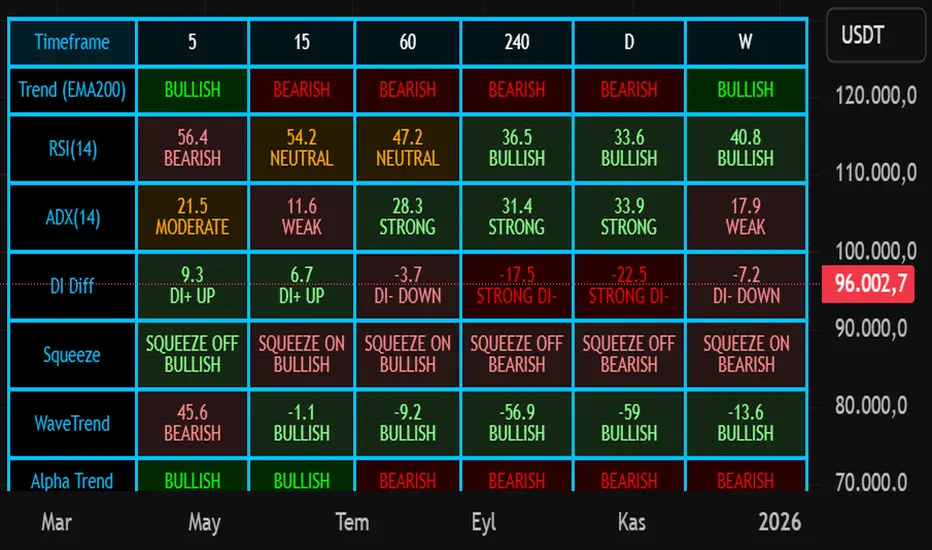
Nuh's Multi-Timeframe DashboardAll 10 indicators (EMA, RSI, ADX, RI, Squeezee, WaveTrend, Alpha Trend, SuperTrend, Stoch RSI, Vix Fix) across 7 time frames (5m, 15m, 1h, 2h, 4h, 1D, 1W) consolidated into a single table.
Cipher B Free | WaveTrend (v6)Uh.. I call this.. Mona Lisa kek. Tried creating my own version of Cipher B with Grok. Feel free to tweak to your heart's content

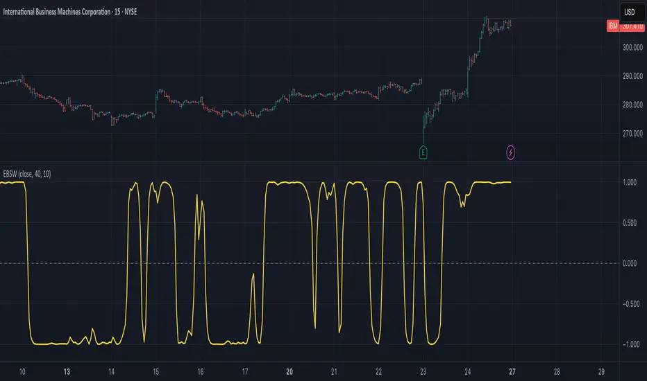
Ehlers Even Better Sinewave (EBSW)# EBSW: Ehlers Even Better Sinewave
## Overview and Purpose
The Ehlers Even Better Sinewave (EBSW) indicator, developed by John Ehlers, is an advanced cycle analysis tool. This implementation is based on a common interpretation that uses a cascade of filters: first, a High-Pass Filter (HPF) to detrend price data, followed by a Super Smoother Filter (SSF) to isolate the dominant cycle. The resulting filtered wave is then normalized using an Automatic Gain Control (AGC) mechanism, producing a bounded oscillator that fluctuates between approximately +1 and -1. It aims to provide a clear and responsive measure of market cycles.
## Core Concepts
* **Detrending (High-Pass Filter):** A 1-pole High-Pass Filter removes the longer-term trend component from the price data, allowing the indicator to focus on cyclical movements.
* **Cycle Smoothing (Super Smoother Filter):** Ehlers' Super Smoother Filter is applied to the detrended data to further refine the cycle component, offering effective smoothing with relatively low lag.
* **Wave Generation:** The output of the SSF is averaged over a short period (typically 3 bars) to create the primary "wave".
* **Automatic Gain Control (AGC):** The wave's amplitude is normalized by dividing it by the square root of its recent power (average of squared values). This keeps the oscillator bounded and responsive to changes in volatility.
* **Normalized Oscillator:** The final output is a single sinewave-like oscillator.
## Common Settings and Parameters
| Parameter | Default | Function | When to Adjust |
| ----------- | ------- | --------------------------------------------------------------------------------------------- | ----------------------------------------------------------------------------------------------------------------------------------------------- |
| Source | close | Price data used for calculation. | Typically `close`, but `hlc3` or `ohlc4` can be used for a more comprehensive price representation. |
| HP Length | 40 | Lookback period for the 1-pole High-Pass Filter used for detrending. | Shorter periods make the filter more responsive to shorter cycles; longer periods focus on longer-term cycles. Adjust based on observed cycle characteristics. |
| SSF Length | 10 | Lookback period for the Super Smoother Filter used for smoothing the detrended cycle component. | Shorter periods result in a more responsive (but potentially noisier) wave; longer periods provide more smoothing. |
**Pro Tip:** The `HP Length` and `SSF Length` parameters should be tuned based on the typical cycle lengths observed in the market and the desired responsiveness of the indicator.
## Calculation and Mathematical Foundation
**Simplified explanation:**
1. Remove the trend from the price data using a 1-pole High-Pass Filter.
2. Smooth the detrended data using a Super Smoother Filter to get a clean cycle component.
3. Average the output of the Super Smoother Filter over the last 3 bars to create a "Wave".
4. Calculate the average "Power" of the Super Smoother Filter output over the last 3 bars.
5. Normalize the "Wave" by dividing it by the square root of the "Power" to get the final EBSW value.
**Technical formula (conceptual):**
1. **High-Pass Filter (HPF - 1-pole):**
`angle_hp = 2 * PI / hpLength`
`alpha1_hp = (1 - sin(angle_hp)) / cos(angle_hp)`
`HP = (0.5 * (1 + alpha1_hp) * (src - src )) + alpha1_hp * HP `
2. **Super Smoother Filter (SSF):**
`angle_ssf = sqrt(2) * PI / ssfLength`
`alpha2_ssf = exp(-angle_ssf)`
`beta_ssf = 2 * alpha2_ssf * cos(angle_ssf)`
`c2 = beta_ssf`
`c3 = -alpha2_ssf^2`
`c1 = 1 - c2 - c3`
`Filt = c1 * (HP + HP )/2 + c2*Filt + c3*Filt `
3. **Wave Generation:**
`WaveVal = (Filt + Filt + Filt ) / 3`
4. **Power & Automatic Gain Control (AGC):**
`Pwr = (Filt^2 + Filt ^2 + Filt ^2) / 3`
`EBSW_SineWave = WaveVal / sqrt(Pwr)` (with check for Pwr == 0)
> 🔍 **Technical Note:** The combination of HPF and SSF creates a form of band-pass filter. The AGC mechanism ensures the output remains scaled, typically between -1 and +1, making it behave like a normalized oscillator.
## Interpretation Details
* **Cycle Identification:** The EBSW wave shows the current phase and strength of the dominant market cycle as filtered by the indicator. Peaks suggest cycle tops, and troughs suggest cycle bottoms.
* **Trend Reversals/Momentum Shifts:** When the EBSW wave crosses the zero line, it can indicate a potential shift in the short-term cyclical momentum.
* Crossing up through zero: Potential start of a bullish cyclical phase.
* Crossing down through zero: Potential start of a bearish cyclical phase.
* **Overbought/Oversold Levels:** While normalized, traders often establish subjective or statistically derived overbought/oversold levels (e.g., +0.85 and -0.85, or other values like +0.7, +0.9).
* Reaching above the overbought level and turning down may signal a potential cyclical peak.
* Falling below the oversold level and turning up may signal a potential cyclical trough.
## Limitations and Considerations
* **Parameter Sensitivity:** The indicator's performance depends on tuning `hpLength` and `ssfLength` to prevailing market conditions.
* **Non-Stationary Markets:** In strongly trending markets with weak cyclical components, or in very choppy non-cyclical conditions, the EBSW may produce less reliable signals.
* **Lag:** All filtering introduces some lag. The Super Smoother Filter is designed to minimize this for its degree of smoothing, but lag is still present.
* **Whipsaws:** Rapid oscillations around the zero line can occur in volatile or directionless markets.
* **Requires Confirmation:** Signals from EBSW are often best confirmed with other forms of technical analysis (e.g., price action, volume, other non-correlated indicators).
## References
* Ehlers, J. F. (2002). *Rocket Science for Traders: Digital Signal Processing Applications*. John Wiley & Sons.
* Ehlers, J. F. (2013). *Cycle Analytics for Traders: Advanced Technical Trading Concepts*. John Wiley & Sons.
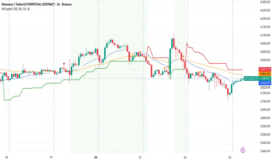
Hello Crypto! Modern Combo Snapshot
Unified long/short analyzer blending EMA structure, SuperTrend, WaveTrend, QQE, and volume pressure.
Background shading flags “watch” and “ready” states; optional long/short modules let you focus on one side.
Alerts fire when every checklist item aligns, while the side-panel table summarizes trend, momentum, liquidity, and overall score in real time.
Indicator → Trend Analysis
Indicator → Momentum Oscillators
Indicator → Volume Indicators
Tags:
cryptocurrency, bitcoin, altcoins, trend-following, momentum, volume, ema, supertrend, intraday, swing-trading, alerts, checklist, trading-strategy, risk-management
Modern Combo Crypto SuiteBlends long and short playbooks in one overlay with quick toggles.
Tracks EMA stacks, SuperTrend, WaveTrend, QQE, and volume to score bias.
Colors the chart background when watch/ready conditions align.
Fires alerts for imminent or fully aligned long/short setups.
Displays a live checklist table summarizing trend, momentum, and volume confidence.

Cycle VTLs – with Scaled Channels "Cycle VTLs – with Scaled Channels" for TradingView plots Valid Trend Lines (VTLs) based on Hurst's Cyclic Theory, connecting consecutive price peaks (downward VTLs) or troughs (upward VTLs) for specific cycles. It uses up to eight Simple Moving Averages (SMAs) (default lengths: 25, 50, 100, 200, 400, 800, 1600, 1600 bars) with customizable envelope bands to detect pivots and draw VTLs, enhanced by optional parallel channels scaled to envelope widths.
Key Features:
Valid Trend Lines (VTLs):
Upward VTLs: Connect consecutive cycle troughs, sloping upward.
Downward VTLs: Connect consecutive cycle peaks, sloping downward.
Hurst’s Rules:
Connects consecutive cycle peaks/troughs.
Must not cross price between points.
Downward VTLs:
No longer-cycle trough between peaks.
Invalid if slope is incorrect (upward VTL not up, downward VTL not down).
Expired VTLs: Historical VTLs (crossed by price) from up to three prior cycle waves.
SMA Cycles:
Eight customizable SMAs with envelope bands (offset × multiplier) for pivot detection.
Channels:
Optional parallel lines around VTLs, width set by channelFactor × envelope half-width.
Pivot Detection:
Fractal-based (pivotPeriod) on envelopes or price (usePriceFallback).
Customization:
Toggle cycles, VTLs, and channels.
Adjust SMA lengths, offsets, colors, line styles, and widths.
Enable centered envelopes, slope filtering, and limit stored lines (maxStoredLines).
Usage in Hurst’s Cyclic TheoryAnalysis:
VTLs identify cycle trends; upward VTLs suggest bullish momentum, downward VTLs bearish.
Price crossing below an upward VTL confirms a peak in the next longer cycle; crossing above a downward VTL confirms a trough.
Trading:
Buy: Price bounces off upward VTL or breaks above downward VTL.
Sell: Price rejects downward VTL or breaks below upward VTL.
Use channels for support/resistance, breakouts, or stop-loss/take-profit levels.
Workflow:
Add indicator on TradingView.
Enable desired cycles (e.g., 50-bar, 1600-bar), adjust pivotPeriod, channelFactor, and showOnlyCorrectSlope.
Monitor VTL crossings and channels for trade signals.
NotesOptimized for performance with line limits.
Ideal for cycle-based trend analysis across markets (stocks, forex, crypto).
Debug labels show pivot counts and VTL status.
This indicator supports Hurst’s Cyclic Theory for trend identification and trading decisions with flexible, cycle-based VTLs and channels.
Use global variable to scale to chart. best results use factors of 2 and double. try 2, 4, 8, 16...128, 256, etc until price action fits 95% in smallest cycle.
Pro Momentum Table + Trade Alerts📊 Indicator Name: Pro Momentum Table – ADX + DI + ATR + Astro Timing
🧠 Concept:
This indicator is designed for professional scalpers and intraday traders who want to capture only strong momentum waves — not noise. It combines trend strength, volatility, directional movement, momentum oscillation, vega divergence, and astrological timing into a single compact table on your chart.
⚙️ Components Explained:
Metric Description
ADX (Average Directional Index) Measures the strength of the trend. Values above 20 indicate that a meaningful move is starting.
+DI / -DI (Directional Indicators) Show whether buyers (+DI) or sellers (-DI) are dominating. Increasing +DI with ADX rising = bullish momentum. Increasing -DI with ADX rising = bearish momentum.
ATR (Average True Range) Shows volatility and expected range. Used for setting realistic stop-loss and multi-level targets (1×, 1.5×, 2×, 2.5× ATR).
Price Displays the current price level for quick reference.
CMO (Chande Momentum Oscillator) Measures short-term momentum direction and strength. Helps identify overbought/oversold conditions in trend continuation.
Vega Divergence Shows a synthetic reading of volatility pressure — "Bullish" when volatility expansion supports upward moves, "Bearish" for downward pressure, and "Neutral" otherwise.
Astro Remark Suggests ideal time windows based on planetary cycles for scalping entries. “Bullish Window” often aligns with high-probability long trades; “Bearish Window” favors shorts.
Trade Signal The core momentum condition: “Bullish Momentum” if ADX > 20 and +DI rising, “Bearish Momentum” if ADX > 20 and -DI rising, else “No Clear Momentum.”
📈 How to Use:
Wait for ADX > 20 – This confirms that the market is entering a strong momentum phase.
Check DI direction:
✅ +DI rising: Buyers gaining strength → look for long setups.
✅ -DI rising: Sellers gaining strength → look for short setups.
Use ATR to plan exits:
🎯 TP1 = Entry ± 1 × ATR
🎯 TP2 = Entry ± 1.5 × ATR
🎯 TP3 = Entry ± 2 × ATR
🎯 TP4 = Entry ± 2.5 × ATR
CMO & Vega Divergence: Confirm momentum direction and volatility expansion before committing.
Astro Remark: Align your scalping activity with the planetary support window for higher probability trades.
🪙 Pro Tips for Scalpers:
Only trade when ADX > 20 and DI is consistently rising. Ignore signals in choppy or sideways phases.
Avoid trades if Vega is neutral and CMO is flat – these usually indicate fake breakouts.
If targets aren’t hit within expected ATR-based time, treat the move as false and exit early.
Combine with 9 EMA and 20 EMA (hidden) for wave structure confirmation without cluttering the chart.
💡 Summary:
This indicator acts as a real-time trade decision dashboard. It removes clutter from the chart and delivers everything a professional scalper needs — strength, direction, volatility, momentum, timing, and actionable trade bias — all in one elegant table.
