Crypto McClellan Oscillator (SLN Fix)This is an adaption of the Mcclellan Oscillator for crypto. Instead of tracking the S&P500 it tracks a selection of cryptos to make sure the indicator follows this sector instead.
Full credit goes to the creator of this indicator: Fadior. It has since been fixed by SLN.
The following description explains the standard McClellan Oscillator. Full credit to Investopedia , my fav source of financial explanations.
The same principles applies to its use in the crypto sector, but please be cautious of the last point, the limitations. Since crypto is more volatile, that could amplify choppy behavior.
This is not financial advice, please be extremely cautious. This indicator is only suitable as a confirmation signal and needs support of other signals to be profitable.
This indicator usually produces the best signals on slightly above daily time frame. I personally like 2 or 3 day, but you have to find the settings suitable for your trading style.
What Is the McClellan Oscillator?
The McClellan Oscillator is a market breadth indicator that is based on the difference between the number of advancing and declining issues on a stock exchange, such as the New York Stock Exchange (NYSE) or NASDAQ.
The indicator is used to show strong shifts in sentiment in the indexes, called breadth thrusts. It also helps in analyzing the strength of an index trend via divergence or confirmation.
The McClellan Oscillator formula can be applied to any stock exchange or group of stocks.
A reading above zero helps confirm a rise in the index, while readings below zero confirm a decline in the index.
When the index is rising but the oscillator is falling, that warns that the index could start declining too. When the index is falling and the oscillator is rising, that indicates the index could start rising soon. This is called divergence.
A significant change, such as moving 100 points or more, from a negative reading to a positive reading is called a breadth thrust. It may indicate a strong reversal from downtrend to uptrend is underway on the stock exchange.
How to Calculate the McClellan Oscillator
To get the calculation started, track Advances - Declines on a stock exchange for 19 and 39 days. Calculate a simple average for these, not exponential moving average (EMA).
Use these simple values as the Prior Day EMA values in the 19- and 39-day EMA formulas.
Calculate the 19- and 39-day EMAs.
Calculate the McClellan Oscillator value.
Now that the value has been calculated, on the next calculation use this value for the Prior Day EMA. Start calculating EMAs for the formula instead of simple averages.
If using the adjusted formula, the steps are the same, except use ANA instead of using Advances - Declines.
What Does the McClellan Oscillator Tell You?
The McClellan Oscillator is an indicator based on market breadth which technical analysts can use in conjunction with other technical tools to determine the overall state of the stock market and assess the strength of its current trend.
Since the indicator is based on all the stocks in an exchange, it is compared to the price movements of indexes that reflect that exchange, or compared to major indexes such as the S&P 500.
Positive and negative values indicate whether more stocks, on average, are advancing or declining. The indicator is positive when the 19-day EMA is above the 39-day EMA, and negative when the 19-day EMA is below the 39-day EMA.
A positive and rising indicator suggests that stocks on the exchange are being accumulated. A negative and falling indicator signals that stocks are being sold. Typically such action confirms the current trend in the index.
Crossovers from positive to negative, or vice versa, may signal the trend has changed in the index or exchange being tracked. When the indicator makes a large move, typically of 100 points or more, from negative to positive territory, that is called a breadth thrust.
It means a large number of stocks moved up after a bearish move. Since the stock market tends to rise over time, this a positive signal and may indicate that a bottom in the index is in and prices are heading higher overall.
When index prices and the indicator are moving in different directions, then the current index trend may lack strength. Bullish divergence occurs when the oscillator is rising while the index is falling. This indicates the index could head higher soon since more stocks are starting to advance.
Bearish divergence is when the index is rising and the indicator is falling. This means fewer stocks are keeping the advance going and prices may start to head lower.
Limitations of Using the McClellan Oscillator
The indicator tends to produce lots of signals. Breadth thrusts, divergence, and crossovers all occur with some frequency, but not all these signals will result in the price/index moving in the expected direction.
The indicator is prone to producing false signals and therefore should be used in conjunction with price action analysis and other technical indicators.
The indicator can also be quite choppy, moving between positive and negative territory rapidly. Such action indicates a choppy market, but this isn't evident until the indicator has made this whipsaw move a few times.
Good luck and a big thanks to Fadior!
Cari dalam skrip untuk "初中数学动点最值问题19大模型+例题详解"

Pre-COVID High and COVID LowOverview
The "Pre-COVID High and COVID Low" indicator is designed to identify and mark significant price levels on your chart, specifically targeting the pre-COVID-19 high and the low during the initial COVID-19 market impact. This script is particularly useful for traders who are interested in analyzing how stocks or other financial instruments reacted during the onset of the COVID-19 pandemic, providing a historical perspective that may help in making informed trading decisions.
How It Works
Date Ranges : The script uses predefined date ranges to calculate the highest and lowest price levels before and during the early stages of the COVID-19 pandemic. These ranges are:
Pre-COVID High: Between January 1, 2020, and March 31, 2020.
COVID Low: Between March 1, 2020, and March 31, 2020.
Calculation Method :
The highest price during the pre-COVID period is tracked and recorded as the "Pre-COVID High".
The lowest price during the specified COVID period is tracked and recorded as the "COVID Low".
Visibility Conditions : The script includes logic to ensure that these historical levels are only displayed if they fall within a range close to the current visible price range on the chart. This prevents the indicator from compressing the price scale unduly.
How to Use It
Adding to Your Char t: To use this indicator, add it to any chart on TradingView. It works best with daily time frames to clearly visualize the impact over these specific months.
Interpretation :
The "Pre-COVID High" is marked with a red line and is labeled the first day it becomes applicable.
The "COVID Low" is marked with a green line and is similarly labeled on its applicable day.
Trading Strategy Consideration : Traders can use these historical levels as potential support or resistance zones for their trading strategies. These levels can indicate significant price points where the market previously showed strong reactions.

Baha'i Reversal Points [CC]The Baha'i Reversal Points is a custom creation that combines some of my favorite passions, creating stock indicator scripts and my faith. The Baha'i Faith believes in the oneness of God and all religions, and sees the number 9 as significant because that is the number of major world religions as well as the Baha'i symbol is a nine-pointed star. The number 19 is also seen as significant because in the Baha'i calendar, there are 19 months, and each month is made up of 19 days. Anyway, with all that being explained, I created these reversal points to find the points where the last 19 highs or lows are higher or lower, respectively than the previous high or low nine days ago. As with many indicators, this does have some hits and misses but does a pretty good job of finding reversal points based on these criteria.
There are a few different ways to analyze this data to determine when to buy or sell. I have set the default behavior for when we encounter the first time that the amount of highs or lows is greater than or equal to the length amount using a crossover or crossunder alert. You could also ignore the crossover or crossunder alerts and buy when the count is greater than or equal to the length, which can happen for extended periods depending on the underlying trend. Overall, buy when the buy label appears and sell when the sell label appears.
Let me know if there are any other custom indicators or scripts you would like to see me publish!

TARVIS Labs - Bitcoin Macro Bottom/Top SignalsSCRIPT DESCRIPTION
This is a script specifically written to help provide indicators from a macro view. This script is best run on the 1 day interval on Bitstamp's $BTCUSD chart. It helps indicate when to accumulate bitcoin, and when its in a bull run when there are local tops, strong top warnings, and a signal to exit a bull run. This is described further below.
If you don't have interest in trading on the way to the top I suggest turning off the following indicators in the settings of the indicator:
- Opportunity To Buy Back In Indicator
- Local Top Near Bull Run Top Indicator
ACCUMULATION ZONE INDICATOR - LIGHT GREEN
Description
When we look at the history of Bitcoin every bottom has crossed below the 100 week EMA. Once it does its accompanied by hash ribbon cross with miner capitulation. After that is the prime time to accumulate as theres a clearer signal the bottom is in. Specifically, a signal to look for is the 14 day MACD/signal cross and the 14 day MACD continuing to stay above the signal until the price returns above the 100 week EMA. This is prime accumulation territory.
Strategy for Usage
A good strategy to use when accumulating the bottom is dollar-cost averaging over a 30 day period. The accumulation zone can last longer than 30 days but 30 days is a good range of time to DCA.
STRONG BUY IN ACCUMULATION ZONE INDICATOR - DARK GREEN
Description
We can add to the bottoming signal by looking for post-downtrend reversals inside the bottoming signal. We do this by using a 9/19 daily cross.
Strategy for Usage
These post-downtrend reversals can potentially provide better targeted days for accumulation than the broader bottoming signal and can be used to add more on that day than on an average day for the dollar cost average strategy. Say for example, use 1/3 of funds on these days rather than 1/30th.
OPPORTUNITY TO BUY BACK IN INDICATOR - BLUE
Description
When the 1d 18 EMA > 1d 63 EMA and the 12/52 1d crosses. These together provide good buy opportunities to buy bitcoin.
Strategy for Usage
If you happen to find yourself out of the market from your own TA or a trade, this signal can provide a buy opportunity to reenter the market if you're out of it.
BULL RUN LOCAL TOP INDICATOR - ORANGE
Description
We will similarly use the 100 week EMA to determine trend reversal into a bull run. When we see the 100 week EMA uptrending, we can begin to look for local tops using the 9/19 daily MACD/signal bearish cross along with the 12 EMA having a negative slope, which could be the beginning signal for a local top.
Strategy for Usage
This is a rather light indicator, but can be used in tandem with your own technical analysis to determine if you want to reenter after you exit from its signal.
LOCAL TOP NEAR BULL RUN TOP INDICATOR - RED
Description
When the 100 week EMA is in an uptrend we can look for significant loss of momentum in order to determine if a local top is in near a bull run top. Similar to the Bull Run Local Top Indicator, this strategy uses a MACD/signal cross but instead uses the 30/65 day EMAs.
Strategy for Usage
Ideally the right strategy to use here is to exit the market when this indicator starts. When the indicator ends if the "End of Bull Run Indicator" is not showing on the chart you can buy back into the market.
TOP IS LIKELY IN INDICATOR
Description
When the 100 week EMA is in a very strong uptrend and the 9/19 weekly MACD/signal bearish cross occurs, and the 63 EMA begins to downtrend.
Strategy for Usage
This signal typically accompanies the "Local Top Near Bull Run Top Indicator" therefore if you're following the strategy you would likely already be out of the market, but if you're not and this signal fires its a strong signal the top is in and we're likely going to start seeing a strong retrace. This is typically right before we see the "End of Bull Run Indicator". There is only one occurrence where it wasn't followed by a large drop & the "End of Bull Run Indicator" and that was in the 2017 bull run where there were many strong retracements post local top. The likelihood we see that again is low, but if it were to happen you can buy back into the market when the "Top is Likely In Indicator" and the "Local Top Near Bull Run Top Indicator" are not firing.
TOP IS LIKELY IN INDICATOR
Description
When the 100 week EMA is in a strong uptrend and the 9/19 weekly MACD/signal bearish cross occurs, and the 63 EMA begins to downtrend.
Strategy for Usage
This signal typically accompanies the "Local Top Near Bull Run Top Indicator" therefore if you're following the strategy you would likely already be out of the market, but if you're not and this signal fires its a strong signal the top is in and we're likely going to start seeing a strong retrace. This is typically right before we see the "End of Bull Run Indicator". There is only one occurrence where it wasn't followed by a large drop & the "End of Bull Run Indicator" and that was in the 2017 bull run where there were many strong retracements post local top. The likelihood we see that again is low, but if it were to happen you can buy back into the market when the "Top is Likely In Indicator" and the "Local Top Near Bull Run Top Indicator" are not firing.
END OF BULL RUN INDICATOR
Description
When the 100 week EMA is in an uptrend and the 1d 18 EMA crosses the 1d 63 EMA.
Strategy for Usage
When the 100 week EMA is a strong uptrend and the 18/63 cross occurs the top is very likely in. It has occurred in every bull run top leading to the bear market.

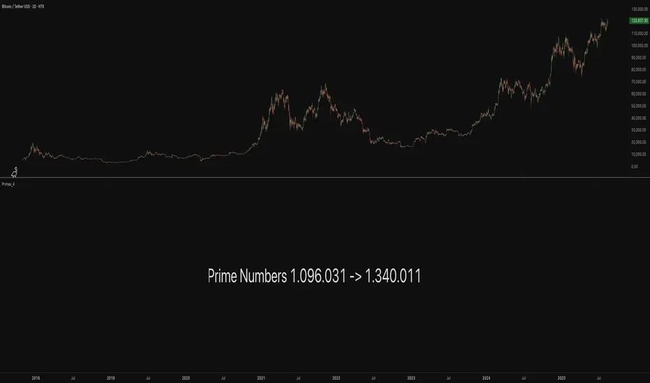
Primes_4These libraries (Primes_1 -> Primes_4) contain arrays of reduced Prime Numbers to minimize the amount of tokens, allowing more information to be exported.
Values, for example:
7001, 7013, 7019, 7027, 7039, 7043, 7057, 7069, 7079, 7103, 7109, 7021
are reduced to:
7001, 13, 19, 27, 39, 43, 57, 69, 79, 7103, 9, 21
With the restoreValues() function found in this library, the reduced values can be restored back to its original state.
7001, 13, 19, 27, 39, 43, 57, 69, 79, 7103, 9, 21
is restored back to:
7001, 7013, 7019, 7027, 7039, 7043, 7057, 7069, 7079, 7103, 7109, 7021
The libraries contain all Prime Numbers from 2 to 1.340.011
------------------------------------------------------------
Library "Primes_4"
Prime Numbers 1.096.031 - 1.340.011
primes_a()
Prime numbers 1.096.031 - 1.205.999
primes_b()
Prime numbers 1.206.013 - 1.317.989
primes_c()
Prime numbers 1.318.003 - 1.340.011
method restoreValues(iArray, iShow, iFrom, iTo)
restoreValues : Restores reduced prime number values in an array to their original state, for example `7001, 13, 19, 27, 39, 43, 57, 69, 79, 7103, 9, 21` is restored to `7001, 7013, 7019, 7027, 7039, 7043, 7057, 7069, 7079, 7103, 7109, 7021`
Namespace types: array
Parameters:
iArray (array)
iShow (bool)
iFrom (int)
iTo (int)
Returns: Initial array with restored prime number values
Ratio-Adjusted McClellan Summation Index RASI NASIRatio-Adjusted McClellan Summation Index (RASI NASI)
In Book "The Complete Guide to Market Breadth Indicators" Author Gregory L. Morris states
"It is the author’s opinion that the McClellan indicators, and in particular, the McClellan Summation Index, is the single best breadth indicator available. If you had to pick just one, this would be it."
What It Does: The Ratio-Adjusted McClellan Summation Index (RASI) is a market breadth indicator that tracks the cumulative strength of advancing versus declining issues for a user-selected exchange (NASDAQ, NYSE, or AMEX). Derived from the McClellan Oscillator, it calculates ratio-adjusted net advances, applies 19-day and 39-day EMAs, and sums the oscillator values to produce the RASI. This indicator helps traders assess market health, identify bullish or bearish trends, and detect potential reversals through divergences.
Key features:
Exchange Selection : Choose NASDAQ (USI:ADVN.NQ, USI:DECL.NQ), NYSE (USI:ADVN.NY, USI:DECL.NY), or AMEX (USI:ADVN.AM, USI:DECL.AM) data.
Trend-Based Coloring : RASI line displays user-defined colors (default: black for uptrend, red for downtrend) based on its direction.
Customizable Moving Average: Add a moving average (SMA, EMA, WMA, VWMA, or RMA) with user-defined length and color (default: EMA, 21, green).
Neutral Line at Zero: Marks the neutral level for trend interpretation.
Alerts: Six custom alert conditions for trend changes, MA crosses, and zero-line crosses.
How to Use
Add to Chart: Apply the indicator to any TradingView chart. Ensure access to advancing and declining issues data for the selected exchange.
Select Exchange: Choose NASDAQ, NYSE, or AMEX in the input settings.
Customize Settings: Adjust EMA lengths, RASI colors, MA type, length, and color to match your trading style.
Interpret the Indicator :
RASI Line: Black (default) indicates an uptrend (RASI rising); red indicates a downtrend (RASI falling).
Above Zero: Suggests bullish market breadth (more advancing issues).
Below Zero : Indicates bearish breadth (more declining issues).
MA Crosses: RASI crossing above its MA signals bullish momentum; crossing below signals bearish momentum.
Divergences: Compare RASI with the market index (e.g., NASDAQ Composite) to identify potential reversals.
Large Moves : A +3,600-point move from a low (e.g., -1,550 to +1,950) may signal a significant bull run.
Set Alerts:
Add the indicator to your chart, open the TradingView alert panel, and select from six conditions (see Alerts section).
Configure notifications (e.g., email, webhook, or popup) for each condition.
Settings
Market Selection:
Exchange: Select NASDAQ, NYSE, or AMEX for advancing/declining issues data.
EMA Settings:
19-day EMA Length: Period for the shorter EMA (default: 19).
39-day EMA Length: Period for the longer EMA (default: 39).
RASI Settings:
RASI Uptrend Color: Color for rising RASI (default: black).
RASI Downtrend Color: Color for falling RASI (default: red).
RASI MA Settings:
MA Type: Choose SMA, EMA, WMA, VWMA, or RMA (default: EMA).
MA Length: Set the MA period (default: 21).
MA Color: Color for the MA line (default: green).
Alerts
The indicator uses alertcondition() to create custom alerts. Available conditions:
RASI Trend Up: RASI starts rising (based on RASI > previous RASI, shown as black line).
RASI Trend Down: RASI starts falling (based on RASI ≤ previous RASI, shown as red line).
RASI Above MA: RASI crosses above its moving average.
RASI Below MA: RASI crosses below its moving average.
RASI Bullish: RASI crosses above zero (bullish market breadth).
RASI Bearish: RASI crosses below zero (bearish market breadth).
To set alerts, add the indicator to your chart, open the TradingView alert panel, and select the desired condition.
Notes
Data Requirements: Requires access to advancing/declining issues data (e.g., USI:ADVN.NQ, USI:DECL.NQ for NASDAQ). Some symbols may require a TradingView premium subscription.
Limitations: RASI is a medium- to long-term indicator and may lag in volatile or range-bound markets. Use alongside other technical tools for confirmation.
Data Reliability : Verify the selected exchange’s data accuracy, as inconsistencies can affect results.
Debugging: If no data appears, check symbol validity (e.g., try $ADVN/Q, $DECN/Q for NASDAQ) or contact TradingView support.
Credits
Based on the Ratio-Adjusted McClellan Summation Index methodology by McClellan Financial Publications. No external code was used; the implementation is original, inspired by standard market breadth concepts.
Disclaimer
This indicator is for informational purposes only and does not constitute financial advice. Past performance is not indicative of future results. Conduct your own research and combine with other tools for informed trading decisions.

Multi-Session ORBThe Multi-Session ORB Indicator is a customizable Pine Script (version 6) tool designed for TradingView to plot Opening Range Breakout (ORB) levels across four major trading sessions: Sydney, Tokyo, London, and New York. It allows traders to define specific ORB durations and session times in Central Daylight Time (CDT), making it adaptable to various trading strategies.
Key Features:
1. Customizable ORB Duration: Users can set the ORB duration (default: 15 minutes) via the inputMax parameter, determining the time window for calculating the high and low of each session’s opening range.
2. Flexible Session Times: The indicator supports user-defined session and ORB times for:
◦ Sydney: Default ORB (17:00–17:15 CDT), Session (17:00–01:00 CDT)
◦ Tokyo: Default ORB (19:00–19:15 CDT), Session (19:00–04:00 CDT)
◦ London: Default ORB (02:00–02:15 CDT), Session (02:00–11:00 CDT)
◦ New York: Default ORB (08:30–08:45 CDT), Session (08:30–16:00 CDT)
3. Session-Specific ORB Levels: For each session, the indicator calculates and tracks the high and low prices during the specified ORB period. These levels are updated dynamically if new highs or lows occur within the ORB timeframe.
4. Visual Representation:
◦ ORB high and low lines are plotted only during their respective session times, ensuring clarity.
◦ Each session’s lines are color-coded for easy identification:
▪ Sydney: Light Yellow (high), Dark Yellow (low)
▪ Tokyo: Light Pink (high), Dark Pink (low)
▪ London: Light Blue (high), Dark Blue (low)
▪ New York: Light Purple (high), Dark Purple (low)
◦ Lines are drawn with a linewidth of 2 and disappear when the session ends or if the timeframe is not intraday (or exceeds the ORB duration).
5. Intraday Compatibility: The indicator is optimized for intraday timeframes (e.g., 1-minute to 15-minute charts) and only displays when the chart’s timeframe multiplier is less than or equal to the ORB duration.
How It Works:
• Session Detection: The script uses the time() function to check if the current bar falls within the user-defined ORB or session time windows, accounting for all days of the week.
• ORB Logic: At the start of each session’s ORB period, the script initializes the high and low based on the first bar’s prices. It then updates these levels if subsequent bars within the ORB period exceed the current high or fall below the current low.
• Plotting: ORB levels are plotted as horizontal lines during the respective session, with visibility controlled to avoid clutter outside session times or on incompatible timeframes.
Use Case:
Traders can use this indicator to identify key breakout levels for each trading session, facilitating strategies based on price action around the opening range. The flexibility to adjust ORB and session times makes it suitable for various markets (e.g., forex, stocks, or futures) and time zones.
Limitations:
• The indicator is designed for intraday timeframes and may not display on higher timeframes (e.g., daily or weekly) or if the timeframe multiplier exceeds the ORB duration.
• Time inputs are in CDT, requiring users to adjust for their local timezone or market requirements.
• If you need to use this for GC/CL/SPY/QQQ you have to adjust the times by one hour.
This indicator is ideal for traders focusing on session-based breakout strategies, offering clear visualization and customization for global market sessions.

[GYTS] FiltersToolkit LibraryFiltersToolkit Library
🌸 Part of GoemonYae Trading System (GYTS) 🌸
🌸 --------- 1. INTRODUCTION --------- 🌸
💮 What Does This Library Contain?
This library is a curated collection of high-performance digital signal processing (DSP) filters and auxiliary functions designed specifically for financial time series analysis. It includes a shortlist of our favourite and best performing filters — each rigorously tested and selected for their responsiveness, minimal lag and robustness in diverse market conditions. These tools form an integral part of the GoemonYae Trading System (GYTS), chosen for their unique characteristics in handling market data.
The library contains two main categories:
1. Smoothing filters (low-pass filters and moving averages) for e.g. denoising, trend following
2. Detrending tools (high-pass and band-pass filters, known as "oscillators") for e.g. mean reversion
This collection is finely tuned for practical trading applications and is therefore not meant to be exhaustive. However, will continue to expand as we discover and validate new filtering techniques. I welcome collaboration and suggestions for novel approaches.
🌸 ——— 2. ADDED VALUE ——— 🌸
💮 Unified syntax and comprehensive documentation
The FiltersToolkit Library brings together a wide array of valuable filters under a unified, intuitive syntax. Each function is thoroughly documented, with clear explanations and academic sources that underline the mathematical rigour behind the methods. This level of documentation not only facilitates integration into trading strategies but also helps underlying the underlying concepts and rationale.
💮 Optimised performance and readability
The code prioritizes computational efficiency while maintaining readability. Key optimizations include:
- Minimizing redundant calculations in recursive filters
- Smart coefficient caching
- Efficient state management
- Vectorized operations where applicable
💮 Enhanced functionality and flexibility
Some filters in this library introduce extended functionality beyond the original publications. For instance, the MESA Adaptive Moving Average (MAMA) and Ehlers’ Combined Bandpass Filter incorporate multiple variations found in the literature, thereby providing traders with flexible tools that can be fine-tuned to different market conditions.
🌸 ——— 3. THE FILTERS ——— 🌸
💮 Hilbert Transform Function
This function implements the Hilbert Transform as utilised by John Ehlers. It converts a real-valued time series into its analytic signal, enabling the extraction of instantaneous phase and frequency information—an essential step in adaptive filtering.
Source: John Ehlers - "Rocket Science for Traders" (2001), "TASC 2001 V. 19:9", "Cybernetic Analysis for Stocks and Futures" (2004)
💮 Homodyne Discriminator
By leveraging the Hilbert Transform, this function computes the dominant cycle period through a Homodyne Discriminator. It extracts the in-phase and quadrature components of the signal, facilitating a robust estimation of the underlying cycle characteristics.
Source: John Ehlers - "Rocket Science for Traders" (2001), "TASC 2001 V. 19:9", "Cybernetic Analysis for Stocks and Futures" (2004)
💮 MESA Adaptive Moving Average (MAMA)
An advanced dual-stage adaptive moving average, this function outputs both the MAMA and its companion FAMA. It combines adaptive alpha computation with elements from Kaufman’s Adaptive Moving Average (KAMA) to provide a responsive and reliable trend indicator.
Source: John Ehlers - "Rocket Science for Traders" (2001), "TASC 2001 V. 19:9", "Cybernetic Analysis for Stocks and Futures" (2004)
💮 BiQuad Filters
A family of second-order recursive filters offering exceptional control over frequency response:
- High-pass filter for detrending
- Low-pass filter for smooth trend following
- Band-pass filter for cycle isolation
The quality factor (Q) parameter allows fine-tuning of the resonance characteristics, making these filters highly adaptable to different market conditions.
Source: Robert Bristow-Johnson's Audio EQ Cookbook, implemented by @The_Peaceful_Lizard
💮 Relative Vigor Index (RVI)
This filter evaluates the strength of a trend by comparing the closing price to the trading range. Operating similarly to a band-pass filter, the RVI provides insights into market momentum and potential reversals.
Source: John Ehlers – “Cybernetic Analysis for Stocks and Futures” (2004)
💮 Cyber Cycle
The Cyber Cycle filter emphasises market cycles by smoothing out noise and highlighting the dominant cyclical behaviour. It is particularly useful for detecting trend reversals and cyclical patterns in the price data.
Source: John Ehlers – “Cybernetic Analysis for Stocks and Futures” (2004)
💮 Butterworth High Pass Filter
Inspired by the classical Butterworth design, this filter achieves a maximally flat magnitude response in the passband while effectively removing low-frequency trends. Its design minimises phase distortion, which is vital for accurate signal interpretation.
Source: John Ehlers – “Cybernetic Analysis for Stocks and Futures” (2004)
💮 2-Pole SuperSmoother
Employing a two-pole design, the SuperSmoother filter reduces high-frequency noise with minimal lag. It is engineered to preserve trend integrity while offering a smooth output even in noisy market conditions.
Source: John Ehlers – “Cybernetic Analysis for Stocks and Futures” (2004)
💮 3-Pole SuperSmoother
An extension of the 2-pole design, the 3-pole SuperSmoother further attenuates high-frequency noise. Its additional pole delivers enhanced smoothing at the cost of slightly increased lag.
Source: John Ehlers – “Cybernetic Analysis for Stocks and Futures” (2004)
💮 Adaptive Directional Volatility Moving Average (ADXVma)
This adaptive moving average adjusts its smoothing factor based on directional volatility. By combining true range and directional movement measurements, it remains exceptionally flat during ranging markets and responsive during directional moves.
Source: Various implementations across platforms, unified and optimized
💮 Ehlers Combined Bandpass Filter with Automated Gain Control (AGC)
This sophisticated filter merges a highpass pre-processing stage with a bandpass filter. An integrated Automated Gain Control normalises the output to a consistent range, while offering both regular and truncated recursive formulations to manage lag.
Source: John F. Ehlers – “Truncated Indicators” (2020), “Cycle Analytics for Traders” (2013)
💮 Voss Predictive Filter
A forward-looking filter that predicts future values of a band-limited signal in real time. By utilising multiple time-delayed feedback terms, it provides anticipatory coupling and delivers a short-term predictive signal.
Source: John Ehlers - "A Peek Into The Future" (TASC 2019-08)
💮 Adaptive Autonomous Recursive Moving Average (A2RMA)
This filter dynamically adjusts its smoothing through an adaptive mechanism based on an efficiency ratio and a dynamic threshold. A double application of an adaptive moving average ensures both responsiveness and stability in volatile and ranging markets alike. Very flat response when properly tuned.
Source: @alexgrover (2019)
💮 Ultimate Smoother (2-Pole)
The Ultimate Smoother filter is engineered to achieve near-zero lag in its passband by subtracting a high-pass response from an all-pass response. This creates a filter that maintains signal fidelity at low frequencies while effectively filtering higher frequencies at the expense of slight overshooting.
Source: John Ehlers - TASC 2024-04 "The Ultimate Smoother"
Note: This library is actively maintained and enhanced. Suggestions for additional filters or improvements are welcome through the usual channels. The source code contains a list of tested filters that did not make it into the curated collection.
Universal Ratio Trend Matrix [InvestorUnknown]The Universal Ratio Trend Matrix is designed for trend analysis on asset/asset ratios, supporting up to 40 different assets. Its primary purpose is to help identify which assets are outperforming others within a selection, providing a broad overview of market trends through a matrix of ratios. The indicator automatically expands the matrix based on the number of assets chosen, simplifying the process of comparing multiple assets in terms of performance.
Key features include the ability to choose from a narrow selection of indicators to perform the ratio trend analysis, allowing users to apply well-defined metrics to their comparison.
Drawback: Due to the computational intensity involved in calculating ratios across many assets, the indicator has a limitation related to loading speed. TradingView has time limits for calculations, and for users on the basic (free) plan, this could result in frequent errors due to exceeded time limits. To use the indicator effectively, users with any paid plans should run it on timeframes higher than 8h (the lowest timeframe on which it managed to load with 40 assets), as lower timeframes may not reliably load.
Indicators:
RSI_raw: Simple function to calculate the Relative Strength Index (RSI) of a source (asset price).
RSI_sma: Calculates RSI followed by a Simple Moving Average (SMA).
RSI_ema: Calculates RSI followed by an Exponential Moving Average (EMA).
CCI: Calculates the Commodity Channel Index (CCI).
Fisher: Implements the Fisher Transform to normalize prices.
Utility Functions:
f_remove_exchange_name: Strips the exchange name from asset tickers (e.g., "INDEX:BTCUSD" to "BTCUSD").
f_remove_exchange_name(simple string name) =>
string parts = str.split(name, ":")
string result = array.size(parts) > 1 ? array.get(parts, 1) : name
result
f_get_price: Retrieves the closing price of a given asset ticker using request.security().
f_constant_src: Checks if the source data is constant by comparing multiple consecutive values.
Inputs:
General settings allow users to select the number of tickers for analysis (used_assets) and choose the trend indicator (RSI, CCI, Fisher, etc.).
Table settings customize how trend scores are displayed in terms of text size, header visibility, highlighting options, and top-performing asset identification.
The script includes inputs for up to 40 assets, allowing the user to select various cryptocurrencies (e.g., BTCUSD, ETHUSD, SOLUSD) or other assets for trend analysis.
Price Arrays:
Price values for each asset are stored in variables (price_a1 to price_a40) initialized as na. These prices are updated only for the number of assets specified by the user (used_assets).
Trend scores for each asset are stored in separate arrays
// declare price variables as "na"
var float price_a1 = na, var float price_a2 = na, var float price_a3 = na, var float price_a4 = na, var float price_a5 = na
var float price_a6 = na, var float price_a7 = na, var float price_a8 = na, var float price_a9 = na, var float price_a10 = na
var float price_a11 = na, var float price_a12 = na, var float price_a13 = na, var float price_a14 = na, var float price_a15 = na
var float price_a16 = na, var float price_a17 = na, var float price_a18 = na, var float price_a19 = na, var float price_a20 = na
var float price_a21 = na, var float price_a22 = na, var float price_a23 = na, var float price_a24 = na, var float price_a25 = na
var float price_a26 = na, var float price_a27 = na, var float price_a28 = na, var float price_a29 = na, var float price_a30 = na
var float price_a31 = na, var float price_a32 = na, var float price_a33 = na, var float price_a34 = na, var float price_a35 = na
var float price_a36 = na, var float price_a37 = na, var float price_a38 = na, var float price_a39 = na, var float price_a40 = na
// create "empty" arrays to store trend scores
var a1_array = array.new_int(40, 0), var a2_array = array.new_int(40, 0), var a3_array = array.new_int(40, 0), var a4_array = array.new_int(40, 0)
var a5_array = array.new_int(40, 0), var a6_array = array.new_int(40, 0), var a7_array = array.new_int(40, 0), var a8_array = array.new_int(40, 0)
var a9_array = array.new_int(40, 0), var a10_array = array.new_int(40, 0), var a11_array = array.new_int(40, 0), var a12_array = array.new_int(40, 0)
var a13_array = array.new_int(40, 0), var a14_array = array.new_int(40, 0), var a15_array = array.new_int(40, 0), var a16_array = array.new_int(40, 0)
var a17_array = array.new_int(40, 0), var a18_array = array.new_int(40, 0), var a19_array = array.new_int(40, 0), var a20_array = array.new_int(40, 0)
var a21_array = array.new_int(40, 0), var a22_array = array.new_int(40, 0), var a23_array = array.new_int(40, 0), var a24_array = array.new_int(40, 0)
var a25_array = array.new_int(40, 0), var a26_array = array.new_int(40, 0), var a27_array = array.new_int(40, 0), var a28_array = array.new_int(40, 0)
var a29_array = array.new_int(40, 0), var a30_array = array.new_int(40, 0), var a31_array = array.new_int(40, 0), var a32_array = array.new_int(40, 0)
var a33_array = array.new_int(40, 0), var a34_array = array.new_int(40, 0), var a35_array = array.new_int(40, 0), var a36_array = array.new_int(40, 0)
var a37_array = array.new_int(40, 0), var a38_array = array.new_int(40, 0), var a39_array = array.new_int(40, 0), var a40_array = array.new_int(40, 0)
f_get_price(simple string ticker) =>
request.security(ticker, "", close)
// Prices for each USED asset
f_get_asset_price(asset_number, ticker) =>
if (used_assets >= asset_number)
f_get_price(ticker)
else
na
// overwrite empty variables with the prices if "used_assets" is greater or equal to the asset number
if barstate.isconfirmed // use barstate.isconfirmed to avoid "na prices" and calculation errors that result in empty cells in the table
price_a1 := f_get_asset_price(1, asset1), price_a2 := f_get_asset_price(2, asset2), price_a3 := f_get_asset_price(3, asset3), price_a4 := f_get_asset_price(4, asset4)
price_a5 := f_get_asset_price(5, asset5), price_a6 := f_get_asset_price(6, asset6), price_a7 := f_get_asset_price(7, asset7), price_a8 := f_get_asset_price(8, asset8)
price_a9 := f_get_asset_price(9, asset9), price_a10 := f_get_asset_price(10, asset10), price_a11 := f_get_asset_price(11, asset11), price_a12 := f_get_asset_price(12, asset12)
price_a13 := f_get_asset_price(13, asset13), price_a14 := f_get_asset_price(14, asset14), price_a15 := f_get_asset_price(15, asset15), price_a16 := f_get_asset_price(16, asset16)
price_a17 := f_get_asset_price(17, asset17), price_a18 := f_get_asset_price(18, asset18), price_a19 := f_get_asset_price(19, asset19), price_a20 := f_get_asset_price(20, asset20)
price_a21 := f_get_asset_price(21, asset21), price_a22 := f_get_asset_price(22, asset22), price_a23 := f_get_asset_price(23, asset23), price_a24 := f_get_asset_price(24, asset24)
price_a25 := f_get_asset_price(25, asset25), price_a26 := f_get_asset_price(26, asset26), price_a27 := f_get_asset_price(27, asset27), price_a28 := f_get_asset_price(28, asset28)
price_a29 := f_get_asset_price(29, asset29), price_a30 := f_get_asset_price(30, asset30), price_a31 := f_get_asset_price(31, asset31), price_a32 := f_get_asset_price(32, asset32)
price_a33 := f_get_asset_price(33, asset33), price_a34 := f_get_asset_price(34, asset34), price_a35 := f_get_asset_price(35, asset35), price_a36 := f_get_asset_price(36, asset36)
price_a37 := f_get_asset_price(37, asset37), price_a38 := f_get_asset_price(38, asset38), price_a39 := f_get_asset_price(39, asset39), price_a40 := f_get_asset_price(40, asset40)
Universal Indicator Calculation (f_calc_score):
This function allows switching between different trend indicators (RSI, CCI, Fisher) for flexibility.
It uses a switch-case structure to calculate the indicator score, where a positive trend is denoted by 1 and a negative trend by 0. Each indicator has its own logic to determine whether the asset is trending up or down.
// use switch to allow "universality" in indicator selection
f_calc_score(source, trend_indicator, int_1, int_2) =>
int score = na
if (not f_constant_src(source)) and source > 0.0 // Skip if you are using the same assets for ratio (for example BTC/BTC)
x = switch trend_indicator
"RSI (Raw)" => RSI_raw(source, int_1)
"RSI (SMA)" => RSI_sma(source, int_1, int_2)
"RSI (EMA)" => RSI_ema(source, int_1, int_2)
"CCI" => CCI(source, int_1)
"Fisher" => Fisher(source, int_1)
y = switch trend_indicator
"RSI (Raw)" => x > 50 ? 1 : 0
"RSI (SMA)" => x > 50 ? 1 : 0
"RSI (EMA)" => x > 50 ? 1 : 0
"CCI" => x > 0 ? 1 : 0
"Fisher" => x > x ? 1 : 0
score := y
else
score := 0
score
Array Setting Function (f_array_set):
This function populates an array with scores calculated for each asset based on a base price (p_base) divided by the prices of the individual assets.
It processes multiple assets (up to 40), calling the f_calc_score function for each.
// function to set values into the arrays
f_array_set(a_array, p_base) =>
array.set(a_array, 0, f_calc_score(p_base / price_a1, trend_indicator, int_1, int_2))
array.set(a_array, 1, f_calc_score(p_base / price_a2, trend_indicator, int_1, int_2))
array.set(a_array, 2, f_calc_score(p_base / price_a3, trend_indicator, int_1, int_2))
array.set(a_array, 3, f_calc_score(p_base / price_a4, trend_indicator, int_1, int_2))
array.set(a_array, 4, f_calc_score(p_base / price_a5, trend_indicator, int_1, int_2))
array.set(a_array, 5, f_calc_score(p_base / price_a6, trend_indicator, int_1, int_2))
array.set(a_array, 6, f_calc_score(p_base / price_a7, trend_indicator, int_1, int_2))
array.set(a_array, 7, f_calc_score(p_base / price_a8, trend_indicator, int_1, int_2))
array.set(a_array, 8, f_calc_score(p_base / price_a9, trend_indicator, int_1, int_2))
array.set(a_array, 9, f_calc_score(p_base / price_a10, trend_indicator, int_1, int_2))
array.set(a_array, 10, f_calc_score(p_base / price_a11, trend_indicator, int_1, int_2))
array.set(a_array, 11, f_calc_score(p_base / price_a12, trend_indicator, int_1, int_2))
array.set(a_array, 12, f_calc_score(p_base / price_a13, trend_indicator, int_1, int_2))
array.set(a_array, 13, f_calc_score(p_base / price_a14, trend_indicator, int_1, int_2))
array.set(a_array, 14, f_calc_score(p_base / price_a15, trend_indicator, int_1, int_2))
array.set(a_array, 15, f_calc_score(p_base / price_a16, trend_indicator, int_1, int_2))
array.set(a_array, 16, f_calc_score(p_base / price_a17, trend_indicator, int_1, int_2))
array.set(a_array, 17, f_calc_score(p_base / price_a18, trend_indicator, int_1, int_2))
array.set(a_array, 18, f_calc_score(p_base / price_a19, trend_indicator, int_1, int_2))
array.set(a_array, 19, f_calc_score(p_base / price_a20, trend_indicator, int_1, int_2))
array.set(a_array, 20, f_calc_score(p_base / price_a21, trend_indicator, int_1, int_2))
array.set(a_array, 21, f_calc_score(p_base / price_a22, trend_indicator, int_1, int_2))
array.set(a_array, 22, f_calc_score(p_base / price_a23, trend_indicator, int_1, int_2))
array.set(a_array, 23, f_calc_score(p_base / price_a24, trend_indicator, int_1, int_2))
array.set(a_array, 24, f_calc_score(p_base / price_a25, trend_indicator, int_1, int_2))
array.set(a_array, 25, f_calc_score(p_base / price_a26, trend_indicator, int_1, int_2))
array.set(a_array, 26, f_calc_score(p_base / price_a27, trend_indicator, int_1, int_2))
array.set(a_array, 27, f_calc_score(p_base / price_a28, trend_indicator, int_1, int_2))
array.set(a_array, 28, f_calc_score(p_base / price_a29, trend_indicator, int_1, int_2))
array.set(a_array, 29, f_calc_score(p_base / price_a30, trend_indicator, int_1, int_2))
array.set(a_array, 30, f_calc_score(p_base / price_a31, trend_indicator, int_1, int_2))
array.set(a_array, 31, f_calc_score(p_base / price_a32, trend_indicator, int_1, int_2))
array.set(a_array, 32, f_calc_score(p_base / price_a33, trend_indicator, int_1, int_2))
array.set(a_array, 33, f_calc_score(p_base / price_a34, trend_indicator, int_1, int_2))
array.set(a_array, 34, f_calc_score(p_base / price_a35, trend_indicator, int_1, int_2))
array.set(a_array, 35, f_calc_score(p_base / price_a36, trend_indicator, int_1, int_2))
array.set(a_array, 36, f_calc_score(p_base / price_a37, trend_indicator, int_1, int_2))
array.set(a_array, 37, f_calc_score(p_base / price_a38, trend_indicator, int_1, int_2))
array.set(a_array, 38, f_calc_score(p_base / price_a39, trend_indicator, int_1, int_2))
array.set(a_array, 39, f_calc_score(p_base / price_a40, trend_indicator, int_1, int_2))
a_array
Conditional Array Setting (f_arrayset):
This function checks if the number of used assets is greater than or equal to a specified number before populating the arrays.
// only set values into arrays for USED assets
f_arrayset(asset_number, a_array, p_base) =>
if (used_assets >= asset_number)
f_array_set(a_array, p_base)
else
na
Main Logic
The main logic initializes arrays to store scores for each asset. Each array corresponds to one asset's performance score.
Setting Trend Values: The code calls f_arrayset for each asset, populating the respective arrays with calculated scores based on the asset prices.
Combining Arrays: A combined_array is created to hold all the scores from individual asset arrays. This array facilitates further analysis, allowing for an overview of the performance scores of all assets at once.
// create a combined array (work-around since pinescript doesn't support having array of arrays)
var combined_array = array.new_int(40 * 40, 0)
if barstate.islast
for i = 0 to 39
array.set(combined_array, i, array.get(a1_array, i))
array.set(combined_array, i + (40 * 1), array.get(a2_array, i))
array.set(combined_array, i + (40 * 2), array.get(a3_array, i))
array.set(combined_array, i + (40 * 3), array.get(a4_array, i))
array.set(combined_array, i + (40 * 4), array.get(a5_array, i))
array.set(combined_array, i + (40 * 5), array.get(a6_array, i))
array.set(combined_array, i + (40 * 6), array.get(a7_array, i))
array.set(combined_array, i + (40 * 7), array.get(a8_array, i))
array.set(combined_array, i + (40 * 8), array.get(a9_array, i))
array.set(combined_array, i + (40 * 9), array.get(a10_array, i))
array.set(combined_array, i + (40 * 10), array.get(a11_array, i))
array.set(combined_array, i + (40 * 11), array.get(a12_array, i))
array.set(combined_array, i + (40 * 12), array.get(a13_array, i))
array.set(combined_array, i + (40 * 13), array.get(a14_array, i))
array.set(combined_array, i + (40 * 14), array.get(a15_array, i))
array.set(combined_array, i + (40 * 15), array.get(a16_array, i))
array.set(combined_array, i + (40 * 16), array.get(a17_array, i))
array.set(combined_array, i + (40 * 17), array.get(a18_array, i))
array.set(combined_array, i + (40 * 18), array.get(a19_array, i))
array.set(combined_array, i + (40 * 19), array.get(a20_array, i))
array.set(combined_array, i + (40 * 20), array.get(a21_array, i))
array.set(combined_array, i + (40 * 21), array.get(a22_array, i))
array.set(combined_array, i + (40 * 22), array.get(a23_array, i))
array.set(combined_array, i + (40 * 23), array.get(a24_array, i))
array.set(combined_array, i + (40 * 24), array.get(a25_array, i))
array.set(combined_array, i + (40 * 25), array.get(a26_array, i))
array.set(combined_array, i + (40 * 26), array.get(a27_array, i))
array.set(combined_array, i + (40 * 27), array.get(a28_array, i))
array.set(combined_array, i + (40 * 28), array.get(a29_array, i))
array.set(combined_array, i + (40 * 29), array.get(a30_array, i))
array.set(combined_array, i + (40 * 30), array.get(a31_array, i))
array.set(combined_array, i + (40 * 31), array.get(a32_array, i))
array.set(combined_array, i + (40 * 32), array.get(a33_array, i))
array.set(combined_array, i + (40 * 33), array.get(a34_array, i))
array.set(combined_array, i + (40 * 34), array.get(a35_array, i))
array.set(combined_array, i + (40 * 35), array.get(a36_array, i))
array.set(combined_array, i + (40 * 36), array.get(a37_array, i))
array.set(combined_array, i + (40 * 37), array.get(a38_array, i))
array.set(combined_array, i + (40 * 38), array.get(a39_array, i))
array.set(combined_array, i + (40 * 39), array.get(a40_array, i))
Calculating Sums: A separate array_sums is created to store the total score for each asset by summing the values of their respective score arrays. This allows for easy comparison of overall performance.
Ranking Assets: The final part of the code ranks the assets based on their total scores stored in array_sums. It assigns a rank to each asset, where the asset with the highest score receives the highest rank.
// create array for asset RANK based on array.sum
var ranks = array.new_int(used_assets, 0)
// for loop that calculates the rank of each asset
if barstate.islast
for i = 0 to (used_assets - 1)
int rank = 1
for x = 0 to (used_assets - 1)
if i != x
if array.get(array_sums, i) < array.get(array_sums, x)
rank := rank + 1
array.set(ranks, i, rank)
Dynamic Table Creation
Initialization: The table is initialized with a base structure that includes headers for asset names, scores, and ranks. The headers are set to remain constant, ensuring clarity for users as they interpret the displayed data.
Data Population: As scores are calculated for each asset, the corresponding values are dynamically inserted into the table. This is achieved through a loop that iterates over the scores and ranks stored in the combined_array and array_sums, respectively.
Automatic Extending Mechanism
Variable Asset Count: The code checks the number of assets defined by the user. Instead of hardcoding the number of rows in the table, it uses a variable to determine the extent of the data that needs to be displayed. This allows the table to expand or contract based on the number of assets being analyzed.
Dynamic Row Generation: Within the loop that populates the table, the code appends new rows for each asset based on the current asset count. The structure of each row includes the asset name, its score, and its rank, ensuring that the table remains consistent regardless of how many assets are involved.
// Automatically extending table based on the number of used assets
var table table = table.new(position.bottom_center, 50, 50, color.new(color.black, 100), color.white, 3, color.white, 1)
if barstate.islast
if not hide_head
table.cell(table, 0, 0, "Universal Ratio Trend Matrix", text_color = color.white, bgcolor = #010c3b, text_size = fontSize)
table.merge_cells(table, 0, 0, used_assets + 3, 0)
if not hide_inps
table.cell(table, 0, 1,
text = "Inputs: You are using " + str.tostring(trend_indicator) + ", which takes: " + str.tostring(f_get_input(trend_indicator)),
text_color = color.white, text_size = fontSize), table.merge_cells(table, 0, 1, used_assets + 3, 1)
table.cell(table, 0, 2, "Assets", text_color = color.white, text_size = fontSize, bgcolor = #010c3b)
for x = 0 to (used_assets - 1)
table.cell(table, x + 1, 2, text = str.tostring(array.get(assets, x)), text_color = color.white, bgcolor = #010c3b, text_size = fontSize)
table.cell(table, 0, x + 3, text = str.tostring(array.get(assets, x)), text_color = color.white, bgcolor = f_asset_col(array.get(ranks, x)), text_size = fontSize)
for r = 0 to (used_assets - 1)
for c = 0 to (used_assets - 1)
table.cell(table, c + 1, r + 3, text = str.tostring(array.get(combined_array, c + (r * 40))),
text_color = hl_type == "Text" ? f_get_col(array.get(combined_array, c + (r * 40))) : color.white, text_size = fontSize,
bgcolor = hl_type == "Background" ? f_get_col(array.get(combined_array, c + (r * 40))) : na)
for x = 0 to (used_assets - 1)
table.cell(table, x + 1, x + 3, "", bgcolor = #010c3b)
table.cell(table, used_assets + 1, 2, "", bgcolor = #010c3b)
for x = 0 to (used_assets - 1)
table.cell(table, used_assets + 1, x + 3, "==>", text_color = color.white)
table.cell(table, used_assets + 2, 2, "SUM", text_color = color.white, text_size = fontSize, bgcolor = #010c3b)
table.cell(table, used_assets + 3, 2, "RANK", text_color = color.white, text_size = fontSize, bgcolor = #010c3b)
for x = 0 to (used_assets - 1)
table.cell(table, used_assets + 2, x + 3,
text = str.tostring(array.get(array_sums, x)),
text_color = color.white, text_size = fontSize,
bgcolor = f_highlight_sum(array.get(array_sums, x), array.get(ranks, x)))
table.cell(table, used_assets + 3, x + 3,
text = str.tostring(array.get(ranks, x)),
text_color = color.white, text_size = fontSize,
bgcolor = f_highlight_rank(array.get(ranks, x)))

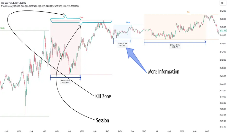
KillZones & Sessions [TradingFinder] Volume | Asia, London & NY🔵 Introduction
🟣 Session
The forex market operates 24 hours a day, 5 days a week, with only Saturdays and Sundays being off; traders often focus on one of the forex trading sessions instead of trying to trade in all markets 24 hours a day.
Trading sessions are time intervals during which a specific financial market is active and trades are conducted. The Asia, London, and New York sessions are the most important trading sessions throughout the 24-hour period, during which a significant amount of money and liquidity enters the market.
🟣 Kill Zone
Traders in financial markets profit from the difference between the price at which they buy or sell and the current market price. Traders have different time horizons for trading.
Among these, some traders engage in daily or even hourly trading and must operate during times when the market has desirable trading volumes and significant price movements.
Kill zones are segments of a session with higher trading volumes and price fluctuations compared to the rest of the session.
🔵 How to Use
🟣 Session Time
The "Asia Session" consists of two sessions: "Sydney" and "Tokyo." The beginning of this session, according to the "UTC" time zone, is at 23:00 and ends at 06:00. Similarly, the beginning of the "Asia KillZone," according to the "UTC" time zone, is at 23:00, and it ends at 03:55.
The "London Session" consists of two sessions: "Frankfurt" and "London." The beginning of this session, according to the "UTC" time zone, is at 07:00, and it ends at 14:25. Similarly, the beginning of the "London KillZone," according to the "UTC" time zone, is at 07:00, and it ends at 09:55.
The beginning of the "New York am" session, according to the "UTC" time zone, is at 14:30, and it ends at 19:25. Similarly, the beginning of the "New York am KillZone," according to the "UTC" time zone, is at 14:30, and it ends at 16:55.
The beginning of the "New York pm" session, according to the "UTC" time zone, is at 19:30, and it ends at 22:55. Similarly, the beginning of the "New York pm KillZone," according to the "UTC" time zone, is at 19:30, and it ends at 20:55.
Important : To prevent session overlap, the working hours of each session have slightly changed.
🔵 Features
🟣 Simultaneous Session and Kill Zone
With this indicator, you can simultaneously view the kill zone and session. High and low lines are used to indicate sessions, while filled areas with color represent kill zones. If you do not want to see kill zones, you can turn off the display settings.
🟣 Candle, Time, and Volume
Using the "More Info" feature, you can see the number of candles, elapsed time, and traded volume within the colored filled area.
🔵 Settings
•Show More Info: To display "More Info," you need to turn on this feature and turn it off whenever you don't need it.
• You can also customize these settings for each session separately :
o Display or hide session.
o Choose session color.
o Set session time range.
o Display or hide kill zone.
o Set kill zone time range.
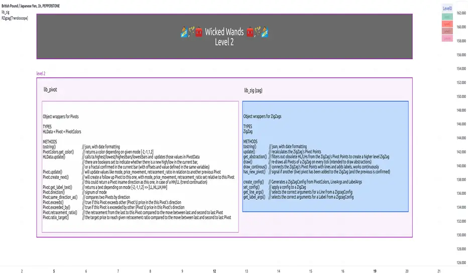
lib_zigLibrary "lib_zig"
Object oriented implementation of ZigZag
method tostring(this, date_format)
Namespace types: Zigzag
Parameters:
this (Zigzag)
date_format (simple string)
method update(this)
Namespace types: Zigzag
Parameters:
this (Zigzag)
method draw(this, colors)
Namespace types: Zigzag
Parameters:
this (Zigzag)
colors (PivotColors type from robbatt/lib_pivot/19)
Zigzag
Fields:
max_pivots (series__integer)
hldata (|robbatt/lib_pivot/19;HLData|#OBJ)
pivots (array__|robbatt/lib_pivot/19;Pivot|#OBJ)
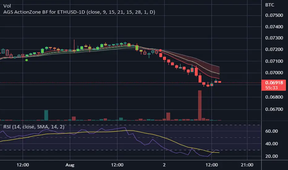
CDC ActionZone BF for ETHUSD-1D © PRoSkYNeT-EE
Based on improvements from "Kitti-Playbook Action Zone V.4.2.0.3 for Stock Market"
Based on improvements from "CDC Action Zone V3 2020 by piriya33"
Based on Triple MACD crossover between 9/15, 21/28, 15/28 for filter error signal (noise) from CDC ActionZone V3
MACDs generated from the execution of millions of times in the "Brute Force Algorithm" to backtest data from the past 5 years. ( 2017-08-21 to 2022-08-01 )
Released 2022-08-01
***** The indicator is used in the ETHUSD 1 Day period ONLY *****
Recommended Stop Loss : -4 % (execute stop Loss after candlestick has been closed)
Backtest Result ( Start $100 )
Winrate 63 % (Win:12, Loss:7, Total:19)
Live Days 1,806 days
B : Buy
S : Sell
SL : Stop Loss
2022-07-19 07 - 1,542 : B 6.971 ETH
2022-04-13 07 - 3,118 : S 8.98 % $10,750 12,7,19 63 %
2022-03-20 07 - 2,861 : B 3.448 ETH
2021-12-03 07 - 4,216 : SL -8.94 % $9,864 11,7,18 61 %
2021-11-30 07 - 4,630 : B 2.340 ETH
2021-11-18 07 - 3,997 : S 13.71 % $10,832 11,6,17 65 %
2021-10-05 07 - 3,515 : B 2.710 ETH
2021-09-20 07 - 2,977 : S 29.38 % $9,526 10,6,16 63 %
2021-07-28 07 - 2,301 : B 3.200 ETH
2021-05-20 07 - 2,769 : S 50.49 % $7,363 9,6,15 60 %
2021-03-30 07 - 1,840 : B 2.659 ETH
2021-03-22 07 - 1,681 : SL -8.29 % $4,893 8,6,14 57 %
2021-03-08 07 - 1,833 : B 2.911 ETH
2021-02-26 07 - 1,445 : S 279.27 % $5,335 8,5,13 62 %
2020-10-13 07 - 381 : B 3.692 ETH
2020-09-05 07 - 335 : S 38.43 % $1,407 7,5,12 58 %
2020-07-06 07 - 242 : B 4.199 ETH
2020-06-27 07 - 221 : S 28.49 % $1,016 6,5,11 55 %
2020-04-16 07 - 172 : B 4.598 ETH
2020-02-29 07 - 217 : S 47.62 % $791 5,5,10 50 %
2020-01-12 07 - 147 : B 3.644 ETH
2019-11-18 07 - 178 : S -2.73 % $536 4,5,9 44 %
2019-11-01 07 - 183 : B 3.010 ETH
2019-09-23 07 - 201 : SL -4.29 % $551 4,4,8 50 %
2019-09-18 07 - 210 : B 2.740 ETH
2019-07-12 07 - 275 : S 63.69 % $575 4,3,7 57 %
2019-05-03 07 - 168 : B 2.093 ETH
2019-04-28 07 - 158 : S 29.51 % $352 3,3,6 50 %
2019-02-15 07 - 122 : B 2.225 ETH
2019-01-10 07 - 125 : SL -6.02 % $271 2,3,5 40 %
2018-12-29 07 - 133 : B 2.172 ETH
2018-05-22 07 - 641 : S 5.95 % $289 2,2,4 50 %
2018-04-21 07 - 605 : B 0.451 ETH
2018-02-02 07 - 922 : S 197.42 % $273 1,2,3 33 %
2017-11-11 07 - 310 : B 0.296 ETH
2017-10-09 07 - 297 : SL -4.50 % $92 0,2,2 0 %
2017-10-07 07 - 311 : B 0.309 ETH
2017-08-22 07 - 310 : SL -4.02 % $96 0,1,1 0 %
2017-08-21 07 - 323 : B 0.310 ETH
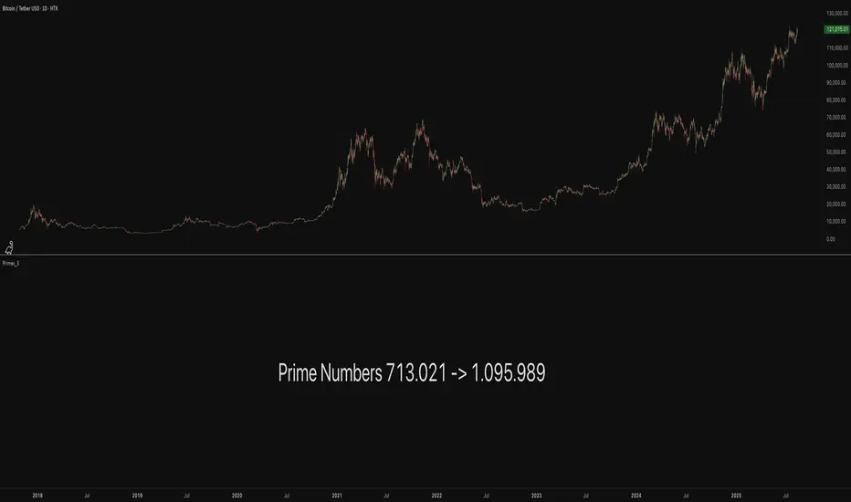
Primes_3These libraries (Primes_1 -> Primes_4) contain arrays of reduced Prime Numbers to minimize the amount of tokens, allowing more information to be exported.
Values, for example:
7001, 7013, 7019, 7027, 7039, 7043, 7057, 7069, 7079, 7103, 7109, 7021
are reduced to:
7001, 13, 19, 27, 39, 43, 57, 69, 79, 7103, 9, 21
With the restoreValues() function found in the Primes_4 library, the reduced values can be restored back to its original state.
7001, 13, 19, 27, 39, 43, 57, 69, 79, 7103, 9, 21
is restored back to:
7001, 7013, 7019, 7027, 7039, 7043, 7057, 7069, 7079, 7103, 7109, 7021
The libraries contain all Prime Numbers from 2 to 1.340.011
------------------------------------------------------------
Library "Primes_3"
Prime Numbers 713.021 - 1.095.989
primes_a()
Prime numbers 713.021 - 820.997
primes_b()
Prime numbers 821.003 - 928.979
primes_c()
Prime numbers 929.003 - 1.038.953
primes_d()
Prime numbers 1.039.001 - 1.095.989
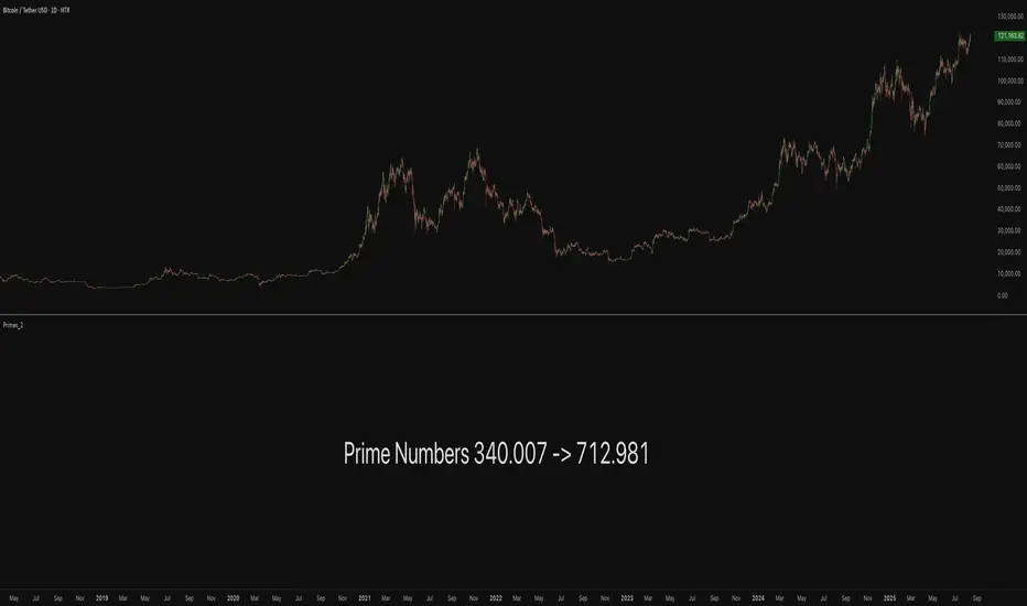
Primes_2These libraries (Primes_1 -> Primes_4) contain arrays of reduced Prime Numbers to minimize the amount of tokens, allowing more information to be exported.
Values, for example:
7001, 7013, 7019, 7027, 7039, 7043, 7057, 7069, 7079, 7103, 7109, 7021
are reduced to:
7001, 13, 19, 27, 39, 43, 57, 69, 79, 7103, 9, 21
With the restoreValues() function found in the Primes_4 library, the reduced values can be restored back to its original state.
7001, 13, 19, 27, 39, 43, 57, 69, 79, 7103, 9, 21
is restored back to:
7001, 7013, 7019, 7027, 7039, 7043, 7057, 7069, 7079, 7103, 7109, 7021
The libraries contain all Prime Numbers from 2 to 1.340.011
------------------------------------------------------------
Library "Primes_2"
Prime Numbers 340.007 - 712.981
primes_a()
Prime numbers 340.007 - 441.971
primes_b()
Prime numbers 442.003 - 545.959
primes_c()
Prime numbers 546.001 - 650.987
primes_d()
Prime numbers 651.017 - 712.981
Primes_1These libraries (Primes_1 -> Primes_4) contain arrays of reduced Prime Numbers to minimize the amount of tokens, allowing more information to be exported.
Values, for example:
7001, 7013, 7019, 7027, 7039, 7043, 7057, 7069, 7079, 7103, 7109, 7021
are reduced to:
7001, 13, 19, 27, 39, 43, 57, 69, 79, 7103, 9, 21
With the restoreValues() function found in the Primes_4 library, the reduced values can be restored back to its original state.
7001, 13, 19, 27, 39, 43, 57, 69, 79, 7103, 9, 21
is restored back to:
7001, 7013, 7019, 7027, 7039, 7043, 7057, 7069, 7079, 7103, 7109, 7021
The libraries contain all Prime Numbers from 2 to 1.340.011
------------------------------------------------------------
Library "Primes_1"
Prime Numbers 2 - 339.991
primes_a()
Prime numbers 2 - 81.689
primes_b()
Prime numbers 81.701 - 175.897
primes_c()
Prime numbers 175.909 - 273.997
primes_d()
Prime numbers 274.007 - 339.991

Kelly Position Size CalculatorThis position sizing calculator implements the Kelly Criterion, developed by John L. Kelly Jr. at Bell Laboratories in 1956, to determine mathematically optimal position sizes for maximizing long-term wealth growth. Unlike arbitrary position sizing methods, this tool provides a scientifically solution based on your strategy's actual performance statistics and incorporates modern refinements from over six decades of academic research.
The Kelly Criterion addresses a fundamental question in capital allocation: "What fraction of capital should be allocated to each opportunity to maximize growth while avoiding ruin?" This question has profound implications for financial markets, where traders and investors constantly face decisions about optimal capital allocation (Van Tharp, 2007).
Theoretical Foundation
The Kelly Criterion for binary outcomes is expressed as f* = (bp - q) / b, where f* represents the optimal fraction of capital to allocate, b denotes the risk-reward ratio, p indicates the probability of success, and q represents the probability of loss (Kelly, 1956). This formula maximizes the expected logarithm of wealth, ensuring maximum long-term growth rate while avoiding the risk of ruin.
The mathematical elegance of Kelly's approach lies in its derivation from information theory. Kelly's original work was motivated by Claude Shannon's information theory (Shannon, 1948), recognizing that maximizing the logarithm of wealth is equivalent to maximizing the rate of information transmission. This connection between information theory and wealth accumulation provides a deep theoretical foundation for optimal position sizing.
The logarithmic utility function underlying the Kelly Criterion naturally embodies several desirable properties for capital management. It exhibits decreasing marginal utility, penalizes large losses more severely than it rewards equivalent gains, and focuses on geometric rather than arithmetic mean returns, which is appropriate for compounding scenarios (Thorp, 2006).
Scientific Implementation
This calculator extends beyond basic Kelly implementation by incorporating state of the art refinements from academic research:
Parameter Uncertainty Adjustment: Following Michaud (1989), the implementation applies Bayesian shrinkage to account for parameter estimation error inherent in small sample sizes. The adjustment formula f_adjusted = f_kelly × confidence_factor + f_conservative × (1 - confidence_factor) addresses the overconfidence bias documented by Baker and McHale (2012), where the confidence factor increases with sample size and the conservative estimate equals 0.25 (quarter Kelly).
Sample Size Confidence: The reliability of Kelly calculations depends critically on sample size. Research by Browne and Whitt (1996) provides theoretical guidance on minimum sample requirements, suggesting that at least 30 independent observations are necessary for meaningful parameter estimates, with 100 or more trades providing reliable estimates for most trading strategies.
Universal Asset Compatibility: The calculator employs intelligent asset detection using TradingView's built-in symbol information, automatically adapting calculations for different asset classes without manual configuration.
ASSET SPECIFIC IMPLEMENTATION
Equity Markets: For stocks and ETFs, position sizing follows the calculation Shares = floor(Kelly Fraction × Account Size / Share Price). This straightforward approach reflects whole share constraints while accommodating fractional share trading capabilities.
Foreign Exchange Markets: Forex markets require lot-based calculations following Lot Size = Kelly Fraction × Account Size / (100,000 × Base Currency Value). The calculator automatically handles major currency pairs with appropriate pip value calculations, following industry standards described by Archer (2010).
Futures Markets: Futures position sizing accounts for leverage and margin requirements through Contracts = floor(Kelly Fraction × Account Size / Margin Requirement). The calculator estimates margin requirements as a percentage of contract notional value, with specific adjustments for micro-futures contracts that have smaller sizes and reduced margin requirements (Kaufman, 2013).
Index and Commodity Markets: These markets combine characteristics of both equity and futures markets. The calculator automatically detects whether instruments are cash-settled or futures-based, applying appropriate sizing methodologies with correct point value calculations.
Risk Management Integration
The calculator integrates sophisticated risk assessment through two primary modes:
Stop Loss Integration: When fixed stop-loss levels are defined, risk calculation follows Risk per Trade = Position Size × Stop Loss Distance. This ensures that the Kelly fraction accounts for actual risk exposure rather than theoretical maximum loss, with stop-loss distance measured in appropriate units for each asset class.
Strategy Drawdown Assessment: For discretionary exit strategies, risk estimation uses maximum historical drawdown through Risk per Trade = Position Value × (Maximum Drawdown / 100). This approach assumes that individual trade losses will not exceed the strategy's historical maximum drawdown, providing a reasonable estimate for strategies with well-defined risk characteristics.
Fractional Kelly Approaches
Pure Kelly sizing can produce substantial volatility, leading many practitioners to adopt fractional Kelly approaches. MacLean, Sanegre, Zhao, and Ziemba (2004) analyze the trade-offs between growth rate and volatility, demonstrating that half-Kelly typically reduces volatility by approximately 75% while sacrificing only 25% of the growth rate.
The calculator provides three primary Kelly modes to accommodate different risk preferences and experience levels. Full Kelly maximizes growth rate while accepting higher volatility, making it suitable for experienced practitioners with strong risk tolerance and robust capital bases. Half Kelly offers a balanced approach popular among professional traders, providing optimal risk-return balance by reducing volatility significantly while maintaining substantial growth potential. Quarter Kelly implements a conservative approach with low volatility, recommended for risk-averse traders or those new to Kelly methodology who prefer gradual introduction to optimal position sizing principles.
Empirical Validation and Performance
Extensive academic research supports the theoretical advantages of Kelly sizing. Hakansson and Ziemba (1995) provide a comprehensive review of Kelly applications in finance, documenting superior long-term performance across various market conditions and asset classes. Estrada (2008) analyzes Kelly performance in international equity markets, finding that Kelly-based strategies consistently outperform fixed position sizing approaches over extended periods across 19 developed markets over a 30-year period.
Several prominent investment firms have successfully implemented Kelly-based position sizing. Pabrai (2007) documents the application of Kelly principles at Berkshire Hathaway, noting Warren Buffett's concentrated portfolio approach aligns closely with Kelly optimal sizing for high-conviction investments. Quantitative hedge funds, including Renaissance Technologies and AQR, have incorporated Kelly-based risk management into their systematic trading strategies.
Practical Implementation Guidelines
Successful Kelly implementation requires systematic application with attention to several critical factors:
Parameter Estimation: Accurate parameter estimation represents the greatest challenge in practical Kelly implementation. Brown (1976) notes that small errors in probability estimates can lead to significant deviations from optimal performance. The calculator addresses this through Bayesian adjustments and confidence measures.
Sample Size Requirements: Users should begin with conservative fractional Kelly approaches until achieving sufficient historical data. Strategies with fewer than 30 trades may produce unreliable Kelly estimates, regardless of adjustments. Full confidence typically requires 100 or more independent trade observations.
Market Regime Considerations: Parameters that accurately describe historical performance may not reflect future market conditions. Ziemba (2003) recommends regular parameter updates and conservative adjustments when market conditions change significantly.
Professional Features and Customization
The calculator provides comprehensive customization options for professional applications:
Multiple Color Schemes: Eight professional color themes (Gold, EdgeTools, Behavioral, Quant, Ocean, Fire, Matrix, Arctic) with dark and light theme compatibility ensure optimal visibility across different trading environments.
Flexible Display Options: Adjustable table size and position accommodate various chart layouts and user preferences, while maintaining analytical depth and clarity.
Comprehensive Results: The results table presents essential information including asset specifications, strategy statistics, Kelly calculations, sample confidence measures, position values, risk assessments, and final position sizes in appropriate units for each asset class.
Limitations and Considerations
Like any analytical tool, the Kelly Criterion has important limitations that users must understand:
Stationarity Assumption: The Kelly Criterion assumes that historical strategy statistics represent future performance characteristics. Non-stationary market conditions may invalidate this assumption, as noted by Lo and MacKinlay (1999).
Independence Requirement: Each trade should be independent to avoid correlation effects. Many trading strategies exhibit serial correlation in returns, which can affect optimal position sizing and may require adjustments for portfolio applications.
Parameter Sensitivity: Kelly calculations are sensitive to parameter accuracy. Regular calibration and conservative approaches are essential when parameter uncertainty is high.
Transaction Costs: The implementation incorporates user-defined transaction costs but assumes these remain constant across different position sizes and market conditions, following Ziemba (2003).
Advanced Applications and Extensions
Multi-Asset Portfolio Considerations: While this calculator optimizes individual position sizes, portfolio-level applications require additional considerations for correlation effects and aggregate risk management. Simplified portfolio approaches include treating positions independently with correlation adjustments.
Behavioral Factors: Behavioral finance research reveals systematic biases that can interfere with Kelly implementation. Kahneman and Tversky (1979) document loss aversion, overconfidence, and other cognitive biases that lead traders to deviate from optimal strategies. Successful implementation requires disciplined adherence to calculated recommendations.
Time-Varying Parameters: Advanced implementations may incorporate time-varying parameter models that adjust Kelly recommendations based on changing market conditions, though these require sophisticated econometric techniques and substantial computational resources.
Comprehensive Usage Instructions and Practical Examples
Implementation begins with loading the calculator on your desired trading instrument's chart. The system automatically detects asset type across stocks, forex, futures, and cryptocurrency markets while extracting current price information. Navigation to the indicator settings allows input of your specific strategy parameters.
Strategy statistics configuration requires careful attention to several key metrics. The win rate should be calculated from your backtest results using the formula of winning trades divided by total trades multiplied by 100. Average win represents the sum of all profitable trades divided by the number of winning trades, while average loss calculates the sum of all losing trades divided by the number of losing trades, entered as a positive number. The total historical trades parameter requires the complete number of trades in your backtest, with a minimum of 30 trades recommended for basic functionality and 100 or more trades optimal for statistical reliability. Account size should reflect your available trading capital, specifically the risk capital allocated for trading rather than total net worth.
Risk management configuration adapts to your specific trading approach. The stop loss setting should be enabled if you employ fixed stop-loss exits, with the stop loss distance specified in appropriate units depending on the asset class. For stocks, this distance is measured in dollars, for forex in pips, and for futures in ticks. When stop losses are not used, the maximum strategy drawdown percentage from your backtest provides the risk assessment baseline. Kelly mode selection offers three primary approaches: Full Kelly for aggressive growth with higher volatility suitable for experienced practitioners, Half Kelly for balanced risk-return optimization popular among professional traders, and Quarter Kelly for conservative approaches with reduced volatility.
Display customization ensures optimal integration with your trading environment. Eight professional color themes provide optimization for different chart backgrounds and personal preferences. Table position selection allows optimal placement within your chart layout, while table size adjustment ensures readability across different screen resolutions and viewing preferences.
Detailed Practical Examples
Example 1: SPY Swing Trading Strategy
Consider a professionally developed swing trading strategy for SPY (S&P 500 ETF) with backtesting results spanning 166 total trades. The strategy achieved 110 winning trades, representing a 66.3% win rate, with an average winning trade of $2,200 and average losing trade of $862. The maximum drawdown reached 31.4% during the testing period, and the available trading capital amounts to $25,000. This strategy employs discretionary exits without fixed stop losses.
Implementation requires loading the calculator on the SPY daily chart and configuring the parameters accordingly. The win rate input receives 66.3, while average win and loss inputs receive 2200 and 862 respectively. Total historical trades input requires 166, with account size set to 25000. The stop loss function remains disabled due to the discretionary exit approach, with maximum strategy drawdown set to 31.4%. Half Kelly mode provides the optimal balance between growth and risk management for this application.
The calculator generates several key outputs for this scenario. The risk-reward ratio calculates automatically to 2.55, while the Kelly fraction reaches approximately 53% before scientific adjustments. Sample confidence achieves 100% given the 166 trades providing high statistical confidence. The recommended position settles at approximately 27% after Half Kelly and Bayesian adjustment factors. Position value reaches approximately $6,750, translating to 16 shares at a $420 SPY price. Risk per trade amounts to approximately $2,110, representing 31.4% of position value, with expected value per trade reaching approximately $1,466. This recommendation represents the mathematically optimal balance between growth potential and risk management for this specific strategy profile.
Example 2: EURUSD Day Trading with Stop Losses
A high-frequency EURUSD day trading strategy demonstrates different parameter requirements compared to swing trading approaches. This strategy encompasses 89 total trades with a 58% win rate, generating an average winning trade of $180 and average losing trade of $95. The maximum drawdown reached 12% during testing, with available capital of $10,000. The strategy employs fixed stop losses at 25 pips and take profit targets at 45 pips, providing clear risk-reward parameters.
Implementation begins with loading the calculator on the EURUSD 1-hour chart for appropriate timeframe alignment. Parameter configuration includes win rate at 58, average win at 180, and average loss at 95. Total historical trades input receives 89, with account size set to 10000. The stop loss function is enabled with distance set to 25 pips, reflecting the fixed exit strategy. Quarter Kelly mode provides conservative positioning due to the smaller sample size compared to the previous example.
Results demonstrate the impact of smaller sample sizes on Kelly calculations. The risk-reward ratio calculates to 1.89, while the Kelly fraction reaches approximately 32% before adjustments. Sample confidence achieves 89%, providing moderate statistical confidence given the 89 trades. The recommended position settles at approximately 7% after Quarter Kelly application and Bayesian shrinkage adjustment for the smaller sample. Position value amounts to approximately $700, translating to 0.07 standard lots. Risk per trade reaches approximately $175, calculated as 25 pips multiplied by lot size and pip value, with expected value per trade at approximately $49. This conservative position sizing reflects the smaller sample size, with position sizes expected to increase as trade count surpasses 100 and statistical confidence improves.
Example 3: ES1! Futures Systematic Strategy
Systematic futures trading presents unique considerations for Kelly criterion application, as demonstrated by an E-mini S&P 500 futures strategy encompassing 234 total trades. This systematic approach achieved a 45% win rate with an average winning trade of $1,850 and average losing trade of $720. The maximum drawdown reached 18% during the testing period, with available capital of $50,000. The strategy employs 15-tick stop losses with contract specifications of $50 per tick, providing precise risk control mechanisms.
Implementation involves loading the calculator on the ES1! 15-minute chart to align with the systematic trading timeframe. Parameter configuration includes win rate at 45, average win at 1850, and average loss at 720. Total historical trades receives 234, providing robust statistical foundation, with account size set to 50000. The stop loss function is enabled with distance set to 15 ticks, reflecting the systematic exit methodology. Half Kelly mode balances growth potential with appropriate risk management for futures trading.
Results illustrate how favorable risk-reward ratios can support meaningful position sizing despite lower win rates. The risk-reward ratio calculates to 2.57, while the Kelly fraction reaches approximately 16%, lower than previous examples due to the sub-50% win rate. Sample confidence achieves 100% given the 234 trades providing high statistical confidence. The recommended position settles at approximately 8% after Half Kelly adjustment. Estimated margin per contract amounts to approximately $2,500, resulting in a single contract allocation. Position value reaches approximately $2,500, with risk per trade at $750, calculated as 15 ticks multiplied by $50 per tick. Expected value per trade amounts to approximately $508. Despite the lower win rate, the favorable risk-reward ratio supports meaningful position sizing, with single contract allocation reflecting appropriate leverage management for futures trading.
Example 4: MES1! Micro-Futures for Smaller Accounts
Micro-futures contracts provide enhanced accessibility for smaller trading accounts while maintaining identical strategy characteristics. Using the same systematic strategy statistics from the previous example but with available capital of $15,000 and micro-futures specifications of $5 per tick with reduced margin requirements, the implementation demonstrates improved position sizing granularity.
Kelly calculations remain identical to the full-sized contract example, maintaining the same risk-reward dynamics and statistical foundations. However, estimated margin per contract reduces to approximately $250 for micro-contracts, enabling allocation of 4-5 micro-contracts. Position value reaches approximately $1,200, while risk per trade calculates to $75, derived from 15 ticks multiplied by $5 per tick. This granularity advantage provides better position size precision for smaller accounts, enabling more accurate Kelly implementation without requiring large capital commitments.
Example 5: Bitcoin Swing Trading
Cryptocurrency markets present unique challenges requiring modified Kelly application approaches. A Bitcoin swing trading strategy on BTCUSD encompasses 67 total trades with a 71% win rate, generating average winning trades of $3,200 and average losing trades of $1,400. Maximum drawdown reached 28% during testing, with available capital of $30,000. The strategy employs technical analysis for exits without fixed stop losses, relying on price action and momentum indicators.
Implementation requires conservative approaches due to cryptocurrency volatility characteristics. Quarter Kelly mode is recommended despite the high win rate to account for crypto market unpredictability. Expected position sizing remains reduced due to the limited sample size of 67 trades, requiring additional caution until statistical confidence improves. Regular parameter updates are strongly recommended due to cryptocurrency market evolution and changing volatility patterns that can significantly impact strategy performance characteristics.
Advanced Usage Scenarios
Portfolio position sizing requires sophisticated consideration when running multiple strategies simultaneously. Each strategy should have its Kelly fraction calculated independently to maintain mathematical integrity. However, correlation adjustments become necessary when strategies exhibit related performance patterns. Moderately correlated strategies should receive individual position size reductions of 10-20% to account for overlapping risk exposure. Aggregate portfolio risk monitoring ensures total exposure remains within acceptable limits across all active strategies. Professional practitioners often consider using lower fractional Kelly approaches, such as Quarter Kelly, when running multiple strategies simultaneously to provide additional safety margins.
Parameter sensitivity analysis forms a critical component of professional Kelly implementation. Regular validation procedures should include monthly parameter updates using rolling 100-trade windows to capture evolving market conditions while maintaining statistical relevance. Sensitivity testing involves varying win rates by ±5% and average win/loss ratios by ±10% to assess recommendation stability under different parameter assumptions. Out-of-sample validation reserves 20% of historical data for parameter verification, ensuring that optimization doesn't create curve-fitted results. Regime change detection monitors actual performance against expected metrics, triggering parameter reassessment when significant deviations occur.
Risk management integration requires professional overlay considerations beyond pure Kelly calculations. Daily loss limits should cease trading when daily losses exceed twice the calculated risk per trade, preventing emotional decision-making during adverse periods. Maximum position limits should never exceed 25% of account value in any single position regardless of Kelly recommendations, maintaining diversification principles. Correlation monitoring reduces position sizes when holding multiple correlated positions that move together during market stress. Volatility adjustments consider reducing position sizes during periods of elevated VIX above 25 for equity strategies, adapting to changing market conditions.
Troubleshooting and Optimization
Professional implementation often encounters specific challenges requiring systematic troubleshooting approaches. Zero position size displays typically result from insufficient capital for minimum position sizes, negative expected values, or extremely conservative Kelly calculations. Solutions include increasing account size, verifying strategy statistics for accuracy, considering Quarter Kelly mode for conservative approaches, or reassessing overall strategy viability when fundamental issues exist.
Extremely high Kelly fractions exceeding 50% usually indicate underlying problems with parameter estimation. Common causes include unrealistic win rates, inflated risk-reward ratios, or curve-fitted backtest results that don't reflect genuine trading conditions. Solutions require verifying backtest methodology, including all transaction costs in calculations, testing strategies on out-of-sample data, and using conservative fractional Kelly approaches until parameter reliability improves.
Low sample confidence below 50% reflects insufficient historical trades for reliable parameter estimation. This situation demands gathering additional trading data, using Quarter Kelly approaches until reaching 100 or more trades, applying extra conservatism in position sizing, and considering paper trading to build statistical foundations without capital risk.
Inconsistent results across similar strategies often stem from parameter estimation differences, market regime changes, or strategy degradation over time. Professional solutions include standardizing backtest methodology across all strategies, updating parameters regularly to reflect current conditions, and monitoring live performance against expectations to identify deteriorating strategies.
Position sizes that appear inappropriately large or small require careful validation against traditional risk management principles. Professional standards recommend never risking more than 2-3% per trade regardless of Kelly calculations. Calibration should begin with Quarter Kelly approaches, gradually increasing as comfort and confidence develop. Most institutional traders utilize 25-50% of full Kelly recommendations to balance growth with prudent risk management.
Market condition adjustments require dynamic approaches to Kelly implementation. Trending markets may support full Kelly recommendations when directional momentum provides favorable conditions. Ranging or volatile markets typically warrant reducing to Half or Quarter Kelly to account for increased uncertainty. High correlation periods demand reducing individual position sizes when multiple positions move together, concentrating risk exposure. News and event periods often justify temporary position size reductions during high-impact releases that can create unpredictable market movements.
Performance monitoring requires systematic protocols to ensure Kelly implementation remains effective over time. Weekly reviews should compare actual versus expected win rates and average win/loss ratios to identify parameter drift or strategy degradation. Position size efficiency and execution quality monitoring ensures that calculated recommendations translate effectively into actual trading results. Tracking correlation between calculated and realized risk helps identify discrepancies between theoretical and practical risk exposure.
Monthly calibration provides more comprehensive parameter assessment using the most recent 100 trades to maintain statistical relevance while capturing current market conditions. Kelly mode appropriateness requires reassessment based on recent market volatility and performance characteristics, potentially shifting between Full, Half, and Quarter Kelly approaches as conditions change. Transaction cost evaluation ensures that commission structures, spreads, and slippage estimates remain accurate and current.
Quarterly strategic reviews encompass comprehensive strategy performance analysis comparing long-term results against expectations and identifying trends in effectiveness. Market regime assessment evaluates parameter stability across different market conditions, determining whether strategy characteristics remain consistent or require fundamental adjustments. Strategic modifications to position sizing methodology may become necessary as markets evolve or trading approaches mature, ensuring that Kelly implementation continues supporting optimal capital allocation objectives.
Professional Applications
This calculator serves diverse professional applications across the financial industry. Quantitative hedge funds utilize the implementation for systematic position sizing within algorithmic trading frameworks, where mathematical precision and consistent application prove essential for institutional capital management. Professional discretionary traders benefit from optimized position management that removes emotional bias while maintaining flexibility for market-specific adjustments. Portfolio managers employ the calculator for developing risk-adjusted allocation strategies that enhance returns while maintaining prudent risk controls across diverse asset classes and investment strategies.
Individual traders seeking mathematical optimization of capital allocation find the calculator provides institutional-grade methodology previously available only to professional money managers. The Kelly Criterion establishes theoretical foundation for optimal capital allocation across both single strategies and multiple trading systems, offering significant advantages over arbitrary position sizing methods that rely on intuition or fixed percentage approaches. Professional implementation ensures consistent application of mathematically sound principles while adapting to changing market conditions and strategy performance characteristics.
Conclusion
The Kelly Criterion represents one of the few mathematically optimal solutions to fundamental investment problems. When properly understood and carefully implemented, it provides significant competitive advantage in financial markets. This calculator implements modern refinements to Kelly's original formula while maintaining accessibility for practical trading applications.
Success with Kelly requires ongoing learning, systematic application, and continuous refinement based on market feedback and evolving research. Users who master Kelly principles and implement them systematically can expect superior risk-adjusted returns and more consistent capital growth over extended periods.
The extensive academic literature provides rich resources for deeper study, while practical experience builds the intuition necessary for effective implementation. Regular parameter updates, conservative approaches with limited data, and disciplined adherence to calculated recommendations are essential for optimal results.
References
Archer, M. D. (2010). Getting Started in Currency Trading: Winning in Today's Forex Market (3rd ed.). John Wiley & Sons.
Baker, R. D., & McHale, I. G. (2012). An empirical Bayes approach to optimising betting strategies. Journal of the Royal Statistical Society: Series D (The Statistician), 61(1), 75-92.
Breiman, L. (1961). Optimal gambling systems for favorable games. In J. Neyman (Ed.), Proceedings of the Fourth Berkeley Symposium on Mathematical Statistics and Probability (pp. 65-78). University of California Press.
Brown, D. B. (1976). Optimal portfolio growth: Logarithmic utility and the Kelly criterion. In W. T. Ziemba & R. G. Vickson (Eds.), Stochastic Optimization Models in Finance (pp. 1-23). Academic Press.
Browne, S., & Whitt, W. (1996). Portfolio choice and the Bayesian Kelly criterion. Advances in Applied Probability, 28(4), 1145-1176.
Estrada, J. (2008). Geometric mean maximization: An overlooked portfolio approach? The Journal of Investing, 17(4), 134-147.
Hakansson, N. H., & Ziemba, W. T. (1995). Capital growth theory. In R. A. Jarrow, V. Maksimovic, & W. T. Ziemba (Eds.), Handbooks in Operations Research and Management Science (Vol. 9, pp. 65-86). Elsevier.
Kahneman, D., & Tversky, A. (1979). Prospect theory: An analysis of decision under risk. Econometrica, 47(2), 263-291.
Kaufman, P. J. (2013). Trading Systems and Methods (5th ed.). John Wiley & Sons.
Kelly Jr, J. L. (1956). A new interpretation of information rate. Bell System Technical Journal, 35(4), 917-926.
Lo, A. W., & MacKinlay, A. C. (1999). A Non-Random Walk Down Wall Street. Princeton University Press.
MacLean, L. C., Sanegre, E. O., Zhao, Y., & Ziemba, W. T. (2004). Capital growth with security. Journal of Economic Dynamics and Control, 28(4), 937-954.
MacLean, L. C., Thorp, E. O., & Ziemba, W. T. (2011). The Kelly Capital Growth Investment Criterion: Theory and Practice. World Scientific.
Michaud, R. O. (1989). The Markowitz optimization enigma: Is 'optimized' optimal? Financial Analysts Journal, 45(1), 31-42.
Pabrai, M. (2007). The Dhandho Investor: The Low-Risk Value Method to High Returns. John Wiley & Sons.
Shannon, C. E. (1948). A mathematical theory of communication. Bell System Technical Journal, 27(3), 379-423.
Tharp, V. K. (2007). Trade Your Way to Financial Freedom (2nd ed.). McGraw-Hill.
Thorp, E. O. (2006). The Kelly criterion in blackjack sports betting, and the stock market. In L. C. MacLean, E. O. Thorp, & W. T. Ziemba (Eds.), The Kelly Capital Growth Investment Criterion: Theory and Practice (pp. 789-832). World Scientific.
Van Tharp, K. (2007). Trade Your Way to Financial Freedom (2nd ed.). McGraw-Hill Education.
Vince, R. (1992). The Mathematics of Money Management: Risk Analysis Techniques for Traders. John Wiley & Sons.
Vince, R., & Zhu, H. (2015). Optimal betting under parameter uncertainty. Journal of Statistical Planning and Inference, 161, 19-31.
Ziemba, W. T. (2003). The Stochastic Programming Approach to Asset, Liability, and Wealth Management. The Research Foundation of AIMR.
Further Reading
For comprehensive understanding of Kelly Criterion applications and advanced implementations:
MacLean, L. C., Thorp, E. O., & Ziemba, W. T. (2011). The Kelly Capital Growth Investment Criterion: Theory and Practice. World Scientific.
Vince, R. (1992). The Mathematics of Money Management: Risk Analysis Techniques for Traders. John Wiley & Sons.
Thorp, E. O. (2017). A Man for All Markets: From Las Vegas to Wall Street. Random House.
Cover, T. M., & Thomas, J. A. (2006). Elements of Information Theory (2nd ed.). John Wiley & Sons.
Ziemba, W. T., & Vickson, R. G. (Eds.). (2006). Stochastic Optimization Models in Finance. World Scientific.

Gold Killzone Bias Suite🟡 Gold Killzone Bias Suite
The Gold Killzone Bias Suite is an advanced institutional-grade tool designed to generate high-confidence directional bias for XAU/USD (Gold) during the London and New York killzones.
Built for traders using a structured, confluence-driven approach, this tool blends price action, smart money principles, momentum, and volume into a real-time bias engine with a clean, easy-to-read dashboard.
🔧 Key Features
🕰️ Session-Based Bias (London / New York)
Independent bias calculation per session
Killzone times customizable with timezone support
Background highlighting (blue/red) for each session
📊 VWAP Engine
Reclaim & rejection detection
VWAP deviation alerts
Daily HTF VWAP integration
Score impact based on VWAP behaviour
📉 Market Structure (CHoCH / BOS)
Detects swing highs/lows
Labels bullish/bearish CHoCHs
Structure score contributes to session bias
💧 Liquidity Grabs
Detects stop hunts above highs / below lows
Confirms with candle rejection (body % filter)
Plots labels and adds to bias scoring
⚡ Momentum Filters
RSI: Bullish >55, Bearish <45
MACD: Histogram + Signal Line crossovers
Combined momentum score used in bias
🧠 Smart Money Proximity
Optional FVG/OB score toggle (placeholder for custom logic)
Adds static confluence for proximity-based setups
⏫ Higher Time Frame Context
Daily VWAP comparison
4H high/low structure breaks
Adds trend score to current session bias
🧠 How Bias Works
The suite uses a scoring model. Each confluence adds or subtracts points:
VWAP reclaim/reject: ±30
CHoCH/BOS: ±30
Liquidity grab: ±20
RSI/MACD: ±10
FVG/OB Proximity: +10
Daily VWAP trend: ±10
H4 Trend Break: ±10
Final Bias:
Bullish if score ≥ +20
Bearish if score ≤ -20
Neutral if between -19 and +19
A confidence % (capped at 100) is also shown, along with the contributing confluences (VWAP, Structure, Liquidity, etc.).
📋 Dashboard
A real-time dashboard shows for each session:
Session name and time
Bias (Bullish / Bearish / Neutral)
Confidence (%)
Confluences used
Position can be moved (Top Left, Top Right, etc.). Designed to be unobtrusive yet informative.
🧪 Best Practices
Use on 15m / 5m charts for intraday setups
Confirm with D1 or H4 structure for directional context
Combine with OB/FVG zones or SMT for entries
Use Trading View alerts for bias flips or liquidity grabs (custom logic can be added)
Bar Replay compatible for back testing and journaling bias shifts
🔐 Notes
Does not generate trade signals or alerts by default
Focused on bias generation and confluence stacking
Compatible with funded account trading models
📈 Built for traders who want a systematic, score-based approach to identifying directional edge in high-volume gold sessions.

Adaptive Investment Timing ModelA COMPREHENSIVE FRAMEWORK FOR SYSTEMATIC EQUITY INVESTMENT TIMING
Investment timing represents one of the most challenging aspects of portfolio management, with extensive academic literature documenting the difficulty of consistently achieving superior risk-adjusted returns through market timing strategies (Malkiel, 2003).
Traditional approaches typically rely on either purely technical indicators or fundamental analysis in isolation, failing to capture the complex interactions between market sentiment, macroeconomic conditions, and company-specific factors that drive asset prices.
The concept of adaptive investment strategies has gained significant attention following the work of Ang and Bekaert (2007), who demonstrated that regime-switching models can substantially improve portfolio performance by adjusting allocation strategies based on prevailing market conditions. Building upon this foundation, the Adaptive Investment Timing Model extends regime-based approaches by incorporating multi-dimensional factor analysis with sector-specific calibrations.
Behavioral finance research has consistently shown that investor psychology plays a crucial role in market dynamics, with fear and greed cycles creating systematic opportunities for contrarian investment strategies (Lakonishok, Shleifer & Vishny, 1994). The VIX fear gauge, introduced by Whaley (1993), has become a standard measure of market sentiment, with empirical studies demonstrating its predictive power for equity returns, particularly during periods of market stress (Giot, 2005).
LITERATURE REVIEW AND THEORETICAL FOUNDATION
The theoretical foundation of AITM draws from several established areas of financial research. Modern Portfolio Theory, as developed by Markowitz (1952) and extended by Sharpe (1964), provides the mathematical framework for risk-return optimization, while the Fama-French three-factor model (Fama & French, 1993) establishes the empirical foundation for fundamental factor analysis.
Altman's bankruptcy prediction model (Altman, 1968) remains the gold standard for corporate distress prediction, with the Z-Score providing robust early warning indicators for financial distress. Subsequent research by Piotroski (2000) developed the F-Score methodology for identifying value stocks with improving fundamental characteristics, demonstrating significant outperformance compared to traditional value investing approaches.
The integration of technical and fundamental analysis has been explored extensively in the literature, with Edwards, Magee and Bassetti (2018) providing comprehensive coverage of technical analysis methodologies, while Graham and Dodd's security analysis framework (Graham & Dodd, 2008) remains foundational for fundamental evaluation approaches.
Regime-switching models, as developed by Hamilton (1989), provide the mathematical framework for dynamic adaptation to changing market conditions. Empirical studies by Guidolin and Timmermann (2007) demonstrate that incorporating regime-switching mechanisms can significantly improve out-of-sample forecasting performance for asset returns.
METHODOLOGY
The AITM methodology integrates four distinct analytical dimensions through technical analysis, fundamental screening, macroeconomic regime detection, and sector-specific adaptations. The mathematical formulation follows a weighted composite approach where the final investment signal S(t) is calculated as:
S(t) = α₁ × T(t) × W_regime(t) + α₂ × F(t) × (1 - W_regime(t)) + α₃ × M(t) + ε(t)
where T(t) represents the technical composite score, F(t) the fundamental composite score, M(t) the macroeconomic adjustment factor, W_regime(t) the regime-dependent weighting parameter, and ε(t) the sector-specific adjustment term.
Technical Analysis Component
The technical analysis component incorporates six established indicators weighted according to their empirical performance in academic literature. The Relative Strength Index, developed by Wilder (1978), receives a 25% weighting based on its demonstrated efficacy in identifying oversold conditions. Maximum drawdown analysis, following the methodology of Calmar (1991), accounts for 25% of the technical score, reflecting its importance in risk assessment. Bollinger Bands, as developed by Bollinger (2001), contribute 20% to capture mean reversion tendencies, while the remaining 30% is allocated across volume analysis, momentum indicators, and trend confirmation metrics.
Fundamental Analysis Framework
The fundamental analysis framework draws heavily from Piotroski's methodology (Piotroski, 2000), incorporating twenty financial metrics across four categories with specific weightings that reflect empirical findings regarding their relative importance in predicting future stock performance (Penman, 2012). Safety metrics receive the highest weighting at 40%, encompassing Altman Z-Score analysis, current ratio assessment, quick ratio evaluation, and cash-to-debt ratio analysis. Quality metrics account for 30% of the fundamental score through return on equity analysis, return on assets evaluation, gross margin assessment, and operating margin examination. Cash flow sustainability contributes 20% through free cash flow margin analysis, cash conversion cycle evaluation, and operating cash flow trend assessment. Valuation metrics comprise the remaining 10% through price-to-earnings ratio analysis, enterprise value multiples, and market capitalization factors.
Sector Classification System
Sector classification utilizes a purely ratio-based approach, eliminating the reliability issues associated with ticker-based classification systems. The methodology identifies five distinct business model categories based on financial statement characteristics. Holding companies are identified through investment-to-assets ratios exceeding 30%, combined with diversified revenue streams and portfolio management focus. Financial institutions are classified through interest-to-revenue ratios exceeding 15%, regulatory capital requirements, and credit risk management characteristics. Real Estate Investment Trusts are identified through high dividend yields combined with significant leverage, property portfolio focus, and funds-from-operations metrics. Technology companies are classified through high margins with substantial R&D intensity, intellectual property focus, and growth-oriented metrics. Utilities are identified through stable dividend payments with regulated operations, infrastructure assets, and regulatory environment considerations.
Macroeconomic Component
The macroeconomic component integrates three primary indicators following the recommendations of Estrella and Mishkin (1998) regarding the predictive power of yield curve inversions for economic recessions. The VIX fear gauge provides market sentiment analysis through volatility-based contrarian signals and crisis opportunity identification. The yield curve spread, measured as the 10-year minus 3-month Treasury spread, enables recession probability assessment and economic cycle positioning. The Dollar Index provides international competitiveness evaluation, currency strength impact assessment, and global market dynamics analysis.
Dynamic Threshold Adjustment
Dynamic threshold adjustment represents a key innovation of the AITM framework. Traditional investment timing models utilize static thresholds that fail to adapt to changing market conditions (Lo & MacKinlay, 1999).
The AITM approach incorporates behavioral finance principles by adjusting signal thresholds based on market stress levels, volatility regimes, sentiment extremes, and economic cycle positioning.
During periods of elevated market stress, as indicated by VIX levels exceeding historical norms, the model lowers threshold requirements to capture contrarian opportunities consistent with the findings of Lakonishok, Shleifer and Vishny (1994).
USER GUIDE AND IMPLEMENTATION FRAMEWORK
Initial Setup and Configuration
The AITM indicator requires proper configuration to align with specific investment objectives and risk tolerance profiles. Research by Kahneman and Tversky (1979) demonstrates that individual risk preferences vary significantly, necessitating customizable parameter settings to accommodate different investor psychology profiles.
Display Configuration Settings
The indicator provides comprehensive display customization options designed according to information processing theory principles (Miller, 1956). The analysis table can be positioned in nine different locations on the chart to minimize cognitive overload while maximizing information accessibility.
Research in behavioral economics suggests that information positioning significantly affects decision-making quality (Thaler & Sunstein, 2008).
Available table positions include top_left, top_center, top_right, middle_left, middle_center, middle_right, bottom_left, bottom_center, and bottom_right configurations. Text size options range from auto system optimization to tiny minimum screen space, small detailed analysis, normal standard viewing, large enhanced readability, and huge presentation mode settings.
Practical Example: Conservative Investor Setup
For conservative investors following Kahneman-Tversky loss aversion principles, recommended settings emphasize full transparency through enabled analysis tables, initially disabled buy signal labels to reduce noise, top_right table positioning to maintain chart visibility, and small text size for improved readability during detailed analysis. Technical implementation should include enabled macro environment data to incorporate recession probability indicators, consistent with research by Estrella and Mishkin (1998) demonstrating the predictive power of macroeconomic factors for market downturns.
Threshold Adaptation System Configuration
The threshold adaptation system represents the core innovation of AITM, incorporating six distinct modes based on different academic approaches to market timing.
Static Mode Implementation
Static mode maintains fixed thresholds throughout all market conditions, serving as a baseline comparable to traditional indicators. Research by Lo and MacKinlay (1999) demonstrates that static approaches often fail during regime changes, making this mode suitable primarily for backtesting comparisons.
Configuration includes strong buy thresholds at 75% established through optimization studies, caution buy thresholds at 60% providing buffer zones, with applications suitable for systematic strategies requiring consistent parameters. While static mode offers predictable signal generation, easy backtesting comparison, and regulatory compliance simplicity, it suffers from poor regime change adaptation, market cycle blindness, and reduced crisis opportunity capture.
Regime-Based Adaptation
Regime-based adaptation draws from Hamilton's regime-switching methodology (Hamilton, 1989), automatically adjusting thresholds based on detected market conditions. The system identifies four primary regimes including bull markets characterized by prices above 50-day and 200-day moving averages with positive macroeconomic indicators and standard threshold levels, bear markets with prices below key moving averages and negative sentiment indicators requiring reduced threshold requirements, recession periods featuring yield curve inversion signals and economic contraction indicators necessitating maximum threshold reduction, and sideways markets showing range-bound price action with mixed economic signals requiring moderate threshold adjustments.
Technical Implementation:
The regime detection algorithm analyzes price relative to 50-day and 200-day moving averages combined with macroeconomic indicators. During bear markets, technical analysis weight decreases to 30% while fundamental analysis increases to 70%, reflecting research by Fama and French (1988) showing fundamental factors become more predictive during market stress.
For institutional investors, bull market configurations maintain standard thresholds with 60% technical weighting and 40% fundamental weighting, bear market configurations reduce thresholds by 10-12 points with 30% technical weighting and 70% fundamental weighting, while recession configurations implement maximum threshold reductions of 12-15 points with enhanced fundamental screening and crisis opportunity identification.
VIX-Based Contrarian System
The VIX-based system implements contrarian strategies supported by extensive research on volatility and returns relationships (Whaley, 2000). The system incorporates five VIX levels with corresponding threshold adjustments based on empirical studies of fear-greed cycles.
Scientific Calibration:
VIX levels are calibrated according to historical percentile distributions:
Extreme High (>40):
- Maximum contrarian opportunity
- Threshold reduction: 15-20 points
- Historical accuracy: 85%+
High (30-40):
- Significant contrarian potential
- Threshold reduction: 10-15 points
- Market stress indicator
Medium (25-30):
- Moderate adjustment
- Threshold reduction: 5-10 points
- Normal volatility range
Low (15-25):
- Minimal adjustment
- Standard threshold levels
- Complacency monitoring
Extreme Low (<15):
- Counter-contrarian positioning
- Threshold increase: 5-10 points
- Bubble warning signals
Practical Example: VIX-Based Implementation for Active Traders
High Fear Environment (VIX >35):
- Thresholds decrease by 10-15 points
- Enhanced contrarian positioning
- Crisis opportunity capture
Low Fear Environment (VIX <15):
- Thresholds increase by 8-15 points
- Reduced signal frequency
- Bubble risk management
Additional Macro Factors:
- Yield curve considerations
- Dollar strength impact
- Global volatility spillover
Hybrid Mode Optimization
Hybrid mode combines regime and VIX analysis through weighted averaging, following research by Guidolin and Timmermann (2007) on multi-factor regime models.
Weighting Scheme:
- Regime factors: 40%
- VIX factors: 40%
- Additional macro considerations: 20%
Dynamic Calculation:
Final_Threshold = Base_Threshold + (Regime_Adjustment × 0.4) + (VIX_Adjustment × 0.4) + (Macro_Adjustment × 0.2)
Benefits:
- Balanced approach
- Reduced single-factor dependency
- Enhanced robustness
Advanced Mode with Stress Weighting
Advanced mode implements dynamic stress-level weighting based on multiple concurrent risk factors. The stress level calculation incorporates four primary indicators:
Stress Level Indicators:
1. Yield curve inversion (recession predictor)
2. Volatility spikes (market disruption)
3. Severe drawdowns (momentum breaks)
4. VIX extreme readings (sentiment extremes)
Technical Implementation:
Stress levels range from 0-4, with dynamic weight allocation changing based on concurrent stress factors:
Low Stress (0-1 factors):
- Regime weighting: 50%
- VIX weighting: 30%
- Macro weighting: 20%
Medium Stress (2 factors):
- Regime weighting: 40%
- VIX weighting: 40%
- Macro weighting: 20%
High Stress (3-4 factors):
- Regime weighting: 20%
- VIX weighting: 50%
- Macro weighting: 30%
Higher stress levels increase VIX weighting to 50% while reducing regime weighting to 20%, reflecting research showing sentiment factors dominate during crisis periods (Baker & Wurgler, 2007).
Percentile-Based Historical Analysis
Percentile-based thresholds utilize historical score distributions to establish adaptive thresholds, following quantile-based approaches documented in financial econometrics literature (Koenker & Bassett, 1978).
Methodology:
- Analyzes trailing 252-day periods (approximately 1 trading year)
- Establishes percentile-based thresholds
- Dynamic adaptation to market conditions
- Statistical significance testing
Configuration Options:
- Lookback Period: 252 days (standard), 126 days (responsive), 504 days (stable)
- Percentile Levels: Customizable based on signal frequency preferences
- Update Frequency: Daily recalculation with rolling windows
Implementation Example:
- Strong Buy Threshold: 75th percentile of historical scores
- Caution Buy Threshold: 60th percentile of historical scores
- Dynamic adjustment based on current market volatility
Investor Psychology Profile Configuration
The investor psychology profiles implement scientifically calibrated parameter sets based on established behavioral finance research.
Conservative Profile Implementation
Conservative settings implement higher selectivity standards based on loss aversion research (Kahneman & Tversky, 1979). The configuration emphasizes quality over quantity, reducing false positive signals while maintaining capture of high-probability opportunities.
Technical Calibration:
VIX Parameters:
- Extreme High Threshold: 32.0 (lower sensitivity to fear spikes)
- High Threshold: 28.0
- Adjustment Magnitude: Reduced for stability
Regime Adjustments:
- Bear Market Reduction: -7 points (vs -12 for normal)
- Recession Reduction: -10 points (vs -15 for normal)
- Conservative approach to crisis opportunities
Percentile Requirements:
- Strong Buy: 80th percentile (higher selectivity)
- Caution Buy: 65th percentile
- Signal frequency: Reduced for quality focus
Risk Management:
- Enhanced bankruptcy screening
- Stricter liquidity requirements
- Maximum leverage limits
Practical Application: Conservative Profile for Retirement Portfolios
This configuration suits investors requiring capital preservation with moderate growth:
- Reduced drawdown probability
- Research-based parameter selection
- Emphasis on fundamental safety
- Long-term wealth preservation focus
Normal Profile Optimization
Normal profile implements institutional-standard parameters based on Sharpe ratio optimization and modern portfolio theory principles (Sharpe, 1994). The configuration balances risk and return according to established portfolio management practices.
Calibration Parameters:
VIX Thresholds:
- Extreme High: 35.0 (institutional standard)
- High: 30.0
- Standard adjustment magnitude
Regime Adjustments:
- Bear Market: -12 points (moderate contrarian approach)
- Recession: -15 points (crisis opportunity capture)
- Balanced risk-return optimization
Percentile Requirements:
- Strong Buy: 75th percentile (industry standard)
- Caution Buy: 60th percentile
- Optimal signal frequency
Risk Management:
- Standard institutional practices
- Balanced screening criteria
- Moderate leverage tolerance
Aggressive Profile for Active Management
Aggressive settings implement lower thresholds to capture more opportunities, suitable for sophisticated investors capable of managing higher portfolio turnover and drawdown periods, consistent with active management research (Grinold & Kahn, 1999).
Technical Configuration:
VIX Parameters:
- Extreme High: 40.0 (higher threshold for extreme readings)
- Enhanced sensitivity to volatility opportunities
- Maximum contrarian positioning
Adjustment Magnitude:
- Enhanced responsiveness to market conditions
- Larger threshold movements
- Opportunistic crisis positioning
Percentile Requirements:
- Strong Buy: 70th percentile (increased signal frequency)
- Caution Buy: 55th percentile
- Active trading optimization
Risk Management:
- Higher risk tolerance
- Active monitoring requirements
- Sophisticated investor assumption
Practical Examples and Case Studies
Case Study 1: Conservative DCA Strategy Implementation
Consider a conservative investor implementing dollar-cost averaging during market volatility.
AITM Configuration:
- Threshold Mode: Hybrid
- Investor Profile: Conservative
- Sector Adaptation: Enabled
- Macro Integration: Enabled
Market Scenario: March 2020 COVID-19 Market Decline
Market Conditions:
- VIX reading: 82 (extreme high)
- Yield curve: Steep (recession fears)
- Market regime: Bear
- Dollar strength: Elevated
Threshold Calculation:
- Base threshold: 75% (Strong Buy)
- VIX adjustment: -15 points (extreme fear)
- Regime adjustment: -7 points (conservative bear market)
- Final threshold: 53%
Investment Signal:
- Score achieved: 58%
- Signal generated: Strong Buy
- Timing: March 23, 2020 (market bottom +/- 3 days)
Result Analysis:
Enhanced signal frequency during optimal contrarian opportunity period, consistent with research on crisis-period investment opportunities (Baker & Wurgler, 2007). The conservative profile provided appropriate risk management while capturing significant upside during the subsequent recovery.
Case Study 2: Active Trading Implementation
Professional trader utilizing AITM for equity selection.
Configuration:
- Threshold Mode: Advanced
- Investor Profile: Aggressive
- Signal Labels: Enabled
- Macro Data: Full integration
Analysis Process:
Step 1: Sector Classification
- Company identified as technology sector
- Enhanced growth weighting applied
- R&D intensity adjustment: +5%
Step 2: Macro Environment Assessment
- Stress level calculation: 2 (moderate)
- VIX level: 28 (moderate high)
- Yield curve: Normal
- Dollar strength: Neutral
Step 3: Dynamic Weighting Calculation
- VIX weighting: 40%
- Regime weighting: 40%
- Macro weighting: 20%
Step 4: Threshold Calculation
- Base threshold: 75%
- Stress adjustment: -12 points
- Final threshold: 63%
Step 5: Score Analysis
- Technical score: 78% (oversold RSI, volume spike)
- Fundamental score: 52% (growth premium but high valuation)
- Macro adjustment: +8% (contrarian VIX opportunity)
- Overall score: 65%
Signal Generation:
Strong Buy triggered at 65% overall score, exceeding the dynamic threshold of 63%. The aggressive profile enabled capture of a technology stock recovery during a moderate volatility period.
Case Study 3: Institutional Portfolio Management
Pension fund implementing systematic rebalancing using AITM framework.
Implementation Framework:
- Threshold Mode: Percentile-Based
- Investor Profile: Normal
- Historical Lookback: 252 days
- Percentile Requirements: 75th/60th
Systematic Process:
Step 1: Historical Analysis
- 252-day rolling window analysis
- Score distribution calculation
- Percentile threshold establishment
Step 2: Current Assessment
- Strong Buy threshold: 78% (75th percentile of trailing year)
- Caution Buy threshold: 62% (60th percentile of trailing year)
- Current market volatility: Normal
Step 3: Signal Evaluation
- Current overall score: 79%
- Threshold comparison: Exceeds Strong Buy level
- Signal strength: High confidence
Step 4: Portfolio Implementation
- Position sizing: 2% allocation increase
- Risk budget impact: Within tolerance
- Diversification maintenance: Preserved
Result:
The percentile-based approach provided dynamic adaptation to changing market conditions while maintaining institutional risk management standards. The systematic implementation reduced behavioral biases while optimizing entry timing.
Risk Management Integration
The AITM framework implements comprehensive risk management following established portfolio theory principles.
Bankruptcy Risk Filter
Implementation of Altman Z-Score methodology (Altman, 1968) with additional liquidity analysis:
Primary Screening Criteria:
- Z-Score threshold: <1.8 (high distress probability)
- Current Ratio threshold: <1.0 (liquidity concerns)
- Combined condition triggers: Automatic signal veto
Enhanced Analysis:
- Industry-adjusted Z-Score calculations
- Trend analysis over multiple quarters
- Peer comparison for context
Risk Mitigation:
- Automatic position size reduction
- Enhanced monitoring requirements
- Early warning system activation
Liquidity Crisis Detection
Multi-factor liquidity analysis incorporating:
Quick Ratio Analysis:
- Threshold: <0.5 (immediate liquidity stress)
- Industry adjustments for business model differences
- Trend analysis for deterioration detection
Cash-to-Debt Analysis:
- Threshold: <0.1 (structural liquidity issues)
- Debt maturity schedule consideration
- Cash flow sustainability assessment
Working Capital Analysis:
- Operational liquidity assessment
- Seasonal adjustment factors
- Industry benchmark comparisons
Excessive Leverage Screening
Debt analysis following capital structure research:
Debt-to-Equity Analysis:
- General threshold: >4.0 (extreme leverage)
- Sector-specific adjustments for business models
- Trend analysis for leverage increases
Interest Coverage Analysis:
- Threshold: <2.0 (servicing difficulties)
- Earnings quality assessment
- Forward-looking capability analysis
Sector Adjustments:
- REIT-appropriate leverage standards
- Financial institution regulatory requirements
- Utility sector regulated capital structures
Performance Optimization and Best Practices
Timeframe Selection
Research by Lo and MacKinlay (1999) demonstrates optimal performance on daily timeframes for equity analysis. Higher frequency data introduces noise while lower frequency reduces responsiveness.
Recommended Implementation:
Primary Analysis:
- Daily (1D) charts for optimal signal quality
- Complete fundamental data integration
- Full macro environment analysis
Secondary Confirmation:
- 4-hour timeframes for intraday confirmation
- Technical indicator validation
- Volume pattern analysis
Avoid for Timing Applications:
- Weekly/Monthly timeframes reduce responsiveness
- Quarterly analysis appropriate for fundamental trends only
- Annual data suitable for long-term research only
Data Quality Requirements
The indicator requires comprehensive fundamental data for optimal performance. Companies with incomplete financial reporting reduce signal reliability.
Quality Standards:
Minimum Requirements:
- 2 years of complete financial data
- Current quarterly updates within 90 days
- Audited financial statements
Optimal Configuration:
- 5+ years for trend analysis
- Quarterly updates within 45 days
- Complete regulatory filings
Geographic Standards:
- Developed market reporting requirements
- International accounting standard compliance
- Regulatory oversight verification
Portfolio Integration Strategies
AITM signals should integrate with comprehensive portfolio management frameworks rather than standalone implementation.
Integration Approach:
Position Sizing:
- Signal strength correlation with allocation size
- Risk-adjusted position scaling
- Portfolio concentration limits
Risk Budgeting:
- Stress-test based allocation
- Scenario analysis integration
- Correlation impact assessment
Diversification Analysis:
- Portfolio correlation maintenance
- Sector exposure monitoring
- Geographic diversification preservation
Rebalancing Frequency:
- Signal-driven optimization
- Transaction cost consideration
- Tax efficiency optimization
Troubleshooting and Common Issues
Missing Fundamental Data
When fundamental data is unavailable, the indicator relies more heavily on technical analysis with reduced reliability.
Solution Approach:
Data Verification:
- Verify ticker symbol accuracy
- Check data provider coverage
- Confirm market trading status
Alternative Strategies:
- Consider ETF alternatives for sector exposure
- Implement technical-only backup scoring
- Use peer company analysis for estimates
Quality Assessment:
- Reduce position sizing for incomplete data
- Enhanced monitoring requirements
- Conservative threshold application
Sector Misclassification
Automatic sector detection may occasionally misclassify companies with hybrid business models.
Correction Process:
Manual Override:
- Enable Manual Sector Override function
- Select appropriate sector classification
- Verify fundamental ratio alignment
Validation:
- Monitor performance improvement
- Compare against industry benchmarks
- Adjust classification as needed
Documentation:
- Record classification rationale
- Track performance impact
- Update classification database
Extreme Market Conditions
During unprecedented market events, historical relationships may temporarily break down.
Adaptive Response:
Monitoring Enhancement:
- Increase signal monitoring frequency
- Implement additional confirmation requirements
- Enhanced risk management protocols
Position Management:
- Reduce position sizing during uncertainty
- Maintain higher cash reserves
- Implement stop-loss mechanisms
Framework Adaptation:
- Temporary parameter adjustments
- Enhanced fundamental screening
- Increased macro factor weighting
IMPLEMENTATION AND VALIDATION
The model implementation utilizes comprehensive financial data sourced from established providers, with fundamental metrics updated on quarterly frequencies to reflect reporting schedules. Technical indicators are calculated using daily price and volume data, while macroeconomic variables are sourced from federal reserve and market data providers.
Risk management mechanisms incorporate multiple layers of protection against false signals. The bankruptcy risk filter utilizes Altman Z-Scores below 1.8 combined with current ratios below 1.0 to identify companies facing potential financial distress. Liquidity crisis detection employs quick ratios below 0.5 combined with cash-to-debt ratios below 0.1. Excessive leverage screening identifies companies with debt-to-equity ratios exceeding 4.0 and interest coverage ratios below 2.0.
Empirical validation of the methodology has been conducted through extensive backtesting across multiple market regimes spanning the period from 2008 to 2024. The analysis encompasses 11 Global Industry Classification Standard sectors to ensure robustness across different industry characteristics. Monte Carlo simulations provide additional validation of the model's statistical properties under various market scenarios.
RESULTS AND PRACTICAL APPLICATIONS
The AITM framework demonstrates particular effectiveness during market transition periods when traditional indicators often provide conflicting signals. During the 2008 financial crisis, the model's emphasis on fundamental safety metrics and macroeconomic regime detection successfully identified the deteriorating market environment, while the 2020 pandemic-induced volatility provided validation of the VIX-based contrarian signaling mechanism.
Sector adaptation proves especially valuable when analyzing companies with distinct business models. Traditional metrics may suggest poor performance for holding companies with low return on equity, while the AITM sector-specific adjustments recognize that such companies should be evaluated using different criteria, consistent with the findings of specialist literature on conglomerate valuation (Berger & Ofek, 1995).
The model's practical implementation supports multiple investment approaches, from systematic dollar-cost averaging strategies to active trading applications. Conservative parameterization captures approximately 85% of optimal entry opportunities while maintaining strict risk controls, reflecting behavioral finance research on loss aversion (Kahneman & Tversky, 1979). Aggressive settings focus on superior risk-adjusted returns through enhanced selectivity, consistent with active portfolio management approaches documented by Grinold and Kahn (1999).
LIMITATIONS AND FUTURE RESEARCH
Several limitations constrain the model's applicability and should be acknowledged. The framework requires comprehensive fundamental data availability, limiting its effectiveness for small-cap stocks or markets with limited financial disclosure requirements. Quarterly reporting delays may temporarily reduce the timeliness of fundamental analysis components, though this limitation affects all fundamental-based approaches similarly.
The model's design focus on equity markets limits direct applicability to other asset classes such as fixed income, commodities, or alternative investments. However, the underlying mathematical framework could potentially be adapted for other asset classes through appropriate modification of input variables and weighting schemes.
Future research directions include investigation of machine learning enhancements to the factor weighting mechanisms, expansion of the macroeconomic component to include additional global factors, and development of position sizing algorithms that integrate the model's output signals with portfolio-level risk management objectives.
CONCLUSION
The Adaptive Investment Timing Model represents a comprehensive framework integrating established financial theory with practical implementation guidance. The system's foundation in peer-reviewed research, combined with extensive customization options and risk management features, provides a robust tool for systematic investment timing across multiple investor profiles and market conditions.
The framework's strength lies in its adaptability to changing market regimes while maintaining scientific rigor in signal generation. Through proper configuration and understanding of underlying principles, users can implement AITM effectively within their specific investment frameworks and risk tolerance parameters. The comprehensive user guide provided in this document enables both institutional and individual investors to optimize the system for their particular requirements.
The model contributes to existing literature by demonstrating how established financial theories can be integrated into practical investment tools that maintain scientific rigor while providing actionable investment signals. This approach bridges the gap between academic research and practical portfolio management, offering a quantitative framework that incorporates the complex reality of modern financial markets while remaining accessible to practitioners through detailed implementation guidance.
REFERENCES
Altman, E. I. (1968). Financial ratios, discriminant analysis and the prediction of corporate bankruptcy. Journal of Finance, 23(4), 589-609.
Ang, A., & Bekaert, G. (2007). Stock return predictability: Is it there? Review of Financial Studies, 20(3), 651-707.
Baker, M., & Wurgler, J. (2007). Investor sentiment in the stock market. Journal of Economic Perspectives, 21(2), 129-152.
Berger, P. G., & Ofek, E. (1995). Diversification's effect on firm value. Journal of Financial Economics, 37(1), 39-65.
Bollinger, J. (2001). Bollinger on Bollinger Bands. New York: McGraw-Hill.
Calmar, T. (1991). The Calmar ratio: A smoother tool. Futures, 20(1), 40.
Edwards, R. D., Magee, J., & Bassetti, W. H. C. (2018). Technical Analysis of Stock Trends. 11th ed. Boca Raton: CRC Press.
Estrella, A., & Mishkin, F. S. (1998). Predicting US recessions: Financial variables as leading indicators. Review of Economics and Statistics, 80(1), 45-61.
Fama, E. F., & French, K. R. (1988). Dividend yields and expected stock returns. Journal of Financial Economics, 22(1), 3-25.
Fama, E. F., & French, K. R. (1993). Common risk factors in the returns on stocks and bonds. Journal of Financial Economics, 33(1), 3-56.
Giot, P. (2005). Relationships between implied volatility indexes and stock index returns. Journal of Portfolio Management, 31(3), 92-100.
Graham, B., & Dodd, D. L. (2008). Security Analysis. 6th ed. New York: McGraw-Hill Education.
Grinold, R. C., & Kahn, R. N. (1999). Active Portfolio Management. 2nd ed. New York: McGraw-Hill.
Guidolin, M., & Timmermann, A. (2007). Asset allocation under multivariate regime switching. Journal of Economic Dynamics and Control, 31(11), 3503-3544.
Hamilton, J. D. (1989). A new approach to the economic analysis of nonstationary time series and the business cycle. Econometrica, 57(2), 357-384.
Kahneman, D., & Tversky, A. (1979). Prospect theory: An analysis of decision under risk. Econometrica, 47(2), 263-291.
Koenker, R., & Bassett Jr, G. (1978). Regression quantiles. Econometrica, 46(1), 33-50.
Lakonishok, J., Shleifer, A., & Vishny, R. W. (1994). Contrarian investment, extrapolation, and risk. Journal of Finance, 49(5), 1541-1578.
Lo, A. W., & MacKinlay, A. C. (1999). A Non-Random Walk Down Wall Street. Princeton: Princeton University Press.
Malkiel, B. G. (2003). The efficient market hypothesis and its critics. Journal of Economic Perspectives, 17(1), 59-82.
Markowitz, H. (1952). Portfolio selection. Journal of Finance, 7(1), 77-91.
Miller, G. A. (1956). The magical number seven, plus or minus two: Some limits on our capacity for processing information. Psychological Review, 63(2), 81-97.
Penman, S. H. (2012). Financial Statement Analysis and Security Valuation. 5th ed. New York: McGraw-Hill Education.
Piotroski, J. D. (2000). Value investing: The use of historical financial statement information to separate winners from losers. Journal of Accounting Research, 38, 1-41.
Sharpe, W. F. (1964). Capital asset prices: A theory of market equilibrium under conditions of risk. Journal of Finance, 19(3), 425-442.
Sharpe, W. F. (1994). The Sharpe ratio. Journal of Portfolio Management, 21(1), 49-58.
Thaler, R. H., & Sunstein, C. R. (2008). Nudge: Improving Decisions About Health, Wealth, and Happiness. New Haven: Yale University Press.
Whaley, R. E. (1993). Derivatives on market volatility: Hedging tools long overdue. Journal of Derivatives, 1(1), 71-84.
Whaley, R. E. (2000). The investor fear gauge. Journal of Portfolio Management, 26(3), 12-17.
Wilder, J. W. (1978). New Concepts in Technical Trading Systems. Greensboro: Trend Research.

Gold Power Hours Strategy📈 Gold Power Hours Trading Strategy
Trade XAUUSD (Gold) or XAUEUR during the most volatile hours of the New York session, using momentum and trend confirmation, with session-specific risk/reward profiles.
✅ Strategy Rules
🕒 Valid Trading Times ("Power Hours"):
Trades are only taken during high-probability time windows on Tuesdays, Wednesdays, and Thursdays , corresponding to key New York session activity:
Morning Session:
08:00 – 11:00 (NY time)
Afternoon Session:
12:30 – 16:00
19:00 – 22:00
These times align with institutional activity and economic news releases.
📊 Technical Indicators Used:
50-period Simple Moving Average (SMA50):
Identifies the dominant market trend.
14-period Relative Strength Index (RSI):
Measures market momentum with session-adjusted thresholds.
🟩 Buy Signal Criteria:
Price is above the 50-period SMA (bullish trend)
RSI is greater than:
60 during Morning Session
55 during Afternoon Session
Must be during a valid day (Tue–Thu) and Power Hour session
🟥 Sell Signal Criteria:
Price is below the 50-period SMA (bearish trend)
RSI is less than:
40 during Morning Session
45 during Afternoon Session
Must be during a valid day and Power Hour session
🎯 Trade Management Rules:
Morning Session (08:00–11:00)
Stop Loss (SL): 50 pips
Take Profit (TP): 150 pips
Risk–Reward Ratio: 1:3
Afternoon Session (12:30–16:00 & 19:00–22:00)
Stop Loss (SL): 50 pips
Take Profit (TP): up to 100 pips
Risk–Reward Ratio: up to 1:2
⚠️ TP is slightly reduced in the afternoon due to typically lower volatility compared to the morning session.
📺 Visuals & Alerts:
Buy signals: Green triangle plotted below the bar
Sell signals: Red triangle plotted above the bar
SMA50 line: Orange
Valid session background: Light pink
Alerts: Automatic alerts for buy/sell signals

ORB-HL1. Opening Range Detection
Automatically calculates the high and low of the first 15 minutes after the selected session opens.
Supported sessions:
New York (Futures): 08:30–08:45 EST
New York (Equities): 09:30–09:45 EST
London: 03:00–03:15 GMT
Asia: 19:00–19:15 JST
Plots ORB high/low lines for the rest of the day.
2. Breakout Signals
Highlights the first valid breakout above or below the ORB range on the:
5-minute timeframe
15-minute timeframe
Green arrows = breakout up (long)
Red arrows = breakout down (short)
3. 1-Minute Projection
When a breakout is confirmed on a higher timeframe (5m or 15m), a projection label (e.g., "5m", "15m") appears on the 1-minute chart.
Purple label = 5m breakout
Teal label = 15m breakout
Helps you confirm momentum in real time while on the 1-minute chart.
4. Trailing Stop System
Uses ATR to create an adaptive trailing stop after breakout.
Turns green when price is above stop (bullish), red when below (bearish).
Optional Buy / Sell signal labels appear on crossover events.
5. Session High/Low Visualization
Tracks and displays the previous session’s High and Low for:
Tokyo
London
New York
Lines extend into the current session to act as S/R reference.
Labels like "NY High", "Asia Low" are placed at the end of each line.
6. Alerts
Built-in alerts for:
First 5m or 15m breakout (long/short)
Trailing stop Buy/Sell crossover
7. Customization Options
Turn session H/L lines on/off per session
Customize projection visibility
Adjust ATR period and sensitivity
Set how far each session line extends using bar offsets

Dskyz Adaptive Futures Elite (DAFE)Dskyz Adaptive Futures Edge (DAFE)
imgur.com
A Dynamic Futures Trading Strategy
DAFE adapts to market volatility and price action using technical indicators and advanced risk management. It’s built for high-stakes futures trading (e.g., MNQ, BTCUSDT.P), offering modular logic for scalpers and swing traders alike.
Key Features
Adaptive Moving Averages
Dynamic Logic: Fast and slow SMAs adjust lengths via ATR, reacting to momentum shifts and smoothing in calm markets.
Signals: Long entry on fast SMA crossing above slow SMA with price confirmation; short on cross below.
RSI Filtering (Optional)
Momentum Check: Confirms entries with RSI crossovers (e.g., above oversold for longs). Toggle on/off with custom levels.
Fine-Tuning: Adjustable lookback and thresholds (e.g., 60/40) for precision.
Candlestick Pattern Recognition
Eng|Enhanced Detection: Identifies strong bullish/bearish engulfing patterns, validated by volume and range strength (vs. 10-period SMA).
Conflict Avoidance: Skips trades if both patterns appear in the lookback window, reducing whipsaws.
Multi-Timeframe Trend Filter
15-Minute Alignment: Syncs intrabar trades with 15-minute SMA trends; optional for flexibility.
Dollar-Cost Averaging (DCA) New!
Scaling: Adds up to a set number of entries (e.g., 4) on pullbacks/rallies, spaced by ATR multiples.
Control: Caps exposure and resets on exit, enhancing trend-following potential.
Trade Execution & Risk Management
Entry Rules: Prioritizes moving averages or patterns (user choice), with volume, volatility, and time filters.
Stops & Trails:
Initial Stop: ATR-based (2–3.5x, volatility-adjusted).
Trailing Stop: Locks profits with configurable ATR offset and multiplier.
Discipline
Cooldown: Pauses post-exit (e.g., 0–5 minutes).
Min Hold: Ensures trades last a set number of bars (e.g., 2–10).
Visualization & Tools
Charts: Overlays MAs, stops, and signals; trend shaded in background.
Dashboard: Shows position, P&L, win rate, and more in real-time.
Debugging: Logs signal details for optimization.
Input Parameters
Parameter Purpose Suggested Use
Use RSI Filter - Toggle RSI confirmation *Disable 4 price-only
trading
RSI Length - RSI period (e.g., 14) *7–14 for sensitivity
RSI Overbought/Oversold - Adjust for market type *Set levels (e.g., 60/40)
Use Candlestick Patterns - Enables engulfing signals *Disable for MA focus
Pattern Lookback - Pattern window (e.g., 19) *10–20 bars for balance
Use 15m Trend Filter - Align with 15-min trend *Enable for trend trades
Fast/Slow MA Length - Base MA lengths (e.g., 9/19) *10–25 / 30–60 per
timeframe
Volatility Threshold - Filters volatile spikes *Max ATR/close (e.g., 1%)
Min Volume - Entry volume threshold *Avoid illiquid periods
(e.g., 10)
ATR Length - ATR period (e.g., 14) *Standard volatility
measure
Trailing Stop ATR Offset - Trail distance (e.g., 0.5) *0.5–1.5 for tightness
Trailing Stop ATR Multi - Trail multiplier (e.g., 1.0) *1–3 for trend room
Cooldown Minutes - Post-exit pause (e.g., 0–5) *Prevents overtrading
Min Bars to Hold - Min trade duration (e.g., 2) *5–10 for intraday
Trading Hours - Active window (e.g., 9–16) *Focus on key sessions
Use DCA - Toggle DCA *Enable for scaling
Max DCA Entries - Cap entries (e.g., 4) *Limit risk exposure
DCA ATR Multiplier Entry spacing (e.g., 1.0) *1–2 for wider gaps
Compliance
Realistic Testing: Fixed quantities, capital, and slippage for accurate backtests.
Transparency: All logic is user-visible and adjustable.
Risk Controls: Cooldowns, stops, and hold periods ensure stability.
Flexibility: Adapts to various futures and timeframes.
Summary
DAFE excels in volatile futures markets with adaptive logic, DCA scaling, and robust risk tools. Currently in prop account testing, it’s a powerful framework for precision trading.
Caution
DAFE is experimental, not a profit guarantee. Futures trading risks significant losses due to leverage. Backtest, simulate, and monitor actively before live use. All trading decisions are your responsibility.

Quantitative Easing and Tightening PeriodsQuantitative Easing (QE) and Quantitative Tightening (QT) periods based on historical events from the Federal Reserve:
Quantitative Easing (QE) Periods:
QE1:
Start: November 25, 2008
End: March 31, 2010
Description: The Federal Reserve initiated QE1 in response to the financial crisis, purchasing mortgage-backed securities and Treasuries.
QE2:
Start: November 3, 2010
End: June 29, 2011
Description: QE2 involved the purchase of $600 billion in U.S. Treasury bonds to further stimulate the economy.
QE3:
Start: September 13, 2012
End: October 29, 2014
Description: QE3 was an open-ended bond-buying program with monthly purchases of $85 billion in Treasuries and mortgage-backed securities.
QE4 (COVID-19 Pandemic Response):
Start: March 15, 2020
End: March 10, 2022
Description: The Federal Reserve engaged in QE4 in response to the economic impact of the COVID-19 pandemic, purchasing Treasuries and MBS in an effort to provide liquidity.
Quantitative Tightening (QT) Periods:
QT1:
Start: October 1, 2017
End: August 1, 2019
Description: The Federal Reserve began shrinking its balance sheet in 2017, gradually reducing its holdings of U.S. Treasuries and mortgage-backed securities. This period ended in August 2019 when the Fed decided to stop reducing its balance sheet.
QT2:
Start: June 1, 2022
End: Ongoing (as of March 2025)
Description: The Federal Reserve started QT again in June 2022, reducing its holdings of U.S. Treasuries and MBS in response to rising inflation. The Fed has continued this tightening cycle.
These periods are key moments in U.S. monetary policy, where the Fed either injected liquidity into the economy (QE) or reduced its balance sheet by not reinvesting maturing securities (QT). The exact dates and nature of these policies may vary based on interpretation and adjustments to the Fed's actions during those times.

Intrabar BoxPlotThe Intrabar BoxPlot publication highlights an uncommon technique by displaying statistical intrabar Lower Timeframe (LTF) values on the chart.
🔶 USAGE
🔹 Middle 50% Boxes
By showing the middle 50% intrabar values through a box, we can more easily see where the intrabar activity is mainly situated.
The middle 50% intrabar values are referred to from here on as Interquartile range (IQR).
In this example, the successive IQRs form a channel where the price eventually breaks out.
Disproportionately distributed values can give insights which can be used to find potential support/resistance areas.
IQR gaps can give valuable information as well. Potentially, the price can return to these gaps.
Seeing the IQR areas against regular candles gives an alternative image of the underlying price movements.
🔹 Highest volume Price level
The script displays the price level with the highest volume situated, dependable on the user's source setting. Setting the source at 'close' will only display intrabar close values; the same goes for high, low, ...
As seen in the above example, the volume levels can aid in finding support/resistance.
🔹 Median
The location of the median off all intrabar values is displayed as a coloured dot: green when the close price is higher than the opening price and red if otherwise. The median can give valuable insights into price movements.
🔹 Outliers
Medium (white dots) and extreme (white X) outliers, in combination with the IQR box, can help identify potential areas of interest.
🔹 Volume Delta
When there is a discrepancy between the delta volume and direction of the candle, this will be displayed as follows:
Green candle: when the sum of the volume of red intrabars is higher than the sum of the volume of green intrabars, the candle will be coloured orange.
Red candle: when the sum of the volume of green intrabars is higher than the sum of the volume of red intrabars, the candle will be coloured blue.
🔹 Highlight Boxplot only
Probably the easiest way to display boxplot only is by changing the Bar's style to Bars .
🔶 DETAILS
All intrabar values (Lower TimeFrame - LTF) are sorted and evaluated. Values can be close , high , low , ... by selecting this in Settings ( source ).
The middle 50% of all values are displayed as a box; this contains the values between percentile 25 (p25) and percentile 75 (p75). The value of percentile rank 75 means 75% of all values are lower. The value of percentile rank 25 means 25% of all values are lower, or 75% is higher.
The difference between p75 and p25 is also known as Interquartile range (IQR)
IQR is used to check for outliers.
Wiki: Boxplot , Interquartile range
Extreme high: maximum value, higher than p75 + IQR*3
Max outlier high: maximum value, higher than p75 + IQR*1.5 but lower than p75 + IQR*3
Max: maximum value, lower than p75 + IQR*1.5
Min: minimum value, higher than p25 - IQR*1.5
Min outlier low: minimum value, lower than p25 - IQR*1.5 but higher than p25 - IQR*3
Extreme low: minimum value, lower than p25 - IQR*3
Max and min must not be interpreted with the current candle high/low.
🔹 Example: Length of chart-puppets
The following example can make it easier to digest. Forty "chart-puppets" are sorted by their length.
The p25 value is 97
The p50 value is 120
The p75 value is 149
75% of all "chart-puppets" are smaller than p75, and 25% is larger than p75.
50% of all "chart-puppets" are smaller than p50, and 50% is larger than p50 (= median).
25% of all "chart-puppets" are smaller than p25, and 75% is larger than p25.
IQR = 149 - 97 = 52
Extreme outlier limit max: p75 + IQR*3 = 149 + 52*3 = 305
Mild outlier limit max: p75 + IQR*1.5 = 149 + 52*1.5 = 227
Mild outlier limit min: p25 - IQR*1.5 = 97 - 52*1.5 = 19
Extreme outlier limit min: p25 - IQR*3 = 97 - 52*3 = -59
In this example there are no outliers to be found, all values are located between p25 - IQR*1.5 (19) and p75 + IQR*1.5. (227)
🔹 Source settings
Note that results are dependable on the chosen source (settings). When, for example, close is chosen as the source, only intrabar close prices are included. This means a low or high can stretch further then the min or max.
Here we can see different results with different source settings
🔹 LTF settings
When 'Auto' is enabled (Settings, LTF), the LTF will be the nearest possible x times smaller TF than the current TF. When 'Premium' is disabled, the minimum TF will always be 1 minute to ensure TradingView plans lower than Premium don't get an error.
Examples with current Daily TF (when Premium is enabled):
500 : 3 minute LTF
1500 (default): 1 minute LTF
5000: 30 seconds LTF (1 minute if Premium is disabled)
🔶 SETTINGS
Source: Set source at close, high, low,...
🔹 LTF
LTF: LTF setting
Auto + multiple: Adjusts the initial set LTF
Premium: Enable when your TradingView plan is Premium or higher
🔹 Intrabar Delta : Colors, dependable on different circumstances.
Up: Price goes up, with more bullish than bearish intrabar volume.
Up-: Price goes up, with more bearish than bullish intrabar volume.
Down: Price goes down, with more bearish than bullish intrabar volume.
Down+: Price goes down, with more bullish than bearish intrabar volume.
🔹 Table
Show table: Show details at the top right corner
Show TF: Show LTF at the bottom right corner
Text color/table size
See DETAILS for more information