BTC Daily DCA CalculatorThe BTC Daily DCA Calculator is an indicator that calculates how much Bitcoin (BTC) you would own today by investing a fixed dollar amount daily (Dollar-Cost Averaging) over a user-defined period. Simply input your start date, end date, and daily investment amount, and the indicator will display a table on the last candle showing your total BTC, total invested, portfolio value, and unrealized yield (in USD and percentage).
Features
Customizable Inputs: Set the start date, end date, and daily dollar amount to simulate your DCA strategy.
Results Table: Displays on the last candle (top-right of the chart) with:
Total BTC: The accumulated Bitcoin from daily purchases.
Total Invested ($): The total dollars invested.
Portfolio Value ($): The current value of your BTC holdings.
Unrealized Yield ($): Your profit/loss in USD.
Unrealized Yield (%): Your profit/loss as a percentage.
Visual Markers: Green triangles below the chart mark each daily investment.
Overlay on Chart: The table and markers appear directly on the BTCUSD price chart for easy reference.
Daily Timeframe: Designed for Daily (1D) charts to ensure accurate calculations.
How to Use
Add the Indicator: Apply the indicator to a BTCUSD chart (e.g., Coinbase:BTCUSD, Binance:BTCUSDT).
Set Daily Timeframe: Ensure your chart is on the Daily (1D) timeframe, or the script will display an error.
Configure Inputs: Open the indicator’s Settings > Inputs tab and set:
Start Date: When to begin the DCA strategy (e.g., 2024-01-01).
End Date: When to end the strategy (e.g., 2025-04-27 or earlier).
Daily Investment ($): The fixed dollar amount to invest daily (e.g., $100).
View Results: Scroll to the last candle in your date range to see the results table in the top-right corner of the chart. Green triangles below the bars indicate investment days.
Settings
Start Date: Choose the start date for your DCA strategy (default: 2024-01-01).
End Date: Choose the end date (default: 2025-04-27). Must be after the start date and within available chart data.
Daily Investment ($): Set the daily investment amount (default: $100). Minimum is $0.01.
Notes
Timeframe: The indicator requires a Daily (1D) chart. Other timeframes will trigger an error.
Data: Ensure your BTCUSD chart has historical data for the selected date range. Use reliable pairs like Coinbase:BTCUSD or Binance:BTCUSDT.
Limitations: Does not account for trading fees or slippage. Future dates (beyond the current date) will not display results.
Performance: Works best with historical data. Free TradingView accounts may have limited historical data; consider premium for longer ranges.
Cari dalam skrip untuk "利欧股份2025年第一季度财务报表"

TASC 2025.05 Trading The Channel█ OVERVIEW
This script implements channel-based trading strategies based on the concepts explained by Perry J. Kaufman in the article "A Test Of Three Approaches: Trading The Channel" from the May 2025 edition of TASC's Traders' Tips . The script explores three distinct trading methods for equities and futures using information from a linear regression channel. Each rule set corresponds to different market behaviors, offering flexibility for trend-following, breakout, and mean-reversion trading styles.
█ CONCEPTS
Linear regression
Linear regression is a model that estimates the relationship between a dependent variable and one or more independent variables by fitting a straight line to the observed data. In the context of financial time series, traders often use linear regression to estimate trends in price movements over time.
The slope of the linear regression line indicates the strength and direction of the price trend. For example, a larger positive slope indicates a stronger upward trend, and a larger negative slope indicates the opposite. Traders can look for shifts in the direction of a linear regression slope to identify potential trend trading signals, and they can analyze the magnitude of the slope to support trading decisions.
One caveat to linear regression is that most financial time series data does not follow a straight line, meaning a regression line cannot perfectly describe the relationships between values. Prices typically fluctuate around a regression line to some degree. As such, analysts often project ranges above and below regression lines, creating channels to model the expected extent of the data's variability. This strategy constructs a channel based on the method used in Kaufman's article. It measures the maximum distances from points on the linear regression line to historical price values, then adds those distances and the current slope to the regression points.
Depending on the trading style, traders might look for prices to move outside an established channel for breakout signals, or they might look for price action to reach extremes within the channel for potential mean reversion opportunities.
█ STRATEGY CALCULATIONS
Primary trade rules
This strategy implements three distinct sets of rules for trend, breakout, and mean-reversion trades based on the methods Kaufman describes in his article:
Trade the trend (Rule 1) : Open new positions when the sign of the slope changes, indicating a potential trend reversal. Close short trades and enter a long trade when the slope changes from negative to positive, and do the opposite when the slope changes from positive to negative.
Trade channel breakouts (Rule 2) : Open new positions when prices cross outside the linear regression channel for the current sample. Close short trades and enter a long trade when the price moves above the channel, and do the opposite when the price moves below the channel.
Trade within the channel (Rule 3) : Open new positions based on price values within the channel's range. Close short trades and enter a long trade when the price is near the channel's low, within a specified percentage of the channel's range, and do the opposite when the price is near the channel's high. With this rule, users can also filter the trades based on the channel's slope. When the filter is active, long positions are allowed only when the slope is positive, and short positions are allowed only when it is negative.
Position sizing
Kaufman's strategy uses specific trade sizes for equities and futures markets:
For an equities symbol, the number of shares traded is $10,000 divided by the current price.
For a futures symbol, the number of contracts traded is based on a volatility-adjusted formula that divides $25,000 by the product of the 20-bar average true range and the instrument's point value.
By default, this script automatically uses these sizes for its trade simulation on equities and futures symbols and does not simulate trading on other symbols. However, users can control position sizes from the "Settings/Properties" tab and enable trade simulation on other symbol types by selecting the "Manual" option in the script's "Position sizing" input.
Stop-loss
This strategy includes the option to place an accompanying stop-loss order for each trade, which users can enable from the "SL %" input in the "Settings/Inputs" tab. When enabled, the strategy places a stop-loss order at a specified percentage distance from the closing price where the entry order occurs, allowing users to compare how the strategy performs with added loss protection.
█ USAGE
This strategy adapts its display logic for the three trading approaches based on the rule selected in the "Trade rule" input:
For all rules, the script plots the linear regression slope in a separate pane. The plot is color-coded to indicate whether the current slope is positive or negative.
When the selected rule is "Trade the trend", the script plots triangles in the separate pane to indicate when the slope's direction changes from positive to negative or vice versa. Additionally, it plots a color-coded SMA on the main chart pane, allowing visual comparison of the slope to directional changes in a moving average.
When the rule is "Trade channel breakouts" or "Trade within the channel", the script draws the current period's linear regression channel on the main chart pane, and it plots bands representing the history of the channel values from the specified start time onward.
When the rule is "Trade within the channel", the script plots overbought and oversold zones between the bands based on a user-specified percentage of the channel range to indicate the value ranges where new trades are allowed.
Users can customize the strategy's calculations with the following additional inputs in the "Settings/Inputs" tab:
Start date : Sets the date and time when the strategy begins simulating trades. The script marks the specified point on the chart with a gray vertical line. The plots for rules 2 and 3 display the bands and trading zones from this point onward.
Period : Specifies the number of bars in the linear regression channel calculation. The default is 40.
Linreg source : Specifies the source series from which to calculate the linear regression values. The default is "close".
Range source : Specifies whether the script uses the distances from the linear regression line to closing prices or high and low prices to determine the channel's upper and lower ranges for rules 2 and 3. The default is "close".
Zone % : The percentage of the channel's overall range to use for trading zones with rule 3. The default is 20, meaning the width of the upper and lower zones is 20% of the range.
SL% : If the checkbox is selected, the strategy adds a stop-loss to each trade at the specified percentage distance away from the closing price where the entry order occurs. The checkbox is deselected by default, and the default percentage value is 5.
Position sizing : Determines whether the strategy uses Kaufman's predefined trade sizes ("Auto") or allows user-defined sizes from the "Settings/Properties" tab ("Manual"). The default is "Auto".
Long trades only : If selected, the strategy does not allow short positions. It is deselected by default.
Trend filter : If selected, the strategy filters positions for rule 3 based on the linear regression slope, allowing long positions only when the slope is positive and short positions only when the slope is negative. It is deselected by default.
NOTE: Because of this strategy's trading rules, the simulated results for a specific symbol or channel configuration might have significantly fewer than 100 trades. For meaningful results, we recommend adjusting the start date and other parameters to achieve a reasonable number of closed trades for analysis.
Additionally, this strategy does not specify commission and slippage amounts by default, because these values can vary across market types. Therefore, we recommend setting realistic values for these properties in the "Cost simulation" section of the "Settings/Properties" tab.

Psych Level ScreenerThis Script is intended for Pine Screener and is not designed as a indicator!!!
Pine Screener is something TradingView has recently added and is still only a Beta version.
Pine Screener itself is currently only available to members that are Premium and above.
What it does:
This screener will actively look for tickers that are close to Pysch level in your watchlist.
Psych level here refers to price levels that are round numbers such as 50,100,1000.
Users can specify the offset from a psych level (in %) and scanner will scan for tickers that are within the offset. For example if offset is set at 5% then it will scan for tickers that are within +/-5% of a ticker. (for $100 psych level it will scan for ticker in $95-105 range)
Once scan is completed you will be able to see:
- Current price of ticker
- Closest psych level for that ticker
- % and $ move required for it to hit that psych level
- Ticker's day range and Average range (with % of average range completed for the day)
- Ticker volume and average volume
Setting up:
www.tradingview.com
Above link will help you guide how to setup Pine screener.
Use steps below to guide you the setup for this specific screener:
1. Open Pine Screener (open new tab, select screener the "Pine")
2. At the top, click on "Choose Indicator" and select "Psych Level Screener"
3. At the top again, click "Indicator Psych Level Screener" and select settings.
4. Change setting to your needs. Hit Apply when done.
a)"% offset from Psych Level" will scan for any stocks in your watchlist which are +/- from the offset you chose for any given psych level. Default is 5. (e.g. If offset is 5%, it will scan for stocks that are between $95-$105 vs $100 psych level, $190-$210 for $200 psych level and so on)
b) ATR length is number of previous trading days you want to include in your calculation. Moving Average Type is calculation method.
c) Rvol length is number of previous trading days you want to include in your calculation.
5. On top left, click "Price within specified offset of Psych. Level" and select true. Then select "Scan" which is located at the top next to "Indicator Psych Level Screener". This will filter out all the stock that meets the condition.
6. At the end of the column on the right there is a "+" symbol. From there you can add/remove columns. 30min/1hr/4hr/1D Trend are disabled by default so if this is needed please enable them.
7. You can change the order of ticker by ascending and descending order of each column label if needed. Just click on the arrow that comes up when you move the cursor to any of the column items.
8. You can specify advanced filter settings based on the variables in the column. (e.g., set price range of stock to filter out further) To do so, click on the column variable name in interest, located above the screener table (or right below "scan") and select "manual setup".
How to read the column:
Current Price: Shows current price of the ticker when scan was done. Currently Pine Screener does NOT support pre/post-hours data so no PM and AH price.
Psych Level: Psych level the current price is near to.
% to Psych Level: Price movement in % necessary to get to the Psych level.
$ to Psych Level: Price movement in $ necessary to get to the Psych level.
DTR: Daily True Range of the stock. i.e. High - Low of the ticker on the day.
ATR: Average True Range of stock in the last x days, where x is a value selected in the setting. (See step 3 in Previous section)
DTR vs ATR: Amount of DTR a ticker has done in % with respect to ATR. (e.g., 90% means DTR is 90% of ATR)
Vol.: Volume of a ticker for the day. Currently Pine Screener does NOT support pre/post-hours data so no PM and AH volume.
Avg. Vol: Average volume of a ticker in the last x days, where x is a value selected in the setting. (See step 3 in Previous section)
Rvol: Relative volume in percentage, measured by the ratio of day's volume and average volume.
30min/1hr/4hr/1D Trend: Trend status to see if the chart is Bullish or Bearish on each of the time frame. Bullishness or Bearishness is defined by the price being over or under the 34/50 cloud on each of the time frame. Output of 1 is Bullish, -1 is Bearish. 0 means price is sitting inside the 34/50 cloud. Currently Pine Screener does NOT support pre/post-hours data so 34/50 cloud is based on regular trading hours data ONLY.
Some things user should be aware of:
- Pine Screener itself is currently only available to TradingView members with Premium Subscription and above. (I can't to anything about this as this is NOT set by me, I have no control) For more info: www.tradingview.com
- The Pine Screener itself is a Beta version and this screener can stop working anytime depending on changes made by TradingView themselves. (Again I cannot control this)
- Pine Screener can only run on Watchlists for now. (as of 03/31/2025) You will have to prepare your own watchlists. In a Watchlist no more than 1000 tickers may be added. (This is TradingView rules)
- Psych level included are currently 50 to 1500 in steps of 50. If you need a specific number please let me know. Will add accordingly.
- Unfortunately this screener does not update automatically, so please hit "scan" to get latest screener result.
- I cannot add 10min trend to the column as Pine Screener does NOT support 10min timeframe as of now. (03/31/2025)
- This code is only meant for Pine Screener. I do NOT recommend using this as an indicator.
- Currently Pine Screener does NOT support pre/post-hours data. So data such as Price, Volume and EMA values are based on market hours data ONLY! (If I'm wrong about this please correct me / let me know and will make look into and make changes to the code)
Other useful links about Pine Screener:
Quick overview of the Screener’s functionality: www.tradingview.com
what do you need to know before you start working? : www.tradingview.com
These links will go over the setting up with GIFs so is easier to understand.
-----------------------------------------------------------------------------------------------------------------
If there are other column variables that you think is worth adding please let me know! Will try add it to the screener!
If you have any questions let me know as well, will reply soon as I can!
Have a good trading day and hope it helps!

US Presidents (Alternating Fills by Order)📜 Indicator Description: US Presidents Background Fill
This indicator highlights the terms of U.S. Presidents on your chart with alternating red and blue background fills based on their political party:
• 🟥 Republicans = Red
• 🟦 Democrats = Blue
• 🎨 Dark/Light shading alternates with each new president to clearly distinguish consecutive terms, even within the same party.
The fill starts from President Ulysses S. Grant (18th President, 1873) through to the 47th president in 2025. It is designed to work with any asset and automatically adapts to the visible date range on your chart.
Ideal for visualizing macro trends, historical context, and how markets may have reacted under different political administrations.

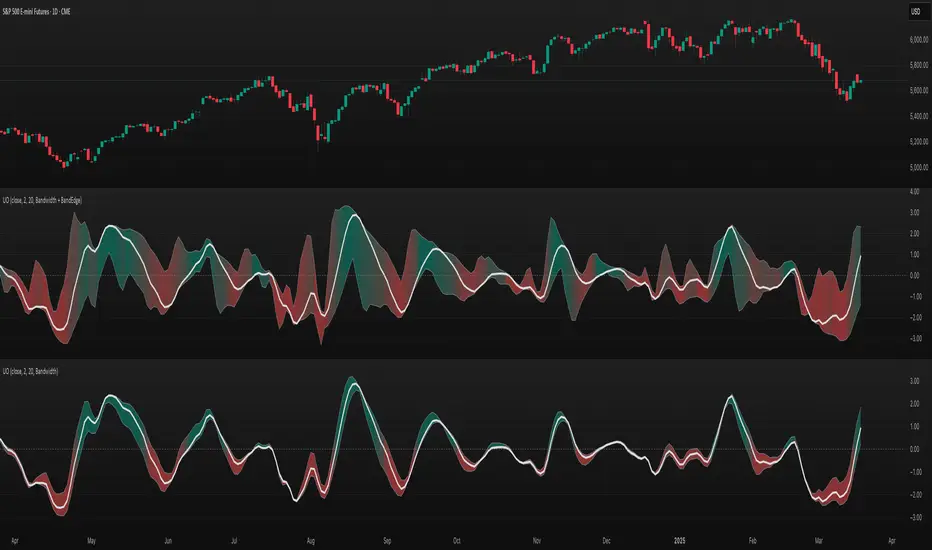
TASC 2025.04 The Ultimate Oscillator█ OVERVIEW
This script implements an alternative, refined version of the Ultimate Oscillator (UO) designed to reduce lag and enhance responsiveness in momentum indicators, as introduced by John F. Ehlers in his article "Less Lag In Momentum Indicators, The Ultimate Oscillator" from the April 2025 edition of TASC's Traders' Tips .
█ CONCEPTS
In his article, Ehlers states that indicators are essentially filters that remove unwanted noise (i.e., unnecessary information) from market data. Simply put, they process a series of data to place focus on specific information, providing a different perspective on price dynamics. Various filter types attenuate different periodic signals within the data. For instance, a lowpass filter allows only low-frequency signals, a highpass filter allows only high-frequency signals, and a bandpass filter allows signals within a specific frequency range .
Ehlers explains that the key to removing indicator lag is to combine filters of different types in such a way that the result preserves necessary, useful signals while minimizing delay (lag). His proposed UltimateOscillator aims to maintain responsiveness to a specific frequency range by measuring the difference between two highpass filters' outputs. The oscillator uses the following formula:
UO = (HP1 - HP2) / RMS
Where:
HP1 is the first highpass filter.
HP2 is another highpass filter that allows only shorter wavelengths than the critical period of HP1.
RMS is the root mean square of the highpass filter difference, used as a scaling factor to standardize the output.
The resulting oscillator is similar to a bandpass filter , because it emphasizes wavelengths between the critical periods of the two highpass filters. Ehlers' UO responds quickly to value changes in a series, providing a responsive view of momentum with little to no lag.
█ USAGE
Ehlers' UltimateOscillator sets the critical periods of its highpass filters using two parameters: BandEdge and Bandwidth :
The BandEdge sets the critical period of the second highpass filter, which determines the shortest wavelengths in the response.
The Bandwidth is a multiple of the BandEdge used for the critical period of the first highpass filter, which determines the longest wavelengths in the response. Ehlers suggests that a Bandwidth value of 2 works well for most applications. However, traders can use any value above or equal to 1.4.
Users can customize these parameters with the "Bandwidth" and "BandEdge" inputs in the "Settings/Inputs" tab.
The script plots the UO calculated for the specified "Source" series in a separate pane, with a color based on the chart's foreground color. Positive UO values indicate upward momentum or trends, and negative UO values indicate the opposite.
Additionally, this indicator provides the option to display a "cloud" from 10 additional UO series with different settings for an aggregate view of momentum. The "Cloud" input offers four display choices: "Bandwidth", "BandEdge", "Bandwidth + BandEdge", or "None".
The "Bandwidth" option calculates oscillators with different Bandwidth values based on the main oscillator's setting. Likewise, the "BandEdge" option calculates oscillators with varying BandEdge values. The "Bandwidth + BandEdge" option calculates the extra oscillators with different values for both parameters.
When a user selects any of these options, the script plots the maximum and minimum oscillator values and fills their space with a color gradient. The fill color corresponds to the net sum of each UO's sign , indicating whether most of the UOs reflect positive or negative momentum. Green hues mean most oscillators are above zero, signifying stronger upward momentum. Red hues mean most are below zero, indicating stronger downward momentum.
Mogwai Method with RSI and EMA - BTCUSD 15mThis is a custom TradingView indicator designed for trading Bitcoin (BTCUSD) on a 15-minute timeframe. It’s based on the Mogwai Method—a mean-reversion strategy—enhanced with the Relative Strength Index (RSI) for momentum confirmation. The indicator generates buy and sell signals, visualized as green and red triangle arrows on the chart, to help identify potential entry and exit points in the volatile cryptocurrency market.
Components
Bollinger Bands (BB):
Purpose: Identifies overextended price movements, signaling potential reversions to the mean.
Parameters:
Length: 20 periods (standard for mean-reversion).
Multiplier: 2.2 (slightly wider than the default 2.0 to suit BTCUSD’s volatility).
Role:
Buy signal when price drops below the lower band (oversold).
Sell signal when price rises above the upper band (overbought).
Relative Strength Index (RSI):
Purpose: Confirms momentum to filter out false signals from Bollinger Bands.
Parameters:
Length: 14 periods (classic setting, effective for crypto).
Overbought Level: 70 (price may be overextended upward).
Oversold Level: 30 (price may be overextended downward).
Role:
Buy signal requires RSI < 30 (oversold).
Sell signal requires RSI > 70 (overbought).
Exponential Moving Averages (EMAs) (Plotted but not currently in signal logic):
Purpose: Provides trend context (included in the script for visualization, optional for signal filtering).
Parameters:
Fast EMA: 9 periods (short-term trend).
Slow EMA: 50 periods (longer-term trend).
Role: Can be re-added to filter signals (e.g., buy only when Fast EMA > Slow EMA).
Signals (Triangles):
Buy Signal: Green upward triangle below the bar when price is below the lower Bollinger Band and RSI is below 30.
Sell Signal: Red downward triangle above the bar when price is above the upper Bollinger Band and RSI is above 70.
How It Works
The indicator combines Bollinger Bands and RSI to spot mean-reversion opportunities:
Buy Condition: Price breaks below the lower Bollinger Band (indicating oversold conditions), and RSI confirms this with a reading below 30.
Sell Condition: Price breaks above the upper Bollinger Band (indicating overbought conditions), and RSI confirms this with a reading above 70.
The strategy assumes that extreme price movements in BTCUSD will often revert to the mean, especially in choppy or ranging markets.
Visual Elements
Green Upward Triangles: Appear below the candlestick to indicate a buy signal.
Red Downward Triangles: Appear above the candlestick to indicate a sell signal.
Bollinger Bands: Gray lines (upper, middle, lower) plotted for reference.
EMAs: Blue (Fast) and Orange (Slow) lines for trend visualization.
How to Use the Indicator
Setup
Open TradingView:
Log into TradingView and select a BTCUSD chart from a supported exchange (e.g., Binance, Coinbase, Bitfinex).
Set Timeframe:
Switch the chart to a 15-minute timeframe (15m).
Add the Indicator:
Open the Pine Editor (bottom panel in TradingView).
Copy and paste the script provided.
Click “Add to Chart” to apply it.
Verify Display:
You should see Bollinger Bands (gray), Fast EMA (blue), Slow EMA (orange), and buy/sell triangles when conditions are met.
Trading Guidelines
Buy Signal (Green Triangle Below Bar):
What It Means: Price is oversold, potentially ready to bounce back toward the Bollinger Band middle line.
Action:
Enter a long position (buy BTCUSD).
Set a take-profit near the middle Bollinger Band (bb_middle) or a resistance level.
Place a stop-loss 1-2% below the entry (or based on ATR, e.g., ta.atr(14) * 2).
Best Context: Works well in ranging markets; avoid during strong downtrends.
Sell Signal (Red Triangle Above Bar):
What It Means: Price is overbought, potentially ready to drop back toward the middle line.
Action:
Enter a short position (sell BTCUSD) or exit a long position.
Set a take-profit near the middle Bollinger Band or a support level.
Place a stop-loss 1-2% above the entry.
Best Context: Effective in ranging markets; avoid during strong uptrends.
Trend Filter (Optional):
To reduce false signals in trending markets, you can modify the script:
Add and ema_fast > ema_slow to the buy condition (only buy in uptrends).
Add and ema_fast < ema_slow to the sell condition (only sell in downtrends).
Check the Fast EMA (blue) vs. Slow EMA (orange) alignment visually.
Tips for BTCUSD on 15-Minute Charts
Volatility: BTCUSD can be erratic. If signals are too frequent, increase bb_mult (e.g., to 2.5) or adjust RSI levels (e.g., 75/25).
Confirmation: Use volume spikes or candlestick patterns (e.g., doji, engulfing) to confirm signals.
Time of Day: Mean-reversion works best during low-volume periods (e.g., Asian session in crypto).
Backtesting: Use TradingView’s Strategy Tester (convert to a strategy by adding entry/exit logic) to evaluate performance with historical BTCUSD data up to March 13, 2025.
Risk Management
Position Size: Risk no more than 1-2% of your account per trade.
Stop Losses: Always use stops to protect against BTCUSD’s sudden moves.
Avoid Overtrading: Wait for clear signals; don’t force trades in choppy or unclear conditions.
Example Scenario
Chart: BTCUSD, 15-minute timeframe.
Buy Signal: Price drops to $58,000, below the lower Bollinger Band, RSI at 28. A green triangle appears.
Action: Buy at $58,000, target $59,000 (middle BB), stop at $57,500.
Sell Signal: Price rises to $60,500, above the upper Bollinger Band, RSI at 72. A red triangle appears.
Action: Sell at $60,500, target $59,500 (middle BB), stop at $61,000.
This indicator is tailored for mean-reversion trading on BTCUSD. Let me know if you’d like to tweak it further (e.g., add filters, alerts, or alternative indicators)!

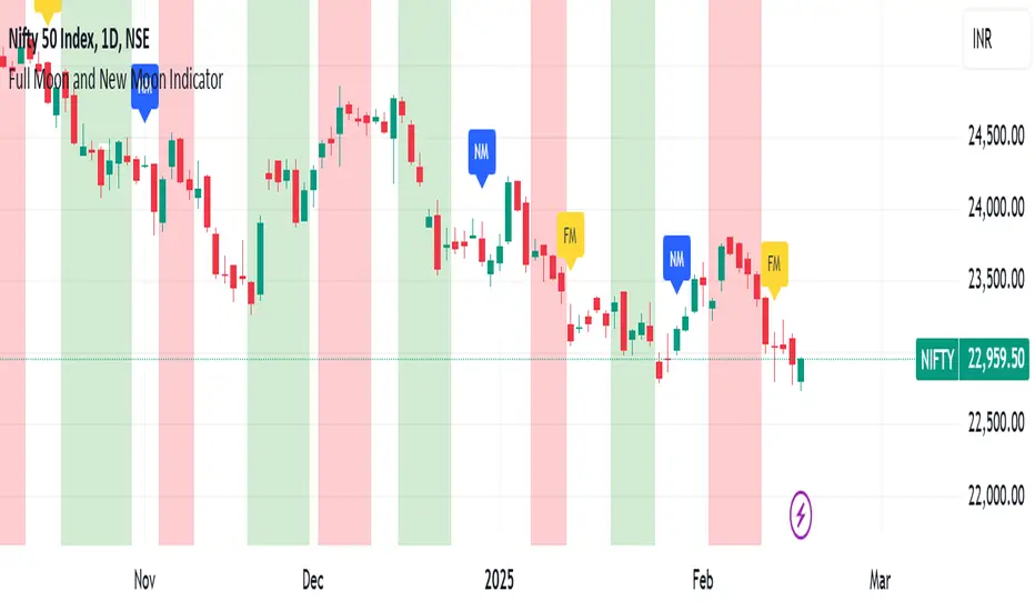
Full Moon and New Moon IndicatorThe Full Moon & New Moon Indicator is a custom Pine Script indicator which marks Full Moon (Pournami) and New Moon (Amavasya) events on the price chart. This indicator helps traders who incorporate lunar cycles into their market analysis, as certain traders believe these cycles influence market sentiment and price action. The current script is added for the year 2024 and 2025 and the dates are considered as per the Telugu calendar.
Features
✅ Identifies and labels Full Moon & New Moon days on the chart for the year 2024 and 2025
How it Works!
On a Full Moon day, it places a yellow label ("Pournami") above the corresponding candle.
On a New Moon day, it places a blue label ("Amavasya") above the corresponding candle.
Example Usage
When a Full Moon label appears, check for potential trend reversals or high volatility.
When a New Moon label appears, watch for market consolidation or a shift in sentiment.
Combine with candlestick patterns, support/resistance, or momentum indicators for a stronger trading setup.
🚀 Add this indicator to your TradingView chart and explore the market’s reaction to lunar cycles! 🌕
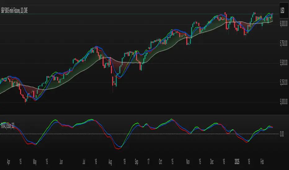
TASC 2025.03 A New Solution, Removing Moving Average Lag█ OVERVIEW
This script implements a novel technique for removing lag from a moving average, as introduced by John Ehlers in the "A New Solution, Removing Moving Average Lag" article featured in the March 2025 edition of TASC's Traders' Tips .
█ CONCEPTS
In his article, Ehlers explains that the average price in a time series represents a statistical estimate for a block of price values, where the estimate is positioned at the block's center on the time axis. In the case of a simple moving average (SMA), the calculation moves the analyzed block along the time axis and computes an average after each new sample. Because the average's position is at the center of each block, the SMA inherently lags behind price changes by half the data length.
As a solution to removing moving average lag, Ehlers proposes a new projected moving average (PMA) . The PMA smooths price data while maintaining responsiveness by calculating a projection of the average using the data's linear regression slope.
The slope of linear regression on a block of financial time series data can be expressed as the covariance between prices and sample points divided by the variance of the sample points. Ehlers derives the PMA by adding this slope across half the data length to the SMA, creating a first-order prediction that substantially reduces lag:
PMA = SMA + Slope * Length / 2
In addition, the article includes methods for calculating predictions of the PMA and the slope based on second-order and fourth-order differences. The formulas for these predictions are as follows:
PredictPMA = PMA + 0.5 * (Slope - Slope ) * Length
PredictSlope = 1.5 * Slope - 0.5 * Slope
Ehlers suggests that crossings between the predictions and the original values can help traders identify timely buy and sell signals.
█ USAGE
This indicator displays the SMA, PMA, and PMA prediction for a specified series in the main chart pane, and it shows the linear regression slope and prediction in a separate pane. Analyzing the difference between the PMA and SMA can help to identify trends. The differences between PMA or slope and its corresponding prediction can indicate turning points and potential trade opportunities.
The SMA plot uses the chart's foreground color, and the PMA and slope plots are blue by default. The plots of the predictions have a green or red hue to signify direction. Additionally, the indicator fills the space between the SMA and PMA with a green or red color gradient based on their differences:
Users can customize the source series, data length, and plot colors via the inputs in the "Settings/Inputs" tab.
█ NOTES FOR Pine Script® CODERS
The article's code implementation uses a loop to calculate all necessary sums for the slope and SMA calculations. Ported into Pine, the implementation is as follows:
pma(float src, int length) =>
float PMA = 0., float SMA = 0., float Slope = 0.
float Sx = 0.0 , float Sy = 0.0
float Sxx = 0.0 , float Syy = 0.0 , float Sxy = 0.0
for count = 1 to length
float src1 = src
Sx += count
Sy += src
Sxx += count * count
Syy += src1 * src1
Sxy += count * src1
Slope := -(length * Sxy - Sx * Sy) / (length * Sxx - Sx * Sx)
SMA := Sy / length
PMA := SMA + Slope * length / 2
However, loops in Pine can be computationally expensive, and the above loop's runtime scales directly with the specified length. Fortunately, Pine's built-in functions often eliminate the need for loops. This indicator implements the following function, which simplifies the process by using the ta.linreg() and ta.sma() functions to calculate equivalent slope and SMA values efficiently:
pma(float src, int length) =>
float Slope = ta.linreg(src, length, 0) - ta.linreg(src, length, 1)
float SMA = ta.sma(src, length)
float PMA = SMA + Slope * length * 0.5
To learn more about loop elimination in Pine, refer to this section of the User Manual's Profiling and optimization page.
TASC 2025.02 Autocorrelation Indicator█ OVERVIEW
This script implements the Autocorrelation Indicator introduced by John Ehlers in the "Drunkard's Walk: Theory And Measurement By Autocorrelation" article from the February 2025 edition of TASC's Traders' Tips . The indicator calculates the autocorrelation of a price series across several lags to construct a periodogram , which traders can use to identify market cycles, trends, and potential reversal patterns.
█ CONCEPTS
Drunkard's walk
A drunkard's walk , formally known as a random walk , is a type of stochastic process that models the evolution of a system or variable through successive random steps.
In his article, John Ehlers relates this model to market data. He discusses two first- and second-order partial differential equations, modified for discrete (non-continuous) data, that can represent solutions to the discrete random walk problem: the diffusion equation and the wave equation. According to Ehlers, market data takes on a mixture of two "modes" described by these equations. He theorizes that when "diffusion mode" is dominant, trading success is almost a matter of luck, and when "wave mode" is dominant, indicators may have improved performance.
Pink spectrum
John Ehlers explains that many recent academic studies affirm that market data has a pink spectrum , meaning the power spectral density of the data is proportional to the wavelengths it contains, like pink noise . A random walk with a pink spectrum suggests that the states of the random variable are correlated and not independent. In other words, the random variable exhibits long-range dependence with respect to previous states.
Autocorrelation function (ACF)
Autocorrelation measures the correlation of a time series with a delayed copy, or lag , of itself. The autocorrelation function (ACF) is a method that evaluates autocorrelation across a range of lags , which can help to identify patterns, trends, and cycles in stochastic market data. Analysts often use ACF to detect and characterize long-range dependence in a time series.
The Autocorrelation Indicator evaluates the ACF of market prices over a fixed range of lags, expressing the results as a color-coded heatmap representing a dynamic periodogram. Ehlers suggests the information from the periodogram can help traders identify different market behaviors, including:
Cycles : Distinguishable as repeated patterns in the periodogram.
Reversals : Indicated by sharp vertical changes in the periodogram when the indicator uses a short data length .
Trends : Indicated by increasing correlation across lags, starting with the shortest, over time.
█ USAGE
This script calculates the Autocorrelation Indicator on an input "Source" series, smoothed by Ehlers' UltimateSmoother filter, and plots several color-coded lines to represent the periodogram's information. Each line corresponds to an analyzed lag, with the shortest lag's line at the bottom of the pane. Green hues in the line indicate a positive correlation for the lag, red hues indicate a negative correlation (anticorrelation), and orange or yellow hues mean the correlation is near zero.
Because Pine has a limit on the number of plots for a single indicator, this script divides the periodogram display into three distinct ranges that cover different lags. To see the full periodogram, add three instances of this script to the chart and set the "Lag range" input for each to a different value, as demonstrated in the chart above.
With a modest autocorrelation length, such as 20 on a "1D" chart, traders can identify seasonal patterns in the price series, which can help to pinpoint cycles and moderate trends. For instance, on the daily ES1! chart above, the indicator shows repetitive, similar patterns through fall 2023 and winter 2023-2024. The green "triangular" shape rising from the zero lag baseline over different time ranges corresponds to seasonal trends in the data.
To identify turning points in the price series, Ehlers recommends using a short autocorrelation length, such as 2. With this length, users can observe sharp, sudden shifts along the vertical axis, which suggest potential turning points from upward to downward or vice versa.

Highs & Lows RTH/OVN/IBs/D/W/M/YOverview
Plots the highs and lows of RTH, OVN/ETH, IBs of those sessions, previous Day, Week, Month, and Year.
Features
Allows the user to enable/disable plotting the high/low of each period.
Lines' length, offset, and colors can be customized
Labels' position, size, color, and style can be customized
Support
Questions, feedbacks, and requests are welcomed. Please feel free to use Comments or direct private message via TradingView.
Disclaimer
This stock chart indicator provided is for informational purposes only and should not be considered as financial or investment advice. The data and information presented in this indicator are obtained from sources believed to be reliable, but we do not warrant its completeness or accuracy.
Users should be aware that:
Any investment decisions made based on this indicator are at your own risk.
The creators and providers of this indicator disclaim all liability for any losses, damages, or other consequences resulting from its use. By using this stock chart indicator, you acknowledge and accept the inherent risks associated with trading and investing in financial markets.
Release Date: 2025-01-17
Release Version: v1 r1
Release Notes Date: 2025-01-17

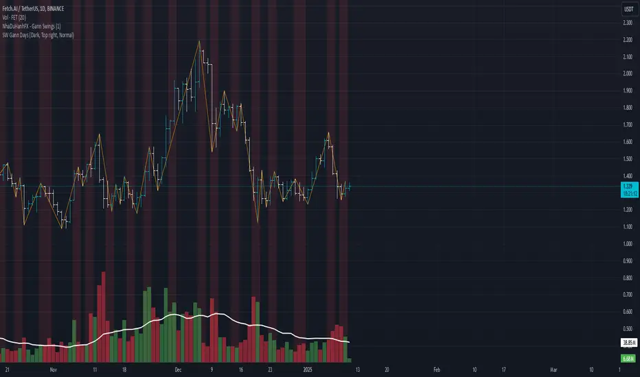
SW monthly Gann Days**Script Description:**
The script you are looking at is based on the work of W.D. Gann, a famous trader and market analyst in the early 20th century, known for his use of geometry, astrology, and numerology in market analysis. Gann believed that certain days in the market had significant importance, and he observed that markets often exhibited significant price moves around specific dates. These dates were typically associated with cyclical patterns in price movements, and Gann referred to these as "Gann Days."
In this script, we have focused on highlighting certain days of the month that Gann believed to have an influence on market behavior. The specific days in question are the **6th to 7th**, **9th to 10th**, **14th to 15th**, **19th to 20th**, **23rd to 24th**, and **29th to 31st** of each month. These ranges are based on Gann’s theory that there are recurring time cycles in the market that cause turning points or critical price movements to occur around certain days of the month.
### **Why Gann Used These Days:**
1. **Mathematical and Astrological Cycles:**
Gann believed that markets were influenced by natural cycles, and that certain dates (or combinations of dates) played a critical role in the price movements. These specific days are part of his broader theory of "time cycles" where the market would often change direction, reverse, or exhibit significant volatility on particular days. Gann's research was based on both mathematical principles and astrological observations, leading him to assign importance to these days.
2. **Gann's Universal Timing Theory:**
According to Gann, financial markets operate in a universe governed by geometric and astrological principles. These cycles repeat themselves over time, and specific days in a given month correspond to key turning points within these repeating cycles. Gann found that the 6th to 7th, 9th to 10th, 14th to 15th, 19th to 20th, 23rd to 24th, and 29th to 31st often marked significant changes in the market, making them particularly important for traders to watch.
3. **Market Psychology and Sentiment:**
These specific days likely correspond to key moments where market participants tend to react in predictable ways, influenced by past market behavior on similar dates. For example, news events or scheduled economic reports might fall within these time windows, causing the market to respond in a particular way. Gann's method involves using these cyclical patterns to predict turning points in market prices, enabling traders to anticipate when the market might make a reversal or face a significant shift in direction.
4. **Turning Points:**
Gann believed that markets often reversed or encountered critical points around specific dates. This is why he considered certain days more important than others. By identifying and focusing on these days, traders can better anticipate the market’s movement and make more informed trading decisions.
5. **Numerology:**
Gann also utilized numerology in his trading system, believing that numbers, and particularly certain key numbers, had significance in predicting market movements. The days selected in this script may correspond to numerological patterns that Gann identified in his analysis of the markets, such as recurring numbers in his astrological and geometric systems.
### **Purpose of the Script:**
This script highlights these "Gann Days" within a trading chart for 2024 and 2025. The color-coding or background highlighting is intended to draw attention to these dates, so traders can observe the potential for significant market movements during these times. By identifying these specific dates, traders following Gann's theories may gain insights into possible turning points, corrections, or key price movements based on the market's historical behavior around these days.
Overall, Gann’s use of specific days was based on his deep belief in the cyclical nature of the market and his attempt to tie those cycles to the natural laws of time, geometry, and astrology. By focusing on these dates, Gann aimed to give traders an edge in predicting significant market events and price shifts.
TASC 2025.01 Linear Predictive Filters█ OVERVIEW
This script implements a suite of tools for identifying and utilizing dominant cycles in time series data, as introduced by John Ehlers in the "Linear Predictive Filters And Instantaneous Frequency" article featured in the January 2025 edition of TASC's Traders' Tips . Dominant cycle information can help traders adapt their indicators and strategies to changing market conditions.
█ CONCEPTS
Conventional technical indicators and strategies often rely on static, unchanging parameters, which may fail to account for the dynamic nature of market data. In his article, John Ehlers applies digital signal processing principles to address this issue, introducing linear predictive filters to identify cyclic information for adapting indicators and strategies to evolving market conditions.
This approach treats market data as a complex series in the time domain. Analyzing the series in the frequency domain reveals information about its cyclic components. To reduce the impact of frequencies outside a range of interest and focus on a specific range of cycles, Ehlers applies second-order highpass and lowpass filters to the price data, which attenuate or remove wavelengths outside the desired range. This band-limited analysis isolates specific parts of the frequency spectrum for various trading styles, e.g., longer wavelengths for position trading or shorter wavelengths for swing trading.
After filtering the series to produce band-limited data, Ehlers applies a linear predictive filter to predict future values a few bars ahead. The filter, calculated based on the techniques proposed by Lloyd Griffiths, adaptively minimizes the error between the latest data point and prediction, successively adjusting its coefficients to align with the band-limited series. The filter's coefficients can then be applied to generate an adaptive estimate of the band-limited data's structure in the frequency domain and identify the dominant cycle.
█ USAGE
This script implements the following tools presented in the article:
Griffiths Predictor
This tool calculates a linear predictive filter to forecast future data points in band-limited price data. The crosses between the prediction and signal lines can provide potential trade signals.
Griffiths Spectrum
This tool calculates a partial frequency spectrum of the band-limited price data derived from the linear predictive filter's coefficients, displaying a color-coded representation of the frequency information in the pane. This mode's display represents the data as a periodogram . The bottom of each plotted bar corresponds to a specific analyzed period (inverse of frequency), and the bar's color represents the presence of that periodic cycle in the time series relative to the one with the highest presence (i.e., the dominant cycle). Warmer, brighter colors indicate a higher presence of the cycle in the series, whereas darker colors indicate a lower presence.
Griffiths Dominant Cycle
This tool compares the cyclic components within the partial spectrum and identifies the frequency with the highest power, i.e., the dominant cycle . Traders can use this dominant cycle information to tune other indicators and strategies, which may help promote better alignment with dynamic market conditions.
Notes on parameters
Bandpass boundaries:
In the article, Ehlers recommends an upper bound of 125 bars or higher to capture longer-term cycles for position trading. He recommends an upper bound of 40 bars and a lower bound of 18 bars for swing trading. If traders use smaller lower bounds, Ehlers advises a minimum of eight bars to minimize the potential effects of aliasing.
Data length:
The Griffiths predictor can use a relatively small data length, as autocorrelation diminishes rapidly with lag. However, for optimal spectrum and dominant cycle calculations, the length must match or exceed the upper bound of the bandpass filter. Ehlers recommends avoiding excessively long lengths to maintain responsiveness to shorter-term cycles.

Caja entre HorasThis script allows you to set the start time and minute you want to test and forms a “box” as the time you specified elapses. This way, you can measure volatility at market start, adjust Kill Zones to your liking, peak hours, and view H4 as a box with a colored line at the opening and another at the closing as the main box progresses, allowing you to see the fractal behavior in a shorter time frame. This helps you understand how bearish or bullish wicks are formed and at what point in the main time frame. .

ICT NY 20:00–22:00 EURUSD (Backtest en M1, 2025)//@version=5
strategy("ICT NY 20:00–22:00 EURUSD (Backtest en M15, 2024)",
overlay=true, initial_capital=10000, pyramiding=0, commission_type=strategy.commission.percent, commission_value=0.0)
// ================= Inputs =================
sessStr = input.session("2000-2200", "Sesión (NY 20:00–22:00)")
tz = input.string("America/New_York", "Zona horaria")
rr = input.float(2.0, "TP RR (1:x)", step=0.1)
slBufferPip = input.float(0.5, "Buffer SL (pips)", step=0.1)
pipSize = input.float(0.0001, "Tamaño pip EURUSD=0.0001")
onlyOneTrade = input.bool(true, "Máx. 1 trade por sesión")
// ================= Sesión =================
inSession = not na(time("", sessStr, tz))
newSession = inSession and not inSession
// Niveles de referencia: último M15 cerrado antes de 20:00
var float refHigh = na
var float refLow = na
if newSession
refHigh := high
refLow := low
// Flags de sweep
var bool sweptHigh = false
var bool sweptLow = false
if newSession
sweptHigh := false
sweptLow := false
// Sweep del último M15 antes de sesión
if inSession and not sweptHigh and not na(refHigh)
sweptHigh := high > refHigh
if inSession and not sweptLow and not na(refLow)
sweptLow := low < refLow
// ================= BOS M15 =================
breakPrevLow = close < low
breakPrevHigh = close > high
// Control de 1 trade por sesión
var int tradesThisSession = 0
if newSession
tradesThisSession := 0
canTrade = inSession and (not onlyOneTrade or tradesThisSession == 0)
// ================= Entradas =================
slBuf = slBufferPip * pipSize
if canTrade and sweptHigh and breakPrevLow
entry = close
sl = high + slBuf
risk = math.abs(entry - sl)
tp = entry - rr * risk
if sl <= entry
sl := entry + slBuf
tp := entry - rr * (sl - entry)
strategy.entry("ICT_SHORT", strategy.short, comment="Sweep High + BOS Low")
strategy.exit("TP/SL Short", from_entry="ICT_SHORT", stop=sl, limit=tp)
tradesThisSession += 1
if canTrade and sweptLow and breakPrevHigh
entry = close
sl = low - slBuf
risk = math.abs(entry - sl)
tp = entry + rr * risk
if sl >= entry
sl := entry - slBuf
tp := entry + rr * (entry - sl)
strategy.entry("ICT_LONG", strategy.long, comment="Sweep Low + BOS High")
strategy.exit("TP/SL Long", from_entry="ICT_LONG", stop=sl, limit=tp)
tradesThisSession += 1
// ================= Visuales =================
plot(inSession ? refHigh : na, "Ref High Pre-20:00", color=color.red, linewidth=2)
plot(inSession ? refLow : na, "Ref Low Pre-20:00", color=color.green, linewidth=2)
plotshape(newSession, title="Inicio Sesión NY 20:00", style=shape.flag, location=location.top, text="NY 20:00")
plotshape(sweptHigh and inSession, title="Sweep High", style=shape.triangledown, location=location.abovebar, text="Sweep High")
plotshape(sweptLow and inSession, title="Sweep Low", style=shape.triangleup, location=location.belowbar, text="Sweep Low")

Volume-MACD-RSI combined Multi-Ticker Scanner -V1 Aug 2025This scanner is adopted from a similar indicator "Volume-MACD-RSI Integrated Strategy" by Aldugrham.
The aim is to conducted automatic screening of 20 selected tickers using volume, macd and rsi and trigger alert when there is / are tickers satisfying Buy or Sell Signal, and list those tickers in the indicator pane. It can run in same time frame as the chart.

Bearish Breakaway V2 (Publish) FVG concept This is the version 2 of bearish breakaway indicator. This is the bearish version. Please also use the bullish v2 version in my page.
Here is an example, 8-15-2025, NQ,
you see the 1st 1m bearish breakaway candle formed at 941am, then you are looking for short entry, if you enter at the low of this breakaway candle, you still have enough room for a profitable trade in the short direction.
By no means, this indicator is telling to short the moment you see a bearish breakaway candle at anytime.
However, if you don't see the formation yet, it is better to not to enter the trade. It takes a lot of skills to execute the trade, how do you enter the trade based on the indicator , that will be your edge, and the indicator can only give you a visual signal.

Bullish Breakaway V2 (Publish)-FVG conceptThis is my Version 2 of the breakaway indicator based o the FVP concept.
In this version 2, I have session pre-set, ETH vs RTH, and your own session of choice ( The default setting is only for CME future product in New York timezone ).
ETH session is from 1800 to 1645.
RTH session is from 930 to 1645.
I have to end at 1645, so the data will reset at each day.
If you don't see anything on the screen, that is because you are not in an active session, so you should use replay to see the indicator.
This indicator will only work best at 1m, 5m, and 15m, if you use end time at 1645.
You may have to adjust the session time for stock product RTH vs ETH. I have not tried stock yet.
Version 2 has advanced display feature using shade, and a counter to count how many breakaway candle are in the chart.
There are several ways to use this indicator to help you trade.
In this chart 8-15-2025 NQ, you can see the 1st breakaway bullish direction formed at 1002am, if you long at 1003, you have enough space for a profitable trade in the long direction.
Notice if you even enter the low of the 2nd breakaway bullish candle, you still have room for profit in the long direction. You need to get comfortable about this trading experience. Basically you want to wait for the 1st bullish breakaway candle to form before you go for a long trade.

44 MA Near & Green Candle ScannerStocks that have closed just about 44 MA on 14th Aug 2025 and are forming green candles now

Prime NumbersPrime Numbers highlights prime numbers (no surprise there 😅), tokens and the recent "active" feature in "input".
🔸 CONCEPTS
🔹 What are Prime Numbers?
A prime number (or a prime) is a natural number greater than 1 that is not a product of two smaller natural numbers.
Wikipedia: Prime number
🔹 Prime Factorization
The fundamental theorem of arithmetic states that every integer larger than 1 can be written as a product of one or more primes. More strongly, this product is unique in the sense that any two prime factorizations of the same number will have the same number of copies of the same primes, although their ordering may differ. So, although there are many different ways of finding a factorization using an integer factorization algorithm, they all must produce the same result. Primes can thus be considered the "basic building blocks" of the natural numbers.
Wikipedia: Fundamental theorem of arithmetic
Math Is Fun: Prime Factorization
We divide a given number by Prime Numbers until only Primes remain.
Example:
24 / 2 = 12 | 24 / 3 = 8
12 / 3 = 4 | 8 / 2 = 4
4 / 2 = 2 | 4 / 2 = 2
|
24 = 2 x 3 x 2 | 24 = 3 x 2 x 2
or | or
24 = 2² x 3 | 24 = 2² x 3
In other words, every natural/integer number above 1 has a unique representation as a product of prime numbers, no matter how the number is divided. Only the order can change, but the factors (the basic elements) are always the same.
🔸 USAGE
The Prime Numbers publication contains two use cases:
Prime Factorization: performed on "close" prices, or a manual chosen number.
List Prime Numbers: shows a list of Prime Numbers.
The other two options are discussed in the DETAILS chapter:
Prime Factorization Without Arrays
Find Prime Numbers
🔹 Prime Factorization
Users can choose to perform Prime Factorization on close prices or a manually given number.
❗️ Note that this option only applies to close prices above 1, which are also rounded since Prime Factorization can only be performed on natural (integer) numbers above 1.
In the image below, the left example shows Prime Factorization performed on each close price for the latest 50 bars (which is set with "Run script only on 'Last x Bars'" -> 50).
The right example shows Prime Factorization performed on a manually given number, in this case "1,340,011". This is done only on the last bar.
When the "Source" option "close price" is chosen, one can toggle "Also current price", where both the historical and the latest current price are factored. If disabled, only historical prices are factored.
Note that, depending on the chosen options, only applicable settings are available, due to a recent feature, namely the parameter "active" in settings.
Setting the "Source" option to "Manual - Limited" will factorize any given number between 1 and 1,340,011, the latter being the highest value in the available arrays with primes.
Setting to "Manual - Not Limited" enables the user to enter a higher number. If all factors of the manual entered number are in the 1 - 1,340,011 range, these factors will be shown; however, if a factor is higher than 1,340,011, the calculation will stop, after which a warning is shown:
The calculated factors are displayed as a label where identical factors are simplified with an exponent notation in superscript.
For example 2 x 2 x 2 x 5 x 7 x 7 will be noted as 2³ x 5 x 7²
🔹 List Prime Numbers
The "List Prime Numbers" option enables users to enter a number, where the first found Prime Number is shown, together with the next x Prime Numbers ("Amount", max. 200)
The highest shown Prime Number is 1,340,011.
One can set the number of shown columns to customize the displayed numbers ("Max. columns", max. 20).
🔸 DETAILS
The Prime Numbers publication consists out of 4 parts:
Prime Factorization Without Arrays
Prime Factorization
List Prime Numbers
Find Prime Numbers
The usage of "Prime Factorization" and "List Prime Numbers" is explained above.
🔹 Prime Factorization Without Arrays
This option is only there to highlight a hurdle while performing Prime Factorization.
The basic method of Prime Factorization is to divide the base number by 2, 3, ... until the result is an integer number. Continue until the remaining number and its factors are all primes.
The division should be done by primes, but then you need to know which one is a prime.
In practice, one performs a loop from 2 to the base number.
Example:
Base_number = input.int(24)
arr = array.new()
n = Base_number
go = true
while go
for i = 2 to n
if n % i == 0
if n / i == 1
go := false
arr.push(i)
label.new(bar_index, high, str.tostring(arr))
else
arr.push(i)
n /= i
break
Small numbers won't cause issues, but when performing the calculations on, for example, 124,001 and a timeframe of, for example, 1 hour, the script will struggle and finally give a runtime error.
How to solve this?
If we use an array with only primes, we need fewer calculations since if we divide by a non-prime number, we have to divide further until all factors are primes.
I've filled arrays with prime numbers and made libraries of them. (see chapter "Find Prime Numbers" to know how these primes were found).
🔹 Tokens
A hurdle was to fill the libraries with as many prime numbers as possible.
Initially, the maximum token limit of a library was 80K.
Very recently, that limit was lifted to 100K. Kudos to the TradingView developers!
What are tokens?
Tokens are the smallest elements of a program that are meaningful to the compiler. They are also known as the fundamental building blocks of the program.
I have included a code block below the publication code (// - - - Educational (2) - - - ) which, if copied and made to a library, will contain exactly 100K tokens.
Adding more exported functions will throw a "too many tokens" error when saving the library. Subtracting 100K from the shown amount of tokens gives you the amount of used tokens for that particular function.
In that way, one can experiment with the impact of each code addition in terms of tokens.
For example adding the following code in the library:
export a() => a = array.from(1) will result in a 100,041 tokens error, in other words (100,041 - 100,000) that functions contains 41 tokens.
Some more examples, some are straightforward, others are not )
// adding these lines in one of the arrays results in x tokens
, 1 // 2 tokens
, 111, 111, 111 // 12 tokens
, 1111 // 5 tokens
, 111111111 // 10 tokens
, 1111111111111111111 // 20 tokens
, 1234567890123456789 // 20 tokens
, 1111111111111111111 + 1 // 20 tokens
, 1111111111111111111 + 8 // 20 tokens
, 1111111111111111111 + 9 // 20 tokens
, 1111111111111111111 * 1 // 20 tokens
, 1111111111111111111 * 9 // 21 tokens
, 9999999999999999999 // 21 tokens
, 1111111111111111111 * 10 // 21 tokens
, 11111111111111111110 // 21 tokens
//adding these functions to the library results in x tokens
export f() => 1 // 4 tokens
export f() => v = 1 // 4 tokens
export f() => var v = 1 // 4 tokens
export f() => var v = 1, v // 4 tokens
//adding these functions to the library results in x tokens
export a() => const arraya = array.from(1) // 42 tokens
export a() => arraya = array.from(1) // 42 tokens
export a() => a = array.from(1) // 41 tokens
export a() => array.from(1) // 32 tokens
export a() => a = array.new() // 44 tokens
export a() => a = array.new(), a.push(1) // 56 tokens
What if we could lower the amount of tokens, so we can export more Prime Numbers?
Look at this example:
829111, 829121, 829123, 829151, 829159, 829177, 829187, 829193
Eight numbers contain the same number 8291.
If we make a function that removes recurrent values, we get fewer tokens!
829111, 829121, 829123, 829151, 829159, 829177, 829187, 829193
//is transformed to:
829111, 21, 23, 51, 59, 77, 87, 93
The code block below the publication code (// - - - Educational (1) - - - ) shows how these values were reduced. With each step of 100, only the first Prime Number is shown fully.
This function could be enhanced even more to reduce recurrent thousands, tens of thousands, etc.
Using this technique enables us to export more Prime Numbers. The number of necessary libraries was reduced to half or less.
The reduced Prime Numbers are restored using the restoreValues() function, found in the library fikira/Primes_4.
🔹 Find Prime Numbers
This function is merely added to show how I filled arrays with Prime Numbers, which were, in turn, added to libraries (after reduction of recurrent values).
To know whether a number is a Prime Number, we divide the given number by values of the Primes array (Primes 2 -> max. 1,340,011). Once the division results in an integer, where the divisor is smaller than the dividend, the calculation stops since the given number is not a Prime.
When we perform these calculations in a loop, we can check whether a series of numbers is a Prime or not. Each time a number is proven not to be a Prime, the loop starts again with a higher number. Once all Primes of the array are used without the result being an integer, we have found a new Prime Number, which is added to the array.
Doing such calculations on one bar will result in a runtime error.
To solve this, the findPrimeNumbers() function remembers the index of the array. Once a limit has been reached on 1 bar (for example, the number of iterations), calculations will stop on that bar and restart on the next bar.
This spreads the workload over several bars, making it possible to continue these calculations without a runtime error.
The result is placed in log.info() , which can be copied and pasted into a hardcoded array of Prime Number values.
These settings adjust the amount of workload per bar:
Max Size: maximum size of Primes array.
Max Bars Runtime: maximum amount of bars where the function is called.
Max Numbers To Process Per Bar: maximum numbers to check on each bar, whether they are Prime Numbers.
Max Iterations Per Bar: maximum loop calculations per bar.
🔹 The End
❗️ The code and description is written without the help of an LLM, I've only used Grammarly to improve my description (without AI :) )

Intraday Volume Pulse GSK-VIZAG-AP-INDIAIntraday Volume Pulse Indicator
Overview
This indicator is designed to track and visualize intraday volume dynamics during a user-defined trading session. It calculates and displays key volume metrics such as buy volume, sell volume, cumulative delta (difference between buy and sell volumes), and total volume. The data is presented in a customizable table overlay on the chart, making it easy to monitor volume pulses throughout the session. This can help traders identify buying or selling pressure in real-time, particularly useful for intraday strategies.
The indicator resets its calculations at the start of each new day and only accumulates volume data from the specified session start time onward. It uses simple logic to classify volume as buy or sell based on candle direction:
Buy Volume: Assigned to green (up) candles or half of neutral (doji) candles.
Sell Volume: Assigned to red (down) candles or half of neutral (doji) candles.
All calculations are approximate and based on available volume data from the chart. This script does not incorporate external data sources, order flow, or tick-level information—it's purely derived from standard OHLCV (Open, High, Low, Close, Volume) bars.
Key Features
Session Customization: Define the start time of your trading session (e.g., market open) and select from common timezones like Asia/Kolkata, America/New_York, etc.
Volume Metrics:
Buy Volume: Total volume attributed to bullish activity.
Sell Volume: Total volume attributed to bearish activity.
Cumulative Delta: Net difference (Buy - Sell), highlighting overall market bias.
Total Volume: Sum of all volume during the session.
Formatted Display: Volumes are formatted for readability (e.g., in thousands "K", lakhs "L", or crores "Cr" for large numbers).
Color-Coded Table: Uses a patriotic color scheme inspired by general themes (Saffron, White, Green) with dynamic backgrounds based on positive/negative values for quick visual interpretation.
Table Options: Toggle visibility and position (top-right, top-left, etc.) for a clean chart layout.
How to Use
Add to Chart: Apply this indicator to any symbol's chart (works best on intraday timeframes like 1-min, 5-min, or 15-min).
Configure Inputs:
Session Start Hour/Minute: Set to your market's open time (default: 9:15 for Indian markets).
Timezone: Choose the appropriate timezone to align with your trading hours.
Show Table: Enable/disable the metrics table.
Table Position: Place the table where it doesn't obstruct your view.
Interpret the Table:
Monitor for spikes in buy/sell volume or shifts in cumulative delta.
Positive delta (green) suggests buying pressure; negative (red) suggests selling.
Use alongside price action or other indicators for confirmation—e.g., high total volume with positive delta could indicate bullish momentum.
Limitations:
Volume classification is heuristic and not based on actual order flow (e.g., it splits doji volume evenly).
Data accumulation starts from the session time and resets daily; historical backtesting may be limited by the max_bars_back=500 setting.
This is for educational and visualization purposes only—do not use as sole basis for trading decisions.
Calculation Details
Session Filter: Uses timestamp() to define the session start and filters bars with time >= sessionStart.
New Day Detection: Resets volumes on daily changes via ta.change(time("D")).
Volume Assignment:
Buy: Full volume if close > open; half if close == open.
Sell: Full volume if close < open; half if close == open.
Cumulative Metrics: Accumulated only during the session.
Formatting: Custom function f_format() scales large numbers for brevity.
Disclaimer
This script is for educational and informational purposes only. It does not provide financial advice or signals to buy/sell any security. Always perform your own analysis and consult a qualified financial professional before making trading decisions.
© 2025 GSK-VIZAG-AP-INDIA

Awesome Indicator# Moving Average Ribbon with ADR% - Complete Trading Indicator
## Overview
The **Moving Average Ribbon with ADR%** is a comprehensive technical analysis indicator that combines multiple analytical tools to provide traders with a complete picture of price trends, volatility, relative performance, and position sizing guidance. This multi-faceted indicator is designed for both swing and positional traders looking for data-driven entry and exit signals.
## Key Components
### 1. Moving Average Ribbon System
- **4 Customizable Moving Averages** with default periods: 13, 21, 55, and 189
- **Multiple MA Types**: SMA, EMA, SMMA (RMA), WMA, VWMA
- **Color-coded visualization** for easy trend identification
- **Flexible configuration** allowing users to modify periods, types, and colors
### 2. Average Daily Range Percentage (ADR%)
- Calculates the average daily volatility as a percentage
- Uses a 20-period simple moving average of (High/Low - 1) * 100
- Helps traders understand the stock's typical daily movement range
- Essential for position sizing and stop-loss placement
### 3. Volume Analysis (Up/Down Ratio)
- Analyzes volume distribution over the last 55 periods
- Calculates the ratio of volume on up days vs down days
- Provides insight into buying vs selling pressure
- Values > 1 indicate more buying volume, < 1 indicate more selling volume
### 4. Absolute Relative Strength (ARS)
- **Dual timeframe analysis** with customizable reference points
- **High ARS**: Performance relative to benchmark from a high reference point (default: Sep 27, 2024)
- **Low ARS**: Performance relative to benchmark from a low reference point (default: Apr 7, 2025)
- Uses NSE:NIFTY as default comparison symbol
- Color-coded display: Green for outperformance, Red for underperformance
### 5. Relative Performance Table
- **5 timeframes**: 1 Week, 1 Month, 3 Months, 6 Months, 1 Year
- Shows stock performance **relative to benchmark index**
- Formula: (Stock Return - Index Return) for each period
- **Color coding**:
- Lime: >5% outperformance
- Yellow: -5% to +5% relative performance
- Red: <-5% underperformance
### 6. Dynamic Position Allocation System
- **6-factor scoring system** based on price vs EMAs (21, 55, 189)
- Evaluates:
- Price above/below each EMA
- EMA alignment (21>55, 55>189, 21>189)
- **Allocation recommendations**:
- 100% allocation: Score = 6 (all bullish signals)
- 75% allocation: Score = 4
- 50% allocation: Score = 2
- 25% allocation: Score = 0
- 0% allocation: Score = -2, -4, -6 (bearish signals)
## Display Tables
### Performance Table (Top Right)
Shows relative performance vs benchmark across multiple timeframes with intuitive color coding for quick assessment.
### Metrics Table (Bottom Right)
Displays key statistics:
- **ADR%**: Average Daily Range percentage
- **U/D**: Up/Down volume ratio
- **Allocation%**: Recommended position size
- **High ARS%**: Relative strength from high reference
- **Low ARS%**: Relative strength from low reference
## How to Use This Indicator
### For Trend Analysis
1. **Moving Average Ribbon**: Look for price above ascending MAs for bullish trends
2. **MA Alignment**: Bullish when shorter MAs are above longer MAs
3. **Color coordination**: Use consistent color scheme for quick visual analysis
### For Entry/Exit Timing
1. **Performance Table**: Enter when showing consistent outperformance across timeframes
2. **Volume Analysis**: Confirm entries with U/D ratio > 1.5 for strong buying
3. **ARS Values**: Look for positive ARS readings for relative strength confirmation
### For Position Sizing
1. **Allocation System**: Use the recommended allocation percentage
2. **ADR% Consideration**: Adjust position size based on volatility
3. **Risk Management**: Lower allocation in high ADR% stocks
### For Risk Management
1. **ADR% for Stop Loss**: Set stops at 1-2x ADR% below entry
2. **Relative Performance**: Reduce positions when consistently underperforming
3. **Volume Confirmation**: Be cautious when U/D ratio deteriorates
## Best Practices
### Timeframe Recommendations
- **Intraday**: Use lower MA periods (5, 13, 21, 55)
- **Swing Trading**: Default settings work well (13, 21, 55, 189)
- **Position Trading**: Consider higher periods (21, 50, 100, 200)
### Market Conditions
- **Trending Markets**: Focus on MA alignment and relative performance
- **Sideways Markets**: Rely more on ADR% for range trading
- **Volatile Markets**: Reduce allocation percentage regardless of signals
### Customization Tips
1. Adjust reference dates for ARS calculation based on significant market events
2. Change comparison symbol to sector-specific indices for better relative analysis
3. Modify MA periods based on your trading style and market characteristics
## Technical Specifications
- **Version**: Pine Script v6
- **Overlay**: Yes (plots on price chart)
- **Real-time Updates**: Yes
- **Data Requirements**: Minimum 252 bars for complete calculations
- **Compatible Timeframes**: All standard timeframes
## Limitations
- Performance calculations require sufficient historical data
- ARS calculations depend on selected reference dates
- Volume analysis may be less reliable in low-volume stocks
- Relative performance is only as good as the chosen benchmark
This indicator is designed to provide a comprehensive analysis framework rather than simple buy/sell signals. It's recommended to use this in conjunction with your overall trading strategy and risk management rules.

RSI DJ GUTO 2025RSI do Samuca, tem de trocar as cores, esse e o usado nas lives, tem de trocar as cores pra ficar igual ao do Samuca pois aqui nao consegui trocar as cores.
Samuca's RSI, you have to change the colors, this is the one used in the lives, you have to change the colors to be the same as Samuca's because I couldn't change the colors here.

Supertrend EMA Vol Strategy V5### Supertrend EMA Strategy V5
**Overview**
This is a trend-following strategy designed for cryptocurrency markets like BTC/USD on daily timeframes, combining the Supertrend indicator for dynamic trailing stops with an EMA filter for trend confirmation. It aims to capture strong uptrends while avoiding counter-trend trades, with optional volume filtering for high-conviction entries and ATR-based stop-loss to manage risk. Ideal for long-only setups in bullish assets, it visually highlights trends with green/red bands and fills for easy interpretation. Backtested on BTC from 2024-2025, it shows potential for outperforming buy-and-hold in trending markets, but always use with proper risk management—past performance isn't indicative of future results.
**Key Features**
- **Supertrend Core**: Uses ATR to plot adaptive uptrend (green) and downtrend (red) lines, flipping on closes beyond prior bands for buy/sell signals.
- **EMA Trend Filter**: Entries require price above the EMA (default 21-period) for longs, ensuring alignment with the broader trend.
- **Volume Confirmation**: Optional filter only allows entries when volume exceeds its EMA (default 20-period), reducing false signals in low-activity periods.
- **Risk Controls**: Built-in ATR-multiplier stop-loss (default 2x) to cap losses; exits on Supertrend flips for trailing profits.
- **Visuals**: Green/red lines and highlighter fills for up/down trends, plus buy/sell labels and circles for signals.
- **Customizable Inputs**: Tweak ATR period (default 10), multiplier (default 3), EMA length, start date, long/short toggles, SL, and volume filter.
- **Alerts**: Built-in for buy/sell and direction changes.
**How to Use**
1. Add to your TradingView chart (e.g., BTC/USD 1D).
2. Adjust inputs: Start with defaults for trend-following; increase multiplier for fewer trades/higher win rate. Enable volume filter for volatile assets.
3. Monitor signals: Green "Buy" for long entries (if close > EMA and conditions met); red "Sell" for exits.
4. Backtest in Strategy Tester: Focus on equity curve, win rate (~50-60% in tests), and drawdown (<15% with SL).
5. Live Trading: Use small position sizes (1-2% risk per trade); combine with your analysis. Shorts disabled by default for bull-biased markets.
