Machine Learning : Torben's Moving Median KNN BandsWhat is Median Filtering ?
Median filtering is a non-linear digital filtering technique, often used to remove noise from an image or signal. Such noise reduction is a typical pre-processing step to improve the results of later processing (for example, edge detection on an image). Median filtering is very widely used in digital image processing because, under certain conditions, it preserves edges while removing noise (but see the discussion below), also having applications in signal processing.
The main idea of the median filter is to run through the signal entry by entry, replacing each entry with the median of neighboring entries. The pattern of neighbors is called the "window", which slides, entry by entry, over the entire signal. For one-dimensional signals, the most obvious window is just the first few preceding and following entries, whereas for two-dimensional (or higher-dimensional) data the window must include all entries within a given radius or ellipsoidal region (i.e. the median filter is not a separable filter).
The median filter works by taking the median of all the pixels in a neighborhood around the current pixel. The median is the middle value in a sorted list of numbers. This means that the median filter is not sensitive to the order of the pixels in the neighborhood, and it is not affected by outliers (very high or very low values).
The median filter is a very effective way to remove noise from images. It can remove both salt and pepper noise (random white and black pixels) and Gaussian noise (randomly distributed pixels with a Gaussian distribution). The median filter is also very good at preserving edges, which is why it is often used as a pre-processing step for edge detection.
However, the median filter can also blur images. This is because the median filter replaces each pixel with the value of the median of its neighbors. This can cause the edges of objects in the image to be smoothed out. The amount of blurring depends on the size of the window used by the median filter. A larger window will blur more than a smaller window.
The median filter is a very versatile tool that can be used for a variety of tasks in image processing. It is a good choice for removing noise and preserving edges, but it can also blur images. The best way to use the median filter is to experiment with different window sizes to find the setting that produces the desired results.
What is this Indicator ?
K-nearest neighbors (KNN) is a simple, non-parametric machine learning algorithm that can be used for both classification and regression tasks. The basic idea behind KNN is to find the K most similar data points to a new data point and then use the labels of those K data points to predict the label of the new data point.
Torben's moving median is a variation of the median filter that is used to remove noise from images. The median filter works by replacing each pixel in an image with the median of its neighbors. Torben's moving median works in a similar way, but it also averages the values of the neighbors. This helps to reduce the amount of blurring that can occur with the median filter.
KNN over Torben's moving median is a hybrid algorithm that combines the strengths of both KNN and Torben's moving median. KNN is able to learn the underlying distribution of the data, while Torben's moving median is able to remove noise from the data. This combination can lead to better performance than either algorithm on its own.
To implement KNN over Torben's moving median, we first need to choose a value for K. The value of K controls how many neighbors are used to predict the label of a new data point. A larger value of K will make the algorithm more robust to noise, but it will also make the algorithm less sensitive to local variations in the data.
Once we have chosen a value for K, we need to train the algorithm on a dataset of labeled data points. The training dataset will be used to learn the underlying distribution of the data.
Once the algorithm is trained, we can use it to predict the labels of new data points. To do this, we first need to find the K most similar data points to the new data point. We can then use the labels of those K data points to predict the label of the new data point.
KNN over Torben's moving median is a simple, yet powerful algorithm that can be used for a variety of tasks. It is particularly well-suited for tasks where the data is noisy or where the underlying distribution of the data is unknown.
Here are some of the advantages of using KNN over Torben's moving median:
KNN is able to learn the underlying distribution of the data.
KNN is robust to noise.
KNN is not sensitive to local variations in the data.
Here are some of the disadvantages of using KNN over Torben's moving median:
KNN can be computationally expensive for large datasets.
KNN can be sensitive to the choice of K.
KNN can be slow to train.
Cari dalam skrip untuk "如何用wind搜索股票的发行价和份数"

[blackcat] L2 Ehlers FilterLevel: 2
Background
John F. Ehlers introuced Ehlers Filter in his "Rocket Science for Traders" chapter 18 on 2001.
Function
blackcat L2 Ehlers Filter is used to follow trend. The filters Dr. Ehlers have invented are nonlinear FIR filters. It turns out that they provide both extraordinary smoothing in sideways markets and aggressively follow major price movements with minimal lag. The development of Ehlers filters starts with a general
class of FIR filters called Order Statistic (OS) filters. These filters are well-known for speech and image processing, to sharpen edges, increase contrast, and for robust estimation. In contrast to linear filters, where temporal ordering of the samples is preserved, OS filters base their operation on the ranking of samples
within the filter window. The data are ranked by their summary statistics, such as their mean or variance, rather than by their temporal position.
Among OS filters, the Median filter is the best known. In a Median filter, the output is the median value of all the data values within the observation window. As opposed to an averaging filter, the Median filter simply discards all data except the median value. In this way, impulsive noise spikes and extreme price data are eliminated rather than included in the average. The median value can fall at the first sample in the data window, at the last sample, or anywhere in between. Thus, temporal characteristics are lost. The Median filter tends to smooth out short-term variations that lead to whipsaw trades with linear filters. However, the lag of a Median filter in response to a sharp and sustained price movement is substantial --- it necessarily is about half the filter window width.
Key Signal
Coef --> Ehlers filter coefficients array
Filt --> Ehlers filter output
Pros and Cons
100% John F. Ehlers definition translation of original work, even variable names are the same. This help readers who would like to use pine to read his book. If you had read his works, then you will be quite familiar with my code style.
Remarks
The 14th script for Blackcat1402 John F. Ehlers Week publication.
Readme
In real life, I am a prolific inventor. I have successfully applied for more than 60 international and regional patents in the past 12 years. But in the past two years or so, I have tried to transfer my creativity to the development of trading strategies. Tradingview is the ideal platform for me. I am selecting and contributing some of the hundreds of scripts to publish in Tradingview community. Welcome everyone to interact with me to discuss these interesting pine scripts.
The scripts posted are categorized into 5 levels according to my efforts or manhours put into these works.
Level 1 : interesting script snippets or distinctive improvement from classic indicators or strategy. Level 1 scripts can usually appear in more complex indicators as a function module or element.
Level 2 : composite indicator/strategy. By selecting or combining several independent or dependent functions or sub indicators in proper way, the composite script exhibits a resonance phenomenon which can filter out noise or fake trading signal to enhance trading confidence level.
Level 3 : comprehensive indicator/strategy. They are simple trading systems based on my strategies. They are commonly containing several or all of entry signal, close signal, stop loss, take profit, re-entry, risk management, and position sizing techniques. Even some interesting fundamental and mass psychological aspects are incorporated.
Level 4 : script snippets or functions that do not disclose source code. Interesting element that can reveal market laws and work as raw material for indicators and strategies. If you find Level 1~2 scripts are helpful, Level 4 is a private version that took me far more efforts to develop.
Level 5 : indicator/strategy that do not disclose source code. private version of Level 3 script with my accumulated script processing skills or a large number of custom functions. I had a private function library built in past two years. Level 5 scripts use many of them to achieve private trading strategy.
Unchased Wick Detector and ReversalsThis indicator can be used to track unchased wick from previous pivot points.
The idea is to visualise liquidity cluster and grab before a potential reversal.
Unchased wick Visual:
- White lines are protected highs or lows.
- Gray lines are previous wicks where prices have passed through and where the prices did not reverse.
Reversal window:
Reversal window parameters define a period range (a min and a max bars) where the reversal is valid.
The idea is that the reversal must be done in the couple bars right after the wick is chased (this event should stay short in time but you can adjust the period as you wish).
By default the default, the window 1-5 bars (e.g., daily, during 1-5 days).
Green color indicates a grab from a low and a reversal to the upside.
Red color indicates a grab from a high and a reversal to the downside.
Disclamer:
Of course this indicator can lead to false reversal signals and must be combined with other data and must be careful to use it alone for opening any position.
This indicator is a Alpha version let me know if any problem.

ORB_RDORB_RD - Opening Range Box (Ryan DeBraal)
This indicator automatically draws a high/low box for the first portion of
each trading day, automatically stepping the range window from 15, 30, 45,
up to 60 minutes after the session starts. The box updates live as the range
forms, then optionally extends across the rest of the session.
FEATURES
-----------------------------------------------------------------------------
• Opening Range Detection
- Automatically ladders the range window: 0–15, 0–30, 0–45, 0–60 minutes
- Automatic reset at each new trading day
- Live high/low updates while inside the 0–60 minute window
• Auto-Drawing Range Box
- Draws a dynamic rectangle as the range forms
- Top and bottom update with every new high/low
- Extends sideways in real time during formation
- Optional full-day extension after the 60-minute range finalizes
• Customizable Visuals
- Adjustable fill transparency
- Mild green tint by default for clarity
PURPOSE
-----------------------------------------------------------------------------
This tool highlights the evolving opening range, a widely used intraday
reference for breakout traders, mean-reversion setups, and session structure
analysis. Ideal for:
• Identifying early support and resistance
• Framing breakout and pullback decisions
• Tracking intraday trend bias after the morning range

Weighted KDE Mode🙏🏻 The ‘ultimate’ typical value estimator, for the highest computational cost @ time complexity O(n^2). I am not afraid to say: this is the last resort BFG9000 you can ‘ever’ get to make dem market demons kneel before y’all
Quickguide
pls read it, you won’t find it anywhere else in open access
When to use:
If current market activity is so crazy || things on your charts are really so bad (contaminated data && (data has very heavy tails || very pronounced peak)), the only option left is to use the peak (mode) of Kernel Density Estimate , instead of median not even mentioning mean. So when WMA won’t help, when WPNR won’t help, you need this thing.
Setting it up:
Interval: choose what u need, you can use usual moving windows, but I also added yearly and session anchors alike in old VWAP (always prefer 24h instead of Session if your plan allows). Other options like cumulative window are also there.
Parameters: this script ain't no joke, it needs time to make calculations, so I added a setting to calculate only for the last N bars (when “starting at bar N” is put on 0). If it’s not zero it acts as a starting point after which the calculations happen (useful for backtesting). Other parameters keep em as they are, keep student5 kernel , turn off appropriate weights if u apply it to other than chart data, on other studies etc.
But instead of listening to me just experiment with parameters and see what they change, would take 5 mins max
Been always saying that VWAP is ish, not time-aware etc, volume info is incorporated in a lil bit wrong way… So I decided not just to fix VWAP (you can do it yourself in 5 mins), but instead to drop there the Ultimate xD typical value estimator that is ever possible to do. Time aware, volume / inferred volume aware, resistant to all kinds of BS. This is your shieldwall.
How it works:
You can easily do a weighted kernel density estimation, in our case including temporal and intensity information while accumulating densities. Here are some details worth mentioning about the thing:
Kernels are raw (not unit variance), that’s easier to work with later.
h_constants for each kernel were calculated ^^ given that ^^ with python mpmath module with high decimal precision.
In bandwidth calculation instead of using empirical standard deviation as a scaler, I use... ta.range(src, len) / math.sqrt(12)
...that takes data range and converts it to standard deviation, assuming data is uniformly distributed. That’s exactly what we need: a scaler that is coherent with the KDE, that has nothing to do with stdevs, as the kernels except for gaussian ones (that we don’t even need to use). More importantly, if u take multiple windows and see over time which distro they approach on the long term, that would be the uniform one (not the normal one as many think). Sometimes windows are multimodal, sometimes Laplace like etc, so in general all together they are uniform ish.
The one and only kernel you really need is Student t with v = 5 , for the use case I highlighted in the first part of the post for TV users. It’s as far as u can get until ish becomes crazy like undefined variance etc. It has the highest kurtosis = 9 of all distros, perfect for the real use case I mentioned. Otherwise, you don’t even need KDE 4 real, but still I included other senseful kernels for comparison or in case I am trippin there.
Btw, don’t believe in all that hype about Epanechnikov kernel which in essence is made from beta distribution with alpha = beta = 2, idk why folk call it with that weird name, it’s beta2 kernel. Yes on papers it really minimises AMISE (that’s how I calculated h constants for all dem kernels in the script), but for really crazy data (proper use case for us), it ain't provides even ‘closely’ compared with student5 kernel. Not much else to add.
Shout out to @RicardoSantos for inspiration, I saw your KDE script a long time ago brotha, finna got my hands on it.
∞

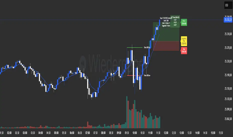
Morning ORB FVG Trigger✅ Overview
Morning ORB FVG Trigger is a complete intraday trading framework built around:
A Morning Opening Range Breakout (ORB)
The first Fair Value Gap (FVG) after that breakout
Strict risk management and position sizing
Optional HTF trend filter (Daily / Weekly / Monthly)
Optional Daily ATR filter to avoid extreme days
The script is designed for futures / indices / FX on intraday charts up to 15 minutes and for traders who want a clean, mechanical entry framework with clear risk.
🧠 Core idea
Define a morning opening range (e.g. 09:30–09:45).
Wait for a clean breakout above/below that range.
After the breakout, wait for the first FVG in breakout direction,
confirmed by the next candle (no immediate full reclaim).
Use a chosen stop logic + R:R factor to build risk/reward boxes.
Calculate position size based on your account risk.
(Optional) Only take trades:
In the direction of the HTF EMA trend (D/W/M).
On days where the morning range is within a band of the Daily ATR.
You can also disable all signals/boxes and use the script just as a visual ORB tool.
⏰ 1. ORB / Morning Range
Inputs (Main section)
Morning Range Session
Time window of the opening range in exchange time
Example: 09:30–09:45 for a 15-minute ORB.
You can type custom ranges (e.g. 09:30–09:35 for a 5-minute ORB).
Risk/Reward (TP factor)
Multiplier for the take-profit distance relative to the stop.
2.0 = TP is 2× the stop distance
1.5 = TP is 1.5× the stop distance
Show ORB range
If enabled, draws:
ORB high/low lines
ORB labels (e.g. 15min ORB high / low)
Optional midline
Extend ORB lines to the right (bars)
How many bars to extend the ORB high/low horizontally beyond the ORB itself.
Trade box width (bars)
Horizontal width (in bars) of:
Red risk box (entry–stop)
Green reward box (entry–TP)
Implementation details
The ORB is always calculated on 1-minute data internally, so it stays precise even on 5m/15m charts.
The script only works on intraday timeframes up to 15 minutes.
📦 2. FVG Block
Group: “FVG”
Threshold %
Minimum size of an FVG in % of price.
0 = every FVG
Higher values = only larger gaps
Auto threshold (from volatility)
If enabled, the minimum FVG size is derived from historical volatility
instead of a fixed percentage.
Allow breakout FVG partly inside ORB
Off (default): the FVG must lie fully outside the ORB.
On: the breakout FVG itself may still overlap the ORB a bit,
as long as it is the first one attached to the breakout move.
Enable FVG entry signals, boxes & alerts
On: full system – FVG detection, entry labels, risk/TP boxes, alerts.
Off: no entries, no risk/TP boxes, no alerts.
You only get the ORB and (optionally) the HTF dashboard, so you can trade your own setups.
Entry mode
Entry mode (Mid / Edge / NextOpen)
Mid – Entry at the midpoint of the FVG.
Edge – Long at the upper FVG edge, short at the lower FVG edge.
NextOpen – No limit order in the gap. Entry is placed at the next bar open after FVG confirmation.
Edge offset (ticks)
Additional offset for Edge entries:
Long:
+ticks = a bit above the FVG (more conservative)
-ticks = deeper into the FVG (more aggressive)
Short:
+ticks = a bit below the FVG
-ticks = deeper into the FVG
FVG detection logic
Uses a LuxAlgo-style 3-candle FVG pattern (gap between candle 1 and 3).
Only one FVG is taken: the first valid FVG after the ORB breakout in breakup direction.
The FVG candle is the middle bar; the script:
Detects the FVG on the previous bar.
Waits for the current bar to confirm it:
Bullish: current low must stay above the lower FVG boundary
Bearish: current high must stay below the upper FVG boundary
Only then an entry signal is generated.
🛑 3. Stop Logic
Group: “Stop Logic”
Stop mode (PrevBar / Pivot / FVG Candle)
PrevBar – Stop at the low/high of the candle before the FVG
(tight/aggressive).
FVG Candle – Stop at the low/high of the FVG candle itself
(medium).
Pivot – Stop at the most recent swing high/low
using pivotLeft / pivotRight pivots (more conservative).
Ticks (stop buffer)
Offset (in ticks) from the selected stop level.
> 0 = further away (more room, more risk)
< 0 = closer (tighter stop)
Pivot left / Pivot right
Number of candles left/right to define a swing high/low
when using Pivot stop mode.
Typical intraday values: 2–3.
The script also sanity-checks the stop:
if the calculated stop would be invalid (e.g. above entry in a long), it moves it by a minimal distance (2 ticks) to keep a valid risk.
📈 4. HTF Trend Filter (Daily / Weekly / Monthly)
Group: “HTF Trend Filter”
Enable HTF trend filter
If enabled, trades are only allowed:
Long when at least 2 of D/W/M closes are above their EMA
Short when at least 2 of D/W/M closes are below their EMA
EMA length (D/W/M)
EMA length for all three higher timeframes (Daily, Weekly, Monthly).
This helps focus entries in the direction of the dominant higher-timeframe trend.
📊 5. ATR Filter (Daily)
Group: “ATR Filter (Daily)”
Use daily ATR filter
If enabled, the height of the ORB (ORB high – ORB low) must be within
a band of the Daily ATR to allow any signals.
Daily ATR length
ATR period on the Daily timeframe.
Min ORB size vs ATR
Lower bound:
Example: 0.3 → ORB must be at least 0.3 × Daily ATR
0.0 = no minimum.
Max ORB size vs ATR
Upper bound:
Example: 1.5 → ORB must be ≤ 1.5 × Daily ATR
0.0 = no maximum.
If the ORB is too small (choppy) or too large (exhausted move), no breakout or FVG signal will be generated on that day.
🧭 6. HTF Dashboard & Signal Labels
Group: “HTF Trend Dashboard”
Show HTF dashboard
Draws a small label at the top of the chart showing:
HTF Trend (EMA X)
D: UP/FLAT/DOWN
W: UP/FLAT/DOWN
M: UP/FLAT/DOWN
Dashboard position
Top Right, Top Center, Top Left – places the dashboard at the top.
Over Risk Info – no top dashboard; instead, the HTF trend info is shown as a label near the risk box when a new signal appears.
Lookback (bars) for top anchor
How many bars to use to determine the top price level for dashboard placement.
Show HTF trend above risk box on signal
Only relevant if Dashboard position = Over Risk Info.
When enabled, a small HTF label appears near the risk box for each new trade.
Signal label vertical offset (ticks)
Vertical spacing between risk info label and HTF label.
Minimum spacing HTF/Risk (ticks)
Ensures a minimum vertical distance so the two labels don’t overlap.
HTF signal label X offset (bars)
Horizontal offset (left/right) relative to the risk info label.
⏳ 7. ORB–FVG Filters (Session & Time Window)
Group: “ORB FVG Filter”
Only same session day
If enabled, FVG entries are only allowed on the same calendar day
as the ORB. When the date changes, all state & drawings are reset.
Limit hours after ORB
Enables a time window after the ORB end.
Trading window after ORB (hours)
Length of that window in hours.
Example: 2.0 → FVG signals only in the first 2 hours after ORB end.
💰 8. Risk Management & Position Sizing
Group: “Risk Management”
Calculate position size
If enabled, the script computes suggested mini and micro contract size for you.
Account size
Your trading account size (in account currency).
Risk mode
Percent – risk is a % of account size (Account risk %).
Fixed amount – risk is a fixed dollar amount (Fixed risk ($)).
Account risk %
Risk per trade as a percentage of account size (e.g. 1.0 for 1%).
Fixed risk ($)
Fixed risk per trade in dollars when using Fixed amount mode.
Micro factor (vs mini)
How much a micro contract is worth relative to a mini.
Example:
0.1 → one micro moves 1/10 of one mini.
Risk Info label
For each new trade, a label is shown above the boxes with:
Stop distance in price and $ risk per mini
Max risk allowed for the trade
Suggested mini and micro size
Text like:
Suggested: 2 mini
Suggested: 5 micro
or Suggested: no trade
This makes the script especially useful for prop-firm rules or strict risk discipline.
🎨 9. Visual Style (Boxes, Labels, ORB Lines)
Group: “Box & Label Style (Trade)”
Label font size (Very small, Small, Normal, Large)
Entry label BG / text color
Stop label BG / text color
TP label BG / text color
Risk info BG / text color
Risk box color (entry–stop zone)
Reward box color (entry–TP zone)
Group: “ORB Style”
ORB high line color
ORB low line color
ORB line width
ORB label font size
ORB label background color
ORB label text color
Show ORB midline
ORB midline color / width / style (Solid / Dashed / Dotted)
⚠️ 10. Alerts
Group: “Alerts”
The script defines three alert conditions:
Long entry FVG breakout
Triggered when a new long signal appears.
Short entry FVG breakout
Triggered when a new short signal appears.
FVG entry (long/short)
Generic alert for any new signal (long or short).
To use them:
Add the indicator to the chart.
Open the Alerts dialog → “Condition”.
Select this script and one of the alert conditions.
Set your preferred expiration and notification settings.
Alerts only fire when Enable FVG entry signals, boxes & alerts is on.
🧩 11. How the trading logic flows (summary)
Build ORB on 1-minute data during the selected session.
Optionally reject the day if ORB is outside the ATR bounds.
Wait for a breakout (close above high or below low), respecting HTF trend filter.
After breakout, look for the first valid FVG in that direction:
Outside the ORB (unless breakout FVG allowed inside)
Confirmed by the next candle (no full reclaim)
Once confirmed:
Compute entry, stop, target.
Draw risk/reward boxes and all labels.
Optionally show HTF signal label over the risk info.
Trigger alerts if enabled.
If you disable FVG signals, only steps 1–3 (plus dashboard) are effectively active.
⚠️ 12. Notes & Disclaimer
Script is intended for intraday trading up to 15-minute timeframes.
All signals are mechanical and do not guarantee profitability.
Always backtest and forward-test on your own data before risking real money.
This script is for educational purposes only and is not financial advice.
🚀 Quick-start guide
Add the script to your chart
Use an intraday timeframe ≤ 15 minutes (1m, 3m, 5m, 15m).
Works best on liquid indices, futures, FX and large-cap stocks.
Set the Morning Range
In “Morning Range Session” choose the exchange’s opening window.
Examples
US index futures (CME): 08:30–08:45 or 08:30–08:35
US stocks (NYSE/Nasdaq): 09:30–09:45 or 09:30–09:35
The ORB is always calculated on 1-minute data internally, so the range stays accurate on higher intraday charts.
Keep the default filters at first
HTF Trend Filter: ON
EMA length = 20
This will only allow trades in the direction of the dominant D/W/M trend.
ATR Filter: OFF (optional; you can enable later once you’re comfortable).
Use the full trade system
In the FVG group leave
“Enable FVG entry signals, boxes & alerts” = ON
Entry mode: Mid
Stop mode: FVG Candle or PrevBar
Risk/Reward: 2.0 as a starting point.
Set your risk
Turn on “Calculate position size”.
Enter your Account size and choose either:
Risk mode = Percent (e.g. 1.0 = 1% per trade), or
Risk mode = Fixed amount (e.g. $250 per trade).
The risk info label will show:
Stop distance in price and $/contract
Max allowed risk
Suggested mini and micro contract size.
Enable alerts (optional)
Open the Alerts dialog → Condition: this script.
Choose one of:
Long entry FVG breakout
Short entry FVG breakout
FVG entry (long/short)
Choose “Once per bar” or “Once per bar close”, and your preferred notification type.
Replay & journal
Use the TradingView bar replay tool to step through past days.
Focus on:
How the ORB defines the structure.
How the first confirmed FVG outside the ORB behaves.
Whether the risk/TP levels fit your own style and product.
🎛 Recommended settings & profiles
These are starting points, not rules. Always adapt to the instrument and your own risk tolerance.
1. Conservative / Trend-following
Timeframe: 5m or 15m
Morning Range Session: 15-minute ORB around the cash or futures open
FVG
Threshold %: 0.05–0.1 (filter out very small gaps)
Auto threshold: OFF (keep it simple)
Allow breakout FVG partly inside ORB: OFF
Enable FVG entry signals/boxes/alerts: ON
Entry mode: Mid
Stop Logic
Stop mode: Pivot
Pivot left/right: 2–3
Stop buffer: +1–2 ticks
HTF Trend Filter
Enabled: ON
EMA length: 20
ATR Filter
Enabled: ON
Daily ATR length: 14
Min ORB vs ATR: 0.3–0.4
Max ORB vs ATR: 1.2–1.5
Risk Management
Risk mode: Percent
Account risk: 0.5–1.0%
Idea: Only trade when the higher-timeframe trend supports the move and the opening range is of a “normal” size for the current volatility.
2. Balanced / Intraday directional
Timeframe: 3m or 5m
FVG
Threshold %: 0.02–0.05
Auto threshold: ON (lets the script adapt to volatility)
Allow breakout FVG partly inside ORB: ON
(first breakout FVG may partly sit inside the ORB)
Entry mode: Edge
Edge offset (ticks): 0 or +1
Stop Logic
Stop mode: FVG Candle
Stop buffer: 0–1 ticks
HTF Trend Filter
Enabled: ON
ATR Filter
Enabled: OFF (optional)
Risk Management
Risk mode: Percent
Account risk: 1.0–1.5% (if this fits your plan)
Idea: Slightly more aggressive entries at the gap edge, still aligned with HTF trend, but with more flexibility on ATR.
3. Aggressive / Scalping around the ORB
Timeframe: 1m or 3m
FVG
Threshold %: 0.0–0.02
Auto threshold: ON
Allow breakout FVG partly inside ORB: ON
Entry mode: NextOpen or Edge with a negative offset (deeper into the gap)
Stop Logic
Stop mode: PrevBar
Stop buffer: 0 or -1 tick
HTF Trend Filter
Enabled: OFF (or ON but treat as soft guidance)
ATR Filter
Enabled: OFF
Risk Management
Risk mode: Percent
Account risk: lower, e.g. 0.25–0.5% per trade
Idea: More trades and tighter stops. Best for experienced traders who understand the limitations of scalping and whipsaw risk.
Final reminder
All of these are templates, not guarantees:
Always check how the system behaves on your market and session.
Start on replay and demo before trading real money.
Adjust filters (HTF, ATR, thresholds) until the signals fit your personal approach.
Algorithm Predator - ML-liteAlgorithm Predator - ML-lite
This indicator combines four specialized trading agents with an adaptive multi-armed bandit selection system to identify high-probability trade setups. It is designed for swing and intraday traders who want systematic signal generation based on institutional order flow patterns , momentum exhaustion , liquidity dynamics , and statistical mean reversion .
Core Architecture
Why These Components Are Combined:
The script addresses a fundamental challenge in algorithmic trading: no single detection method works consistently across all market conditions. By deploying four independent agents and using reinforcement learning algorithms to select or blend their outputs, the system adapts to changing market regimes without manual intervention.
The Four Trading Agents
1. Spoofing Detector Agent 🎭
Detects iceberg orders through persistent volume at similar price levels over 5 bars
Identifies spoofing patterns via asymmetric wick analysis (wicks exceeding 60% of bar range with volume >1.8× average)
Monitors order clustering using simplified Hawkes process intensity tracking (exponential decay model)
Signal Logic: Contrarian—fades false breakouts caused by institutional manipulation
Best Markets: Consolidations, institutional trading windows, low-liquidity hours
2. Exhaustion Detector Agent ⚡
Calculates RSI divergence between price movement and momentum indicator over 5-bar window
Detects VWAP exhaustion (price at 2σ bands with declining volume)
Uses VPIN reversals (volume-based toxic flow dissipation) to identify momentum failure
Signal Logic: Counter-trend—enters when momentum extreme shows weakness
Best Markets: Trending markets reaching climax points, over-extended moves
3. Liquidity Void Detector Agent 💧
Measures Bollinger Band squeeze (width <60% of 50-period average)
Identifies stop hunts via 20-bar high/low penetration with immediate reversal and volume spike
Detects hidden liquidity absorption (volume >2× average with range <0.3× ATR)
Signal Logic: Breakout anticipation—enters after liquidity grab but before main move
Best Markets: Range-bound pre-breakout, volatility compression zones
4. Mean Reversion Agent 📊
Calculates price z-scores relative to 50-period SMA and standard deviation (triggers at ±2σ)
Implements Ornstein-Uhlenbeck process scoring (mean-reverting stochastic model)
Uses entropy analysis to detect algorithmic trading patterns (low entropy <0.25 = high predictability)
Signal Logic: Statistical reversion—enters when price deviates significantly from statistical equilibrium
Best Markets: Range-bound, low-volatility, algorithmically-dominated instruments
Adaptive Selection: Multi-Armed Bandit System
The script implements four reinforcement learning algorithms to dynamically select or blend agents based on performance:
Thompson Sampling (Default - Recommended):
Uses Bayesian inference with beta distributions (tracks alpha/beta parameters per agent)
Balances exploration (trying underused agents) vs. exploitation (using proven winners)
Each agent's win/loss history informs its selection probability
Lite Approximation: Uses pseudo-random sampling from price/volume noise instead of true random number generation
UCB1 (Upper Confidence Bound):
Calculates confidence intervals using: average_reward + sqrt(2 × ln(total_pulls) / agent_pulls)
Deterministic algorithm favoring agents with high uncertainty (potential upside)
More conservative than Thompson Sampling
Epsilon-Greedy:
Exploits best-performing agent (1-ε)% of the time
Explores randomly ε% of the time (default 10%, configurable 1-50%)
Simple, transparent, easily tuned via epsilon parameter
Gradient Bandit:
Uses softmax probability distribution over agent preference weights
Updates weights via gradient ascent based on rewards
Best for Blend mode where all agents contribute
Selection Modes:
Switch Mode: Uses only the selected agent's signal (clean, decisive)
Blend Mode: Combines all agents using exponentially weighted confidence scores controlled by temperature parameter (smooth, diversified)
Lock Agent Feature:
Optional manual override to force one specific agent
Useful after identifying which agent dominates your specific instrument
Only applies in Switch mode
Four choices: Spoofing Detector, Exhaustion Detector, Liquidity Void, Mean Reversion
Memory System
Dual-Layer Architecture:
Short-Term Memory: Stores last 20 trade outcomes per agent (configurable 10-50)
Long-Term Memory: Stores episode averages when short-term reaches transfer threshold (configurable 5-20 bars)
Memory Boost Mechanism: Recent performance modulates agent scores by up to ±20%
Episode Transfer: When an agent accumulates sufficient results, averages are condensed into long-term storage
Persistence: Manual restoration of learned parameters via input fields (alpha, beta, weights, microstructure thresholds)
How Memory Works:
Agent generates signal → outcome tracked after 8 bars (performance horizon)
Result stored in short-term memory (win = 1.0, loss = 0.0)
Short-term average influences agent's future scores (positive feedback loop)
After threshold met (default 10 results), episode averaged into long-term storage
Long-term patterns (weighted 30%) + short-term patterns (weighted 70%) = total memory boost
Market Microstructure Analysis
These advanced metrics quantify institutional order flow dynamics:
Order Flow Toxicity (Simplified VPIN):
Measures buy/sell volume imbalance over 20 bars: |buy_vol - sell_vol| / (buy_vol + sell_vol)
Detects informed trading activity (institutional players with non-public information)
Values >0.4 indicate "toxic flow" (informed traders active)
Lite Approximation: Uses simple open/close heuristic instead of tick-by-tick trade classification
Price Impact Analysis (Simplified Kyle's Lambda):
Measures market impact efficiency: |price_change_10| / sqrt(volume_sum_10)
Low values = large orders with minimal price impact ( stealth accumulation )
High values = retail-dominated moves with high slippage
Lite Approximation: Uses simplified denominator instead of regression-based signed order flow
Market Randomness (Entropy Analysis):
Counts unique price changes over 20 bars / 20
Measures market predictability
High entropy (>0.6) = human-driven, chaotic price action
Low entropy (<0.25) = algorithmic trading dominance (predictable patterns)
Lite Approximation: Simple ratio instead of true Shannon entropy H(X) = -Σ p(x)·log₂(p(x))
Order Clustering (Simplified Hawkes Process):
Tracks self-exciting event intensity (coordinated order activity)
Decays at 0.9× per bar, spikes +1.0 when volume >1.5× average
High intensity (>0.7) indicates clustering (potential spoofing/accumulation)
Lite Approximation: Simple exponential decay instead of full λ(t) = μ + Σ α·exp(-β(t-tᵢ)) with MLE
Signal Generation Process
Multi-Stage Validation:
Stage 1: Agent Scoring
Each agent calculates internal score based on its detection criteria
Scores must exceed agent-specific threshold (adjusted by sensitivity multiplier)
Agent outputs: Signal direction (+1/-1/0) and Confidence level (0.0-1.0)
Stage 2: Memory Boost
Agent scores multiplied by memory boost factor (0.8-1.2 based on recent performance)
Successful agents get amplified, failing agents get dampened
Stage 3: Bandit Selection/Blending
If Adaptive Mode ON:
Switch: Bandit selects single best agent, uses only its signal
Blend: All agents combined using softmax-weighted confidence scores
If Adaptive Mode OFF:
Traditional consensus voting with confidence-squared weighting
Signal fires when consensus exceeds threshold (default 70%)
Stage 4: Confirmation Filter
Raw signal must repeat for consecutive bars (default 3, configurable 2-4)
Minimum confidence threshold: 0.25 (25%) enforced regardless of mode
Trend alignment check: Long signals require trend_score ≥ -2, Short signals require trend_score ≤ 2
Stage 5: Cooldown Enforcement
Minimum bars between signals (default 10, configurable 5-15)
Prevents over-trading during choppy conditions
Stage 6: Performance Tracking
After 8 bars (performance horizon), signal outcome evaluated
Win = price moved in signal direction, Loss = price moved against
Results fed back into memory and bandit statistics
Trading Modes (Presets)
Pre-configured parameter sets:
Conservative: 85% consensus, 4 confirmations, 15-bar cooldown
Expected: 60-70% win rate, 3-8 signals/week
Best for: Swing trading, capital preservation, beginners
Balanced: 70% consensus, 3 confirmations, 10-bar cooldown
Expected: 55-65% win rate, 8-15 signals/week
Best for: Day trading, most traders, general use
Aggressive: 60% consensus, 2 confirmations, 5-bar cooldown
Expected: 50-58% win rate, 15-30 signals/week
Best for: Scalping, high-frequency trading, active management
Elite: 75% consensus, 3 confirmations, 12-bar cooldown
Expected: 58-68% win rate, 5-12 signals/week
Best for: Selective trading, high-conviction setups
Adaptive: 65% consensus, 2 confirmations, 8-bar cooldown
Expected: Varies based on learning
Best for: Experienced users leveraging bandit system
How to Use
1. Initial Setup (5 Minutes):
Select Trading Mode matching your style (start with Balanced)
Enable Adaptive Learning (recommended for automatic agent selection)
Choose Thompson Sampling algorithm (best all-around performance)
Keep Microstructure Metrics enabled for liquid instruments (>100k daily volume)
2. Agent Tuning (Optional):
Adjust Agent Sensitivity multipliers (0.5-2.0):
<0.8 = Highly selective (fewer signals, higher quality)
0.9-1.2 = Balanced (recommended starting point)
1.3 = Aggressive (more signals, lower individual quality)
Monitor dashboard for 20-30 signals to identify dominant agent
If one agent consistently outperforms, consider using Lock Agent feature
3. Bandit Configuration (Advanced):
Blend Temperature (0.1-2.0):
0.3 = Sharp decisions (best agent dominates)
0.5 = Balanced (default)
1.0+ = Smooth (equal weighting, democratic)
Memory Decay (0.8-0.99):
0.90 = Fast adaptation (volatile markets)
0.95 = Balanced (most instruments)
0.97+ = Long memory (stable trends)
4. Signal Interpretation:
Green triangle (▲): Long signal confirmed
Red triangle (▼): Short signal confirmed
Dashboard shows:
Active agent (highlighted row with ► marker)
Win rate per agent (green >60%, yellow 40-60%, red <40%)
Confidence bars (█████ = maximum confidence)
Memory size (short-term buffer count)
Colored zones display:
Entry level (current close)
Stop-loss (1.5× ATR)
Take-profit 1 (2.0× ATR)
Take-profit 2 (3.5× ATR)
5. Risk Management:
Never risk >1-2% per signal (use ATR-based stops)
Signals are entry triggers, not complete strategies
Combine with your own market context analysis
Consider fundamental catalysts and news events
Use "Confirming" status to prepare entries (not to enter early)
6. Memory Persistence (Optional):
After 50-100 trades, check Memory Export Panel
Record displayed alpha/beta/weight values for each agent
Record VPIN and Kyle threshold values
Enable "Restore From Memory" and input saved values to continue learning
Useful when switching timeframes or restarting indicator
Visual Components
On-Chart Elements:
Spectral Layers: EMA8 ± 0.5 ATR bands (dynamic support/resistance, colored by trend)
Energy Radiance: Multi-layer glow boxes at signal points (intensity scales with confidence, configurable 1-5 layers)
Probability Cones: Projected price paths with uncertainty wedges (15-bar projection, width = confidence × ATR)
Connection Lines: Links sequential signals (solid = same direction continuation, dotted = reversal)
Kill Zones: Risk/reward boxes showing entry, stop-loss, and dual take-profit targets
Signal Markers: Triangle up/down at validated entry points
Dashboard (Configurable Position & Size):
Regime Indicator: 4-level trend classification (Strong Bull/Bear, Weak Bull/Bear)
Mode Status: Shows active system (Adaptive Blend, Locked Agent, or Consensus)
Agent Performance Table: Real-time win%, confidence, and memory stats
Order Flow Metrics: Toxicity and impact indicators (when microstructure enabled)
Signal Status: Current state (Long/Short/Confirming/Waiting) with confirmation progress
Memory Panel (Configurable Position & Size):
Live Parameter Export: Alpha, beta, and weight values per agent
Adaptive Thresholds: Current VPIN sensitivity and Kyle threshold
Save Reminder: Visual indicator if parameters should be recorded
What Makes This Original
This script's originality lies in three key innovations:
1. Genuine Meta-Learning Framework:
Unlike traditional indicator mashups that simply display multiple signals, this implements authentic reinforcement learning (multi-armed bandits) to learn which detection method works best in current conditions. The Thompson Sampling implementation with beta distribution tracking (alpha for successes, beta for failures) is statistically rigorous and adapts continuously. This is not post-hoc optimization—it's real-time learning.
2. Episodic Memory Architecture with Transfer Learning:
The dual-layer memory system mimics human learning patterns:
Short-term memory captures recent performance (recency bias)
Long-term memory preserves historical patterns (experience)
Automatic transfer mechanism consolidates knowledge
Memory boost creates positive feedback loops (successful strategies become stronger)
This architecture allows the system to adapt without retraining , unlike static ML models that require batch updates.
3. Institutional Microstructure Integration:
Combines retail-focused technical analysis (RSI, Bollinger Bands, VWAP) with institutional-grade microstructure metrics (VPIN, Kyle's Lambda, Hawkes processes) typically found in academic finance literature and professional trading systems, not standard retail platforms. While simplified for Pine Script constraints, these metrics provide insight into informed vs. uninformed trading , a dimension entirely absent from traditional technical analysis.
Mashup Justification:
The four agents are combined specifically for risk diversification across failure modes:
Spoofing Detector: Prevents false breakout losses from manipulation
Exhaustion Detector: Prevents chasing extended trends into reversals
Liquidity Void: Exploits volatility compression (different regime than trending)
Mean Reversion: Provides mathematical anchoring when patterns fail
The bandit system ensures the optimal tool is automatically selected for each market situation, rather than requiring manual interpretation of conflicting signals.
Why "ML-lite"? Simplifications and Approximations
This is the "lite" version due to necessary simplifications for Pine Script execution:
1. Simplified VPIN Calculation:
Academic Implementation: True VPIN uses volume bucketing (fixed-volume bars) and tick-by-tick buy/sell classification via Lee-Ready algorithm or exchange-provided trade direction flags
This Implementation: 20-bar rolling window with simple open/close heuristic (close > open = buy volume)
Impact: May misclassify volume during ranging/choppy markets; works best in directional moves
2. Pseudo-Random Sampling:
Academic Implementation: Thompson Sampling requires true random number generation from beta distributions using inverse transform sampling or acceptance-rejection methods
This Implementation: Deterministic pseudo-randomness derived from price and volume decimal digits: (close × 100 - floor(close × 100)) + (volume % 100) / 100
Impact: Not cryptographically random; may have subtle biases in specific price ranges; provides sufficient variation for agent selection
3. Hawkes Process Approximation:
Academic Implementation: Full Hawkes process uses maximum likelihood estimation with exponential kernels: λ(t) = μ + Σ α·exp(-β(t-tᵢ)) fitted via iterative optimization
This Implementation: Simple exponential decay (0.9 multiplier) with binary event triggers (volume spike = event)
Impact: Captures self-exciting property but lacks parameter optimization; fixed decay rate may not suit all instruments
4. Kyle's Lambda Simplification:
Academic Implementation: Estimated via regression of price impact on signed order flow over multiple time intervals: Δp = λ × Δv + ε
This Implementation: Simplified ratio: price_change / sqrt(volume_sum) without proper signed order flow or regression
Impact: Provides directional indicator of impact but not true market depth measurement; no statistical confidence intervals
5. Entropy Calculation:
Academic Implementation: True Shannon entropy requires probability distribution: H(X) = -Σ p(x)·log₂(p(x)) where p(x) is probability of each price change magnitude
This Implementation: Simple ratio of unique price changes to total observations (variety measure)
Impact: Measures diversity but not true information entropy with probability weighting; less sensitive to distribution shape
6. Memory System Constraints:
Full ML Implementation: Neural networks with backpropagation, experience replay buffers (storing state-action-reward tuples), gradient descent optimization, and eligibility traces
This Implementation: Fixed-size array queues with simple averaging; no gradient-based learning, no state representation beyond raw scores
Impact: Cannot learn complex non-linear patterns; limited to linear performance tracking
7. Limited Feature Engineering:
Advanced Implementation: Dozens of engineered features, polynomial interactions (x², x³), dimensionality reduction (PCA, autoencoders), feature selection algorithms
This Implementation: Raw agent scores and basic market metrics (RSI, ATR, volume ratio); minimal transformation
Impact: May miss subtle cross-feature interactions; relies on agent-level intelligence rather than feature combinations
8. Single-Instrument Data:
Full Implementation: Multi-asset correlation analysis (sector ETFs, currency pairs, volatility indices like VIX), lead-lag relationships, risk-on/risk-off regimes
This Implementation: Only OHLCV data from displayed instrument
Impact: Cannot incorporate broader market context; vulnerable to correlated moves across assets
9. Fixed Performance Horizon:
Full Implementation: Adaptive horizon based on trade duration, volatility regime, or profit target achievement
This Implementation: Fixed 8-bar evaluation window
Impact: May evaluate too early in slow markets or too late in fast markets; one-size-fits-all approach
Performance Impact Summary:
These simplifications make the script:
✅ Faster: Executes in milliseconds vs. seconds (or minutes) for full academic implementations
✅ More Accessible: Runs on any TradingView plan without external data feeds, APIs, or compute servers
✅ More Transparent: All calculations visible in Pine Script (no black-box compiled models)
✅ Lower Resource Usage: <500 bars lookback, minimal memory footprint
⚠️ Less Precise: Approximations may reduce statistical edge by 5-15% vs. academic implementations
⚠️ Limited Scope: Cannot capture tick-level dynamics, multi-order-book interactions, or cross-asset flows
⚠️ Fixed Parameters: Some thresholds hardcoded rather than dynamically optimized
When to Upgrade to Full Implementation:
Consider professional Python/C++ versions with institutional data feeds if:
Trading with >$100K capital where precision differences materially impact returns
Operating in microsecond-competitive environments (HFT, market making)
Requiring regulatory-grade audit trails and reproducibility
Backtesting with tick-level precision for strategy validation
Need true real-time adaptation with neural network-based learning
For retail swing/day trading and position management, these approximations provide sufficient signal quality while maintaining usability, transparency, and accessibility. The core logic—multi-agent detection with adaptive selection—remains intact.
Technical Notes
All calculations use standard Pine Script built-in functions ( ta.ema, ta.atr, ta.rsi, ta.bb, ta.sma, ta.stdev, ta.vwap )
VPIN and Kyle's Lambda use simplified formulas optimized for OHLCV data (see "Lite" section above)
Thompson Sampling uses pseudo-random noise from price/volume decimal digits for beta distribution sampling
No repainting: All calculations use confirmed bar data (no forward-looking)
Maximum lookback: 500 bars (set via max_bars_back parameter)
Performance evaluation: 8-bar forward-looking window for reward calculation (clearly disclosed)
Confidence threshold: Minimum 0.25 (25%) enforced on all signals
Memory arrays: Dynamic sizing with FIFO queue management
Limitations and Disclaimers
Not Predictive: This indicator identifies patterns in historical data. It cannot predict future price movements with certainty.
Requires Human Judgment: Signals are entry triggers, not complete trading strategies. Must be confirmed with your own analysis, risk management rules, and market context.
Learning Period Required: The adaptive system requires 50-100 bars minimum to build statistically meaningful performance data for bandit algorithms.
Overfitting Risk: Restoring memory parameters from one market regime to a drastically different regime (e.g., low volatility to high volatility) may cause poor initial performance until system re-adapts.
Approximation Limitations: Simplified calculations (see "Lite" section) may underperform academic implementations by 5-15% in highly efficient markets.
No Guarantee of Profit: Past performance, whether backtested or live-traded, does not guarantee future performance. All trading involves risk of loss.
Forward-Looking Bias: Performance evaluation uses 8-bar forward window—this creates slight look-ahead for learning (though not for signals). Real-time performance may differ from indicator's internal statistics.
Single-Instrument Limitation: Does not account for correlations with related assets or broader market regime changes.
Recommended Settings
Timeframe: 15-minute to 4-hour charts (sufficient volatility for ATR-based stops; adequate bar volume for learning)
Assets: Liquid instruments with >100k daily volume (forex majors, large-cap stocks, BTC/ETH, major indices)
Not Recommended: Illiquid small-caps, penny stocks, low-volume altcoins (microstructure metrics unreliable)
Complementary Tools: Volume profile, order book depth, market breadth indicators, fundamental catalysts
Position Sizing: Risk no more than 1-2% of capital per signal using ATR-based stop-loss
Signal Filtering: Consider external confluence (support/resistance, trendlines, round numbers, session opens)
Start With: Balanced mode, Thompson Sampling, Blend mode, default agent sensitivities (1.0)
After 30+ Signals: Review agent win rates, consider increasing sensitivity of top performers or locking to dominant agent
Alert Configuration
The script includes built-in alert conditions:
Long Signal: Fires when validated long entry confirmed
Short Signal: Fires when validated short entry confirmed
Alerts fire once per bar (after confirmation requirements met)
Set alert to "Once Per Bar Close" for reliability
Taking you to school. — Dskyz, Trade with insight. Trade with anticipation.

Trendline Detector - 3 TimeframesThis advanced Pine Script indicator automatically identifies and draws diagonal support and resistance trendlines across three customizable timeframes simultaneously.
Key Features:
Multi-Timeframe Analysis: Configure three independent sets (A, B, C) to analyze different timeframes on a single chart
Smart Pivot Detection: Identifies local minimums and maximums based on open/close prices rather than wicks, reducing false signals from volatile candle shadows
Automatic Trendline Drawing: Calculates ascending support lines from pivot lows and descending resistance lines from pivot highs
Touch Validation: Only displays trendlines that meet your minimum touch requirements, ensuring statistical significance
Customizable Parameters: Full control over lookback period, pivot window size, deviation tolerance, and minimum touches for each timeframe
Visual Pivot Markers: Optional display of all detected pivot points with color-coded arrows (green for lows, red for highs)
Extended Lines: All valid trendlines extend to the right for forward projection
How It Works:
The indicator scans historical bars within your specified lookback period to identify pivot points. It then evaluates all possible trendline combinations, counting how many price points touch each potential line within your deviation tolerance. The trendline with the most touches (meeting your minimum requirement) is displayed.
Parameter Breakdown:
Each set (A, B, C) includes five critical parameters:
Timeframe: The chart timeframe for analysis (e.g., "1" for 1-minute, "15" for 15-minute, "1D" for daily)
Lookback Bars: How many historical bars to scan for pivot points (default: 250). Higher values capture longer-term trends but may increase computation time.
Min Touches: Minimum number of price touches required for a trendline to be considered valid (default: 3). Higher values ensure stronger, more reliable trendlines but may filter out emerging trends.
Deviation %: Percentage tolerance for what constitutes a "touch" (default: 0.1-1.0%). A 0.5% deviation means prices within 0.5% of the theoretical trendline are counted as touches. Lower values create stricter trendlines; higher values are more forgiving.
Pivot Window: Number of bars on each side used to identify local highs/lows (default: 5). A pivot window of 5 means the center bar must be the highest/lowest among 11 bars total (5 left + center + 5 right). Larger values identify more significant pivots but may miss shorter-term turning points.
Display Options:
Show Min/Max Points: Toggle visibility of pivot point markers to see exactly which price levels the algorithm identified as potential trendline anchors.
Perfect For:
Swing traders looking for multi-timeframe confluence zones
Technical analysts who rely on diagonal support/resistance levels
Traders who want automated trendline detection without manual drawing
Anyone seeking to identify trend channels and breakout opportunities
Color Coding:
Support lines are displayed in green with varying transparency, while resistance lines appear in red. Each timeframe set can be independently enabled/disabled based on which chart timeframe you're currently viewing, preventing clutter and maintaining clarity.
Technical Notes:
The indicator uses efficient algorithms to process large datasets while maintaining accuracy. It avoids repainting by only considering confirmed pivot points. The algorithm prioritizes trendlines with more touches and, in case of ties, favors more recent formations with steeper angles for maximum relevance.

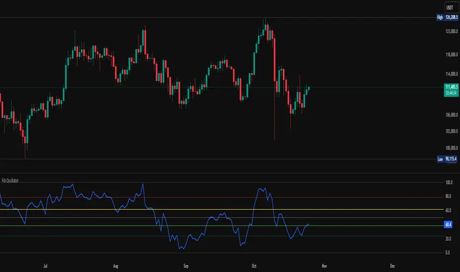
Fib OscillatorWhat is Fib Oscillator and How to Use it?
🔶 1. Conceptual Overview
The Fib Oscillator is a Fibonacci-based relative position oscillator.
Instead of measuring momentum (like RSI or MACD), it measures where price currently sits between the recent swing high and swing low, expressed as a percentage within the Fibonacci range.
In other words:
It answers: “Where is price right now within its most recent dynamic range?”
It visualizes retracement and extension zones numerically, providing continuous feedback between 0% and 100% (and beyond if extended).
🔶 2. What the Script Does
The indicator:
Automatically detects recent high and low levels using an adaptive lookback window, which depends on ATR volatility.
Calculates the current price’s position between those levels as a percentage (0–100).
Plots that percentage as an oscillator — showing visually whether price is near the top, middle, or bottom of its recent range.
Overlays Fibonacci retracement levels (23.6%, 38.2%, 50%, 61.8%, 78.6%) as reference zones.
Generates alerts when the oscillator crosses key Fib thresholds — which can signal retracement completion, breakout potential, or pullback exhaustion.
🔶 3. Technical Flow Breakdown
(a) Inputs
Input Description Default Notes
atrLength ATR period used for volatility estimation 14 Used to dynamically tune lookback sensitivity
minLookback Minimum lookback window (candles) 20 Ensures stability even in low volatility
maxLookback Maximum lookback window 100 Limits over-expansion during high volatility
isInverse Inverts chart orientation false Useful for inverse markets (e.g. shorts or inverse BTC view)
(b) Volatility-Adaptive Lookback
Instead of using a fixed lookback, it calculates:
lookback
=
SMA(ATR,10)
/
SMA(Close,10)
×
500
lookback=SMA(ATR,10)/SMA(Close,10)×500
Then it clamps this between minLookback and maxLookback.
This makes the oscillator:
More reactive during high volatility (shorter lookback)
More stable during calm markets (longer lookback)
Essentially, it self-adjusts to market rhythm — you don’t have to constantly tweak lookback manually.
(c) High-Low Reference Points
It takes the highest and lowest points within the dynamic lookback window.
If isInverse = true, it flips the candle logic (useful if viewing inverse instruments like stablecoin pairs or when analyzing bearish setups invertedly).
(d) Oscillator Core
The main oscillator line:
osc
=
(
close
−
low
)
(
high
−
low
)
×
100
osc=
(high−low)
(close−low)
×100
0% = Price is at the lookback low.
100% = Price is at the lookback high.
50% = Midpoint (balanced).
Between Fibonacci percentages (23.6%, 38.2%, 61.8%, etc.), the oscillator indicates retracement stages.
(e) Fibonacci Levels as Reference
It overlays horizontal reference lines at:
0%, 23.6%, 38.2%, 50%, 61.8%, 78.6%, 100%
These act as support/resistance bands in oscillator space.
You can read it similar to how traders use Fibonacci retracements on charts, but compressed into a single line oscillator.
(f) Alerts
The script includes built-in alert conditions for crossovers at each major Fibonacci level.
You can set TradingView alerts such as:
“Oscillator crossed above 61.8%” → possible bullish continuation or breakout.
“Oscillator crossed below 38.2%” → possible pullback or correction starting.
This allows automated monitoring of fib retracement completions without manually drawing fib levels.
🔶 4. How to Use It
🔸 Visual Interpretation
Oscillator Value Zone Market Context
0–23.6% Deep Retracement Potential exhaustion of a down-move / early reversal
23.6–38.2% Shallow retracement zone Possible continuation phase
38.2–50% Mid retracement Neutral or indecisive structure
50–61.8% Key pivot region Common trend resumption zone
61.8–78.6% Late retracement Often “last pullback” area
78.6–100% Near high range Possible overextension / profit-taking
>100% Range breakout New leg formation / expansion
🔸 Practical Application Steps
Load the indicator on your chart (set overlay = false, so it’s below the main price chart).
Observe oscillator position relative to fib bands:
Use it to determine retracement depth.
Combine with structure tools:
Trend lines, swing points, or HTF market structure.
Use crossovers for timing:
Crossing above 61.8% in an uptrend often confirms breakout continuation.
Crossing below 38.2% in a downtrend signals renewed downside momentum.
For range markets, oscillator swings between 23.6% and 78.6% can define accumulation/distribution boundaries.
🔶 5. When to Use It
During Retracements: To gauge how deep the pullback has gone.
During Range Markets: To identify relative overbought/oversold positions.
Before Breakouts: Crossovers of 61.8% or 78.6% often precede impulsive moves.
In Multi-Timeframe Contexts:
LTF (15M–1H): Detect intraday retracement exhaustion.
HTF (4H–1D): Confirm major range expansions or key reversal zones.
🔶 6. Ideal Companion Indicators
The Fib Oscillator works best when contextualized with structure, volatility, and trend bias indicators.
Below are optimal pairings:
Companion Indicator Purpose Integration Insight
Market Structure MTF Tool Identify active trend direction Use Fib Oscillator only in trend direction for cleaner signals
EMA Ribbon / Supertrend Trend confirmation Align oscillator crossovers with EMA bias
ATR Bands / Volatility Envelope Validate breakout strength If oscillator >78.6% & ATR rising → valid breakout
Volume Oscillator Confirm retracement strength Volume contraction + oscillator under 38.2% → potential reversal
HTF Fib Retracement Tool Combine LTF oscillator with HTF fib confluence Powerful multi-timeframe setups
RSI or Stochastic Measure momentum relative to position RSI divergence while oscillator near 78.6% → exhaustion clue
🔶 7. Understanding the Settings
Setting Function Practical Impact
ATR Period (14) Controls volatility sampling Higher = smoother lookback adaptation
Min Lookback (20) Smallest window allowed Lower = more reactive but noisier
Max Lookback (100) Largest window allowed Higher = smoother but slower to react
Inverse Candle Chart Flips oscillator vertically Useful when analyzing bearish or inverse scenarios (e.g. short-side fib mapping)
Recommended Configs:
For scalping/intraday: ATR 10–14, lookback 20–50
For swing/position trading: ATR 14–21, lookback 50–100
🔶 8. Example Trade Logic (Practical Use)
Scenario: Uptrend on 4H chart
Oscillator drops to below 38.2% → retracement zone
Price consolidates → oscillator stabilizes
Oscillator crosses above 50% → pullback ending
Entry: Long when oscillator crosses above 61.8%
Exit: Near 78.6–100% zone or upon divergence with RSI
For Short Bias (Inverse Setup):
Enable isInverse = true to visually flip the oscillator (so lows become highs).
Use the same thresholds inversely.
🔶 9. Strengths & Limitations
✅ Strengths
Dynamic, self-adapting to volatility
Quantifies Fib retracement as a continuous function
Compact oscillator view (no clutter on chart)
Works well across all timeframes
Compatible with both trending and ranging markets
⚠️ Limitations
Doesn’t define trend direction — must be used with structure filters
Can whipsaw during choppy consolidations
The “lookback auto-adjust” may lag in sudden volatility shifts
Shouldn’t be used standalone for entries without structural confluence
🔶 10. Summary
The “Fib Oscillator” is a dynamic Fibonacci-relative positioning tool that merges retracement theory with adaptive volatility logic.
It gives traders an intuitive, quantified view of where price sits within its recent fib range, allowing anticipation of pullbacks, reversals, or breakout momentum.
Think of it as a "Fibonacci RSI", but instead of momentum strength, it shows positional depth — the vibrational location of price within its natural swing cycle.
X rVPoCOverview
The rVPoC indicator isolates and displays the Volume Point of Control — the price level within a chosen lookback window that has accumulated the highest traded volume.
Unlike typical volume profiles that analyze an entire session or day, this version is designed for rolling intraday precision. It continually updates the VPoC using data from a lower “zoomed-in” timeframe (e.g., 1-minute) to refine accuracy, even when viewed on higher-timeframe charts.
How It Works
At its core, the indicator “zooms in” via Pine Script’s multi-timeframe engine:
Lower timeframe aggregation:
A secondary (zoomed) timeframe — by default 1-minute — is used to pull detailed OHLCV data through request.security().
Rolling window analysis:
The user-defined bars_per_current parameter determines how many of those lower-timeframe bars to include (e.g., 15 → a 15-minute rolling window).
Volume binning:
The high-to-low range of that window is divided into evenly spaced price bins (vp_price_levels). Each bin accumulates the volume of trades overlapping its range.
Point of Control selection:
The bin with the greatest accumulated volume is located, and its volume-weighted midpoint is plotted as the VPoC.
Visual output:
Discrete line-break markers are plotted for each bar, preventing the “connecting line” distortions common in continuous plots.
Use Case
This indicator is ideal for intraday traders who want to:
Track how the most active traded price shifts over time.
Identify short-term value zones forming within a 15-minute (or custom) rolling range.
Observe micro-structure behavior during developing sessions without committing to full volume profile tools.
Overlay a lightweight VPoC on top of other tools such as open-range or VWAP-based frameworks.
It is particularly effective on 1-minute and 5-minute charts, providing a granular yet efficient measure of volume concentration that updates bar-by-bar.
Summary
The VPoC indicator delivers a continuously updating micro-profile of where trading volume is most active within a chosen intraday window.
It’s designed to complement range, VWAP, and order-flow analysis by highlighting evolving value zones without visual clutter or session-anchoring logic.
Traders can interpret shifts in the VPoC as changes in short-term control — where buyers or sellers are concentrating their activity within the evolving price structure.

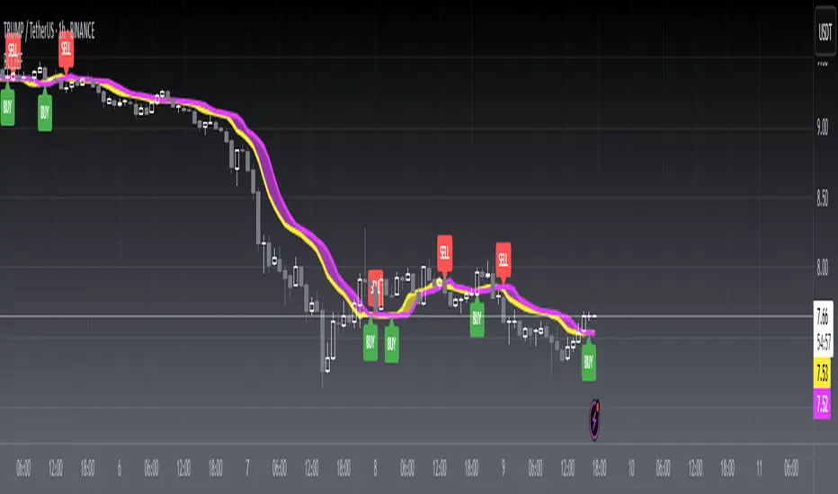
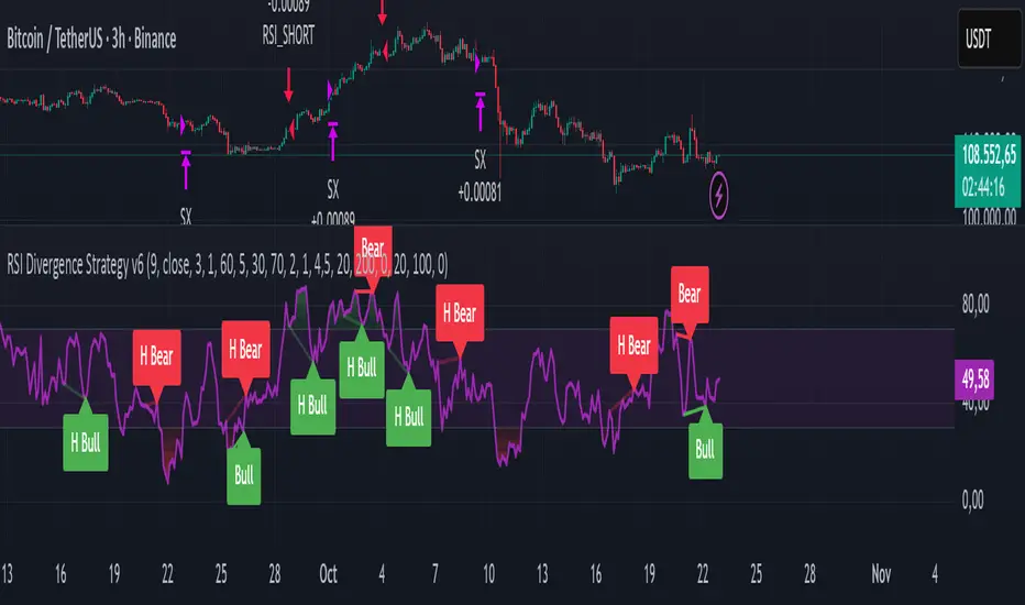
RSI Divergence Strategy v6 What this does
Detects regular and hidden divergences between price and RSI using confirmed RSI pivots. Adds RSI@pivot entry gates, a normalized strength + volume filter, optional volume gate, delayed entries, and transparent risk management with rigid SL and activatable trailing. Visuals are throttled for clarity and include a gap-free horizontal RSI gradient.
How it works (simple)
🧮 RSI is calculated on your selected source/period.
📌 RSI pivots are confirmed with left/right lookbacks (lbL/lbR). A pivot becomes final only after lbR bars; before that, it can move (expected).
🔎 The latest confirmed pivot is compared against the previous confirmed pivot within your bar window:
• Regular Bullish = price lower low + RSI higher low
• Hidden Bullish = price higher low + RSI lower low
• Regular Bearish = price higher high + RSI lower high
• Hidden Bearish = price lower high + RSI higher high
💪 Each divergence gets a strength score that multiplies price % change, RSI change, and a volume ratio (Volume SMA / Baseline Volume SMA).
• Set Min divergence strength to filter tiny/noisy signals.
• Turn on the volume gate to require volume ratio ≥ your threshold (e.g., 1.0).
🎯 RSI@pivot gating:
• Longs only if RSI at the bullish pivot ≤ 30 (default).
• Shorts only if RSI at the bearish pivot ≥ 70 (default).
⏱ Entry timing:
• Immediate: on divergence confirm (delay = 0).
• Delayed: after N bars if RSI is still valid.
• RSI-only mode: ignore divergences; use RSI thresholds only.
🛡 Risk:
• Rigid SL is placed from average entry.
• Trailing activates only after unrealized gain ≥ threshold; it re-anchors on new highs (long) or new lows (short).
What’s NEW here (vs. the reference) — and why you may care
• Improved pivots + bar window → fewer early/misaligned signals; cleaner drawings.
• RSI@pivot gates → entries aligned with true oversold/overbought at the exact decision bar.
• Normalized strength + volume gate → ignore weak or low-volume divergences.
• Delayed entries → require the signal to persist N bars if you want more confirmation.
• Rigid SL + activatable trailing → trailing engages only after a cushion, so it’s less noisy.
• Clutter control + gradient → readable chart with a smooth RSI band look.
Suggested starting values (clear ranges)
• RSI@pivot thresholds: LONG ≤ 30 (oversold), SHORT ≥ 70 (overbought).
• Min divergence strength:
0.0 = off
3–6 = moderate filter
7–12 = strict filter for noisy LTFs
• Volume gate (ratio):
1.0 = at least baseline volume
1.2–1.5 = strong-volume only (fewer but cleaner signals)
• Pivot lookbacks:
lbL 1–2, lbR 3–4 (raise lbR to confirm later and reduce noise)
• Bar window (between pivots):
Min 5–10, Max 30–60 (increase Min if you see micro-pivots; increase Max for wider structures)
• Risk:
Rigid SL 2–5% on liquid majors; 5–10% on higher-volatility symbols
Trailing activation 1–3%, trailing 0.5–1.5% are common intraday starts
Plain-text examples
• BTCUSDT 1h → RSI 9, lbL 1, lbR 3, Min strength 5.0, Volume gate 1.0, SL 4.5%, Trail on 2.0%, Trail 1.0%.
• SPY 15m → RSI 8, lbL 1, lbR 3, Min strength 7.0, Volume gate 1.2, SL 3.0%, Trail on 1.5%, Trail 0.8%.
• EURUSD 4h → RSI 14, lbL 2, lbR 4, Min strength 4.0, Volume gate 1.0, SL 2.5%, Trail on 1.0%, Trail 0.5%.
Notes & limitations
• Pivot confirmation means the newest candidate pivot can move until lbR confirms it (expected).
• Results vary by timeframe/symbol/settings; always forward-test.
• Educational tool — no performance or profit claims.
Credits
• RSI by J. Welles Wilder Jr. (1978).
• Reference divergence script by eemani123:
• This version by tagstrading 2025 adds: improved pivot engine, RSI@pivot gating, normalized strength + optional volume gate, delayed entries, rigid SL and activatable trailing, and a gap-free RSI gradient.
Experimental Supertrend [CHE]Experimental Supertrend — Combines EMA crossovers for trend regime detection with an adaptive ATR-based hull that selects the narrowest band to contain recent highs and lows, minimizing false breaks in varying volatility.
Summary
This indicator overlays a dynamic supertrend boundary around a midline derived from dual EMAs, using EMA crossovers to switch between bullish and bearish regimes. The hull adapts by evaluating multiple ATR periods and selecting the tightest one that fully encloses price action over a specified window, which helps in creating more stable trend lines that hug price without excessive gaps or breaches. Fills between the midline and hull provide visual cues for trend strength, darkening temporarily after regime changes to highlight transitions. Alerts trigger on crossovers, and markers label entry points, making it suitable for trend-following setups where standard supertrends might whipsaw. Overall, it offers robustness through auto-adjustment, reducing sensitivity to noise while maintaining responsiveness to genuine shifts.
Motivation: Why this design?
Standard supertrend indicators often flip prematurely in choppy markets due to fixed multipliers that do not account for localized volatility patterns, leading to frequent false signals and eroded confidence in trends. This design addresses that by incorporating an EMA-based regime filter for directional bias and an auto-adaptive hull that dynamically tunes the band width based on recent price containment needs. By prioritizing the narrowest effective enclosure, it avoids over-wide bands in calm periods that cause lag or under-wide ones in volatility spikes that invite breaks, providing a more consistent trailing reference without manual tweaking.
What’s different vs. standard approaches?
- Reference baseline: Diverges from the classic ATR-multiplier supertrend, which uses a single fixed period and constant factor applied to close or high/low deviations.
- Architecture differences:
- Auto-selection from candidate ATR lengths to find the optimal period for current conditions.
- Dynamic multiplier clamped between floor and cap values, adjusted by padding to ensure reliable containment.
- Regime-gated rendering, where hull position flips based on EMA relative positioning.
- Post-transition visual fading to emphasize change points without altering core logic.
- Practical effect: Charts show tighter, more reactive bands that rarely breach during trends, reducing visual clutter from flips; the adaptive nature means less intervention across assets, as the hull self-adjusts to volatility clusters rather than applying a one-size-fits-all scale.
How it works (technical)
The indicator first computes two EMAs from close prices using lengths derived from a preset pair or manual inputs, establishing a midline as their average. This midline serves as the central reference for the hull. True range values are then smoothed into multiple ATR candidates using exponential weighting over the specified lengths. For each candidate, deviations of recent highs and lows from the midline are ratioed against the ATR to determine a required multiplier that would enclose all extremes in the containment window—the highest ratio plus padding sets the base, clamped to user-defined bounds. Among valid candidates (those with sufficient history), the one yielding the narrowest overall band width is selected. The hull boundaries are then offset from the midline by this multiplier times the chosen ATR, and further smoothed with a fixed EMA to reduce jitter. Regime direction from EMA comparison gates which boundary acts as support or resistance, with initialization seeding arrays on the first bar to handle state persistence. No higher timeframe data is used, so all logic runs on the chart's native bars without lookahead.
Parameter Guide
EMA Pair — Selects preset lengths for fast and slow EMAs, influencing regime sensitivity and midline stability. Default: "21/55". Trade-offs/Tips: Faster pairs like "9/21" increase cross frequency for scalping but raise false signals; slower like "50/200" smooths for swings, potentially missing early turns. Use Manual for fine control.
Manual Fast — Sets fast EMA length when Manual mode is active; shorter values make regime switches quicker. Default: 21. Trade-offs/Tips: Lower than 10 risks over-reactivity; pair with slow at least double for clear separation.
Manual Slow — Sets slow EMA length when Manual mode is active; longer values anchor the midline more firmly. Default: 55. Trade-offs/Tips: Above 100 adds lag in trends; balance with fast to avoid perpetual neutrality.
ATR Lengths (comma-separated) — Defines candidate periods for ATR smoothing; more options allow finer auto-selection. Default: "7,10,14,21,28,35". Trade-offs/Tips: Fewer candidates speed computation but may miss optimal fits; keep under 10 for efficiency.
Containment Window — Number of recent bars the hull must fully enclose highs/lows of; larger windows favor stability. Default: 50. Trade-offs/Tips: Shorter (under 20) adapts faster to breaks but increases breach risk; longer smooths but delays response.
Min Multiplier Floor — Lowest allowed multiplier for hull width; prevents overly tight bands in low volatility. Default: 0.5. Trade-offs/Tips: Raise to 0.75 for conservative enclosures; too low allows pinches that flip easily.
Max Multiplier Cap — Highest allowed multiplier; caps expansion in spikes to avoid wide, lagging bands. Default: 1.0. Trade-offs/Tips: Lower to 0.75 tightens overall; higher permits more room but risks detachment from price.
Padding (+) — Adds buffer to the auto-multiplier for safer containment without exact touches. Default: 0.05. Trade-offs/Tips: Increase to 0.10 in gappy markets; minimal values hug closer but may still breach on outliers.
Fill Between (Mid ↔ Supertrend) — Toggles shaded area between midline and active hull for trend visualization. Default: true. Trade-offs/Tips: Disable for cleaner charts; pairs well with transparency tweaks.
Base Fill Transparency (0..100) — Sets default opacity of fills; higher values make them subtler. Default: 80. Trade-offs/Tips: Under 50 overwhelms price action; adjust with darken boost for emphasis.
Darken on Trend Change — Enables temporary opacity increase after regime shifts to spotlight transitions. Default: true. Trade-offs/Tips: Off for steady visuals; on aids spotting reversals in real-time.
Darken Fade Bars — Duration in bars for the darken effect to ramp back to base; longer prolongs highlight. Default: 8. Trade-offs/Tips: Shorter (4-6) for fast-paced charts; longer holds attention on changes.
Darken Boost at Change (Δ transp) — Intensity of opacity reduction at crossover; higher values make shifts more prominent. Default: 50. Trade-offs/Tips: Cap at 70 to avoid blackout; tune down if fades obscure details.
Show Supertrend Line — Displays the active hull boundary as a line. Default: true. Trade-offs/Tips: Hide for fill-only views; linewidth fixed at 3 for visibility.
Show EMA Cross Markers — Places circles and labels at crossover points for entry cues. Default: true. Trade-offs/Tips: Disable in clutter; labels show "Buy"/"Sell" at absolute positions.
Alert: EMA Cross Up (Long) — Triggers notification on bullish crossover. Default: true. Trade-offs/Tips: Pair with filters; once-per-bar frequency.
Alert: EMA Cross Down (Short) — Triggers notification on bearish crossover. Default: true. Trade-offs/Tips: Use for exits; ensure broker integration.
Show Debug — Reveals internal diagnostics like selected ATR details (if implemented). Default: false. Trade-offs/Tips: Enable for troubleshooting selections; minimal overhead.
Reading & Interpretation
Bullish regime shows a green line below price as support, with upward fill from midline; bearish uses red line above as resistance, downward fill. Crossovers flip the active boundary, marked by tiny green/red circles and "Buy"/"Sell" labels at the hull level. Fills start at base transparency but darken sharply at changes, fading over the specified bars to signal fresh momentum. If the hull rarely breaches during trends, containment is effective; frequent touches without flips indicate tight adaptation. Debug mode (when enabled) overlays text or plots for selected length and multiplier, helping verify auto-choices.
Practical Workflows & Combinations
- Trend following: Enter long on green "Buy" label above prior low structure; confirm with higher high. Trail stops along the green hull line, tightening as fills stabilize post-fade.
- Exits/Stops: Conservative exit on opposite crossover or hull breach; aggressive hold until fade completes if volume supports. Use darken boost as a volatility cue—high delta suggests waiting for confirmation.
- Multi-asset/Multi-TF: Defaults suit forex/stocks on 15m-4h; for crypto, widen containment to 75 for gaps. Layer on volume oscillator for cross filters; avoid on low-liquidity assets where ATR candidates skew.
Behavior, Constraints & Performance
Closed-bar logic ensures signals confirm at bar end, with live bars updating hull adaptively but no repaints since no future data or security calls are used. Arrays persist ATR states across bars, initialized once with candidates parsed from string. Small fixed loops (over 6 lengths max, inner up to 50) run per bar, capped by max_bars_back=500 for history needs. Resources stay low with 500 labels/lines limits, but dense charts may hit on markers. Known limits include initial lag until containment history builds (50+ bars), potential wide bands on gaps, and suboptimal selections if candidates omit ideal lengths.
Sensible Defaults & Quick Tuning
Start with "21/55" pair, 50-window, 0.5-1.0 multipliers, and 80% transparency for balanced responsiveness on daily charts. For too many flips, raise min floor to 0.75 or add lengths like "42"; for sluggishness, shorten window to 30 or pick faster pair. In high-vol environments, boost padding to 0.10; for smoother visuals, extend fade bars to 12.
What this indicator is—and isn’t
This is a visualization and signal layer for trend regime and adaptive boundaries, aiding entry/exit timing in directional markets. It is not a standalone system—pair with price structure, risk sizing, and broader context. Not predictive of turns, just reactive to containment and crosses.
Disclaimer
The content provided, including all code and materials, is strictly for educational and informational purposes only. It is not intended as, and should not be interpreted as, financial advice, a recommendation to buy or sell any financial instrument, or an offer of any financial product or service. All strategies, tools, and examples discussed are provided for illustrative purposes to demonstrate coding techniques and the functionality of Pine Script within a trading context.
Any results from strategies or tools provided are hypothetical, and past performance is not indicative of future results. Trading and investing involve high risk, including the potential loss of principal, and may not be suitable for all individuals. Before making any trading decisions, please consult with a qualified financial professional to understand the risks involved.
By using this script, you acknowledge and agree that any trading decisions are made solely at your discretion and risk.
Do not use this indicator on Heikin-Ashi, Renko, Kagi, Point-and-Figure, or Range charts, as these chart types can produce unrealistic results for signal markers and alerts.
Happy trading
Chervolino

Herd Flow Oscillator — Volume Distribution Herd Flow Oscillator — Scientific Volume Distribution (herd-accurate rev)
A composite order-flow oscillator designed to surface true herding behavior — not just random bursts of buying or selling.
It’s built to detect when market participants start acting together, showing persistent, one-sided activity that statistically breaks away from normal market randomness.
Unlike traditional volume or momentum indicators, this tool doesn’t just look for “who’s buying” or “who’s selling.”
It tries to quantify crowd behavior by blending multiple statistical tests that describe how collective sentiment and coordination unfold in price and volume dynamics.
What it shows
The Herd Flow Oscillator works as a multi-layer detector of crowd-driven flow in the market. It examines how signed volume (buy vs. sell pressure) evolves, how persistent it is, and whether those actions are unusually coordinated compared to random expectations.
HerdFlow Composite (z) — the main signal line, showing how statistically extreme the current herding pressure is.
When this crosses above or below your set thresholds, it suggests a high probability of collective buying or selling.
You can optionally reveal component panels for deeper insight into why herding is detected:
DVI (Directional Volume Imbalance): Measures the ratio of bullish vs. bearish volume.
If it’s strongly positive, more volume is hitting the ask (buying); if negative, more is hitting the bid (selling).
LSV-style Herd Index : Inspired by academic finance measures of “herding.”
It compares how often volume is buying vs. selling versus what would happen by random chance.
If the result is significantly above chance, it means traders are collectively biased in one direction.
O rder-Flow Persistence (ρ 1..K): Averages autocorrelation of signed volume over several lags.
In simpler terms: checks if buying/selling pressure tends to continue in the same direction across bars.
Positive persistence = ongoing coordination, not just isolated trades.
Runs-Test Herding (−Z) : Statistical test that checks how often trade direction flips.
When there are fewer direction changes than expected, it means trades are clustering — a hallmark of herd behavior.
Skew (signed volume): Measures whether signed volume is heavily tilted to one side.
A positive skew means more aggressive buying bursts; a negative skew means more intense selling bursts.
CVD Slope (z): Looks at the slope of the Cumulative Volume Delta — essentially how quickly buy/sell pressure is accelerating.
It’s a short-term flow acceleration measure.
Shapes & background
▲ “BH” at the bottom = Bull Herding; ▼ “BH-” at the top = Bear Herding.
These markers appear when all conditions align to confirm a herding regime.
Persistence and clustering both confirm coordinated downside flow.
Core Windows
Primary Window (N) — the main sample length for herding calculations.
It’s like the "memory span" for detecting coordinated behavior. A longer N means smoother, more reliable signals.
Short Window (Nshort) — used for short-term measurements like imbalance and slope.
Smaller values react faster but can be noisy; larger values are steadier but slower.
Long Window (Nlong) — used for z-score normalization (statistical scaling).
This helps the indicator understand what’s “normal” behavior over a longer horizon, so it can spot when things deviate too far.
Autocorr lags (acLags) — how many steps to check when measuring persistence.
Higher values (e.g., 3–5) look further back to see if trends are truly continuing.
Calculation Options
Price Proxy for Tick Rule — defines how to decide if a trade is “buy” or “sell.”
hlc3 (average of high, low, and close) works as a neutral, smooth price proxy.
Use ATR for scaling — keeps signals comparable across assets and timeframes by dividing by volatility (ATR).
Prevents high-volatility periods from dominating the signal.
Median Filter (bars) — smooths out erratic data spikes without heavily lagging the response.
Odd values like 3 or 5 work best.
Signal Thresholds
Composite z-threshold — determines how extreme behavior must be before it counts as “herding.”
Higher values = fewer, more confident signals.
Imbalance threshold — the minimum directional volume imbalance to trigger interest.
Plotting
Show component panels — useful for analysts and developers who want to inspect the math behind signals.
Fill strong herding zones — purely visual aid to highlight key periods of coordinated trading.
How to use it (practical tips)
Understand the purpose: This is not just a “buy/sell” tool.
It’s a behavioral detector that identifies when traders or algorithms start acting in the same direction.
Timeframe flexibility:
15m–1h: reveals short-term crowd shifts.
4h–1D: better for swing-trade context and institutional positioning.
Combine with structure or trend:
When HerdFlow confirms a bullish regime during a breakout or retest, it adds confidence.
Conversely, a bearish cluster at resistance may hint at a crowd-driven rejection.
Threshold tuning:
To make it more selective, increase zThr and imbThr.
To make it more sensitive, lower those thresholds but expand your primary window N for smoother results.
Cross-market consistency:
Keep “Use ATR for scaling” enabled to maintain consistency across different instruments or timeframes.
Denoising:
A small median filter (3–5 bars) removes flicker from volume spikes but still preserves the essential crowd patterns.
Reading the components (why signals fire)
Each sub-metric describes a unique “dimension” of crowd behavior:
DVI: how imbalanced buying vs selling is.
Herd Index: how biased that imbalance is compared to random expectation.
Persistence (ρ): how continuous those flows are.
Runs-Test: how clumped together trades are — clustering means the crowd’s acting in sync.
Skew: how lopsided the volume distribution is — sudden surges of one-sided aggression.
CVD Slope: how strongly accelerating the current directional flow is.
When all of these line up, you’re seeing evidence that market participants are collectively moving in the same direction — i.e., true herding.
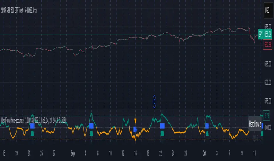
ATR Regime Filter (median & P70)ATR Regime Filter (Median & P70)
Purpose
Filter your signals by the volatility regime. The indicator compares the current ATR to two rolling statistical thresholds—the median (P50) and the 70th percentile (P70)—to avoid trading during quiet phases and prioritize setups when the market “breathes.”
How it works
Computes ATR(14) on a user-defined source timeframe (srcTF) via request.security.
Converts a target window in days (days) into bars of the source TF.
Due to Pine limits, the effective window is capped at 5000 bars (shown in an optional label).
Calculates Median (P50) and P70 of ATR over the effective window.
Exposes two booleans:
ATR > Median (normal-to-elevated volatility)
ATR > P70 (elevated volatility)
Display
Plots: ATR, Median, P70.
Panel background (bgcolor):
light green when ATR > P70
teal when ATR > Median
neutral otherwise
Optional label: shows source TF, effective window size (bars & days), and the boolean states.
Inputs
ATR length (default 14)
TF source ATR (srcTF, e.g., “1”, “5”, “15”)
Target window (days) (days, default 20)
Show label (bool)
Suggested use
Breakout/Momentum: require ATR > P70 in addition to your breakout conditions (close beyond level, volume, retest).
Range/Mean reversion: at minimum require ATR > Median.
In strategies, use ATR > Median/P70 as a filter alongside price structure, volume, and EMAs.
Limitations
On very short source TFs (e.g., 1-min), the window may be clipped to 5000 bars (~3.5 days). Increase srcTF (5m/15m) if you want a true 15–30 day history.
ATR measures magnitude, not direction—combine with trend/structure signals.

TwinPulse Q Lead SPY x QQQ Intermarket Pulse 1HTwinPulse Q Lead is a concise one hour indicator for SPY and QQQ that converts three sources of market information into a single pulse line, a mode readout with BUY SELL WAIT, and compact alerts. It blends intermarket leadership between QQQ and SPY, intraday flow from the slope of session VWAP, and where the current price sits inside the regular trading hours range. The three components are normalized, fused, compressed to a stable range, and smoothed for clear thresholds. The aim is a readable intraday regime signal that helps you decide when to participate and when to stand aside.
The script is built with Pine v6, uses request security with lookahead off, and does not repaint. It is an indicator, not a strategy. It does not contain any solicitation, links, or outside references. The description is self contained and explains both logic and use so that any trader can understand the design without reading code.
What makes this original and useful
Intermarket leadership is measured directly from QQQ and SPY on your working timeframe using a Z score of the return spread. When growth is leading value heavy large caps, leadership turns positive. When it lags, leadership turns negative. This gives a real time read of the Nasdaq versus S and P tug of war that most day traders watch informally.
Intraday flow is taken from the slope of the session VWAP. A linear regression of VWAP over a short window captures whether value is rising or falling inside the day. Dividing by ATR normalizes slope by typical movement so that the signal is comparable across weeks.
Session position places price inside the current regular hours high to low. It answers whether the day is trading in the top half, the bottom half, or the middle. This is a simple but powerful context filter for breakouts and fades.
The three components are fused into one pulse, compressed with either hyperbolic tangent or softsign to keep values bounded, and then smoothed by a short EMA. This yields a stable range with a zero line so the eye can read shifts quickly.
The panel shows a human readable mode with reasons and a strength score. Traders who do not want to read lines can rely on a simple state and a compact justification that explains why the state is set.
This is not a mashup that simply overlays unrelated indicators. Each component was chosen to answer a distinct question that is common to SPY and QQQ intraday decision making. Leadership answers who is in charge, flow answers whether value inside the session is building or leaking, and position answers if price is pressing the extremes or circling the middle. The pulse ties the three together and prevents any single component from dominating.
How the calculations work
Leadership. Compute a short rate of change for SPY and QQQ. Subtract SPY from QQQ to get spread returns, then compute a rolling Z score over a longer window. Positive values mean QQQ is leading. Negative values mean SPY is leading.
Flow. Compute session VWAP on the active symbol. Regress VWAP over a short window to obtain a slope estimate. Divide by ATR to scale slope by current volatility so that a small rise on a quiet day is not treated the same as a small rise on a wild day.
Position. Track the highest high and lowest low since the start of regular hours. Place the current close inside that range on a zero to one scale, then recenter to a minus one to plus one scale. Positive means the top half of the day, negative means the bottom half.
Fusion. Multiply each component by a weight so users can emphasize or de emphasize leadership, flow, or position. Sum to a raw pulse.
Compression. Pass the raw pulse through a bounded function. Hyperbolic tangent is smooth and has natural saturation near the extremes. Softsign is faster and behaves like a smoother version of sign near zero. Compression avoids unbounded excursions and makes thresholds meaningful across days.
Smoothing. Apply a short EMA to the compressed pulse to reduce noise. This creates the main line called TwinPulse in the plot.
Thresholds. You can use static symmetric levels or adaptive levels. The adaptive option computes a mean and a standard deviation of the smoothed pulse over a user window, then sets upper and lower thresholds as mean plus or minus sigma times standard deviation. This allows thresholds to adjust across regimes. Static levels are still available for traders who want repeatable levels.
Events and mode. A long event fires when the smoothed pulse crosses the upper threshold with positive flow and any optional filters agree. A short event fires on the symmetric condition. The mode reads the current state rather than fire and forget. It returns BUY when the smoothed pulse is above the upper threshold with positive flow, SELL when the smoothed pulse is below the lower threshold with negative flow, otherwise WAIT. A cooldown controls how often events can fire so alerts do not spam during choppy periods.
Inputs and default values
The script ships with defaults chosen for SPY and QQQ on one hour charts.
Symbols. SPY and QQQ by default. You can switch to any pair. Many users may test IWM versus SPY for small cap reads.
Regular hours selector. On by default. This restricts the position factor to New York regular hours. Turn it off if you prefer full session behavior.
ROC length is three bars. Z score length is fifty bars. VWAP slope window is ten bars. ATR length is fourteen bars. Pulse smoothing length is three bars.
Compression mode. Choose hyperbolic tangent or softsign. Hyperbolic tangent is default.
Weights. Leadership and flow are one by default. Position is set to zero point seven to give a modest influence to where price sits inside the day.
Thresholds. Adaptive thresholds are on by default with a lookback of one hundred bars and a sigma width of zero point eight. Static levels at plus or minus zero point six are ready if you disable adaptive mode.
Filters. ADX filter is off by default. If you enable it, the script requires ADX above a user minimum before it will signal. Higher time frame confirmation is off by default. When enabled it compares the smoothed pulse on the confirm timeframe to zero and requires alignment for longs or shorts.
Cooldown. Three bars by default so that alerts do not trigger too frequently.
UI. Bar coloring is on by default. The panel is on by default and sits at the top right.
All request security calls use lookahead off and will not request future data. All persistent state variables are assigned in a way that prevents repainting. The indicator does not use non standard chart types in its logic.
How to use the indicator
Load a one hour chart of SPY or QQQ. Keep a clean chart so that the script output is easy to read.
Turn on regular hours if you want the session position to reflect the cash session. This is recommended for SPY and QQQ.
Watch the panel. Mode reads BUY or SELL or WAIT. The strength value is a simple vote based score that ranges from zero to one hundred. It counts leadership, flow, ADX if enabled, and higher time frame confirmation if enabled. You can use strength to filter weak states.
Consider action only when mode is BUY or SELL and the signal has not just fired on the last bar. The triangles mark where an event fired. Alerts use the same logic as the events. WAIT means stand aside.
To slow the system, enable ADX and set a higher minimum or enable higher time frame confirmation. To speed it up, disable the filters, disable adaptive thresholds, or tighten the sigma width.
When publishing, use a clean chart with only this indicator. Show the symbol and timeframe clearly and make sure the plot legend is visible. If you add drawings on the chart, only include ones that help readers understand the output.
Publication notes and compliance
This description is written in English. The title uses ASCII and only uses capital letters for common abbreviations. The script is original and explains how and why the components work together. There are no links or promotional material. The script does not claim performance. It does not use lookahead. The panel and alerts exist to help a human read and act with discipline. The indicator can be published as open source or as protected. If you choose protected, the description still allows readers to understand how the logic works without access to the code.
If you later convert the logic into a strategy for publication, use realistic commission and slippage, risk no more than a small share of equity per trade, and choose a dataset that yields a large enough sample. Explain any deviations from these default recommendations in your strategy description. Do not publish results from non standard chart types since they can mislead readers on signal timing.
Limitations and risks
Intermarket leadership is a relative measure. There are hours when both SPY and QQQ fall while leadership remains positive. Treat leadership as a context, not a stand alone trigger.
VWAP slope is a path measure inside the session. It can flip several times on a choppy day. That is why the script uses a short smoothing and an optional cooldown. Use ADX or higher time frame confirmation to avoid the worst chop.
Session position assumes a meaningful regular hours range. On half days or around openings with gaps the position factor can be less informative. If this bothers you, reduce the weight of position or turn it off.
Compression and smoothing introduce lag by design. The goal is stability and clarity. If you want earlier but noisier signals, reduce smoothing and weights, and use static thresholds.
No indicator guarantees future results. TwinPulse Q Lead is a decision aid. It should be combined with your risk rules, position size policy, and a clear exit plan. Past behavior is not a promise for the future.
Frequently asked questions
What symbols are supported. Any symbol can be used as the chart symbol. Leadership uses the two user symbols which default to SPY and QQQ. Many traders may try IWM versus SPY or DIA versus SPY.
Can I change the timeframe. Yes, but the design target is one hour. On very short timeframes the VWAP slope becomes very sensitive and you should consider stronger filters.
Does the script repaint. No. It uses request security with lookahead off and the panel updates on the last bar only. Events are based on bar close conditions unless you attach alerts on any alert function call which will still respect the logic without looking into the future.
How are the strength numbers built. The strength score is the share of aligned votes across leadership, flow, ADX if enabled, and higher time frame confirmation if enabled. A value near one hundred means many filters agree. A value near fifty means partial alignment. It is not a probability or an accuracy number.
Can I use non standard chart types. You can view the indicator on them but do not publish signals from non standard chart types because that can mislead readers about timing. Use classic candles or bars when you publish and when you test.
Why do I sometimes see BUY but the price is not moving. A BUY mode requires pulse above the upper threshold and positive flow. It does not require higher highs immediately. Treat BUY as a permission to look for entries using your own execution rules.

Aggregated Scores Oscillator [Alpha Extract]A sophisticated risk-adjusted performance measurement system that combines Omega Ratio and Sortino Ratio methodologies to create a comprehensive market assessment oscillator. Utilizing advanced statistical band calculations with expanding and rolling window analysis, this indicator delivers institutional-grade overbought/oversold detection based on risk-adjusted returns rather than traditional price movements. The system's dual-ratio aggregation approach provides superior signal accuracy by incorporating both upside potential and downside risk metrics with dynamic threshold adaptation for varying market conditions.
🔶 Advanced Statistical Framework
Implements dual statistical methodologies using expanding and rolling window calculations to create adaptive threshold bands that evolve with market conditions. The system calculates cumulative statistics alongside rolling averages to provide both historical context and current market regime sensitivity with configurable window parameters for optimal performance across timeframes.
🔶 Dual Ratio Integration System
Combines Omega Ratio analysis measuring excess returns versus deficit returns with Sortino Ratio calculations focusing on downside deviation for comprehensive risk-adjusted performance assessment. The system applies configurable smoothing to both ratios before aggregation, ensuring stable signal generation while maintaining sensitivity to regime changes.
// Omega Ratio Calculation
Excess_Return = sum((Daily_Return > Target_Return ? Daily_Return - Target_Return : 0), Period)
Deficit_Return = sum((Daily_Return < Target_Return ? Target_Return - Daily_Return : 0), Period)
Omega_Ratio = Deficit_Return ≠ 0 ? (Excess_Return / Deficit_Return) : na
// Sortino Ratio Framework
Downside_Deviation = sqrt(sum((Daily_Return < Target_Return ? (Daily_Return - Target_Return)² : 0), Period) / Period)
Sortino_Ratio = (Mean_Return / Downside_Deviation) * sqrt(Annualization_Factor)
// Aggregated Score
Aggregated_Score = SMA(Omega_Ratio, Omega_SMA) + SMA(Sortino_Ratio, Sortino_SMA)
🔶 Dynamic Band Calculation Engine
Features sophisticated threshold determination using both expanding historical statistics and rolling window analysis to create adaptive overbought/oversold levels. The system incorporates configurable multipliers and sensitivity adjustments to optimize signal timing across varying market volatility conditions with automatic band convergence logic.
🔶 Signal Generation Framework
Generates overbought conditions when aggregated score exceeds adjusted upper threshold and oversold conditions below lower threshold, with neutral zone identification for range-bound markets. The system provides clear binary signal states with background zone highlighting and dynamic oscillator coloring for intuitive market condition assessment.
🔶 Enhanced Visual Architecture
Provides modern dark theme visualization with neon color scheme, dynamic oscillator line coloring based on signal states, and gradient band fills for comprehensive market condition visualization. The system includes zero-line reference, statistical band plots, and background zone highlighting with configurable transparency levels.
snapshot
🔶 Risk-Adjusted Performance Analysis
Utilizes target return parameters for customizable risk assessment baselines, enabling traders to evaluate performance relative to specific return objectives. The system's focus on downside deviation through Sortino analysis provides superior risk-adjusted signals compared to traditional volatility-based oscillators that treat upside and downside movements equally.
🔶 Multi-Timeframe Adaptability
Features configurable calculation periods and rolling windows to optimize performance across various timeframes from intraday to long-term analysis. The system's statistical foundation ensures consistent signal quality regardless of timeframe selection while maintaining sensitivity to market regime changes through adaptive band calculations.
🔶 Performance Optimization Framework
Implements efficient statistical calculations with optimized variable management and configurable smoothing parameters to balance responsiveness with signal stability. The system includes automatic band adjustment mechanisms and rolling window management for consistent performance across extended analysis periods.
This indicator delivers sophisticated risk-adjusted market analysis by combining proven statistical ratios in a unified oscillator framework. Unlike traditional overbought/oversold indicators that rely solely on price movements, the ASO incorporates risk-adjusted performance metrics to identify genuine market extremes based on return quality rather than price volatility alone. The system's adaptive statistical bands and dual-ratio methodology provide institutional-grade signal accuracy suitable for systematic trading approaches across cryptocurrency, forex, and equity markets with comprehensive visual feedback and configurable risk parameters for optimal strategy integration.

MultiSessions traderglobal.topEste indicador de sesiones está diseñado para traders intradía que desean visualizar con precisión la actividad y la volatilidad característica de cada mercado. Basado en Pine Script v5 y optimizado para la zona horaria “America/New_York”, divide el día en sub-sesiones configurables y resalta sus rangos de precio en tiempo real. En particular, incorpora tres bloques para New York (NY1, NY2, NY3), dos para Londres (LON1, LON2), dos para Tokio (TKO1, TKO2) y mantiene Sídney como sesión opcional. Cada bloque puede activarse o desactivarse de forma independiente y cuenta con su propio color ajustable, lo que permite construir mapas visuales claros para estrategias basadas en horario, solapamientos y micro-estructuras de mercado.
El panel de inputs incluye la opción “Activate High/Low View”. Cuando está activada, el indicador calcula de manera incremental el mínimo y máximo de cada sub-sesión y sombrea el área entre ambos con fill, proporcionando una referencia inmediata del rango intrasesión (útil para medir compresión/expansión y posibles rompimientos). Cuando está desactivada, emplea un simple bgcolor por bloque, ideal para traders que prefieren un gráfico más limpio y solo desean distinguir visualmente los tramos horarios.
La lógica central utiliza dos funciones auxiliares: is_session(sess), que detecta si la vela actual pertenece a un tramo horario concreto, e is_newbar(sess), que determina el inicio de una nueva barra de referencia según la resolución elegida (D, W o M). Gracias a esta combinación, en cada sub-sesión el indicador reinicia sus contadores de alto y bajo al comenzar el período y los actualiza vela a vela mientras el bloque siga activo. Este enfoque evita mezclas de datos entre sesiones y asegura que el rango que se muestra corresponda estrictamente al segmento horario configurado.
Los horarios por defecto están pensados para Forex y contemplan casos que cruzan medianoche (por ejemplo, Tokio 2 y Sídney). Pine Script admite rangos como 2200-0200; no obstante, si tu bróker o la zona horaria del gráfico generan un sombreado parcial, basta con dividir el tramo en dos: 2200-2359 y 0000-0200. Asimismo, cada input.session incluye el patrón :1234567 para habilitar los siete días; puedes restringir días según tu operativa.
En cuanto al uso práctico, el indicador facilita identificar: (1) la estructura del rango por sub-sesión (útil para estrategias de breakout/mean-reversion), (2) los solapamientos entre Londres y New York, donde suele concentrarse la liquidez, y (3) períodos de menor volatilidad (tramos tardíos de Asia o previos a noticias). El color independiente por bloque te permite codificar visualmente la importancia o tu plan de trading (por ejemplo, tonos más intensos en ventanas de alta probabilidad).
Finalmente, su diseño modular hace sencilla la personalización: puedes ajustar colores, activar/desactivar bloques, cambiar horarios y modificar la resolución de reseteo del rango. Como posible mejora, se pueden añadir alertas de ruptura de máximos/mínimos de sub-sesión o etiquetas con la altura del rango (pips) al cierre. Este indicador no sustituye el juicio del trader ni constituye recomendación financiera, pero ofrece una base visual robusta para integrar el factor tiempo en la toma de decisiones.
This sessions indicator is built for intraday traders who want a precise, time-aware view of market activity and typical volatility patterns across the day. Written in Pine Script v5 and optimized for the “America/New_York” timezone, it divides the trading day into configurable sub-sessions and highlights their price ranges in real time. Specifically, it provides three blocks for New York (NY1, NY2, NY3), two for London (LON1, LON2), two for Tokyo (TKO1, TKO2), and keeps Sydney as an optional session. Each block can be enabled or disabled independently and comes with its own adjustable color, letting you build clear visual maps for time-based strategies, overlaps, and microstructure nuances.
In the inputs panel you’ll find the “Activate High/Low View” option. When enabled, the indicator incrementally computes each sub-session’s low and high and shades the area between them with fill, giving you an immediate reference to the intra-session range (useful for gauging compression/expansion and potential breakouts). When disabled, it switches to a clean bgcolor background by block—ideal if you prefer a minimal chart and simply want to distinguish time windows at a glance.
The core logic relies on two helper functions: is_session(sess), which detects whether the current bar falls within a given time window, and is_newbar(sess), which identifies the start of a new reference bar according to your chosen reset resolution (D, W, or M). With this combination, each sub-session resets its high/low at the beginning of the period and updates them bar by bar while the block remains active. This prevents cross-contamination between sessions and ensures the range you see belongs strictly to the configured segment.
Default hours are suited to Forex and include segments that cross midnight (e.g., Tokyo 2 and Sydney). Pine Script supports ranges like 2200-0200; however, if your broker or chart timezone causes partial shading, simply split the segment into two: 2200-2359 and 0000-0200. Each input.session uses the :1234567 suffix to enable all seven days; you can easily restrict days to match your plan.
Practically speaking, the indicator helps you identify: (1) range structure by sub-session (great for breakout or mean-reversion frameworks), (2) overlaps between London and New York, where liquidity and directional moves often concentrate, and (3) lower-volatility windows (late Asia or pre-news lulls). Independent colors per block let you visually encode priority or your trading plan (for example, richer tones in high-probability windows).
Thanks to its modular design, customization is straightforward: adjust colors, toggle blocks, change hours, and tweak the range-reset resolution to suit your routine. As a natural extension, you can add alerts for sub-session high/low breakouts or labels that display the range height (in pips) at session close. While no indicator replaces trader judgment or constitutes financial advice, this tool offers a robust visual foundation for incorporating the time factor directly into your decision-making, helping you contextualize price action within the rhythm of global trading sessions.
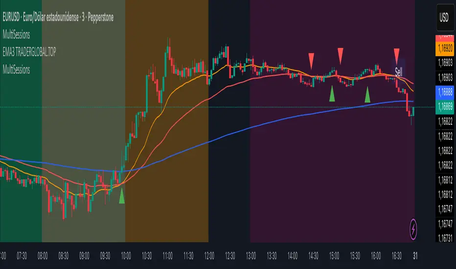
MERV: Market Entropy & Rhythm Visualizer [BullByte]The MERV (Market Entropy & Rhythm Visualizer) indicator analyzes market conditions by measuring entropy (randomness vs. trend), tradeability (volatility/momentum), and cyclical rhythm. It provides traders with an easy-to-read dashboard and oscillator to understand when markets are structured or choppy, and when trading conditions are optimal.
Purpose of the Indicator
MERV’s goal is to help traders identify different market regimes. It quantifies how structured or random recent price action is (entropy), how strong and volatile the movement is (tradeability), and whether a repeating cycle exists. By visualizing these together, MERV highlights trending vs. choppy environments and flags when conditions are favorable for entering trades. For example, a low entropy value means prices are following a clear trend line, whereas high entropy indicates a lot of noise or sideways action. The indicator’s combination of measures is original: it fuses statistical trend-fit (entropy), volatility trends (ATR and slope), and cycle analysis to give a comprehensive view of market behavior.
Why a Trader Should Use It
Traders often need to know when a market trend is reliable vs. when it is just noise. MERV helps in several ways: it shows when the market has a strong direction (low entropy, high tradeability) and when it’s ranging (high entropy). This can prevent entering trend-following strategies during choppy periods, or help catch breakouts early. The “Optimal Regime” marker (a star) highlights moments when entropy is very low and tradeability is very high, typically the best conditions for trend trades. By using MERV, a trader gains an empirical “go/no-go” signal based on price history, rather than guessing from price alone. It’s also adaptable: you can apply it to stocks, forex, crypto, etc., on any timeframe. For example, during a bullish phase of a stock, MERV will turn green (Trending Mode) and often show a star, signaling good follow-through. If the market later grinds sideways, MERV will shift to magenta (Choppy Mode), warning you that trend-following is now risky.
Why These Components Were Chosen
Market Entropy (via R²) : This measures how well recent prices fit a straight line. We compute a linear regression on the last len_entropy bars and calculate R². Entropy = 1 - R², so entropy is low when prices follow a trend (R² near 1) and high when price action is erratic (R² near 0). This single number captures trend strength vs noise.
Tradeability (ATR + Slope) : We combine two familiar measures: the Average True Range (ATR) (normalized by price) and the absolute slope of the regression line (scaled by ATR). Together they reflect how active and directional the market is. A high ATR or strong slope means big moves, making a trend more “tradeable.” We take a simple average of the normalized ATR and slope to get tradeability_raw. Then we convert it to a percentile rank over the lookback window so it’s stable between 0 and 1.
Percentile Ranks : To make entropy and tradeability values easy to interpret, we convert each to a 0–100 rank based on the past len_entropy periods. This turns raw metrics into a consistent scale. (For example, an entropy rank of 90 means current entropy is higher than 90% of recent values.) We then divide by 100 to plot them on a 0–1 scale.
Market Mode (Regime) : Based on those ranks, MERV classifies the market:
Trending (Green) : Low entropy rank (<40%) and high tradeability rank (>60%). This means the market is structurally trending with high activity.
Choppy (Magenta) : High entropy rank (>60%) and low tradeability rank (<40%). This is a mostly random, low-momentum market.
Neutral (Cyan) : All other cases. This covers mixed regimes not strongly trending or choppy.
The mode is shown as a colored bar at the bottom: green for trending, magenta for choppy, cyan for neutral.
Optimal Regime Signal : Separately, we mark an “optimal” condition when entropy_norm < 0.3 and tradeability > 0.7 (both normalized 0–1). When this is true, a ★ star appears on the bottom line. This star is colored white when truly optimal, gold when only tradeability is high (but entropy not quite low enough), and black when neither condition holds. This gives a quick visual cue for very favorable conditions.
What Makes MERV Stand Out
Holistic View : Unlike a single-oscillator, MERV combines trend, volatility, and cycle analysis in one tool. This multi-faceted approach is unique.
Visual Dashboard : The fixed on-chart dashboard (shown at your chosen corner) summarizes all metrics in bar/gauge form. Even a non-technical user can glance at it: more “█” blocks = a higher value, colors match the plots. This is more intuitive than raw numbers.
Adaptive Thresholds : Using percentile ranks means MERV auto-adjusts to each market’s character, rather than requiring fixed thresholds.
Cycle Insight : The rhythm plot adds information rarely found in indicators – it shows if there’s a repeating cycle (and its period in bars) and how strong it is. This can hint at natural bounce or reversal intervals.
Modern Look : The neon color scheme and glow effects make the lines easy to distinguish (blue/pink for entropy, green/orange for tradeability, etc.) and the filled area between them highlights when one dominates the other.
Recommended Timeframes
MERV can be applied to any timeframe, but it will be more reliable on higher timeframes. The default len_entropy = 50 and len_rhythm = 30 mean we use 30–50 bars of history, so on a daily chart that’s ~2–3 months of data; on a 1-hour chart it’s about 2–3 days. In practice:
Swing/Position traders might prefer Daily or 4H charts, where the calculations smooth out small noise. Entropy and cycles are more meaningful on longer trends.
Day trader s could use 15m or 1H charts if they adjust the inputs (e.g. shorter windows). This provides more sensitivity to intraday cycles.
Scalpers might find MERV too “slow” unless input lengths are set very low.
In summary, the indicator works anywhere, but the defaults are tuned for capturing medium-term trends. Users can adjust len_entropy and len_rhythm to match their chart’s volatility. The dashboard position can also be moved (top-left, bottom-right, etc.) so it doesn’t cover important chart areas.
How the Scoring/Logic Works (Step-by-Step)
Compute Entropy : A linear regression line is fit to the last len_entropy closes. We compute R² (goodness of fit). Entropy = 1 – R². So a strong straight-line trend gives low entropy; a flat/noisy set of points gives high entropy.
Compute Tradeability : We get ATR over len_entropy bars, normalize it by price (so it’s a fraction of price). We also calculate the regression slope (difference between the predicted close and last close). We scale |slope| by ATR to get a dimensionless measure. We average these (ATR% and slope%) to get tradeability_raw. This represents how big and directional price moves are.
Convert to Percentiles : Each new entropy and tradeability value is inserted into a rolling array of the last 50 values. We then compute the percentile rank of the current value in that array (0–100%) using a simple loop. This tells us where the current bar stands relative to history. We then divide by 100 to plot on .
Determine Modes and Signal : Based on these normalized metrics: if entropy < 0.4 and tradeability > 0.6 (40% and 60% thresholds), we set mode = Trending (1). If entropy > 0.6 and tradeability < 0.4, mode = Choppy (-1). Otherwise mode = Neutral (0). Separately, if entropy_norm < 0.3 and tradeability > 0.7, we set an optimal flag. These conditions trigger the colored mode bars and the star line.
Rhythm Detection : Every bar, if we have enough data, we take the last len_rhythm closes and compute the mean and standard deviation. Then for lags from 5 up to len_rhythm, we calculate a normalized autocorrelation coefficient. We track the lag that gives the maximum correlation (best match). This “best lag” divided by len_rhythm is plotted (a value between 0 and 1). Its color changes with the correlation strength. We also smooth the best correlation value over 5 bars to plot as “Cycle Strength” (also 0 to 1). This shows if there is a consistent cycle length in recent price action.
Heatmap (Optional) : The background color behind the oscillator panel can change with entropy. If “Neon Rainbow” style is on, low entropy is blue and high entropy is pink (via a custom color function), otherwise a classic green-to-red gradient can be used. This visually reinforces the entropy value.
Volume Regime (Dashboard Only) : We compute vol_norm = volume / sma(volume, len_entropy). If this is above 1.5, it’s considered high volume (neon orange); below 0.7 is low (blue); otherwise normal (green). The dashboard shows this as a bar gauge and percentage. This is for context only.
Oscillator Plot – How to Read It
The main panel (oscillator) has multiple colored lines on a 0–1 vertical scale, with horizontal markers at 0.2 (Low), 0.5 (Mid), and 0.8 (High). Here’s each element:
Entropy Line (Blue→Pink) : This line (and its glow) shows normalized entropy (0 = very low, 1 = very high). It is blue/green when entropy is low (strong trend) and pink/purple when entropy is high (choppy). A value near 0.0 (below 0.2 line) indicates a very well-defined trend. A value near 1.0 (above 0.8 line) means the market is very random. Watch for it dipping near 0: that suggests a strong trend has formed.
Tradeability Line (Green→Yellow) : This represents normalized tradeability. It is colored bright green when tradeability is low, transitioning to yellow as tradeability increases. Higher values (approaching 1) mean big moves and strong slopes. Typically in a market rally or crash, this line will rise. A crossing above ~0.7 often coincides with good trend strength.
Filled Area (Orange Shade) : The orange-ish fill between the entropy and tradeability lines highlights when one dominates the other. If the area is large, the two metrics diverge; if small, they are similar. This is mostly aesthetic but can catch the eye when the lines cross over or remain close.
Rhythm (Cycle) Line : This is plotted as (best_lag / len_rhythm). It indicates the relative period of the strongest cycle. For example, a value of 0.5 means the strongest cycle was about half the window length. The line’s color (green, orange, or pink) reflects how strong that cycle is (green = strong). If no clear cycle is found, this line may be flat or near zero.
Cycle Strength Line : Plotted on the same scale, this shows the autocorrelation strength (0–1). A high value (e.g. above 0.7, shown in green) means the cycle is very pronounced. Low values (pink) mean any cycle is weak and unreliable.
Mode Bars (Bottom) : Below the main oscillator, thick colored bars appear: a green bar means Trending Mode, magenta means Choppy Mode, and cyan means Neutral. These bars all have a fixed height (–0.1) and make it very easy to see the current regime.
Optimal Regime Line (Bottom) : Just below the mode bars is a thick horizontal line at –0.18. Its color indicates regime quality: White (★) means “Optimal Regime” (very low entropy and high tradeability). Gold (★) means not quite optimal (high tradeability but entropy not low enough). Black means neither condition. This star line quickly tells you when conditions are ideal (white star) or simply good (gold star).
Horizontal Guides : The dotted lines at 0.2 (Low), 0.5 (Mid), and 0.8 (High) serve as reference lines. For example, an entropy or tradeability reading above 0.8 is “High,” and below 0.2 is “Low,” as labeled on the chart. These help you gauge values at a glance.
Dashboard (Fixed Corner Panel)
MERV also includes a compact table (dashboard) that can be positioned in any corner. It summarizes key values each bar. Here is how to read its rows:
Entropy : Shows a bar of blocks (█ and ░). More █ blocks = higher entropy. It also gives a percentage (rounded). A full bar (10 blocks) with a high % means very chaotic market. The text is colored similarly (blue-green for low, pink for high).
Rhythm : Shows the best cycle period in bars (e.g. “15 bars”). If no calculation yet, it shows “n/a.” The text color matches the rhythm line.
Cycle Strength : Gives the cycle correlation as a percentage (smoothed, as shown on chart). Higher % (green) means a strong cycle.
Tradeability : Displays a 10-block gauge for tradeability. More blocks = more tradeable market. It also shows “gauge” text colored green→yellow accordingly.
Market Mode : Simply shows “Trending”, “Choppy”, or “Neutral” (cyan text) to match the mode bar color.
Volume Regime : Similar to tradeability, shows blocks for current volume vs. average. Above-average volume gives orange blocks, below-average gives blue blocks. A % value indicates current volume relative to average. This row helps see if volume is abnormally high or low.
Optimal Status (Large Row) : In bold, either “★ Optimal Regime” (white text) if the star condition is met, “★ High Tradeability” (gold text) if tradeability alone is high, or “— Not Optimal” (gray text) otherwise. This large row catches your eye when conditions are ripe.
In short, the dashboard turns the numeric state into an easy read: filled bars, colors, and text let you see current conditions without reading the plot. For instance, five blue blocks under Entropy and “25%” tells you entropy is low (good), and a row showing “Trending” in green confirms a trend state.
Real-Life Example
Example : Consider a daily chart of a trending stock (e.g. “AAPL, 1D”). During a strong uptrend, recent prices fit a clear upward line, so Entropy would be low (blue line near bottom, perhaps below the 0.2 line). Volatility and slope are high, so Tradeability is high (green-yellow line near top). In the dashboard, Entropy might show only 1–2 blocks (e.g. 10%) and Tradeability nearly full (e.g. 90%). The Market Mode bar turns green (Trending), and you might see a white ★ on the optimal line if conditions are very good. The Volume row might light orange if volume is above average during the rally. In contrast, imagine the same stock later in a tight range: Entropy will rise (pink line up, more blocks in dashboard), Tradeability falls (fewer blocks), and the Mode bar turns magenta (Choppy). No star appears in that case.
Consolidated Use Case : Suppose on XYZ stock the dashboard reads “Entropy: █░░░░░░░░ 20%”, “Tradeability: ██████████ 80%”, Mode = Trending (green), and “★ Optimal Regime.” This tells the trader that the market is in a strong, low-noise trend, and it might be a good time to follow the trend (with appropriate risk controls). If instead it reads “Entropy: ████████░░ 80%”, “Tradeability: ███▒▒▒▒▒▒ 30%”, Mode = Choppy (magenta), the trader knows the market is random and low-momentum—likely best to sit out until conditions improve.
Example: How It Looks in Action
Screenshot 1: Trending Market with High Tradeability (SOLUSD, 30m)
What it means:
The market is in a clear, strong trend with excellent conditions for trading. Both trend-following and active strategies are favored, supported by high tradeability and strong volume.
Screenshot 2: Optimal Regime, Strong Trend (ETHUSD, 1h)
What it means:
This is an ideal environment for trend trading. The market is highly organized, tradeability is excellent, and volume supports the move. This is when the indicator signals the highest probability for success.
Screenshot 3: Choppy Market with High Volume (BTC Perpetual, 5m)
What it means:
The market is highly random and choppy, despite a surge in volume. This is a high-risk, low-reward environment, avoid trend strategies, and be cautious even with mean-reversion or scalping.
Settings and Inputs
The script is fully open-source; here are key inputs the user can adjust:
Entropy Window (len_entropy) : Number of bars used for entropy and tradeability (default 50). Larger = smoother, more lag; smaller = more sensitivity.
Rhythm Window (len_rhythm ): Bars used for cycle detection (default 30). This limits the longest cycle we detect.
Dashboard Position : Choose any corner (Top Right default) so it doesn’t cover chart action.
Show Heatmap : Toggles the entropy background coloring on/off.
Heatmap Style : “Neon Rainbow” (colorful) or “Classic” (green→red).
Show Mode Bar : Turn the bottom mode bar on/off.
Show Dashboard : Turn the fixed table panel on/off.
Each setting has a tooltip explaining its effect. In the description we will mention typical settings (e.g. default window sizes) and that the user can move the dashboard corner as desired.
Oscillator Interpretation (Recap)
Lines : Blue/Pink = Entropy (low=trend, high=chop); Green/Yellow = Tradeability (low=quiet, high=volatile).
Fill : Orange tinted area between them (for visual emphasis).
Bars : Green=Trending, Magenta=Choppy, Cyan=Neutral (at bottom).
Star Line : White star = ideal conditions, Gold = good but not ideal.
Horizontal Guides : 0.2 and 0.8 lines mark low/high thresholds for each metric.
Using the chart, a coder or trader can see exactly what each output represents and make decisions accordingly.
Disclaimer
This indicator is provided as-is for educational and analytical purposes only. It does not guarantee any particular trading outcome. Past market patterns may not repeat in the future. Users should apply their own judgment and risk management; do not rely solely on this tool for trading decisions. Remember, TradingView scripts are tools for market analysis, not personalized financial advice. We encourage users to test and combine MERV with other analysis and to trade responsibly.
-BullByte
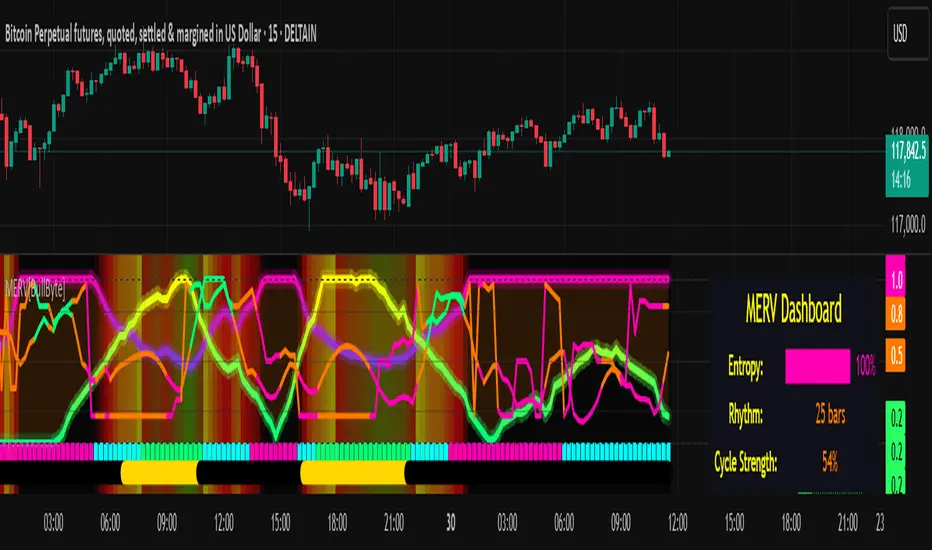
9:45am NIFTY TRADINGTime Frame: 15 Minutes | Reference Candle Time: 9:45 AM IST | Valid Trading Window: 3 Hours
📌 Introduction
This document outlines a structured trading strategy for NIFTY & BANKNIFTY Options based on a 15-minute timeframe with a 9:45 AM IST reference candle. The strategy incorporates technical indicators, probability analysis, and strict trading rules to optimize entries and exits.
📊 Core Features
1. Reference Time Trading System
9:45 AM IST Candle acts as the reference for the day.
All signals (Buy/Sell/Reversal) are generated based on price action relative to this candle.
The valid trading window is 3 hours after the reference candle.
2. Signal Generation Logic
Signal Condition
Buy (B) Price breaks above reference candle high with confirmation
Sell (S) Price breaks below reference candle low with confirmation
Reversal (R) Early trend reversal signal (requires strict confirmation)
3. Probability Analysis System
The strategy calculates Win Probability (%) using 4 components:
Component Weight Calculation
Body Win Probability 30% Based on candle body strength (body % of total range)
Volume Win Probability 30% Current volume vs. average volume strength
Trend Win Probability 40% EMA crossover + RSI momentum alignment
Composite Probability - Weighted average of all 3 components
Probability Color Coding:
🟢 Green (High Probability): ≥70%
🟠 Orange (Medium Probability): 50-69%
🔴 Red (Low Probability): <50%
4. Timeframe Enforcement
Strictly 15-minute charts only (no other timeframes allowed).
System auto-disables signals if the wrong timeframe is selected.
📈 Technical Analysis Components
1. EMA System (Trend Analysis)
Short EMA (9) – Fast trend indicator
Middle EMA (20) – Intermediate trend
Long EMA (50) – Long-term trend confirmation
Rules:
Buy Signal: Price > 9 EMA > 20 EMA > 50 EMA (Bullish trend)
Sell Signal: Price < 9 EMA < 20 EMA < 50 EMA (Bearish trend)
2. Multi-Timeframe RSI (Momentum)
5M, 15M, 1H, 4H, Daily RSI values are compared for divergence/confluence.
Overbought (≥70) / Oversold (≤30) conditions help in reversal signals.
3. Volume Analysis
Volume Strength (%) = (Current Volume / Avg. Volume) × 100
Strong Volume (>120% Avg.) confirms breakout/breakdown.
4. Body Percentage (Candle Strength)
Body % = (Close - Open) / (High - Low) × 100
Strong Bullish Candle: Body > 60%
Strong Bearish Candle: Body < 40%
📊 Visual Elements
1. Information Tables
Reference Data Table (9:45 AM Candle High/Low/Close)
RSI Values Table (5M, 15M, 1H, 4H, Daily)
Signal Legend (Buy/Sell/Reversal indicators)
2. Chart Overlays
Reference Lines (9:45 AM High & Low)
EMA Lines (9, 20, 50)
Signal Labels (B, S, R)
3. Color Coding
High Probability (Green)
Medium Probability (Orange)
Low Probability (Red)
⚠️ Important Usage Guidelines
✅ Best Practices:
Trade only within the 3-hour window (9:45 AM - 12:45 PM IST).
Wait for confirmation (closing above/below reference candle).
Use probability score to filter high-confidence trades.
❌ Avoid:
Trading outside the 15-minute timeframe.
Ignoring volume & RSI divergence.
Overtrading – Stick to 1-2 high-probability setups per day.
🎯 Conclusion
This NIFTY Trading Strategy is optimized for 15-minute charts with a 9:45 AM IST reference candle. It combines EMA trends, RSI momentum, volume analysis, and probability scoring to generate high-confidence signals.
🚀 Key Takeaways:
✔ Reference candle defines the day’s bias.
✔ Probability system filters best trades.
✔ Strict 15M timeframe ensures consistency.
Happy Trading! 📈💰
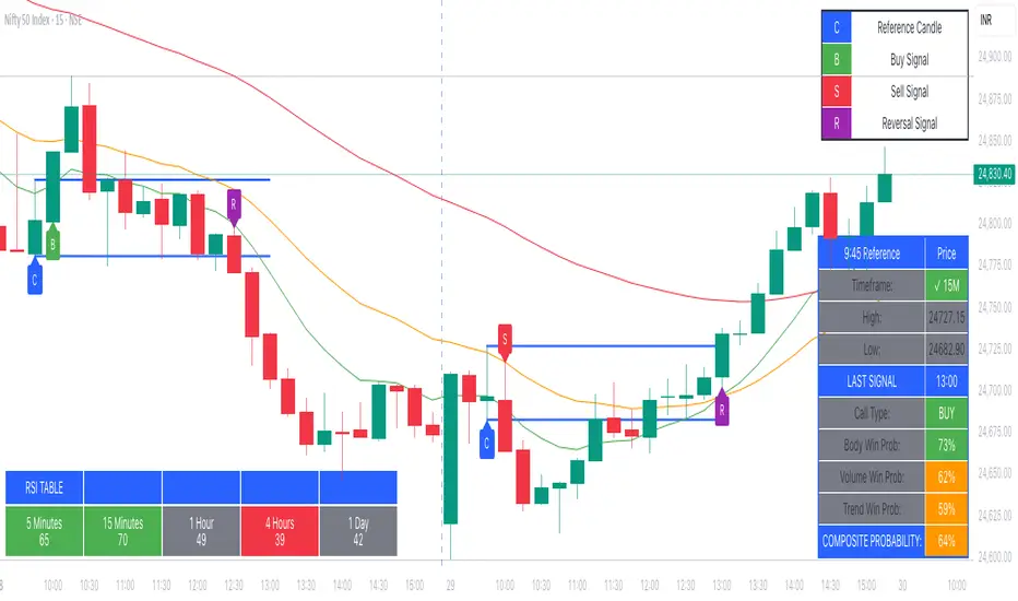
[Mad]Triple Bollinger Bands ForecastTriple Bollinger Bands Forecast (BBx3+F)
This open-source indicator is an advanced version of the classic Bollinger Bands, designed to provide a more comprehensive and forward-looking view of market volatility and potential price levels.
It plots three distinct sets of Bollinger Bands and projects them into the future based on statistical calculations.
How It Is Built and Key Features
Triple Bollinger Bands: Instead of a single set of bands, this indicator plots three. All three share the same central basis line (a Simple Moving Average), but each has a different standard deviation multiplier. This creates three distinct volatility zones for analyzing price deviation from its mean.
Multi-Timeframe (MTF) Capability: The indicator can calculate and display Bollinger Bands from a higher timeframe (e.g., showing daily bands on a 4-hour chart). This allows for contextualizing price action within the volatility structure of a more significant trend.
(Lower HTF selection will result in script-crash!)
Future Forecasting: This is the indicator's main feature. It projects the calculated Bollinger Bands up to 8 bars into the future. This forecast is a recalculation of the Simple Moving Average and Standard Deviation based on a projected future source price.
Selectable Forecast Methods: The mathematical model for estimating the future source price can be selected:
Flat: A model that uses the most recent closing price as the price for all future bars in the calculation window.
Linreg (Linear Regression): A model that calculates a linear regression trend on the last few bars and projects it forward to estimate the future source price.
Efficient Drawing with Polylines: The future projections are drawn on the chart using Pine Script's polyline object. This is an efficient method that draws the forecast data only on the last bar, which avoids repainting issues.
Differences from a Classical Bollinger Bands Indicator
Band Count: A classical indicator shows one set of bands. This indicator plots three sets for a multi-layered view of volatility.
Perspective: Classical Bollinger Bands are purely historical. This indicator is both historical and forward-looking .
Forecasting: The classic version has no forecasting capability. This indicator projects the bands into the future .
Timeframe: The classic version works only on the current timeframe. This indicator has full Multi-Timeframe (MTF) support .
The Mathematics Behind the Future Predictions
The core challenge in forecasting Bollinger Bands is that a future band value depends on future prices, which are unknown. This indicator solves this by simulating a future price series. Here is the step-by-step logic:
Forecast the Source Price for the Next Bar
First, the indicator estimates what the price will be on the next bar.
Flat Method: The forecasted price is the current bar's closing price.
Price_forecast = close
Linreg Method: A linear regression is calculated on the last few bars and extrapolated one step forward.
Price_forecast = ta.linreg(close, linreglen, 1)
Calculate the Future SMA (Basis)
To calculate the Simple Moving Average for the next bar, a new data window is simulated. This window includes the new forecasted price and drops the oldest historical price. For a 1-bar forecast, the calculation is:
SMA_future = (Price_forecast + close + close + ... + close ) / length
Calculate the Future Standard Deviation
Similarly, the standard deviation for the next bar is calculated over this same simulated window of prices, using the new SMA_future as its mean.
// 1. Calculate the sum of squared differences from the new mean
d_f = Price_forecast - SMA_future
d_0 = close - SMA_future
// ... and so on for the rest of the window's prices
SumOfSquares = (d_f)^2 + (d_0)^2 + ... + (d_length-2)^2
// 2. Calculate future variance and then the standard deviation
Var_future = SumOfSquares / length
StDev_future = sqrt(Var_future)
Extending the Forecast (2 to 8 Bars)
For forecasts further into the future (e.g., 2 bars), the script uses the same single Price_forecast for all future steps in the calculation. For a 2-bar forecast, the simulated window effectively contains the forecasted price twice, while dropping the two oldest historical prices. This provides a statistically-grounded projection of where the Bollinger Bands are likely to form.
Usage as a Forecast Extension
This indicator's functionality is designed to be modular. It can be used in conjunction with as example Mad Triple Bollinger Bands MTF script to separate the rendering of historical data from the forward-looking forecast.
Configuration for Combined Use:
Add both the Mad Triple Bollinger Bands MTF and this Triple Bollinger Bands Forecast indicator to your chart.
Open the Settings for this indicator (BBx3+F).
In the 'General Settings' tab, disable the Activate Plotting option.
To ensure data consistency, the Bollinger Length, Multipliers, and Higher Timeframe settings should be identical across both indicators.
This configuration prevents the rendering of duplicate historical bands. The Mad Triple Bollinger Bands MTF script will be responsible for visualizing the historical and current bands, while this script will overlay only the forward-projected polyline data.
Candle Breakout Oscillator [LuxAlgo]The Candle Breakout Oscillator tool allows traders to identify the strength and weakness of the three main market states: bullish, bearish, and choppy.
Know who controls the market at any given moment with an oscillator display with values ranging from 0 to 100 for the three main plots and upper and lower thresholds of 80 and 20 by default.
🔶 USAGE
The Candle Breakout Oscillator represents the three main market states, with values ranging from 0 to 100. By default, the upper and lower thresholds are set at 80 and 20, and when a value exceeds these thresholds, a colored area is displayed for the trader's convenience.
This tool is based on pure price action breakouts. In this context, we understand a breakout as a close above the last candle's high or low, which is representative of market strength. All other close positions in relation to the last candle's limits are considered weakness.
So, when the bullish plot (in green) is at the top of the oscillator (values above 80), it means that the bullish breakouts (close below the last candle low) are at their maximum value over the calculation window, indicating an uptrend. The same interpretation can be made for the bearish plot (in red), indicating a downtrend when high.
On the other hand, weakness is indicated when values are below the lower threshold (20), indicating that breakouts are at their minimum over the last 100 candles. Below are some examples of the possible main interpretations:
There are three main things to look for in this oscillator:
Value reaches extreme
Value leaves extreme
Bullish/Bearish crossovers
As we can see on the chart, before the first crossover happens the bears come out of strength (top) and the bulls come out of weakness (bottom), then after the crossover the bulls reach strength (top) and the bears weakness (bottom), this process is repeated in reverse for the second crossover.
The other main feature of the oscillator is its ability to identify periods of sideways trends when the sideways values have upper readings above 80, and trending behavior when the sideways values have lower readings below 20. As we just saw in the case of bullish vs. bearish, sideways values signal a change in behavior when reaching or leaving the extremes of the oscillator.
🔶 DETAILS
🔹 Data Smoothing
The tool offers up to 10 different smoothing methods. In the chart above, we can see the raw data (smoothing: None) and the RMA, TEMA, or Hull moving averages.
🔹 Data Weighting
Users can add different weighting methods to the data. As we can see in the image above, users can choose between None, Volume, or Price (as in Price Delta for each breakout).
🔶 SETTINGS
Window: Execution window, 100 candles by default
🔹 Data
Smoothing Method: Choose between none or ten moving averages
Smoothing Length: Length for the moving average
Weighting Method: Choose between None, Volume, or Price
🔹 Thresholds
Top: 80 by default
Bottom: 20 by default
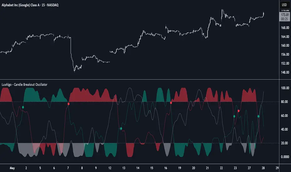
Linear Regression ForecastDescription:
This indicator computes a series of simple linear regressions anchored at the current bar, using look-back windows from 2 bars up to the user-defined maximum. Each regression line is projected forward by the same number of bars as its look-back, producing a family of forecast endpoints. These endpoints are then connected into a continuous polyline: ascending segments are drawn in green, and descending segments in red.
Inputs:
maxLength – Maximum number of bars to include in the longest regression (minimum 2)
priceSource – Price series used for regression (for example, close, open, high, low)
lineWidth – Width of each line segment
Calculation:
For each window size N (from 2 to maxLength):
• Compute least-squares slope and intercept over the N most recent bars (with bar 0 = current bar, bar 1 = one bar ago, etc.).
• Project the regression line to bar_index + N to obtain the forecast price.
Collected forecast points are sorted by projection horizon and then joined:
• First segment: current bar’s price → first forecast point
• Subsequent segments: each forecast point → next forecast point
Segment colors reflect slope direction: green for non-negative, red for negative.
Usage:
Apply this overlay to any price chart. Adjust maxLength to control the depth and reach of the forecast fan. Observe how shorter windows produce nearer-term, more reactive projections, while longer windows yield smoother, more conservative forecasts. Use the colored segments to gauge the overall bias of the fan at each step.
Limitations:
This tool is for informational and educational purposes only. It relies on linear regression assumptions and past price behavior; it does not guarantee future performance. Users should combine it with other technical or fundamental analyses and risk management practices.
LGMM (flat buffers) — multivariate poly + latent statesLGMM POLYNOMIAL BANDS — DISCOVER THE MARKET’S HIDDEN STATES
Overview
Latent-Gaussian-Mixture-Models (LGMMs) view price action as a mix of several invisible regimes: trending up, drifting sideways, sudden volatility spikes, and so on.
A Gaussian Mixture learns these states directly from data and outputs, for every bar, the probability that the market is in each state.
This indicator feeds those probabilities into a rolling polynomial regression that draws a fair-value line, then builds adaptive upper and lower bands.
Band width expands when recent residuals are large *and* when the state mix is uncertain, and contracts when price is calm or one regime clearly dominates.
Crossing back into the band from below generates a buy flag; crossing back into the band from above generates a sell flag (or take-profit for longs).
Key Inputs
Price source – default is Close; you can choose HL2, OHLC4, etc.
Training window (bars) – look-back length for every retrain. 252 bars (one trading year) is a balanced default for US stocks on daily timeframe. Use fewer bars for intraday charts (say 7*24=168 for 1H bars on crypto), more for weekly periods.
Polynomial degree – 1 for a straight trend line, 2 for a curved fit. Curved fits are better when the symbol shows persistent drift.
Hidden states K – number of regimes the mixture tracks (1 to 3). Three states often map well to up-trend, chop, down-trend.
Band width ×σ – multiplier on the entropy-weighted standard deviation. Smaller values (1.5-2) give more trades; larger values (2.5-3) give fewer, higher-conviction trades.
Offline μ,σ pairs (optional) – paste component means and sigmas from an offline LGMM (format: mu1,sigma1;mu2,sigma2;…). Leave blank to let the script use its built-in approximation.
Quick Start
Add the indicator to a chart and wait until the initial Training window has filled.
Watch for green BUY triangles when price closes back above the lower band and red SELL triangles when price closes back below the upper band.
Fine-tune:
– Increase Training window to reduce noise.
– Decrease Band width ×σ for more frequent signals.
– Experiment with Hidden states K; more states capture richer behaviour but need longer windows to stay reliable.
Tips
Bands widen automatically in chaotic periods and tighten when one regime dominates.
Combine with a volume filter or a higher-time-frame trend to reduce whipsaws.
If you already run an LGMM in Python or Matlab, paste its component parameters for a perfect match between your back-test and the TradingView plot.
Works on all markets and time-frames, provided you have at least five times the Training window’s bars in history.
Happy trading!
