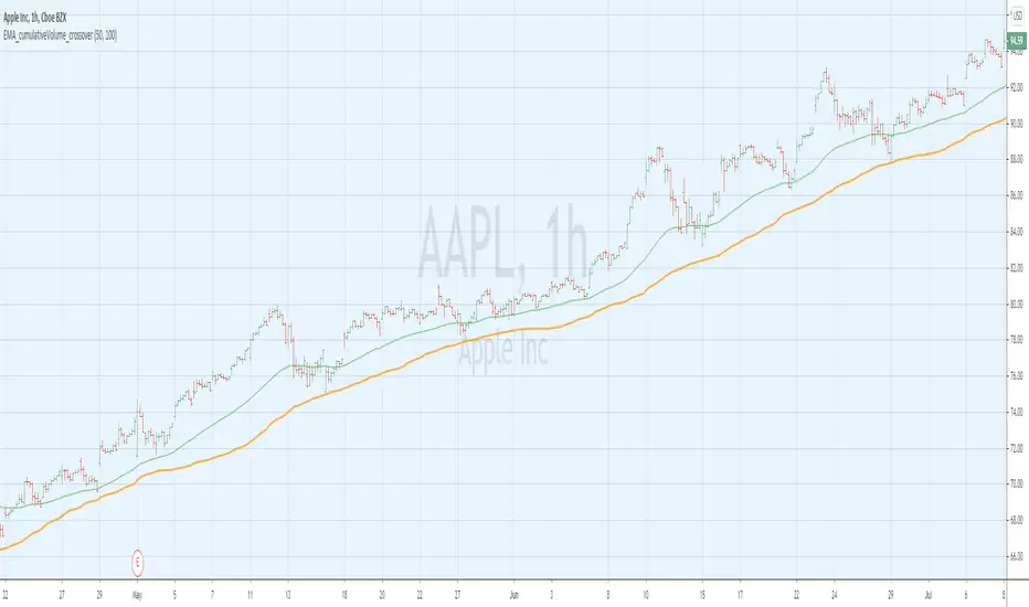
EMA_cumulativeVolume_crossover [indicator]while I was doing some research with exp MA crossovers and volume indicator , I have noticed that when ema 50 is above cumulative volume of 100 period , shows to capture nice profits in that trend. Shorting also (ema50 cross down volume of 100 period) also shows nice results.
BUY
When ema50 crossover cumulative volume of 100 period
Exit
When ema50 cross down cumulative volume of 100 period
Short Selling
Reverse above BUY conditions
Back ground color shows blue when ema50 is above cumulative volume of 100 period, shows purple when ema50 is below cumulative volume of 100 period
I will publish the strategy for back testing later today
Warning
For the use of educational purpose only
Cari dalam skrip untuk "想象图:箱线图+折线组合,横轴为国家,纵轴为响应指数(0-100),箱线显示均值±标准差,叠加红色虚线标注各国确诊高峰时间点"
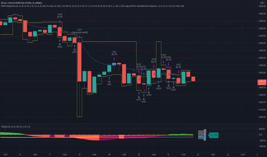
Ruckard TradingLatinoThis strategy tries to mimic TradingLatino strategy.
The current implementation is beta.
Si hablas castellano o espanyol por favor consulta MENSAJE EN CASTELLANO más abajo.
It's aimed at BTCUSDT pair and 4h timeframe.
STRATEGY DEFAULT SETTINGS EXPLANATION
max_bars_back=5000 : This is a random number of bars so that the strategy test lasts for one or two years
calc_on_order_fills=false : To wait for the 4h closing is too much. Try to check if it's worth entering a position after closing one. I finally decided not to recheck if it's worth entering after an order is closed. So it is false.
calc_on_every_tick=false
pyramiding=0 : We only want one entry allowed in the same direction. And we don't want the order to scale by error.
initial_capital=1000 : These are 1000 USDT. By using 1% maximum loss per trade and 7% as a default stop loss by using 1000 USDT at 12000 USDT per BTC price you would entry with around 142 USDT which are converted into: 0.010 BTC . The maximum number of decimal for contracts on this BTCUSDT market is 3 decimals. E.g. the minimum might be: 0.001 BTC . So, this minimal 1000 amount ensures us not to entry with less than 0.001 entries which might have happened when using 100 USDT as an initial capital.
slippage=1 : Binance BTCUSDT mintick is: 0.01. Binance slippage: 0.1 % (Let's assume). TV has an integer slippage. It does not have a percentage based slippage. If we assume a 1000 initial capital, the recommended equity is 142 which at 11996 USDT per BTC price means: 0.011 BTC. The 0.1% slippage of: 0.011 BTC would be: 0.000011 . This is way smaller than the mintick. So our slippage is going to be 1. E.g. 1 (slippage) * 0.01 (mintick)
commission_type=strategy.commission.percent and commission_value=0.1 : According to: binance . com / en / fee / schedule in VIP 0 level both maker and taker fees are: 0.1 %.
BACKGROUND
Jaime Merino is a well known Youtuber focused on crypto trading
His channel TradingLatino
features monday to friday videos where he explains his strategy.
JAIME MERINO STANCE ON BOTS
Jaime Merino stance on bots (taken from memory out of a 2020 June video from him):
'~
You know. They can program you a bot and it might work.
But, there are some special situations that the bot would not be able to handle.
And, I, as a human, I would handle it. And the bot wouldn't do it.
~'
My long term target with this strategy script is add as many
special situations as I can to the script
so that it can match Jaime Merino behaviour even in non normal circumstances.
My alternate target is learn Pine script
and enjoy programming with it.
WARNING
This script might be bigger than other TradingView scripts.
However, please, do not be confused because the current status is beta.
This script has not been tested with real money.
This is NOT an official strategy from Jaime Merino.
This is NOT an official strategy from TradingLatino . net .
HOW IT WORKS
It basically uses ADX slope and LazyBear's Squeeze Momentum Indicator
to make its buy and sell decisions.
Fast paced EMA being bigger than slow paced EMA
(on higher timeframe) advices going long.
Fast paced EMA being smaller than slow paced EMA
(on higher timeframe) advices going short.
It finally add many substrats that TradingLatino uses.
SETTINGS
__ SETTINGS - Basics
____ SETTINGS - Basics - ADX
(ADX) Smoothing {14}
(ADX) DI Length {14}
(ADX) key level {23}
____ SETTINGS - Basics - LazyBear Squeeze Momentum
(SQZMOM) BB Length {20}
(SQZMOM) BB MultFactor {2.0}
(SQZMOM) KC Length {20}
(SQZMOM) KC MultFactor {1.5}
(SQZMOM) Use TrueRange (KC) {True}
____ SETTINGS - Basics - EMAs
(EMAS) EMA10 - Length {10}
(EMAS) EMA10 - Source {close}
(EMAS) EMA55 - Length {55}
(EMAS) EMA55 - Source {close}
____ SETTINGS - Volume Profile
Lowest and highest VPoC from last three days
is used to know if an entry has a support
VPVR of last 100 4h bars
is also taken into account
(VP) Use number of bars (not VP timeframe): Uses 'Number of bars {100}' setting instead of 'Volume Profile timeframe' setting for calculating session VPoC
(VP) Show tick difference from current price {False}: BETA . Might be useful for actions some day.
(VP) Number of bars {100}: If 'Use number of bars (not VP timeframe)' is turned on this setting is used to calculate session VPoC.
(VP) Volume Profile timeframe {1 day}: If 'Use number of bars (not VP timeframe)' is turned off this setting is used to calculate session VPoC.
(VP) Row width multiplier {0.6}: Adjust how the extra Volume Profile bars are shown in the chart.
(VP) Resistances prices number of decimal digits : Round Volume Profile bars label numbers so that they don't have so many decimals.
(VP) Number of bars for bottom VPOC {18}: 18 bars equals 3 days in suggested timeframe of 4 hours. It's used to calculate lowest session VPoC from previous three days. It's also used as a top VPOC for sells.
(VP) Ignore VPOC bottom advice on long {False}: If turned on it ignores bottom VPOC (or top VPOC on sells) when evaluating if a buy entry is worth it.
(VP) Number of bars for VPVR VPOC {100}: Number of bars to calculate the VPVR VPoC. We use 100 as Jaime once used. When the price bounces back to the EMA55 it might just bounce to this VPVR VPoC if its price it's lower than the EMA55 (Sells have inverse algorithm).
____ SETTINGS - ADX Slope
ADX Slope
help us to understand if ADX
has a positive slope, negative slope
or it is rather still.
(ADXSLOPE) ADX cut {23}: If ADX value is greater than this cut (23) then ADX has strength
(ADXSLOPE) ADX minimum steepness entry {45}: ADX slope needs to be 45 degrees to be considered as a positive one.
(ADXSLOPE) ADX minimum steepness exit {45}: ADX slope needs to be -45 degrees to be considered as a negative one.
(ADXSLOPE) ADX steepness periods {3}: In order to avoid false detection the slope is calculated along 3 periods.
____ SETTINGS - Next to EMA55
(NEXTEMA55) EMA10 to EMA55 bounce back percentage {80}: EMA10 might bounce back to EMA55 or maybe to 80% of its complete way to EMA55
(NEXTEMA55) Next to EMA55 percentage {15}: How much next to the EMA55 you need to be to consider it's going to bounce back upwards again.
____ SETTINGS - Stop Loss and Take Profit
You can set a default stop loss or a default take profit.
(STOPTAKE) Stop Loss % {7.0}
(STOPTAKE) Take Profit % {2.0}
____ SETTINGS - Trailing Take Profit
You can customize the default trailing take profit values
(TRAILING) Trailing Take Profit (%) {1.0}: Trailing take profit offset in percentage
(TRAILING) Trailing Take Profit Trigger (%) {2.0}: When 2.0% of benefit is reached then activate the trailing take profit.
____ SETTINGS - MAIN TURN ON/OFF OPTIONS
(EMAS) Ignore advice based on emas {false}.
(EMAS) Ignore advice based on emas (On closing long signal) {False}: Ignore advice based on emas but only when deciding to close a buy entry.
(SQZMOM) Ignore advice based on SQZMOM {false}: Ignores advice based on SQZMOM indicator.
(ADXSLOPE) Ignore advice based on ADX positive slope {false}
(ADXSLOPE) Ignore advice based on ADX cut (23) {true}
(STOPTAKE) Take Profit? {false}: Enables simple Take Profit.
(STOPTAKE) Stop Loss? {True}: Enables simple Stop Loss.
(TRAILING) Enable Trailing Take Profit (%) {True}: Enables Trailing Take Profit.
____ SETTINGS - Strategy mode
(STRAT) Type Strategy: 'Long and Short', 'Long Only' or 'Short Only'. Default: 'Long and Short'.
____ SETTINGS - Risk Management
(RISKM) Risk Management Type: 'Safe', 'Somewhat safe compound' or 'Unsafe compound'. ' Safe ': Calculations are always done with the initial capital (1000) in mind. The maximum losses per trade/day/week/month are taken into account. ' Somewhat safe compound ': Calculations are done with initial capital (1000) or a higher capital if it increases. The maximum losses per trade/day/week/month are taken into account. ' Unsafe compound ': In each order all the current capital is gambled and only the default stop loss per order is taken into account. That means that the maximum losses per trade/day/week/month are not taken into account. Default : 'Somewhat safe compound'.
(RISKM) Maximum loss per trade % {1.0}.
(RISKM) Maximum loss per day % {6.0}.
(RISKM) Maximum loss per week % {8.0}.
(RISKM) Maximum loss per month % {10.0}.
____ SETTINGS - Decimals
(DECIMAL) Maximum number of decimal for contracts {3}: How small (3 decimals means 0.001) an entry position might be in your exchange.
EXTRA 1 - PRICE IS IN RANGE indicator
(PRANGE) Print price is in range {False}: Enable a bottom label that indicates if the price is in range or not.
(PRANGE) Price range periods {5}: How many previous periods are used to calculate the medians
(PRANGE) Price range maximum desviation (%) {0.6} ( > 0 ): Maximum positive desviation for range detection
(PRANGE) Price range minimum desviation (%) {0.6} ( > 0 ): Mininum negative desviation for range detection
EXTRA 2 - SQUEEZE MOMENTUM Desviation indicator
(SQZDIVER) Show degrees {False}: Show degrees of each Squeeze Momentum Divergence lines to the x-axis.
(SQZDIVER) Show desviation labels {False}: Whether to show or not desviation labels for the Squeeze Momentum Divergences.
(SQZDIVER) Show desviation lines {False}: Whether to show or not desviation lines for the Squeeze Momentum Divergences.
EXTRA 3 - VOLUME PROFILE indicator
WARNING: This indicator works not on current bar but on previous bar. So in the worst case it might be VP from 4 hours ago. Don't worry, inside the strategy calculus the correct values are used. It's just that I cannot show the most recent one in the chart.
(VP) Print recent profile {False}: Show Volume Profile indicator
(VP) Avoid label price overlaps {False}: Avoid label prices to overlap on the chart.
EXTRA 4 - ZIGNALY SUPPORT
(ZIG) Zignaly Alert Type {Email}: 'Email', 'Webhook'. ' Email ': Prepare alert_message variable content to be compatible with zignaly expected email content format. ' Webhook ': Prepare alert_message variable content to be compatible with zignaly expected json content format.
EXTRA 5 - DEBUG
(DEBUG) Enable debug on order comments {False}: If set to true it prepares the order message to match the alert_message variable. It makes easier to debug what would have been sent by email or webhook on each of the times an order is triggered.
HOW TO USE THIS STRATEGY
BOT MODE: This is the default setting.
PROPER VOLUME PROFILE VIEWING: Click on this strategy settings. Properties tab. Make sure Recalculate 'each time the order was run' is turned off.
NEWBIE USER: (Check PROPER VOLUME PROFILE VIEWING above!) You might want to turn on the 'Print recent profile {False}' setting. Alternatively you can use my alternate realtime study: 'Resistances and supports based on simplified Volume Profile' but, be aware, it might consume one indicator.
ADVANCED USER 1: Turn on the 'Print price is in range {False}' setting and help us to debug this subindicator. Also help us to figure out how to include this value in the strategy.
ADVANCED USER 2: Turn on the all the (SQZDIVER) settings and help us to figure out how to include this value in the strategy.
ADVANCED USER 3: (Check PROPER VOLUME PROFILE VIEWING above!) Turn on the 'Print recent profile {False}' setting and report any problem with it.
JAIME MERINO: Just use the indicator as it comes by default. It should only show BUY signals, SELL signals and their associated closing signals. From time to time you might want to check 'ADVANCED USER 2' instructions to check that there's actually a divergence. Check also 'ADVANCED USER 1' instructions for your amusement.
EXTRA ADVICE
It's advised that you use this strategy in addition to these two other indicators:
* Squeeze Momentum Indicator
* ADX
so that your chart matches as close as possible to TradingLatino chart.
ZIGNALY INTEGRATION
This strategy supports Zignaly email integration by default. It also supports Zignaly Webhook integration.
ZIGNALY INTEGRATION - Email integration example
What you would write in your alert message:
||{{strategy.order.alert_message}}||key=MYSECRETKEY||
ZIGNALY INTEGRATION - Webhook integration example
What you would write in your alert message:
{ {{strategy.order.alert_message}} , "key" : "MYSECRETKEY" }
CREDITS
I have reused and adapted some code from
'Directional Movement Index + ADX & Keylevel Support' study
which it's from TradingView console user.
I have reused and adapted some code from
'3ema' study
which it's from TradingView hunganhnguyen1193 user.
I have reused and adapted some code from
'Squeeze Momentum Indicator ' study
which it's from TradingView LazyBear user.
I have reused and adapted some code from
'Strategy Tester EMA-SMA-RSI-MACD' study
which it's from TradingView fikira user.
I have reused and adapted some code from
'Support Resistance MTF' study
which it's from TradingView LonesomeTheBlue user.
I have reused and adapted some code from
'TF Segmented Linear Regression' study
which it's from TradingView alexgrover user.
I have reused and adapted some code from
"Poor man's volume profile" study
which it's from TradingView IldarAkhmetgaleev user.
FEEDBACK
Please check the strategy source code for more detailed information
where, among others, I explain all of the substrats
and if they are implemented or not.
Q1. Did I understand wrong any of the Jaime substrats (which I have implemented)?
Q2. The strategy yields quite profit when we should long (EMA10 from 1d timeframe is higher than EMA55 from 1d timeframe.
Why the strategy yields much less profit when we should short (EMA10 from 1d timeframe is lower than EMA55 from 1d timeframe)?
Any idea if you need to do something else rather than just reverse what Jaime does when longing?
FREQUENTLY ASKED QUESTIONS
FAQ1. Why are you giving this strategy for free?
TradingLatino and his fellow enthusiasts taught me this strategy. Now I'm giving back to them.
FAQ2. Seriously! Why are you giving this strategy for free?
I'm confident his strategy might be improved a lot. By keeping it to myself I would avoid other people contributions to improve it.
Now that everyone can contribute this is a win-win.
FAQ3. How can I connect this strategy to my Exchange account?
It seems that you can attach alerts to strategies.
You might want to combine it with a paying account which enable Webhook URLs to work.
I don't know how all of this works right now so I cannot give you advice on it.
You will have to do your own research on this subject. But, be careful. Automating trades, if not done properly,
might end on you automating losses.
FAQ4. I have just found that this strategy by default gives more than 3.97% of 'maximum series of losses'. That's unacceptable according to my risk management policy.
You might want to reduce default stop loss setting from 7% to something like 5% till you are ok with the 'maximum series of losses'.
FAQ5. Where can I learn more about your work on this strategy?
Check the source code. You might find unused strategies. Either because there's not a substantial increases on earnings. Or maybe because they have not been implemented yet.
FAQ6. How much leverage is applied in this strategy?
No leverage.
FAQ7. Any difference with original Jaime Merino strategy?
Most of the times Jaime defines an stop loss at the price entry. That's not the case here. The default stop loss is 7% (but, don't be confused it only means losing 1% of your investment thanks to risk management). There's also a trailing take profit that triggers at 2% profit with a 1% trailing.
FAQ8. Why this strategy return is so small?
The strategy should be improved a lot. And, well, backtesting in this platform is not guaranteed to return theoric results comparable to real-life returns. That's why I'm personally forward testing this strategy to verify it.
MENSAJE EN CASTELLANO
En primer lugar se agradece feedback para mejorar la estrategia.
Si eres un usuario avanzado y quieres colaborar en mejorar el script no dudes en comentar abajo.
Ten en cuenta que aunque toda esta descripción tenga que estar en inglés no es obligatorio que el comentario esté en inglés.
CHISTE - CASTELLANO
¡Pero Jaime!
¡400.000!
¡Tu da mun!
Complex Oscillator [-W-]Eng.
Tradingview in the free version has a limitation - you can only use three indicators on the chart.
Complex Oscillator indicator combines several indicators in one, it is:
- RSI
- Stochastic
- WPR (%R)
- Volumes
The first three are chosen because their values are in the range |0-100| and one scale can be used for them.
The volumes are added because I personally feel sorry to allocate one of the three available places for them. =)
It is much more convenient to use them together with some other indicator.
Volumes also in the range 0-100, that is, they will not show the real numerical value, but only the value relative to the previous volumes.
You can display all the indicators at once or only a few of them.
The chart above shows the same indicator in three different variations.
If you know any other standard indicators with values in the range |0-100|, write in the comments, I will add to this indicator.
Rus.
Tradingview в бесплатной версии имеет ограничение - вы можете использовать только три индикатора на графике.
Индикатор Complex Oscillator объединяет несколько индикаторов в одном, это:
- RSI
- Stochastic
- WPR (%R)
- Volumes
Первые три выбраны из-за того, что их значения лежат в диапазоне |0-100| и для них можно использовать одну шкалу.
Объёмы добавлены, потому что лично мне жалко выделять для них одно из трёх доступных мест. =)
Намного удобнее использовать их вместе с каким-нибудь другим индикатором.
Объёмы относительные, тоже лежат в диапазоне 0-100, то есть реальное численное значение они не покажут, а только величину относительно предыдущих объёмов.
Вы можете вывести показания сразу всех индикаторов или только нескольких из них.
На графике выше представлен один и тот же индикатор в трёх разных вариациях.
Если вы знаете ещё какие-нибудь стандартные индикаторы со значениями в интервале |0-100|, напишите в комментариях, я добавлю в этот индикатор.

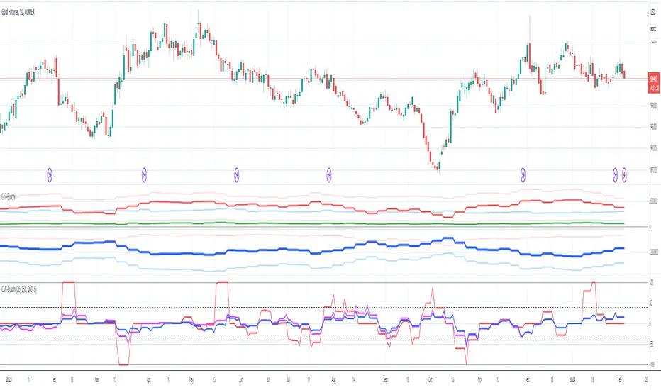
Commercial Movement Index-BuschiEnglish
Inspired by the book "The Commitments of Traders Bible" by Stephen Briese, this indicator is a follow-up of my already published "Commercial Index-Buschi".
Here, the Commercial Index isn't shown in values from 0 to 100, but in how far the value changed from a given timeframe (default Movement Reference: 6 weeks). Therefore it ranges from 100 (bullish move from the Commercials during the last weeks) to -100 (bearish move).
Deutsch
Inspiriert durch das Buch "The Commitments of Traders Bible" by Stephen Briese, ist dieser Indikator eine Weiterentwicklung meines bereits veröffentlichten Skriptes "Commercial Index-Buschi".
Hier wird der Commercial Index nicht in Werten von 0 bis 100 angezeigt, sondern in wieweit er sich innerhalb eines vorgegebenen Zeitfensters (Standard: Movement Reference: 6 Wochen) verändert hat. Daher schwankt er zwischen 100 (bullishe Bewegung der Commercials innerhalb der letzten Wochen) und -100 (bearishe Bewegung).
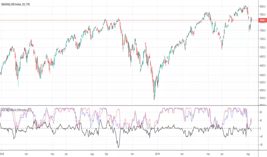
ADL-NDX Rank Difference-Buschi
English:
An expansion of the Advance Decline Line of the NASDAQ. It can be interesting to compare the Advance Decline Line with the corresponding benchmark index. I therefore made a ranking (0 to 100) based on the performance over the last days (default: 21 days). The difference is the target figure and ranges between -100 (bearish divergence) to +100 (bullish divergence).
Deutsch:
Eine Erweiterung der Advance Decline Line der NASDAQ. Oft möchte man den Verlauf der Advance Decline Line mit dem zugehörigen Leitindex vergleichen. Daher habe ich für beide ein Ranking (0 bis 100) erstellt auf Basis des Verlaufs über die letzten Tage (Standardwert: 21 Tage). Die Differenz stellt dabei die Zielgröße dar und schwankt zwischen -100 (bärische Divergenz) und +100 (bullische Divergenz).
ADL-SPX Rank Difference-Buschi
English:
An expansion of the Advance Decline Line of the NYSE. It can be interesting to compare the Advance Decline Line with the corresponding benchmark index. I therefore made a ranking (0 to 100) based on the performance over the last days (default: 21 days). The difference is the target figure and ranges between -100 (bearish divergence) to +100 (bullish divergence).
Deutsch:
Eine Erweiterung der Advance Decline Line der NYSE. Oft möchte man den Verlauf der Advance Decline Line mit dem zugehörigen Leitindex vergleichen. Daher habe ich für beide ein Ranking (0 bis 100) erstellt auf Basis des Verlaufs über die letzten Tage (Standardwert: 21 Tage). Die Differenz stellt dabei die Zielgröße dar und schwankt zwischen -100 (bärische Divergenz) und +100 (bullische Divergenz).

APEX - Aroon / Aroon Oscillator [v1]Simple Script that combines Aroon and Aroon Oscillator with MTF functionality for APEX.
Aroon
The Aroon also know as Aroon Up/Down will help you determine the trend of the asset of if the asset is ranging. The indicator consists of two lines the AroonDown and the Aroon Up.When Aroon Up reaches 100, a new uptrend may have begun. If it remains persistently between 70 and 100, and the Aroon-Down remains between 0 and 30, then a new uptrend is underway.If the Aroon-Up crosses above the Aroon-Down, then a new uptrend may start soon. Conversely, if Aroon-Down crosses above the Aroon-Up, then a new downtrend may start soon. When Aroon-Up reaches 100, a new uptrend may have begun. If it remains persistently between 70 and 100, and the Aroon-Down remains between 0 and 30, then a new uptrend is underway.
Aroon Oscillator
The Aroon Oscillator is the difference between Aroon-Up and Aroon-Down. These two indicators are usually plotted together for easy comparison, but chartists can also view the difference between these two indicators with the Aroon Oscillator. This indicator fluctuates between -100 and +100 with zero as the middle line. An upward trend bias is present when the oscillator is positive, while a downward trend bias exists when the oscillator is negative.

Triple Standard Deviation==日本語説明も併記 // Japanese discription is following ==
■ Momentum Indicator (Triple Indication of Standard Deviation Volatilities)
■ Effective assets: All
■Example of utilization
1) Assume that a trend is generated at the timing when the yellow area chart (26) rises
2) Confirm the candlestick and if the price jumps out of the Bollinger band ± 1 σ, the trend toward that direction
3) If the closing price is confirmed within ± 1σ of the Bollinger band, close the position
■ Detailed explanation
Three standard deviation volatilities with different parameters are displayed at the same time. As represented by convergence divergence of Bollinger, it has a characteristic that it rises in the trend generation period and falls during the trend convergence period.
It develops color in a rising phase so that trend generation is easy to recognize, and fades in a falling phase.
Daily use is basic, but you can use it with the same parameters for other time feet.
The basic parameter (26) is displayed in yellow area for the most visibility.
The long-term parameter (52) is indicated by a yellow dot as an auxiliary element for judging the rising margin of the basic line.
The short-term parameter (13) is displayed as a line as an auxiliary element for recognizing the peak out of the basic line in advance.
In some cases, by changing short term (13) to super long term (100) you can recognize the major market price level once in several years.
Three periods The phrase "all lines" goes from "low position" to "rising together" is considered the strongest trend.
On the other hand, in the case where the short-term line rises backwards as the longer-term line goes down, it tends to end up with short-lived trends and failure to form trends.
If the trend speed is constant as a standard feature of calculating the standard deviation, the standard deviation may decrease even during trend continuation. Therefore, it is desirable to make a comprehensive judgment by comparing the shape of candlestick with the longer-term line.
Please note that there is no way to judge whether the trend suggested by this index rises or falls from this index, so it is necessary to confirm the main chart. (It is preferable to display parabolic or Bollinger band)
■ Remarks
It is an index created assuming that it is used as Triple STD-ADX in combination with Triple Smoothed ADX(to be posted later).
■ About Triple STD-ADX
Triple Standard Deviation "and" Triple Smoothed ADX "are superimposed and displayed as" Screen (without scale) "to function as" Triple STD - ADX ".
The method of utilization is the same as Triple Standard Deviation and Triple Smoothed ADX, but by simultaneously displaying two momentum indicators with different calculation approaches with multiple parameters, we aim to mutually complement the cognitive power of trends.
STD (13, 26, 52, 100, 200) and ADX (7, 14, 26, 52, 100) correspond to reaction rates respectively.
By choosing different reaction rates you can expect to further increase reliability.
You can estimate the reliability of the trend most reliably in a situation where all six signals in total rise from low to high.
■Sample: STD-ADX Trade Signal
========================================================
■ モメンタム指標(標準偏差ボラティリティの3連表示)
■ 有効アセット:すべて
■ 活用の一例
1)黄色のエリアチャート(26)が上昇したタイミングでトレンド発生を想定
2)ローソク足を確認し、ボリンジャーバンド±1σの外に価格が飛び出している場合はその方向へのトレンドと認識
3)ボリンジャーバンド±1σ以内で終値が確定した場合にはポジションクローズ
■ 詳細説明
パラメーターの異なる3つの標準偏差ボラティリティを同時に表示します。ボリンジャーの収束発散に代表されるように、トレンド発生期に上昇しトレンド収束期に低下する特性を持ちます。
トレンド発生を認識しやすいように上昇局面で発色し、下降局面で退色します。
活用は日足が基本ですが、他の時間足に対しても同一パラメーターで使用することができます。
基本パラメーター(26)は最も視認しやすいように黄色のエリア表示にしています。
長期パラメーター(52)は基本線の上昇余力を判断するための補助要素として黄色の丸点で表示しています。
短期パラメーター(13)は基本線のピークアウトを先行して認識するための補助要素としてラインで表示にしています。
場合によって、短期(13)を超長期(100)に変更することで数年に一度のレベルの大相場が認識できます。
3期間「全てのライン」が「低い位置」から「揃って上昇」する局面を最も強いトレンドと考えます。
一方、より長期のラインが低下する中、より短期のラインが逆行して上昇するケースでは、短命のトレンドやトレンド形成失敗に終わることが多くなります。
標準偏差の計算上の特徴としてトレンドの速度が一定の場合にトレンド継続中も標準偏差が低下することがあります。そのため、ローソク足の形状とより長期のラインを見比べて総合的に判断することが望ましいです。
なお、本指標が示唆するトレンドが上昇か下降かは本指標からは判断する術はないため、必ずメインチャートを確認する必要があります。(パラボリックやボリンジャーバンドを表示すると好適)
■備考
追って掲載するTriple Smoothed ADXと併用して、Triple STD-ADXとして使用することを想定して作成した指標です。
■Triple STD-ADXについて
「Triple Standard Deviation」と「Triple Smoothed ADX」を一方を「スクリーン(スケールなし)」として重ねて表示させることで「Triple STD-ADX」として機能します。
活用方法はTriple Standard DeviationやTriple Smoothed ADXと同じですが、算出アプローチの異なる2つのモメンタム指標を複数パラメーターで同時に表示させることで、トレンドの認識力を相互に補完する狙いがあります。
反応速度はそれぞれSTD(13,26,52,100,200)とADX(7,14,26,52,100)がほぼ対応します。
異なる反応速度を選択することで信頼度をさらに高めることを期待できます。
合計6本のシグナル全てが低い位置から揃って上昇する局面でトレンドの信頼性を最も高く見積もることができます。

CCI Multi-TimeframeThe Commodity Channel Index (CCI) is a leading oscillating momentum indicator that was developed by Donald Lambert to identify cyclical turns in commodities but can also be used on securities and bonds as well.
HOW IS IT USED ?
Lambert used the CCI to generate entry and exit signals when the CCI moved above +100% and below -100% respectively. When the CCI moves above +100%, the security enters into a strong uptrend and an entry signal is given. When the CCI moves back below +100% this position should be closed. Conversely, when the CCI moves below -100%, the security enters into a strong downtrend and an exit signal is given. When the CCI moves back above -100% this position should be closed.
In addition, an entry signal is given when the CCI bounces off of the zero line. When the CCI reaches the zero line, the security's average price is at the moving average used to calculate the CCI and when a security bounces off its moving average it is considered a good entry position as the security has pulled back to its short-term support with the bounce reaffirming the current trend.
The CCI can also be used to identify overbought and oversold levels. A security could be considered oversold when the CCI moves below -100 and overbought when it moves above +100. From an oversold level, an entry signal may be given when the CCI moves above -100. From an overbought level, an exit signal might be given when the CCI moves below +100.
Divergences can also be applied to the CCI. A positive divergence below -100 would increase the probability of a signal based on a move above -100, and a negative divergence above +100 would increase the probability of a signal based on a move back below +100.
Trend line breaks can be used to generate entry and exit signals. Trend lines can be drawn connecting the peaks and troughs. From oversold levels, a move above -100 and a trend line breakout could be used as an entry signal. Conversely, from overbought levels, a move below +100 and a trend line breakout could be used as an exit signal.
I added the possibility to add on the chart a 2nd timeframe for confirmation.
If you found this script useful, a tip is always welcome... :)

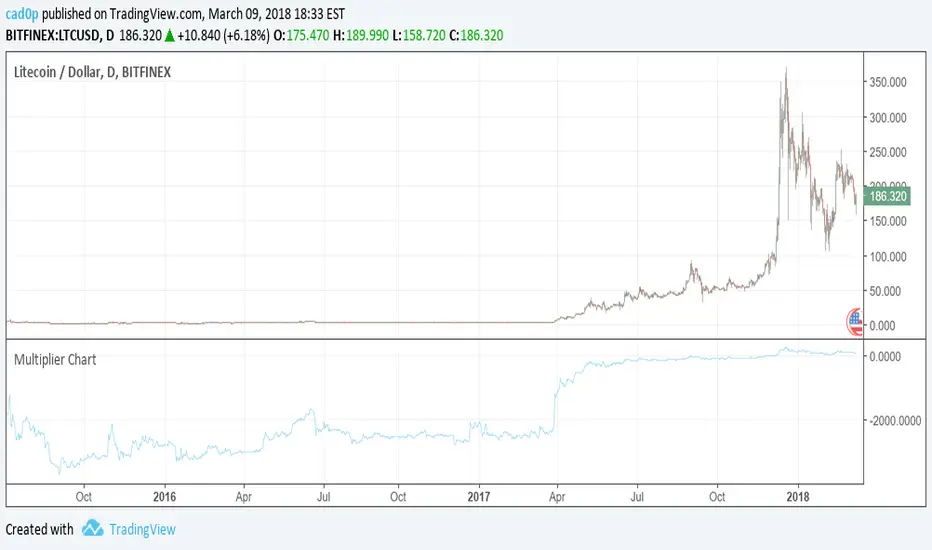
Multiplier ChartI am proposing an alternative to the percent change.
An alternative that is symmetrical to both positive and negative change, unlike percentage change.
The simple idea is to have a positive number if the reference value (called val in the script) is lower than the stock value and needs to be multiplied;
a negative number instead if the reference number is higher than the stock value, so the reference value needs to be divided.
Multiplying all by 100 to give clearer and more readable results, the Multiplier would have a huge gap between +100 and -100, because a stock multiplied by 1 or divided by 1 are the same thing.
So we need to compromise and move all positive numbers down by 100 and all negative numbers up by 100. This actually gives a similar result to percentage change, and it is actually identical in the positive range.
The fundamental difference lies on the negative range, which is completely symmetrical. So if a stock goes up 100 points one day (doubles), and the next it goes down another 100 points (halves), at the end of the second day the stock has the same value as it had at the beginning of the first day! On percentage change it would be +100% the first day and -50% the second.
We mustn't undervalue the human tendency to compare a 1% change to a -1% change, but they do not mean the same even if they seem to indicate so.
A clear example of this can be found on CMC 0.60% -3.56% -3.56% (CoinMarketCap), in which each day are shown the best and worst performing coins of the day. So you might see a +900% there in the top performing, but you'll never see a -900%, because percentage change cannot go further than -100%. It is a fundamentally asymmetric scale that can confuse people a lot especially in those fast moving new markets.ù
I am welcome to feedback and all kinds of opinions and critics.
Some interesting things to note: you can use it as a percentage change indicator or as a different perspective to a stock chart. In fact, it lets you see how big of a difference it made buying coins when they were very cheap, because when they are cheap a difference of what it might seem nothing is amplified by all the gains that the stock/coin made after. So, looking at coins charts using this indicator shows how "not flat" were the early days, which in a normal chart are flattened to 0.
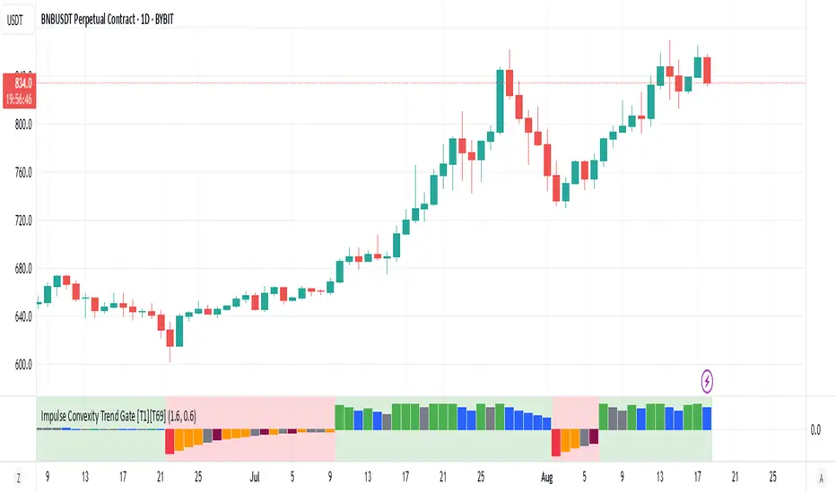
Impulse Convexity Trend Gate [T1][T69]OVERVIEW 🧭
• A price-only trend engine that opens a “gate” only when trend strength, acceleration, and impulse dominance align.
• Built from three cooperating parts: adaptive slope, directional convexity, and an impulse-vs-pullback ratio.
• Output is a bounded oscillator (−100…+100) plus side-specific gate states (bull/bear), with optional pullback and weakness highlights.
THE IDEA & USEFULNESS 🧪
• Not a simple mashup: each component plays a distinct role—slope for direction, convexity for acceleration agreement, and an impulse ratio to suppress correction noise.
• Adaptive EMA length (series-based) lets the midline adjust to conditions without external indicators.
• Approximation of hyperbolic tangent and clamp keep signals bounded and stable while avoiding library dependencies.
• Designed to help trend traders act only when continuation is likely, and stand down during pullbacks or chop.
HOW IT WORKS (PIPELINE) ⚙️
• Price transform
• Uses log price for scale stability.
• Adaptive midline
• Volatility-aware EMA length is clamped between minimum and maximum, then applied via a custom recursive EMA.
• Slope & convexity
• Slope (first difference of the midline) defines direction; convexity (second difference) verifies acceleration agrees with that direction.
• Impulse vs pullback ratio (R)
• Sums directional progress versus counter-direction pullbacks over a window; requires impulse to dominate.
• Normalization & score
• Slope and convexity are normalized by recent dispersion; combined into a raw score and squashed to −100…+100 using manual tanh.
• Trend gate
• Gate opens only when: R ≥ threshold, |normalized slope| ≥ threshold, and slope/convexity share the same sign.
• States & visuals
• Bull/Bear Gate Entry when gate is open, oscillator crosses ±15 in the correct direction, price is on the correct side of the midline, and slope/convexity agree.
• Pullbacks mark counter-moves while a gate is active; Weakness flags specific fade patterns after pullbacks.
FEATURES ✨
• Bull and Bear Gate Entries (green/red columns).
• Pullback shading and optional trend-weakness highlights (yellow/orange + teal/maroon).
• Background tint reflects the active side (bull or bear).
• Pure price logic; no volume or external filters required.
HOW TO USE 🎯
• Regime filter
• Trade only in the direction of the open gate; ignore signals when the gate is closed.
• Pullback entries
• During an open gate, wait for a pullback zone, then act on trend-resumption (e.g., oscillator re-push through ±15 or structure break in gate direction).
• Exits & risk
• Consider trimming when the oscillator relaxes toward 0 while the gate remains open, or when convexity flips against slope and R deteriorates.
• Timeframes & markets
• Suited for trend following on crypto/FX/indices from M30 to 4H/1D; raise thresholds on lower timeframes to reduce noise.
CONFIGURATION 🔧
• Impulse ratio gate (R ≥): raises/lowers the standard for continuation dominance.
• Slope strength gate (|sN| ≥): controls how strong a slope must be to count.
• Show Pullback Impulse (toggle): enable/disable pullback highlights.
• Show Trend Weakness (toggle): enable/disable weakness flags.
LIMITATIONS ⚠️
• As a trend tool, it can lag at regime transitions; expect whipsaws in tight ranges.
• Parameters are instrument- and timeframe-dependent; tune thresholds before live use.
• Pullback/weakness flags are contextual—not trade signals by themselves; use them with gate state and your execution rules.
ADVANCED TIPS 🛠️
• Tighten R and slope thresholds for lower timeframes; loosen for higher timeframes.
• Pair with NNFX-style money management and pair-level filters; let the gate be the confirmation layer, not the entry trigger by itself.
• Batch-test across 100+ symbols, export metrics, and run Monte Carlo to validate LLN reliability and Sharpe/IQR stability.
• For system hedging, disable entries when both sides trigger on the same asset to avoid internal conflict.
NOTES 📝
• Price-only construction reduces data-vendor differences and keeps behavior consistent across markets.
• Manual tanh/clamp ensure stable, bounded scores even during extremes.
DISCLAIMER 🛡️
• For research and education. No financial advice. Test thoroughly, size conservatively, and respect your risk rules.
Stock Profit Calculator — Live Mode
## Overview
This Pine Script indicator calculates, in real time, the financial impact of a stock trade, including purchase/sale commissions, capital gains tax (CGT), and return on investment (ROI). It displays a compact table with key values and also calculates the breakeven price to see at what level the net P/L returns to zero.
---
## Inputs and customization
- **Number of shares:** `shares` defines the purchased quantity.
- **Purchase price:** `buyPrice` is the unit cost; the total purchase is calculated from this.
- **Live selling price:** `sellPrice = close` uses the last bar’s price for live valuation.
- **Fixed or percentage commissions:** `useFixedComm` selects the model.
- **Fixed:** `buyCommFixed`, `sellCommFixed`.
- **Percentage:** `buyCommPct`, `sellCommPct` (applied to notional value).
- **CGT rate:** `cgtRate` is the percentage rate, applied only in case of profit.
- **Table position:** `tablePosition` with predefined options.
- **Visual style:** `colTxt`, `colPos`, `colNeg`, `colBg`, `colHdr`, `colFrame` for text color, positive/negative P/L, background, header, and borders.
> Tip: if your broker uses minimum fees or composite fees, turn on “Use fixed commissions?” and enter the two fixed fees; otherwise, use the percentage model.
---
## Calculation logic
#### Purchase costs
- **Total purchase:**
\
- **Purchase commission:**
\
- **Net entry cost:**
\
#### Sale revenues
- **Total sale (with live price):**
\
- **Sale commission:**
\
- **Net exit revenue:**
\
#### P/L and taxes
- **Gross P/L:**
\
- **CGT (only on positive P/L):**
\
- **Net P/L:**
\
#### ROI
- **Percentage ROI on invested capital:**
\
#### Breakeven
- **Gross breakeven** shown in the table: the unit price that makes the net P/L exactly zero, including purchase cost and an estimate of the sale commission.
\
In the script, if commissions are fixed it adds the fixed sale fee; if percentage-based, the sale component is not included in this row (conservative approximation).
- **Breakeven with tax** (calculated but not shown):
\
Useful when you want the post-CGT result to be exactly zero. Not displayed in the table but ready for use.
> Note: CGT applies only on positive profits; near breakeven, the tax effect is null or only kicks in beyond a threshold. That’s why the script distinguishes between the “gross” and “with tax” versions.
---
## On-screen table
- **Displayed rows:**
- **Purchase:** total net entry cost (with commissions).
- **Sale:** total net exit revenue (with commissions).
- **Gross P/L:** difference between netSell and netBuy.
- **CGT:** estimated tax only if there’s a gain.
- **Net P/L:** P/L after taxes.
- **ROI (%):** percentage return on netBuy.
- **Breakeven:** gross unit breakeven price.
- **Conditional colors:**
- **P/L and ROI:** green for ≥ 0, red for < 0.
- **Headers and cells:** customizable via the color inputs.
- **Efficient refresh:** the table updates only on the last bar via `barstate.islast` to avoid unnecessary redraws.
---
## Behavior and performance
- **Overlay:** displayed on the price chart.
- **Persistent variable:** table is created once with `var table`.
- **Live price:** `sellPrice` follows the current `close`, making P/L, ROI, and breakeven dynamic.
---
## Limitations and suggestions
- **Commission model:** when using percentage commissions, the breakeven in the table doesn’t add the sale percentage fee in the “breakevenPrice” formula. For more precision, you could solve the equation including the percentage fee on exit.
- **Breakeven with tax:** `breakevenWithTax` is a linear estimate; near zero profit, tax may be null. You might choose to display it instead of, or alongside, the gross breakeven.
- **Precision and formatting:** values are shown with `format.mintick`. If the symbol has very small ticks, consider a custom format for better readability.
- **Edge cases:** ROI is undefined if `netBuy = 0` (unlikely in practice but good to note).
> Pro tip: if you want to show the breakeven with tax, add a “Breakeven (post-CGT)” row printing `breakevenWithTax`. If you prefer a single row, replace the shown value with the post-CGT one.
---

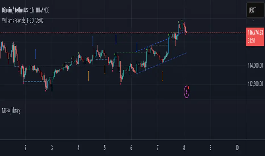
MSFA_LibraryLibrary "MSFA_library"
TODO: add library description here
getDecimals()
Calculates how many decimals are on the quote price of the current market
Returns: The current decimal places on the market quote price
getPipSize(multiplier)
Calculates the pip size of the current market
Parameters:
multiplier (int) : The mintick point multiplier (1 by default, 10 for FX/Crypto/CFD but can be used to override when certain markets require)
Returns: The pip size for the current market
truncate(number, decimalPlaces)
Truncates (cuts) excess decimal places
Parameters:
number (float) : The number to truncate
decimalPlaces (simple float) : (default=2) The number of decimal places to truncate to
Returns: The given number truncated to the given decimalPlaces
toWhole(number)
Converts pips into whole numbers
Parameters:
number (float) : The pip number to convert into a whole number
Returns: The converted number
toPips(number)
Converts whole numbers back into pips
Parameters:
number (float) : The whole number to convert into pips
Returns: The converted number
getPctChange(value1, value2, lookback)
Gets the percentage change between 2 float values over a given lookback period
Parameters:
value1 (float) : The first value to reference
value2 (float) : The second value to reference
lookback (int) : The lookback period to analyze
Returns: The percent change over the two values and lookback period
random(minRange, maxRange)
Wichmann–Hill Pseudo-Random Number Generator
Parameters:
minRange (float) : The smallest possible number (default: 0)
maxRange (float) : The largest possible number (default: 1)
Returns: A random number between minRange and maxRange
bullFib(priceLow, priceHigh, fibRatio)
Calculates a bullish fibonacci value
Parameters:
priceLow (float) : The lowest price point
priceHigh (float) : The highest price point
fibRatio (float) : The fibonacci % ratio to calculate
Returns: The fibonacci value of the given ratio between the two price points
bearFib(priceLow, priceHigh, fibRatio)
Calculates a bearish fibonacci value
Parameters:
priceLow (float) : The lowest price point
priceHigh (float) : The highest price point
fibRatio (float) : The fibonacci % ratio to calculate
Returns: The fibonacci value of the given ratio between the two price points
getMA(length, maType)
Gets a Moving Average based on type (! MUST BE CALLED ON EVERY TICK TO BE ACCURATE, don't place in scopes)
Parameters:
length (simple int) : The MA period
maType (string) : The type of MA
Returns: A moving average with the given parameters
barsAboveMA(lookback, ma)
Counts how many candles are above the MA
Parameters:
lookback (int) : The lookback period to look back over
ma (float) : The moving average to check
Returns: The bar count of how many recent bars are above the MA
barsBelowMA(lookback, ma)
Counts how many candles are below the MA
Parameters:
lookback (int) : The lookback period to look back over
ma (float) : The moving average to reference
Returns: The bar count of how many recent bars are below the EMA
barsCrossedMA(lookback, ma)
Counts how many times the EMA was crossed recently (based on closing prices)
Parameters:
lookback (int) : The lookback period to look back over
ma (float) : The moving average to reference
Returns: The bar count of how many times price recently crossed the EMA (based on closing prices)
getPullbackBarCount(lookback, direction)
Counts how many green & red bars have printed recently (ie. pullback count)
Parameters:
lookback (int) : The lookback period to look back over
direction (int) : The color of the bar to count (1 = Green, -1 = Red)
Returns: The bar count of how many candles have retraced over the given lookback & direction
getBodySize()
Gets the current candle's body size (in POINTS, divide by 10 to get pips)
Returns: The current candle's body size in POINTS
getTopWickSize()
Gets the current candle's top wick size (in POINTS, divide by 10 to get pips)
Returns: The current candle's top wick size in POINTS
getBottomWickSize()
Gets the current candle's bottom wick size (in POINTS, divide by 10 to get pips)
Returns: The current candle's bottom wick size in POINTS
getBodyPercent()
Gets the current candle's body size as a percentage of its entire size including its wicks
Returns: The current candle's body size percentage
isHammer(fib, colorMatch)
Checks if the current bar is a hammer candle based on the given parameters
Parameters:
fib (float) : (default=0.382) The fib to base candle body on
colorMatch (bool) : (default=false) Does the candle need to be green? (true/false)
Returns: A boolean - true if the current bar matches the requirements of a hammer candle
isStar(fib, colorMatch)
Checks if the current bar is a shooting star candle based on the given parameters
Parameters:
fib (float) : (default=0.382) The fib to base candle body on
colorMatch (bool) : (default=false) Does the candle need to be red? (true/false)
Returns: A boolean - true if the current bar matches the requirements of a shooting star candle
isDoji(wickSize, bodySize)
Checks if the current bar is a doji candle based on the given parameters
Parameters:
wickSize (float) : (default=2) The maximum top wick size compared to the bottom (and vice versa)
bodySize (float) : (default=0.05) The maximum body size as a percentage compared to the entire candle size
Returns: A boolean - true if the current bar matches the requirements of a doji candle
isBullishEC(allowance, rejectionWickSize, engulfWick)
Checks if the current bar is a bullish engulfing candle
Parameters:
allowance (float) : (default=0) How many POINTS to allow the open to be off by (useful for markets with micro gaps)
rejectionWickSize (float) : (default=disabled) The maximum rejection wick size compared to the body as a percentage
engulfWick (bool) : (default=false) Does the engulfing candle require the wick to be engulfed as well?
Returns: A boolean - true if the current bar matches the requirements of a bullish engulfing candle
isBearishEC(allowance, rejectionWickSize, engulfWick)
Checks if the current bar is a bearish engulfing candle
Parameters:
allowance (float) : (default=0) How many POINTS to allow the open to be off by (useful for markets with micro gaps)
rejectionWickSize (float) : (default=disabled) The maximum rejection wick size compared to the body as a percentage
engulfWick (bool) : (default=false) Does the engulfing candle require the wick to be engulfed as well?
Returns: A boolean - true if the current bar matches the requirements of a bearish engulfing candle
isInsideBar()
Detects inside bars
Returns: Returns true if the current bar is an inside bar
isOutsideBar()
Detects outside bars
Returns: Returns true if the current bar is an outside bar
barInSession(sess, useFilter)
Determines if the current price bar falls inside the specified session
Parameters:
sess (simple string) : The session to check
useFilter (bool) : (default=true) Whether or not to actually use this filter
Returns: A boolean - true if the current bar falls within the given time session
barOutSession(sess, useFilter)
Determines if the current price bar falls outside the specified session
Parameters:
sess (simple string) : The session to check
useFilter (bool) : (default=true) Whether or not to actually use this filter
Returns: A boolean - true if the current bar falls outside the given time session
dateFilter(startTime, endTime)
Determines if this bar's time falls within date filter range
Parameters:
startTime (int) : The UNIX date timestamp to begin searching from
endTime (int) : the UNIX date timestamp to stop searching from
Returns: A boolean - true if the current bar falls within the given dates
dayFilter(monday, tuesday, wednesday, thursday, friday, saturday, sunday)
Checks if the current bar's day is in the list of given days to analyze
Parameters:
monday (bool) : Should the script analyze this day? (true/false)
tuesday (bool) : Should the script analyze this day? (true/false)
wednesday (bool) : Should the script analyze this day? (true/false)
thursday (bool) : Should the script analyze this day? (true/false)
friday (bool) : Should the script analyze this day? (true/false)
saturday (bool) : Should the script analyze this day? (true/false)
sunday (bool) : Should the script analyze this day? (true/false)
Returns: A boolean - true if the current bar's day is one of the given days
atrFilter(atrValue, maxSize)
Parameters:
atrValue (float)
maxSize (float)
tradeCount()
Calculate total trade count
Returns: Total closed trade count
isLong()
Check if we're currently in a long trade
Returns: True if our position size is positive
isShort()
Check if we're currently in a short trade
Returns: True if our position size is negative
isFlat()
Check if we're currentlyflat
Returns: True if our position size is zero
wonTrade()
Check if this bar falls after a winning trade
Returns: True if we just won a trade
lostTrade()
Check if this bar falls after a losing trade
Returns: True if we just lost a trade
maxDrawdownRealized()
Gets the max drawdown based on closed trades (ie. realized P&L). The strategy tester displays max drawdown as open P&L (unrealized).
Returns: The max drawdown based on closed trades (ie. realized P&L). The strategy tester displays max drawdown as open P&L (unrealized).
totalPipReturn()
Gets the total amount of pips won/lost (as a whole number)
Returns: Total amount of pips won/lost (as a whole number)
longWinCount()
Count how many winning long trades we've had
Returns: Long win count
shortWinCount()
Count how many winning short trades we've had
Returns: Short win count
longLossCount()
Count how many losing long trades we've had
Returns: Long loss count
shortLossCount()
Count how many losing short trades we've had
Returns: Short loss count
breakEvenCount(allowanceTicks)
Count how many break-even trades we've had
Parameters:
allowanceTicks (float) : Optional - how many ticks to allow between entry & exit price (default 0)
Returns: Break-even count
longCount()
Count how many long trades we've taken
Returns: Long trade count
shortCount()
Count how many short trades we've taken
Returns: Short trade count
longWinPercent()
Calculate win rate of long trades
Returns: Long win rate (0-100)
shortWinPercent()
Calculate win rate of short trades
Returns: Short win rate (0-100)
breakEvenPercent(allowanceTicks)
Calculate break even rate of all trades
Parameters:
allowanceTicks (float) : Optional - how many ticks to allow between entry & exit price (default 0)
Returns: Break-even win rate (0-100)
averageRR()
Calculate average risk:reward
Returns: Average winning trade divided by average losing trade
unitsToLots(units)
(Forex) Convert the given unit count to lots (multiples of 100,000)
Parameters:
units (float) : The units to convert into lots
Returns: Units converted to nearest lot size (as float)
skipTradeMonteCarlo(chance, debug)
Checks to see if trade should be skipped to emulate rudimentary Monte Carlo simulation
Parameters:
chance (float) : The chance to skip a trade (0-1 or 0-100, function will normalize to 0-1)
debug (bool) : Whether or not to display a label informing of the trade skip
Returns: True if the trade is skipped, false if it's not skipped (idea being to include this function in entry condition validation checks)
fillCell(tableID, column, row, title, value, bgcolor, txtcolor, tooltip)
This updates the given table's cell with the given values
Parameters:
tableID (table) : The table ID to update
column (int) : The column to update
row (int) : The row to update
title (string) : The title of this cell
value (string) : The value of this cell
bgcolor (color) : The background color of this cell
txtcolor (color) : The text color of this cell
tooltip (string)
Returns: Nothing.
Aetherium Institutional Market Resonance EngineAetherium Institutional Market Resonance Engine (AIMRE)
A Three-Pillar Framework for Decoding Institutional Activity
🎓 THEORETICAL FOUNDATION
The Aetherium Institutional Market Resonance Engine (AIMRE) is a multi-faceted analysis system designed to move beyond conventional indicators and decode the market's underlying structure as dictated by institutional capital flow. Its philosophy is built on a singular premise: significant market moves are preceded by a convergence of context , location , and timing . Aetherium quantifies these three dimensions through a revolutionary three-pillar architecture.
This system is not a simple combination of indicators; it is an integrated engine where each pillar's analysis feeds into a central logic core. A signal is only generated when all three pillars achieve a state of resonance, indicating a high-probability alignment between market organization, key liquidity levels, and cyclical momentum.
⚡ THE THREE-PILLAR ARCHITECTURE
1. 🌌 PILLAR I: THE COHERENCE ENGINE (THE 'CONTEXT')
Purpose: To measure the degree of organization within the market. This pillar answers the question: " Is the market acting with a unified purpose, or is it chaotic and random? "
Conceptual Framework: Institutional campaigns (accumulation or distribution) create a non-random, organized market environment. Retail-driven or directionless markets are characterized by "noise" and chaos. The Coherence Engine acts as a filter to ensure we only engage when institutional players are actively steering the market.
Formulaic Concept:
Coherence = f(Dominance, Synchronization)
Dominance Factor: Calculates the absolute difference between smoothed buying pressure (volume-weighted bullish candles) and smoothed selling pressure (volume-weighted bearish candles), normalized by total pressure. A high value signifies a clear winner between buyers and sellers.
Synchronization Factor: Measures the correlation between the streams of buying and selling pressure over the analysis window. A high positive correlation indicates synchronized, directional activity, while a negative correlation suggests choppy, conflicting action.
The final Coherence score (0-100) represents the percentage of market organization. A high score is a prerequisite for any signal, filtering out unpredictable market conditions.
2. 💎 PILLAR II: HARMONIC LIQUIDITY MATRIX (THE 'LOCATION')
Purpose: To identify and map high-impact institutional footprints. This pillar answers the question: " Where have institutions previously committed significant capital? "
Conceptual Framework: Large institutional orders leave indelible marks on the market in the form of anomalous volume spikes at specific price levels. These are not random occurrences but are areas of intense historical interest. The Harmonic Liquidity Matrix finds these footprints and consolidates them into actionable support and resistance zones called "Harmonic Nodes."
Algorithmic Process:
Footprint Identification: The engine scans the historical lookback period for candles where volume > average_volume * Institutional_Volume_Filter. This identifies statistically significant volume events.
Node Creation: A raw node is created at the mean price of the identified candle.
Dynamic Clustering: The engine uses an ATR-based proximity algorithm. If a new footprint is identified within Node_Clustering_Distance (ATR) of an existing Harmonic Node, it is merged. The node's price is volume-weighted, and its magnitude is increased. This prevents chart clutter and consolidates nearby institutional orders into a single, more significant level.
Node Decay: Nodes that are older than the Institutional_Liquidity_Scanback period are automatically removed from the chart, ensuring the analysis remains relevant to recent market dynamics.
3. 🌊 PILLAR III: CYCLICAL RESONANCE MATRIX (THE 'TIMING')
Purpose: To identify the market's dominant rhythm and its current phase. This pillar answers the question: " Is the market's immediate energy flowing up or down? "
Conceptual Framework: Markets move in waves and cycles of varying lengths. Trading in harmony with the current cyclical phase dramatically increases the probability of success. Aetherium employs a simplified wavelet analysis concept to decompose price action into short, medium, and long-term cycles.
Algorithmic Process:
Cycle Decomposition: The engine calculates three oscillators based on the difference between pairs of Exponential Moving Averages (e.g., EMA8-EMA13 for short cycle, EMA21-EMA34 for medium cycle).
Energy Measurement: The 'energy' of each cycle is determined by its recent volatility (standard deviation). The cycle with the highest energy is designated as the "Dominant Cycle."
Phase Analysis: The engine determines if the dominant cycles are in a bullish phase (rising from a trough) or a bearish phase (falling from a peak).
Cycle Sync: The highest conviction timing signals occur when multiple cycles (e.g., short and medium) are synchronized in the same direction, indicating broad-based momentum.
🔧 COMPREHENSIVE INPUT SYSTEM
Pillar I: Market Coherence Engine
Coherence Analysis Window (10-50, Default: 21): The lookback period for the Coherence Engine.
Lower Values (10-15): Highly responsive to rapid shifts in market control. Ideal for scalping but can be sensitive to noise.
Balanced (20-30): Excellent for day trading, capturing the ebb and flow of institutional sessions.
Higher Values (35-50): Smoother, more stable reading. Best for swing trading and identifying long-term institutional campaigns.
Coherence Activation Level (50-90%, Default: 70%): The minimum market organization required to enable signal generation.
Strict (80-90%): Only allows signals in extremely clear, powerful trends. Fewer, but potentially higher quality signals.
Standard (65-75%): A robust filter that effectively removes choppy conditions while capturing most valid institutional moves.
Lenient (50-60%): Allows signals in less-organized markets. Can be useful in ranging markets but may increase false signals.
Pillar II: Harmonic Liquidity Matrix
Institutional Liquidity Scanback (100-400, Default: 200): How far back the engine looks for institutional footprints.
Short (100-150): Focuses on recent institutional activity, providing highly relevant, immediate levels.
Long (300-400): Identifies major, long-term structural levels. These nodes are often extremely powerful but may be less frequent.
Institutional Volume Filter (1.3-3.0, Default: 1.8): The multiplier for detecting a volume spike.
High (2.5-3.0): Only registers climactic, undeniable institutional volume. Fewer, but more significant nodes.
Low (1.3-1.7): More sensitive, identifying smaller but still relevant institutional interest.
Node Clustering Distance (0.2-0.8 ATR, Default: 0.4): The ATR-based distance for merging nearby nodes.
High (0.6-0.8): Creates wider, more consolidated zones of liquidity.
Low (0.2-0.3): Creates more numerous, precise, and distinct levels.
Pillar III: Cyclical Resonance Matrix
Cycle Resonance Analysis (30-100, Default: 50): The lookback for determining cycle energy and dominance.
Short (30-40): Tunes the engine to faster, shorter-term market rhythms. Best for scalping.
Long (70-100): Aligns the timing component with the larger primary trend. Best for swing trading.
Institutional Signal Architecture
Signal Quality Mode (Professional, Elite, Supreme): Controls the strictness of the three-pillar confluence.
Professional: Loosest setting. May generate signals if two of the three pillars are in strong alignment. Increases signal frequency.
Elite: Balanced setting. Requires a clear, unambiguous resonance of all three pillars. The recommended default.
Supreme: Most stringent. Requires perfect alignment of all three pillars, with each pillar exhibiting exceptionally strong readings (e.g., coherence > 85%). The highest conviction signals.
Signal Spacing Control (5-25, Default: 10): The minimum bars between signals to prevent clutter and redundant alerts.
🎨 ADVANCED VISUAL SYSTEM
The visual architecture of Aetherium is designed not merely for aesthetics, but to provide an intuitive, at-a-glance understanding of the complex data being processed.
Harmonic Liquidity Nodes: The core visual element. Displayed as multi-layered, semi-transparent horizontal boxes.
Magnitude Visualization: The height and opacity of a node's "glow" are proportional to its volume magnitude. More significant nodes appear brighter and larger, instantly drawing the eye to key levels.
Color Coding: Standard nodes are blue/purple, while exceptionally high-magnitude nodes are highlighted in an accent color to denote critical importance.
🌌 Quantum Resonance Field: A dynamic background gradient that visualizes the overall market environment.
Color: Shifts from cool blues/purples (low coherence) to energetic greens/cyans (high coherence and organization), providing instant context.
Intensity: The brightness and opacity of the field are influenced by total market energy (a composite of coherence, momentum, and volume), making powerful market states visually apparent.
💎 Crystalline Lattice Matrix: A geometric web of lines projected from a central moving average.
Mathematical Basis: Levels are projected using multiples of the Golden Ratio (Phi ≈ 1.618) and the ATR. This visualizes the natural harmonic and fractal structure of the market. It is not arbitrary but is based on mathematical principles of market geometry.
🧠 Synaptic Flow Network: A dynamic particle system visualizing the engine's "thought process."
Node Density & Activation: The number of particles and their brightness/color are tied directly to the Market Coherence score. In high-coherence states, the network becomes a dense, bright, and organized web. In chaotic states, it becomes sparse and dim.
⚡ Institutional Energy Waves: Flowing sine waves that visualize market volatility and rhythm.
Amplitude & Speed: The height and speed of the waves are directly influenced by the ATR and volume, providing a feel for market energy.
📊 INSTITUTIONAL CONTROL MATRIX (DASHBOARD)
The dashboard is the central command console, providing a real-time, quantitative summary of each pillar's status.
Header: Displays the script title and version.
Coherence Engine Section:
State: Displays a qualitative assessment of market organization: ◉ PHASE LOCK (High Coherence), ◎ ORGANIZING (Moderate Coherence), or ○ CHAOTIC (Low Coherence). Color-coded for immediate recognition.
Power: Shows the precise Coherence percentage and a directional arrow (↗ or ↘) indicating if organization is increasing or decreasing.
Liquidity Matrix Section:
Nodes: Displays the total number of active Harmonic Liquidity Nodes currently being tracked.
Target: Shows the price level of the nearest significant Harmonic Node to the current price, representing the most immediate institutional level of interest.
Cycle Matrix Section:
Cycle: Identifies the currently dominant market cycle (e.g., "MID ") based on cycle energy.
Sync: Indicates the alignment of the cyclical forces: ▲ BULLISH , ▼ BEARISH , or ◆ DIVERGENT . This is the core timing confirmation.
Signal Status Section:
A unified status bar that provides the final verdict of the engine. It will display "QUANTUM SCAN" during neutral periods, or announce the tier and direction of an active signal (e.g., "◉ TIER 1 BUY ◉" ), highlighted with the appropriate color.
🎯 SIGNAL GENERATION LOGIC
Aetherium's signal logic is built on the principle of strict, non-negotiable confluence.
Condition 1: Context (Coherence Filter): The Market Coherence must be above the Coherence Activation Level. No signals can be generated in a chaotic market.
Condition 2: Location (Liquidity Node Interaction): Price must be actively interacting with a significant Harmonic Liquidity Node.
For a Buy Signal: Price must be rejecting the Node from below (testing it as support).
For a Sell Signal: Price must be rejecting the Node from above (testing it as resistance).
Condition 3: Timing (Cycle Alignment): The Cyclical Resonance Matrix must confirm that the dominant cycles are synchronized with the intended trade direction.
Signal Tiering: The Signal Quality Mode input determines how strictly these three conditions must be met. 'Supreme' mode, for example, might require not only that the conditions are met, but that the Market Coherence is exceptionally high and the interaction with the Node is accompanied by a significant volume spike.
Signal Spacing: A final filter ensures that signals are spaced by a minimum number of bars, preventing over-alerting in a single move.
🚀 ADVANCED TRADING STRATEGIES
The Primary Confluence Strategy: The intended use of the system. Wait for a Tier 1 (Elite/Supreme) or Tier 2 (Professional/Elite) signal to appear on the chart. This represents the alignment of all three pillars. Enter after the signal bar closes, with a stop-loss placed logically on the other side of the Harmonic Node that triggered the signal.
The Coherence Context Strategy: Use the Coherence Engine as a standalone market filter. When Coherence is high (>70%), favor trend-following strategies. When Coherence is low (<50%), avoid new directional trades or favor range-bound strategies. A sharp drop in Coherence during a trend can be an early warning of a trend's exhaustion.
Node-to-Node Trading: In a high-coherence environment, use the Harmonic Liquidity Nodes as both entry points and profit targets. For example, after a BUY signal is generated at one Node, the next Node above it becomes a logical first profit target.
⚖️ RESPONSIBLE USAGE AND LIMITATIONS
Decision Support, Not a Crystal Ball: Aetherium is an advanced decision-support tool. It is designed to identify high-probability conditions based on a model of institutional behavior. It does not predict the future.
Risk Management is Paramount: No indicator can replace a sound risk management plan. Always use appropriate position sizing and stop-losses. The signals provided are probabilistic, not certainties.
Past Performance Disclaimer: The market models used in this script are based on historical data. While robust, there is no guarantee that these patterns will persist in the future. Market conditions can and do change.
Not a "Set and Forget" System: The indicator performs best when its user understands the concepts behind the three pillars. Use the dashboard and visual cues to build a comprehensive view of the market before acting on a signal.
Backtesting is Essential: Before applying this tool to live trading, it is crucial to backtest and forward-test it on your preferred instruments and timeframes to understand its unique behavior and characteristics.
🔮 CONCLUSION
The Aetherium Institutional Market Resonance Engine represents a paradigm shift from single-variable analysis to a holistic, multi-pillar framework. By quantifying the abstract concepts of market context, location, and timing into a unified, logical system, it provides traders with an unprecedented lens into the mechanics of institutional market operations.
It is not merely an indicator, but a complete analytical engine designed to foster a deeper understanding of market dynamics. By focusing on the core principles of institutional order flow, Aetherium empowers traders to filter out market noise, identify key structural levels, and time their entries in harmony with the market's underlying rhythm.
"In all chaos there is a cosmos, in all disorder a secret order." - Carl Jung
— Dskyz, Trade with insight. Trade with confluence. Trade with Aetherium.

RSI of RSI Deviation (RoRD)RSI of RSI Deviation (RoRD) - Advanced Momentum Acceleration Analysis
What is RSI of RSI Deviation (RoRD)?
RSI of RSI Deviation (RoRD) is a insightful momentum indicator that transcends traditional oscillator analysis by measuring the acceleration of momentum through sophisticated mathematical layering. By calculating RSI on RSI itself (RSI²) and applying advanced statistical deviation analysis with T3 smoothing, RoRD reveals hidden market dynamics that single-layer indicators miss entirely.
This isn't just another RSI variant—it's a complete reimagining of how we measure and visualize momentum dynamics. Where traditional RSI shows momentum, RoRD shows momentum's rate of change . Where others show static overbought/oversold levels, RoRD reveals statistically significant deviations unique to each market's character.
Theoretical Foundation - The Mathematics of Momentum Acceleration
1. RSI² (RSI of RSI) - The Core Innovation
Traditional RSI measures price momentum. RoRD goes deeper:
Primary RSI (RSI₁) : Standard RSI calculation on price
Secondary RSI (RSI²) : RSI calculated on RSI₁ values
This creates a "momentum of momentum" indicator that leads price action
Mathematical Expression:
RSI₁ = 100 - (100 / (1 + RS₁))
RSI² = 100 - (100 / (1 + RS₂))
Where RS₂ = Average Gain of RSI₁ / Average Loss of RSI₁
2. T3 Smoothing - Lag-Free Response
The T3 Moving Average, developed by Tim Tillson, provides:
Superior smoothing with minimal lag
Adaptive response through volume factor (vFactor)
Noise reduction while preserving signal integrity
T3 Formula:
T3 = c1×e6 + c2×e5 + c3×e4 + c4×e3
Where e1...e6 are cascaded EMAs and c1...c4 are volume-factor-based coefficients
3. Statistical Z-Score Deviation
RoRD employs dual-layer Z-score normalization :
Initial Z-Score : (RSI² - SMA) / StDev
Final Z-Score : Z-score of the Z-score for refined extremity detection
This identifies statistically rare events relative to recent market behavior
4. Multi-Timeframe Confluence
Compares current timeframe Z-score with higher timeframe (HTF)
Provides directional confirmation across time horizons
Filters false signals through timeframe alignment
Why RoRD is Different & More Sophisticated
Beyond Traditional Indicators:
Acceleration vs. Velocity : While RSI measures momentum (velocity), RoRD measures momentum's rate of change (acceleration)
Adaptive Thresholds : Z-score analysis adapts to market conditions rather than using fixed 70/30 levels
Statistical Significance : Signals are based on mathematical rarity, not arbitrary levels
Leading Indicator : RSI² often turns before price, providing earlier signals
Reduced Whipsaws : T3 smoothing eliminates noise while maintaining responsiveness
Unique Signal Generation:
Quantum Orbs : Multi-layered visual signals for statistically extreme events
Divergence Detection : Automated identification of price/momentum divergences
Regime Backgrounds : Visual market state classification (Bullish/Bearish/Neutral)
Particle Effects : Dynamic visualization of momentum energy
Visual Design & Interpretation Guide
Color Coding System:
Yellow (#e1ff00) : Neutral/balanced momentum state
Red (#ff0000) : Overbought/extreme bullish acceleration
Green (#2fff00) : Oversold/extreme bearish acceleration
Orange : Z-score visualization
Blue : HTF Z-score comparison
Main Visual Elements:
RSI² Line with Glow Effect
Multi-layer glow creates depth and emphasis
Color dynamically shifts based on momentum state
Line thickness indicates signal strength
Quantum Signal Orbs
Green Orbs Below : Statistically rare oversold conditions
Red Orbs Above : Statistically rare overbought conditions
Multiple layers indicate signal strength
Only appear at Z-score extremes for high-conviction signals
Divergence Markers
Green Circles : Bullish divergence detected
Red Circles : Bearish divergence detected
Plotted at pivot points for precision
Background Regimes
Green Background : Bullish momentum regime
Grey Background : Bearish momentum regime
Blue Background : Neutral/transitioning regime
Particle Effects
Density indicates momentum energy
Color matches current RSI² state
Provides dynamic market "feel"
Dashboard Metrics - Deep Dive
RSI² ANALYSIS Section:
RSI² Value (0-100)
Current smoothed RSI of RSI reading
>70 : Strong bullish acceleration
<30 : Strong bearish acceleration
~50 : Neutral momentum state
RSI¹ Value
Traditional RSI for reference
Compare with RSI² for acceleration/deceleration insights
Z-Score Status
🔥 EXTREME HIGH : Z > threshold, statistically rare bullish
❄️ EXTREME LOW : Z < threshold, statistically rare bearish
📈 HIGH/📉 LOW : Elevated but not extreme
➡️ NEUTRAL : Normal statistical range
MOMENTUM Section:
Velocity Indicator
▲▲▲ : Strong positive acceleration
▼▼▼ : Strong negative acceleration
Shows rate of change in RSI²
Strength Bar
██████░░░░ : Visual power gauge
Filled bars indicate momentum strength
Based on deviation from center line
SIGNALS Section:
Divergence Status
🟢 BULLISH DIV : Price making lows, RSI² making highs
🔴 BEARISH DIV : Price making highs, RSI² making lows
⚪ NO DIVERGENCE : No divergence detected
HTF Comparison
🔥 HTF EXTREME : Higher timeframe confirms extremity
📊 HTF NORMAL : Higher timeframe is neutral
Critical for multi-timeframe confirmation
Trading Application & Strategy
Signal Hierarchy (Highest to Lowest Priority):
Quantum Orb + HTF Alignment + Divergence
Highest conviction reversal signal
Z-score extreme + timeframe confluence + divergence
Quantum Orb + HTF Alignment
Strong reversal signal
Wait for price confirmation
Divergence + Regime Change
Medium-term reversal signal
Monitor for orb confirmation
Threshold Crosses
Traditional overbought/oversold
Use as alert, not entry
Entry Strategies:
For Reversals:
Wait for Quantum Orb signal
Confirm with HTF Z-score direction
Enter on price structure break
Stop beyond recent extreme
For Continuations:
Trade with regime background color
Use RSI² pullbacks to center line
Avoid signals against HTF trend
For Scalping:
Focus on Z-score extremes
Quick entries on orb signals
Exit at center line cross
Risk Management:
Reduce position size when signals conflict with HTF
Avoid trades during regime transitions (blue background)
Tighten stops after divergence completion
Scale out at statistical mean reversion
Development & Uniqueness
RoRD represents months of research into momentum dynamics and statistical analysis. Unlike indicators that simply combine existing tools, RoRD introduces several genuine innovations :
True RSI² Implementation : Not a smoothed RSI, but actual RSI calculated on RSI values
Dual Z-Score Normalization : Unique approach to finding statistical extremes
T3 Integration : First RSI² implementation with T3 smoothing for optimal lag reduction
Quantum Orb Visualization : Revolutionary signal display method
Dynamic Regime Detection : Automatic market state classification
Statistical Adaptability : Thresholds adapt to market volatility
This indicator was built from first principles, with each component carefully selected for its mathematical properties and practical trading utility. The result is a professional-grade tool that provides insights unavailable through traditional momentum analysis.
Best Practices & Tips
Start with default settings - they're optimized for most markets
Always check HTF alignment before taking signals
Use divergences as early warning , orbs as confirmation
Respect regime backgrounds - trade with them, not against
Combine with price action - RoRD shows when, price shows where
Adjust Z-score thresholds based on market volatility
Monitor dashboard metrics for complete market context
Conclusion
RoRD isn't just another indicator—it's a complete momentum analysis system that reveals market dynamics invisible to traditional tools. By combining momentum acceleration, statistical analysis, and multi-timeframe confluence with intuitive visualization, RoRD provides traders with a sophisticated edge in any market condition.
Whether you're scalping rapid reversals or positioning for major trend changes, RoRD's unique approach to momentum analysis will transform how you see and trade market dynamics.
See momentum's future. Trade with statistical edge.
Trade with insight. Trade with anticipation.
— Dskyz, for DAFE Trading Systems
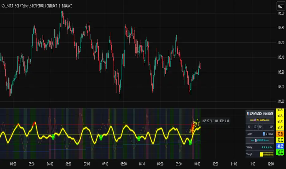
Anomalous Holonomy Field Theory🌌 Anomalous Holonomy Field Theory (AHFT) - Revolutionary Quantum Market Analysis
Where Theoretical Physics Meets Trading Reality
A Groundbreaking Synthesis of Differential Geometry, Quantum Field Theory, and Market Dynamics
🔬 THEORETICAL FOUNDATION - THE MATHEMATICS OF MARKET REALITY
The Anomalous Holonomy Field Theory represents an unprecedented fusion of advanced mathematical physics with practical market analysis. This isn't merely another indicator repackaging old concepts - it's a fundamentally new lens through which to view and understand market structure .
1. HOLONOMY GROUPS (Differential Geometry)
In differential geometry, holonomy measures how vectors change when parallel transported around closed loops in curved space. Applied to markets:
Mathematical Formula:
H = P exp(∮_C A_μ dx^μ)
Where:
P = Path ordering operator
A_μ = Market connection (price-volume gauge field)
C = Closed price path
Market Implementation:
The holonomy calculation measures how price "remembers" its journey through market space. When price returns to a previous level, the holonomy captures what has changed in the market's internal geometry. This reveals:
Hidden curvature in the market manifold
Topological obstructions to arbitrage
Geometric phase accumulated during price cycles
2. ANOMALY DETECTION (Quantum Field Theory)
Drawing from the Adler-Bell-Jackiw anomaly in quantum field theory:
Mathematical Formula:
∂_μ j^μ = (e²/16π²)F_μν F̃^μν
Where:
j^μ = Market current (order flow)
F_μν = Field strength tensor (volatility structure)
F̃^μν = Dual field strength
Market Application:
Anomalies represent symmetry breaking in market structure - moments when normal patterns fail and extraordinary opportunities arise. The system detects:
Spontaneous symmetry breaking (trend reversals)
Vacuum fluctuations (volatility clusters)
Non-perturbative effects (market crashes/melt-ups)
3. GAUGE THEORY (Theoretical Physics)
Markets exhibit gauge invariance - the fundamental physics remains unchanged under certain transformations:
Mathematical Formula:
A'_μ = A_μ + ∂_μΛ
This ensures our signals are gauge-invariant observables , immune to arbitrary market "coordinate changes" like gaps or reference point shifts.
4. TOPOLOGICAL DATA ANALYSIS
Using persistent homology and Morse theory:
Mathematical Formula:
β_k = dim(H_k(X))
Where β_k are the Betti numbers describing topological features that persist across scales.
🎯 REVOLUTIONARY SIGNAL CONFIGURATION
Signal Sensitivity (0.5-12.0, default 2.5)
Controls the responsiveness of holonomy field calculations to market conditions. This parameter directly affects the threshold for detecting quantum phase transitions in price action.
Optimization by Timeframe:
Scalping (1-5min): 1.5-3.0 for rapid signal generation
Day Trading (15min-1H): 2.5-5.0 for balanced sensitivity
Swing Trading (4H-1D): 5.0-8.0 for high-quality signals only
Score Amplifier (10-200, default 50)
Scales the raw holonomy field strength to produce meaningful signal values. Higher values amplify weak signals in low-volatility environments.
Signal Confirmation Toggle
When enabled, enforces additional technical filters (EMA and RSI alignment) to reduce false positives. Essential for conservative strategies.
Minimum Bars Between Signals (1-20, default 5)
Prevents overtrading by enforcing quantum decoherence time between signals. Higher values reduce whipsaws in choppy markets.
👑 ELITE EXECUTION SYSTEM
Execution Modes:
Conservative Mode:
Stricter signal criteria
Higher quality thresholds
Ideal for stable market conditions
Adaptive Mode:
Self-adjusting parameters
Balances signal frequency with quality
Recommended for most traders
Aggressive Mode:
Maximum signal sensitivity
Captures rapid market moves
Best for experienced traders in volatile conditions
Dynamic Position Sizing:
When enabled, the system scales position size based on:
Holonomy field strength
Current volatility regime
Recent performance metrics
Advanced Exit Management:
Implements trailing stops based on ATR and signal strength, with mode-specific multipliers for optimal profit capture.
🧠 ADAPTIVE INTELLIGENCE ENGINE
Self-Learning System:
The strategy analyzes recent trade outcomes and adjusts:
Risk multipliers based on win/loss ratios
Signal weights according to performance
Market regime detection for environmental adaptation
Learning Speed (0.05-0.3):
Controls adaptation rate. Higher values = faster learning but potentially unstable. Lower values = stable but slower adaptation.
Performance Window (20-100 trades):
Number of recent trades analyzed for adaptation. Longer windows provide stability, shorter windows increase responsiveness.
🎨 REVOLUTIONARY VISUAL SYSTEM
1. Holonomy Field Visualization
What it shows: Multi-layer quantum field bands representing market resonance zones
How to interpret:
Blue/Purple bands = Primary holonomy field (strongest resonance)
Band width = Field strength and volatility
Price within bands = Normal quantum state
Price breaking bands = Quantum phase transition
Trading application: Trade reversals at band extremes, breakouts on band violations with strong signals.
2. Quantum Portals
What they show: Entry signals with recursive depth patterns indicating momentum strength
How to interpret:
Upward triangles with portals = Long entry signals
Downward triangles with portals = Short entry signals
Portal depth = Signal strength and expected momentum
Color intensity = Probability of success
Trading application: Enter on portal appearance, with size proportional to portal depth.
3. Field Resonance Bands
What they show: Fibonacci-based harmonic price zones where quantum resonance occurs
How to interpret:
Dotted circles = Minor resonance levels
Solid circles = Major resonance levels
Color coding = Resonance strength
Trading application: Use as dynamic support/resistance, expect reactions at resonance zones.
4. Anomaly Detection Grid
What it shows: Fractal-based support/resistance with anomaly strength calculations
How to interpret:
Triple-layer lines = Major fractal levels with high anomaly probability
Labels show: Period (H8-H55), Price, and Anomaly strength (φ)
⚡ symbol = Extreme anomaly detected
● symbol = Strong anomaly
○ symbol = Normal conditions
Trading application: Expect major moves when price approaches high anomaly levels. Use for precise entry/exit timing.
5. Phase Space Flow
What it shows: Background heatmap revealing market topology and energy
How to interpret:
Dark background = Low market energy, range-bound
Purple glow = Building energy, trend developing
Bright intensity = High energy, strong directional move
Trading application: Trade aggressively in bright phases, reduce activity in dark phases.
📊 PROFESSIONAL DASHBOARD METRICS
Holonomy Field Strength (-100 to +100)
What it measures: The Wilson loop integral around price paths
>70: Strong positive curvature (bullish vortex)
<-70: Strong negative curvature (bearish collapse)
Near 0: Flat connection (range-bound)
Anomaly Level (0-100%)
What it measures: Quantum vacuum expectation deviation
>70%: Major anomaly (phase transition imminent)
30-70%: Moderate anomaly (elevated volatility)
<30%: Normal quantum fluctuations
Quantum State (-1, 0, +1)
What it measures: Market wave function collapse
+1: Bullish eigenstate |↑⟩
0: Superposition (uncertain)
-1: Bearish eigenstate |↓⟩
Signal Quality Ratings
LEGENDARY: All quantum fields aligned, maximum probability
EXCEPTIONAL: Strong holonomy with anomaly confirmation
STRONG: Good field strength, moderate anomaly
MODERATE: Decent signals, some uncertainty
WEAK: Minimal edge, high quantum noise
Performance Metrics
Win Rate: Rolling performance with emoji indicators
Daily P&L: Real-time profit tracking
Adaptive Risk: Current risk multiplier status
Market Regime: Bull/Bear classification
🏆 WHY THIS CHANGES EVERYTHING
Traditional technical analysis operates on 100-year-old principles - moving averages, support/resistance, and pattern recognition. These work because many traders use them, creating self-fulfilling prophecies.
AHFT transcends this limitation by analyzing markets through the lens of fundamental physics:
Markets have geometry - The holonomy calculations reveal this hidden structure
Price has memory - The geometric phase captures path-dependent effects
Anomalies are predictable - Quantum field theory identifies symmetry breaking
Everything is connected - Gauge theory unifies disparate market phenomena
This isn't just a new indicator - it's a new way of thinking about markets . Just as Einstein's relativity revolutionized physics beyond Newton's mechanics, AHFT revolutionizes technical analysis beyond traditional methods.
🔧 OPTIMAL SETTINGS FOR MNQ 10-MINUTE
For the Micro E-mini Nasdaq-100 on 10-minute timeframe:
Signal Sensitivity: 2.5-3.5
Score Amplifier: 50-70
Execution Mode: Adaptive
Min Bars Between: 3-5
Theme: Quantum Nebula or Dark Matter
💭 THE JOURNEY - FROM IMPOSSIBLE THEORY TO TRADING REALITY
Creating AHFT was a mathematical odyssey that pushed the boundaries of what's possible in Pine Script. The journey began with a seemingly impossible question: Could the profound mathematical structures of theoretical physics be translated into practical trading tools?
The Theoretical Challenge:
Months were spent diving deep into differential geometry textbooks, studying the works of Chern, Simons, and Witten. The mathematics of holonomy groups and gauge theory had never been applied to financial markets. Translating abstract mathematical concepts like parallel transport and fiber bundles into discrete price calculations required novel approaches and countless failed attempts.
The Computational Nightmare:
Pine Script wasn't designed for quantum field theory calculations. Implementing the Wilson loop integral, managing complex array structures for anomaly detection, and maintaining computational efficiency while calculating geometric phases pushed the language to its limits. There were moments when the entire project seemed impossible - the script would timeout, produce nonsensical results, or simply refuse to compile.
The Breakthrough Moments:
After countless sleepless nights and thousands of lines of code, breakthrough came through elegant simplifications. The realization that market anomalies follow patterns similar to quantum vacuum fluctuations led to the revolutionary anomaly detection system. The discovery that price paths exhibit holonomic memory unlocked the geometric phase calculations.
The Visual Revolution:
Creating visualizations that could represent 4-dimensional quantum fields on a 2D chart required innovative approaches. The multi-layer holonomy field, recursive quantum portals, and phase space flow representations went through dozens of iterations before achieving the perfect balance of beauty and functionality.
The Balancing Act:
Perhaps the greatest challenge was maintaining mathematical rigor while ensuring practical trading utility. Every formula had to be both theoretically sound and computationally efficient. Every visual had to be both aesthetically pleasing and information-rich.
The result is more than a strategy - it's a synthesis of pure mathematics and market reality that reveals the hidden order within apparent chaos.
📚 INTEGRATED DOCUMENTATION
Once applied to your chart, AHFT includes comprehensive tooltips on every input parameter. The source code contains detailed explanations of the mathematical theory, practical applications, and optimization guidelines. This published description provides the overview - the indicator itself is a complete educational resource.
⚠️ RISK DISCLAIMER
While AHFT employs advanced mathematical models derived from theoretical physics, markets remain inherently unpredictable. No mathematical model, regardless of sophistication, can guarantee future results. This strategy uses realistic commission ($0.62 per contract) and slippage (1 tick) in all calculations. Past performance does not guarantee future results. Always use appropriate risk management and never risk more than you can afford to lose.
🌟 CONCLUSION
The Anomalous Holonomy Field Theory represents a quantum leap in technical analysis - literally. By applying the profound insights of differential geometry, quantum field theory, and gauge theory to market analysis, AHFT reveals structure and opportunities invisible to traditional methods.
From the holonomy calculations that capture market memory to the anomaly detection that identifies phase transitions, from the adaptive intelligence that learns and evolves to the stunning visualizations that make the invisible visible, every component works in mathematical harmony.
This is more than a trading strategy. It's a new lens through which to view market reality.
Trade with the precision of physics. Trade with the power of mathematics. Trade with AHFT.
I hope this serves as a good replacement for Quantum Edge Pro - Adaptive AI until I'm able to fix it.
— Dskyz, Trade with insight. Trade with anticipation.

AWR Pearsons R & LR Oscillator MTF1. Overview
This indicator is designed to analyze the correlation between a price series (or any custom indicator) and the bar index using Pearson’s correlation coefficient. It performs multiple linear regressions over shifted periods and then aggregates these results to create an oscillator. In addition, it integrates a multi-timeframe (MTF) analysis by retrieving the same calculations on 3 different time intervals, providing a more comprehensive view of the trend evolution.
2. User Parameters
The indicator offers several configurable parameters that allow the user to adjust both the calculations and the display:
Source (Linear Regression): The data source on which the regressions are applied (by default, the closing price).
Number of Linear Regressions (numOfLinReg): Allows choosing the number of correlation calculations (up to 10) to be carried out on different shifted periods.
Start Period (startPeriod) and Period Increment (periodIncrement): These parameters define the reference window for each regression. The calculation starts with a base period and then increases with each regression by a fixed increment, creating several time windows to assess the relationship between price evolution and time progression.
Deviation (def_deviation): Although defined, this parameter is intended to control the sensitivity of the calculations. It can be used in further developments of the indicator.
For Multi Time Frames analysis, three additional timeframes are provided through inputs in addition of the current period:
Sum up :
Timeframe 1 = current
Timeframe 2 = 30-minute (default settings)
Timeframe 3 = 1-hour (default settings)
Timeframe 4 = 4-hour (default settings)
These different timeframes allow you to obtain consistent or divergent signals over multiple resolutions, thereby enhancing the confidence of trading decisions.
3. Calculation Logic
At the core of the indicator is the f_calcConditions() function, which performs several essential tasks:
Calculating Pearson's Coefficients For each linear regression, the script uses ta.correlation() to measure the correlation between the chosen source (for example, the closing price) and the chronological index (bar_index). Up to 10 coefficients are computed over shifted windows, providing an evolving view of the linear relationship over different intervals.
Averaging the Results Once the coefficients are calculated, they are stored in an array and averaged to produce a global correlation value called avgPR_local.
Applying Moving Averages
The resulting average is then smoothed using several moving averages (SMA):
A short-term SMA (period of 14),
An intermediate SMA (period of 100),
A long-term SMA (period of 400).
These moving averages help to highlight the underlying trend of the oscillator by indicating the direction in which the correlation is moving.
Defining Trading Conditions Based on avgPR_local and its associated SMAs, multiple conditions are set to generate buy or sell signals:
Simple SMA Conditions :
Small signal :
Light blue below bar signal :
When the averaged coefficients lie between -1 and -0.63, are above the short-term SMA (14 periods), and are increasing, it may indicate a bullish dynamic (buy signal).
Orange above bar signal :
Conversely, when the value is higher (between 0.63 and 1) and below its SMA (14 periods), and are decreasing the trend is considered bearish (sell signal).
Medium signal :
Dark green signal
When the averaged coefficients lie between -1 and -0.45, are above the short-term SMA (14 periods), and are increasing, and also the average 100 is increasing. It may indicate a bullish dynamic (buy signal).
Light red signal :
Conversely, when the value is higher (between 0.45 and 1) and below its SMA (14 periods), the trend and are decreasing, and also the average 100 is decreasing. It may indicate a bearish dynamic(sell signal).
Light green signal :
When the averaged coefficients lie between -1 and -0.15, are above the short-term SMA (14 periods), and are increasing, and also the average 100 & 400 is increasing . It may indicate a bullish dynamic (buy signal).
Dark red signal :
Conversely, when the value is higher (between 0.45 and 1) and below its SMA (14 periods), the trend and are decreasing, and also the average 100 & 400 is decreasing. It may indicate a bearish dynamic(sell signal).
These additional conditions further refine the signals by verifying the consistency of the movement over longer periods. They check that the trends from the respective averages (intermediate and long-term) are in line with the direction indicated by the initial moving average.
These conditions are designed to capture moments when the oscillator's dynamics change, which can be interpreted as opportunities to enter or exit a trade.
4. Multi-Timeframes and Display
One of the main strengths of this indicator is its multi-timeframe approach.
This offers several advantages:
Comparative Analysis: Compare short-term dynamics with broader trends.
Enhanced Signal Reliability: A signal confirmed across multiple timeframes has a higher probability of success.
To visually highlight these signals on the chart, the indicator uses the plotchar() function with distinct symbols for each timeframe:
Current Timeframe: Signals are represented by the character "1"
30-Minute Timeframe: Displayed with the character "2".
1-Hour Timeframe: Displayed with the character "3".
4-Hour Timeframe: Displayed with the character "4".
The colors used are various shades of green for buy signals and shades of red/orange for sell signals, making it easy to distinguish between the different alerts.
5. Integrated Alerts
To avoid missing any trading opportunities, the indicator includes an alert condition via the alertcondition() function. This alert is triggered if any buy or sell signal is generated on any of the analyzed timeframes. The message "MTF valide" indicates that multiple timeframes are confirming the signal, enabling more informed decision-making.
6. How to Use This Indicator
Installation and Configuration: Copy the script into the TradingView Pine Script editor and add it to your chart. The default parameters can be tuned according to market behavior or personal preferences regarding sensitivity and responsiveness.
Interpreting the Signals:
Watch for the symbols on the chart corresponding to each timeframe.
A buy signal appears as a specific symbol below the bar (indicating a bullish condition based on a rising or less negative correlation), while a sell signal appears above the bar.
Multi-Timeframe Analysis: By comparing signals across timeframes, you can filter out false signals. For example, if the short-term timeframe shows a buy signal but the 4-hour timeframe indicates a bearish trend, you may need to reassess your position.
Adjusting the Settings: Depending on the asset type or market volatility, you might need to tweak the periods (startPeriod, periodIncrement) or the number of linear regressions to generate signals that better align with the price dynamics.
Using Alerts: Activate the built-in alert feature so that TradingView notifies you as soon as a multi-timeframe signal is detected. This ensures you stay informed even if you are not continuously monitoring the chart.
In Conclusion
The AWR Pearsons R & LR Oscillator MTF is a powerful tool for traders seeking a detailed understanding of market trends by combining statistical rigor (via Pearson's correlation coefficient) with a multi-timeframe approach. It is capable of generating clear entry and exit signals, visualized with specific symbols and colors depending on the timeframe. By adjusting the parameters to match your trading strategy and leveraging the alert system, you now have a robust instrument for making well-informed market decisions.
Feel free to dive deeper into each component and experiment with different configurations to see how the oscillator integrates with your overall technical analysis strategy. Enjoy exploring its potential and refining your trading approach!

DCA Investment Tracker Pro [tradeviZion]DCA Investment Tracker Pro: Educational DCA Analysis Tool
An educational indicator that helps analyze Dollar-Cost Averaging strategies by comparing actual performance with historical data calculations.
---
💡 Why I Created This Indicator
As someone who practices Dollar-Cost Averaging, I was frustrated with constantly switching between spreadsheets, calculators, and charts just to understand how my investments were really performing. I wanted to see everything in one place - my actual performance, what I should expect based on historical data, and most importantly, visualize where my strategy could take me over the long term .
What really motivated me was watching friends and family underestimate the incredible power of consistent investing. When Napoleon Bonaparte first learned about compound interest, he reportedly exclaimed "I wonder it has not swallowed the world" - and he was right! Yet most people can't visualize how their $500 monthly contributions today could become substantial wealth decades later.
Traditional DCA tracking tools exist, but they share similar limitations:
Require manual data entry and complex spreadsheets
Use fixed assumptions that don't reflect real market behavior
Can't show future projections overlaid on actual price charts
Lose the visual context of what's happening in the market
Make compound growth feel abstract rather than tangible
I wanted to create something different - a tool that automatically analyzes real market history, detects volatility periods, and shows you both current performance AND educational projections based on historical patterns right on your TradingView charts. As Warren Buffett said: "Someone's sitting in the shade today because someone planted a tree a long time ago." This tool helps you visualize your financial tree growing over time.
This isn't just another calculator - it's a visualization tool that makes the magic of compound growth impossible to ignore.
---
🎯 What This Indicator Does
This educational indicator provides DCA analysis tools. Users can input investment scenarios to study:
Theoretical Performance: Educational calculations based on historical return data
Comparative Analysis: Study differences between actual and theoretical scenarios
Historical Projections: Theoretical projections for educational analysis (not predictions)
Performance Metrics: CAGR, ROI, and other analytical metrics for study
Historical Analysis: Calculates historical return data for reference purposes
---
🚀 Key Features
Volatility-Adjusted Historical Return Calculation
Analyzes 3-20 years of actual price data for any symbol
Automatically detects high-volatility stocks (meme stocks, growth stocks)
Uses median returns for volatile stocks, standard CAGR for stable stocks
Provides conservative estimates when extreme outlier years are detected
Smart fallback to manual percentages when data insufficient
Customizable Performance Dashboard
Educational DCA performance analysis with compound growth calculations
Customizable table sizing (Tiny to Huge text options)
9 positioning options (Top/Middle/Bottom + Left/Center/Right)
Theme-adaptive colors (automatically adjusts to dark/light mode)
Multiple display layout options
Future Projection System
Visual future growth projections
Timeframe-aware calculations (Daily/Weekly/Monthly charts)
1-30 year projection options
Shows projected portfolio value and total investment amounts
Investment Insights
Performance vs benchmark comparison
ROI from initial investment tracking
Monthly average return analysis
Investment milestone alerts (25%, 50%, 100% gains)
Contribution tracking and next milestone indicators
---
📊 Step-by-Step Setup Guide
1. Investment Settings 💰
Initial Investment: Enter your starting lump sum (e.g., $60,000)
Monthly Contribution: Set your regular DCA amount (e.g., $500/month)
Return Calculation: Choose "Auto (Stock History)" for real data or "Manual" for fixed %
Historical Period: Select 3-20 years for auto calculations (default: 10 years)
Start Year: When you began investing (e.g., 2020)
Current Portfolio Value: Your actual portfolio worth today (e.g., $150,000)
2. Display Settings 📊
Table Sizes: Choose from Tiny, Small, Normal, Large, or Huge
Table Positions: 9 options - Top/Middle/Bottom + Left/Center/Right
Visibility Toggles: Show/hide Main Table and Stats Table independently
3. Future Projection 🔮
Enable Projections: Toggle on to see future growth visualization
Projection Years: Set 1-30 years ahead for analysis
Live Example - NASDAQ:META Analysis:
Settings shown: $60K initial + $500/month + Auto calculation + 10-year history + 2020 start + $150K current value
---
🔬 Pine Script Code Examples
Core DCA Calculations:
// Calculate total invested over time
months_elapsed = (year - start_year) * 12 + month - 1
total_invested = initial_investment + (monthly_contribution * months_elapsed)
// Compound growth formula for initial investment
theoretical_initial_growth = initial_investment * math.pow(1 + annual_return, years_elapsed)
// Future Value of Annuity for monthly contributions
monthly_rate = annual_return / 12
fv_contributions = monthly_contribution * ((math.pow(1 + monthly_rate, months_elapsed) - 1) / monthly_rate)
// Total expected value
theoretical_total = theoretical_initial_growth + fv_contributions
Volatility Detection Logic:
// Detect extreme years for volatility adjustment
extreme_years = 0
for i = 1 to historical_years
yearly_return = ((price_current / price_i_years_ago) - 1) * 100
if yearly_return > 100 or yearly_return < -50
extreme_years += 1
// Use median approach for high volatility stocks
high_volatility = (extreme_years / historical_years) > 0.2
calculated_return = high_volatility ? median_of_returns : standard_cagr
Performance Metrics:
// Calculate key performance indicators
absolute_gain = actual_value - total_invested
total_return_pct = (absolute_gain / total_invested) * 100
roi_initial = ((actual_value - initial_investment) / initial_investment) * 100
cagr = (math.pow(actual_value / initial_investment, 1 / years_elapsed) - 1) * 100
---
📊 Real-World Examples
See the indicator in action across different investment types:
Stable Index Investments:
AMEX:SPY (SPDR S&P 500) - Shows steady compound growth with standard CAGR calculations
Classic DCA success story: $60K initial + $500/month starting 2020. The indicator shows SPY's historical 10%+ returns, demonstrating how consistent broad market investing builds wealth over time. Notice the smooth theoretical growth line vs actual performance tracking.
MIL:VUAA (Vanguard S&P 500 UCITS) - Shows both data limitation and solution approaches
Data limitation example: VUAA shows "Manual (Auto Failed)" and "No Data" when default 10-year historical setting exceeds available data. The indicator gracefully falls back to manual percentage input while maintaining all DCA calculations and projections.
MIL:VUAA (Vanguard S&P 500 UCITS) - European ETF with successful 5-year auto calculation
Solution demonstration: By adjusting historical period to 5 years (matching available data), VUAA auto calculation works perfectly. Shows how users can optimize settings for newer assets. European market exposure with EUR denomination, demonstrating DCA effectiveness across different markets and currencies.
NYSE:BRK.B (Berkshire Hathaway) - Quality value investment with Warren Buffett's proven track record
Value investing approach: Berkshire Hathaway's legendary performance through DCA lens. The indicator demonstrates how quality companies compound wealth over decades. Lower volatility than tech stocks = standard CAGR calculations used.
High-Volatility Growth Stocks:
NASDAQ:NVDA (NVIDIA Corporation) - Demonstrates volatility-adjusted calculations for extreme price swings
High-volatility example: NVIDIA's explosive AI boom creates extreme years that trigger volatility detection. The indicator automatically switches to "Median (High Vol): 50%" calculations for conservative projections, protecting against unrealistic future estimates based on outlier performance periods.
NASDAQ:TSLA (Tesla) - Shows how 10-year analysis can stabilize volatile tech stocks
Stable long-term growth: Despite Tesla's reputation for volatility, the 10-year historical analysis (34.8% CAGR) shows consistent enough performance that volatility detection doesn't trigger. Demonstrates how longer timeframes can smooth out extreme periods for more reliable projections.
NASDAQ:META (Meta Platforms) - Shows stable tech stock analysis using standard CAGR calculations
Tech stock with stable growth: Despite being a tech stock and experiencing the 2022 crash, META's 10-year history shows consistent enough performance (23.98% CAGR) that volatility detection doesn't trigger. The indicator uses standard CAGR calculations, demonstrating how not all tech stocks require conservative median adjustments.
Notice how the indicator automatically detects high-volatility periods and switches to median-based calculations for more conservative projections, while stable investments use standard CAGR methods.
---
📈 Performance Metrics Explained
Current Portfolio Value: Your actual investment worth today
Expected Value: What you should have based on historical returns (Auto) or your target return (Manual)
Total Invested: Your actual money invested (initial + all monthly contributions)
Total Gains/Loss: Absolute dollar difference between current value and total invested
Total Return %: Percentage gain/loss on your total invested amount
ROI from Initial Investment: How your starting lump sum has performed
CAGR: Compound Annual Growth Rate of your initial investment (Note: This shows initial investment performance, not full DCA strategy)
vs Benchmark: How you're performing compared to the expected returns
---
⚠️ Important Notes & Limitations
Data Requirements: Auto mode requires sufficient historical data (minimum 3 years recommended)
CAGR Limitation: CAGR calculation is based on initial investment growth only, not the complete DCA strategy
Projection Accuracy: Future projections are theoretical and based on historical returns - actual results may vary
Timeframe Support: Works ONLY on Daily (1D), Weekly (1W), and Monthly (1M) charts - no other timeframes supported
Update Frequency: Update "Current Portfolio Value" regularly for accurate tracking
---
📚 Educational Use & Disclaimer
This analysis tool can be applied to various stock and ETF charts for educational study of DCA mathematical concepts and historical performance patterns.
Study Examples: Can be used with symbols like AMEX:SPY , NASDAQ:QQQ , AMEX:VTI , NASDAQ:AAPL , NASDAQ:MSFT , NASDAQ:GOOGL , NASDAQ:AMZN , NASDAQ:TSLA , NASDAQ:NVDA for learning purposes.
EDUCATIONAL DISCLAIMER: This indicator is a study tool for analyzing Dollar-Cost Averaging strategies. It does not provide investment advice, trading signals, or guarantees. All calculations are theoretical examples for educational purposes only. Past performance does not predict future results. Users should conduct their own research and consult qualified financial professionals before making any investment decisions.
---
© 2025 TradeVizion. All rights reserved.
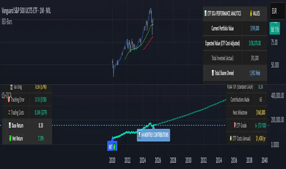
AWR R & LR Oscillator with plots & tableHello trading viewers !
I'm glad to share with you one of my favorite indicator. It's the aggregate of many things. It is partly based on an indicator designed by gentleman goat. Many thanks to him.
1. Oscillator and Correlation Calculations
Overview and Functionality: This part of the indicator computes up to 10 Pearson correlation coefficients between a chosen source (typically the close price, though this is user-configurable) and the bar index over various periods. Starting with an initial period defined by the startPeriod parameter and increasing by a set increment (periodIncrement), each correlation coefficient is calculated using the built-in ta.correlation function over successive ranges. These coefficients are stored in an array, and the indicator calculates their average (avgPR) to provide a complete view of the market trend strength.
Display Features: Each individual coefficient, as well as the overall average, is plotted on the chart using a specific color. Horizontal lines (both dashed and solid) are drawn at levels 0, ±0.8, and ±1, serving as visual thresholds. Additionally, conditional fills in red or blue highlight when values exceed these thresholds, helping the user quickly identify potential extreme conditions (such as overbought or oversold situations).
2. Visual Signals and Automated Alerts
Graphical Signal Enhancements: To reinforce the analysis, the indicator uses graphical elements like emojis and shape markers. For example:
If all 10 curves drop below -0.79, a 🌋 emoji appears at the bottom of the chart;
When curves 2 through 10 are below -0.79, a ⛰️ emoji is displayed below the bar, potentially serving as a buy signal accompanied by an alert condition;
Likewise, symmetrical conditions for correlations exceeding 0.79 produce corresponding emojis (🤿 and 🏖️) at the top or bottom of the chart.
Alerts and Notifications: Using these visual triggers, several alertcondition statements are defined within the script. This allows users to set up TradingView alerts and receive real-time notifications whenever the market reaches these predefined critical zones identified by the multi-period analysis.
3. Regression Channel Analysis
Principles and Calculations: In addition to the oscillator, the indicator implements an analysis of regression channels. For each of the 8 configurable channels, the user can set a range of periods (for example, min1 to max1, etc.). The function calc_regression_channel iterates through the defined period range to find the optimal period that maximizes a statistical measure derived from a regression parameter calculated by the function r(p). Once this optimal period is identified, the indicator computes two key points (A and B) which define the main regression line, and then creates a channel based on the calculated deviation (an RMSE multiplied by a user-defined factor).
The regression channels are not displayed on the chart but are used to plot shapes & fullfilled a table.
Blue shapes are plotted when 6th channel or 7th channel are lower than 3 deviations
Yellow shapes are plotted when 6th channel or 7th channel are higher than 3 deviations
4. Scores, Conditions, and the Summary Table
Scoring System: The indicator goes further by assigning scores across multiple analytical categories, such as:
1. BigPear Score
What It Represents: This score is based on a longer-term moving average of the Pearson correlation values (SMA 100 of the average of the 10 curves of correlation of Pearson). The BigPear category is designed to capture where this longer-term average falls within specific ranges.
Conditions: The script defines nine boolean conditions (labeled BigPear1up through BigPear9up for the “up” direction).
Here's the rules :
BigPear1up = (bigsma_avgPR <= 0.5 and bigsma_avgPR > 0.25)
BigPear2up = (bigsma_avgPR <= 0.25 and bigsma_avgPR > 0)
BigPear3up = (bigsma_avgPR <= 0 and bigsma_avgPR > -0.25)
BigPear4up = (bigsma_avgPR <= -0.25 and bigsma_avgPR > -0.5)
BigPear5up = (bigsma_avgPR <= -0.5 and bigsma_avgPR > -0.65)
BigPear6up = (bigsma_avgPR <= -0.65 and bigsma_avgPR > -0.7)
BigPear7up = (bigsma_avgPR <= -0.7 and bigsma_avgPR > -0.75)
BigPear8up = (bigsma_avgPR <= -0.75 and bigsma_avgPR > -0.8)
BigPear9up = (bigsma_avgPR <= -0.8)
Conditions: The script defines nine boolean conditions (labeled BigPear1down through BigPear9down for the “down” direction).
BigPear1down = (bigsma_avgPR >= -0.5 and bigsma_avgPR < -0.25)
BigPear2down = (bigsma_avgPR >= -0.25 and bigsma_avgPR < 0)
BigPear3down = (bigsma_avgPR >= 0 and bigsma_avgPR < 0.25)
BigPear4down = (bigsma_avgPR >= 0.25 and bigsma_avgPR < 0.5)
BigPear5down = (bigsma_avgPR >= 0.5 and bigsma_avgPR < 0.65)
BigPear6down = (bigsma_avgPR >= 0.65 and bigsma_avgPR < 0.7)
BigPear7down = (bigsma_avgPR >= 0.7 and bigsma_avgPR < 0.75)
BigPear8down = (bigsma_avgPR >= 0.75 and bigsma_avgPR < 0.8)
BigPear9down = (bigsma_avgPR >= 0.8)
Weighting:
If BigPear1up is true, 1 point is added; if BigPear2up is true, 2 points are added; and so on up to 9 points from BigPear9up.
Total Score:
The positive score (posScoreBigPear) is the sum of these weighted conditions.
Similarly, there is a negative score (negScoreBigPear) that is calculated using a mirrored set of conditions (named BigPear1down to BigPear9down), each contributing a negative weight (from -1 to -9).
In essence, the BigPear score tells you—in a weighted cumulative way—where the longer-term correlation average falls relative to predefined thresholds.
2. Pear Score
What It Represents: This category uses the immediate average of the Pearson correlations (avgPR) rather than a longer-term smoothed version. It reflects a more current picture of the market’s correlation behavior.
How It’s Calculated:
Conditions: There are nine conditions defined for the “up” scenario (named Pear1up through Pear9up), which partition the range of avgPR into intervals. For instance:
Pear1up = (avgPR > -0.2 and avgPR <= 0)
Pear2up = (avgPR > -0.4 and avgPR <= -0.2)
Pear3up = (avgPR > -0.5 and avgPR <= -0.4)
Pear4up = (avgPR > -0.6 and avgPR <= -0.5)
Pear5up = (avgPR > -0.65 and avgPR <= -0.6)
Pear6up = (avgPR > -0.7 and avgPR <= -0.65)
Pear7up = (avgPR > -0.75 and avgPR <= -0.7)
Pear8up = (avgPR > -0.8 and avgPR <= -0.75)
Pear9up = (avgPR > -1 and avgPR <= -0.8)
There are nine conditions defined for the “down” scenario (named Pear1down through Pear9down), which partition the range of avgPR into intervals. For instance:
Pear1down = (avgPR >= 0 and avgPR < 0.2)
Pear2down = (avgPR >= 0.2 and avgPR < 0.4)
Pear3down = (avgPR >= 0.4 and avgPR < 0.5)
Pear4down = (avgPR >= 0.5 and avgPR < 0.6)
Pear5down = (avgPR >= 0.6 and avgPR < 0.65)
Pear6down = (avgPR >= 0.65 and avgPR < 0.7)
Pear7down = (avgPR >= 0.7 and avgPR < 0.75)
Pear8down = (avgPR >= 0.75 and avgPR < 0.8)
Pear9down = (avgPR >= 0.8 and avgPR <= 1)
Weighting:
Each condition has an associated weight, such as 0.9 for Pear1up, 1.9 for Pear2up, and so on, up to 9 for Pear9up.
Sum up :
Pear1up = 0.9
Pear2up = 1.9
Pear3up = 2.9
Pear4up = 3.9
Pear5up = 4.99
Pear6up = 6
Pear7up = 7
Pear8up = 8
Pear9up = 9
Total Score:
The positive score (posScorePear) is the sum of these values for each condition that returns true.
A corresponding negative score (negScorePear) is calculated using conditions for when avgPR falls on the positive side, with similar weights in the negative direction.
This score quantifies the current correlation reading by translating its relative level into a numeric score through a weighted sum.
3. Trendpear Score
What It Represents: The Trendpear score is more dynamic as it compares the current avgPR with its short-term moving average (sma_avgPR / 14 periods ) and also considers its relationship with an even longer moving average (bigsma_avgPR / 100 periods). It is meant to capture the trend or momentum in the correlation behavior.
How It’s Calculated:
Conditions: Nine conditions (from Trendpear1up to Trendpear9up) are defined to check:
Whether avgPR is below, equal to, or above sma_avgPR by different margins;
Whether it is trending upward (i.e., it is higher than its previous value).
Here are the rules
Trendpear1up = (avgPR <= sma_avgPR -0.2) and (avgPR >= avgPR )
Trendpear2up = (avgPR > sma_avgPR -0.2) and (avgPR <= sma_avgPR -0.07) and (avgPR >= avgPR )
Trendpear3up = (avgPR > sma_avgPR -0.07) and (avgPR <= sma_avgPR -0.03) and (avgPR >= avgPR )
Trendpear4up = (avgPR > sma_avgPR -0.03) and (avgPR <= sma_avgPR -0.02) and (avgPR >= avgPR )
Trendpear5up = (avgPR > sma_avgPR -0.02) and (avgPR <= sma_avgPR -0.01) and (avgPR >= avgPR )
Trendpear6up = (avgPR > sma_avgPR -0.01) and (avgPR <= sma_avgPR -0.001) and (avgPR >= avgPR )
Trendpear7up = (avgPR >= sma_avgPR) and (avgPR >= avgPR ) and (avgPR <= bigsma_avgPR)
Trendpear8up = (avgPR >= sma_avgPR) and (avgPR >= avgPR ) and (avgPR >= bigsma_avgPR -0.03)
Trendpear9up = (avgPR >= sma_avgPR) and (avgPR >= avgPR ) and (avgPR >= bigsma_avgPR)
Weighting:
The weights here are not linear. For example, the lightest condition may add 0.1 point, whereas the most extreme condition (e.g., when avgPR is not only above the moving average but also reaches a high proportion relative to bigsma_avgPR) might add as much as 90 points.
Trendpear1up = 0.1
Trendpear2up = 0.2
Trendpear3up = 0.3
Trendpear4up = 0.4
Trendpear5up = 0.5
Trendpear6up = 0.69
Trendpear7up = 7
Trendpear8up = 8.9
Trendpear9up = 90
Total Score:
The positive score (posScoreTrendpear) is the sum of the weights from all conditions that are satisfied.
A negative counterpart (negScoreTrendpear) exists similarly for when the trend indicates a downward bias.
Trendpear integrates both the level and the direction of change in the correlations, giving a strong numeric indication when the market starts to diverge from its short-term average.
4. Deviation Score
What It Represents: The “Écart” score quantifies how far the asset’s price deviates from the boundaries defined by the regression channels. This metric can indicate if the price is excessively deviating—which might signal an eventual reversion—or confirming a breakout.
How It’s Calculated:
Conditions: For each channel (with at least seven channels contributing to the scoring from the provided code), there are three levels of deviation:
First tier (EcartXup): Checks if the price is below the upper boundary but above a second boundary.
Second tier (EcartXup2): Checks if the price has dropped further, between a lower and a more extreme boundary.
Third tier (EcartXup3): Checks if the price is below the most extreme limit.
Weighting:
Each tier within a channel has a very small weight for the lowest severities (for example, 0.0001 for the first tier, 0.0002 for the second, 0.0003 for the third) with weights increasing with the channel index.
First channel : 0.0001 to 0.0003 (very short term)
Second channel : 0.001 to 0.003 (short term)
Third channel : 0.01 to 0.03 (short mid term)
4th channel : 0.1 to 0.3 ( mid term)
5th channel: 1 to 3 (long mid term)
6th channel : 10 to 30 (long term)
7th channel : 100 to 300 (very long term)
Total Score:
The overall positive score (posScoreEcart) is the sum of all the weights for conditions met among the first, second, and third tiers.
The corresponding negative score (negScoreEcart) is calculated similarly (using conditions when the price is above the channel boundaries), with the weights being the same in magnitude but negative in sign.
This layered scoring method allows the indicator to reflect both minor and major deviations in a gradated and cumulative manner.
Example :
Score + = 321.0001
Score - = -0.111
The asset price is really overextended in long term view, not for mid term & short term expect the in the very short term.
Score + = 0.0033
Score - = -1.11
The asset price is really extended in short term view, not for mid term (even a bit underextended) & long term is neutral
5. Slope Score
What It Represents: The Slope score captures the trend direction and steepness of the regression channels. It reflects whether the regression line (and hence the underlying trend) is sloping upward or downward.
How It’s Calculated:
Conditions:
if the slope has a uptrend = 1
if the slope has a downtrend = -1
Weighting:
First channel : 0.0001 to 0.0003 (very short term)
Second channel : 0.001 to 0.003 (short term)
Third channel : 0.01 to 0.03 (short mid term)
4th channel : 0.1 to 0.3 ( mid term)
5th channel: 1 to 3 (long mid term)
6th channel : 10 to 30 (long term)
7th channel : 100 to 300 (very long term)
The positive slope conditions incrementally add weights from 0.0001 for the smallest positive slopes to 100 for the largest among the seven checks. And negative for the downward slopes.
The positive score (posScoreSlope) is the sum of all the weights from the upward slope conditions that are met.
The negative score (negScoreSlope) sums the negative weights when downward conditions are met.
Example :
Score + = 111
Score - = -0.1111
Trend is up for longterm & down for mid & short term
The slope score therefore emphasizes both the magnitude and the direction of the trend as indicated by the regression channels, with an intentional asymmetry that flags strong downtrends more aggressively.
Summary
For each category—BigPear, Pear, Trendpear, Écart, and Slope—the indicator evaluates a defined set of conditions. Each condition is a binary test (true/false) based on different thresholds or comparisons (for example, comparing the current value to a moving average or a channel boundary). When a condition is true, its assigned weight is added to the cumulative score for that category. These individual scores, both positive and negative, are then displayed in a table, making it easy for the trader to see at a glance where the market stands according to each analytical dimension.
This comprehensive, weighted approach allows the indicator to encapsulate several layers of market information into a single set of scores, aiding in the identification of potential trading opportunities or market reversals.
5. Practical Use and Application
How to Use the Indicator:
Interpreting the Signals:
On your chart, observe the following components:
The individual correlation curves and their average, plotted with visual thresholds;
Visual markers (such as emojis and shape markers) that signal potential oversold or overbought conditions
The summary table that aggregates the scores from each category, offering a quick glance at the market’s state.
Trading Alerts and Decisions: Set your TradingView alerts through the alertcondition functions provided by the indicator. This way, you receive immediate notifications when critical conditions are met, allowing you to react as soon as the market reaches key levels. This tool is especially beneficial for advanced traders who want to combine multiple technical dimensions to optimize entry and exit points with a confluence of signals.
Conclusion and Additional Insights
In summary, this advanced indicator innovatively combines multi-scale Pearson correlation analysis (via multiple linear regressions) with robust regression channel analysis. It offers a deep and nuanced view of market dynamics by delivering clear visual signals and a comprehensive numerical summary through a built-in score table.
Combine this indicator with other tools (e.g., oscillators, moving averages, volume indicators) to enhance overall strategy robustness.

Mandelbrot-Fibonacci Cascade Vortex (MFCV)Mandelbrot-Fibonacci Cascade Vortex (MFCV) - Where Chaos Theory Meets Sacred Geometry
A Revolutionary Synthesis of Fractal Mathematics and Golden Ratio Dynamics
What began as an exploration into Benoit Mandelbrot's fractal market hypothesis and the mysterious appearance of Fibonacci sequences in nature has culminated in a groundbreaking indicator that reveals the hidden mathematical structure underlying market movements. This indicator represents months of research into chaos theory, fractal geometry, and the golden ratio's manifestation in financial markets.
The Theoretical Foundation
Mandelbrot's Fractal Market Hypothesis Traditional efficient market theory assumes normal distributions and random walks. Mandelbrot proved markets are fractal - self-similar patterns repeating across all timeframes with power-law distributions. The MFCV implements this through:
Hurst Exponent Calculation: H = log(R/S) / log(n/2)
Where:
R = Range of cumulative deviations
S = Standard deviation
n = Period length
This measures market memory:
H > 0.5: Trending (persistent) behavior
H = 0.5: Random walk
H < 0.5: Mean-reverting (anti-persistent) behavior
Fractal Dimension: D = 2 - H
This quantifies market complexity, where higher dimensions indicate more chaotic behavior.
Fibonacci Vortex Theory Markets don't move linearly - they spiral. The MFCV reveals these spirals using Fibonacci sequences:
Vortex Calculation: Vortex(n) = Price + sin(bar_index × φ / Fn) × ATR(Fn) × Volume_Factor
Where:
φ = 0.618 (golden ratio)
Fn = Fibonacci number (8, 13, 21, 34, 55)
Volume_Factor = 1 + (Volume/SMA(Volume,50) - 1) × 0.5
This creates oscillating spirals that contract and expand with market energy.
The Volatility Cascade System
Markets exhibit volatility clustering - Mandelbrot's "Noah Effect." The MFCV captures this through cascading volatility bands:
Cascade Level Calculation: Level(i) = ATR(20) × φ^i
Each level represents a different fractal scale, creating a multi-dimensional view of market structure. The golden ratio spacing ensures harmonic resonance between levels.
Implementation Architecture
Core Components:
Fractal Analysis Engine
Calculates Hurst exponent over user-defined periods
Derives fractal dimension for complexity measurement
Identifies market regime (trending/ranging/chaotic)
Fibonacci Vortex Generator
Creates 5 independent spiral oscillators
Each spiral follows a Fibonacci period
Volume amplification creates dynamic response
Cascade Band System
Up to 8 volatility levels
Golden ratio expansion between levels
Dynamic coloring based on fractal state
Confluence Detection
Identifies convergence of vortex and cascade levels
Highlights high-probability reversal zones
Real-time confluence strength calculation
Signal Generation Logic
The MFCV generates two primary signal types:
Fractal Signals: Generated when:
Hurst > 0.65 (strong trend) AND volatility expanding
Hurst < 0.35 (mean reversion) AND RSI < 35
Trend strength > 0.4 AND vortex alignment
Cascade Signals: Triggered by:
RSI > 60 AND price > SMA(50) AND bearish vortex
RSI < 40 AND price < SMA(50) AND bullish vortex
Volatility expansion AND trend strength > 0.3
Both signals implement a 15-bar cooldown to prevent overtrading.
Advanced Input System
Mandelbrot Parameters:
Cascade Levels (3-8):
Controls number of volatility bands
Crypto: 5-7 (high volatility)
Indices: 4-5 (moderate volatility)
Forex: 3-4 (low volatility)
Hurst Period (20-200):
Lookback for fractal calculation
Scalping: 20-50
Day Trading: 50-100
Swing Trading: 100-150
Position Trading: 150-200
Cascade Ratio (1.0-3.0):
Band width multiplier
1.618: Golden ratio (default)
Higher values for trending markets
Lower values for ranging markets
Fractal Memory (21-233):
Fibonacci retracement lookback
Uses Fibonacci numbers for harmonic alignment
Fibonacci Vortex Settings:
Spiral Periods:
Comma-separated Fibonacci sequence
Fast: "5,8,13,21,34" (scalping)
Standard: "8,13,21,34,55" (balanced)
Extended: "13,21,34,55,89" (swing)
Rotation Speed (0.1-2.0):
Controls spiral oscillation frequency
0.618: Golden ratio (balanced)
Higher = more signals, more noise
Lower = smoother, fewer signals
Volume Amplification:
Enables dynamic spiral expansion
Essential for stocks and crypto
Disable for forex (no central volume)
Visual System Architecture
Cascade Bands:
Multi-level volatility envelopes
Gradient coloring from primary to secondary theme
Transparency increases with distance from price
Fill between bands shows fractal structure
Vortex Spirals:
5 Fibonacci-period oscillators
Blue above price (bullish pressure)
Red below price (bearish pressure)
Multiple display styles: Lines, Circles, Dots, Cross
Dynamic Fibonacci Levels:
Auto-updating retracement levels
Smart update logic prevents disruption near levels
Distance-based transparency (closer = more visible)
Updates every 50 bars or on volatility spikes
Confluence Zones:
Highlighted boxes where indicators converge
Stronger confluence = stronger support/resistance
Key areas for reversal trades
Professional Dashboard System
Main Fractal Dashboard: Displays real-time:
Hurst Exponent with market state
Fractal Dimension with complexity level
Volatility Cascade status
Vortex rotation impact
Market regime classification
Signal strength percentage
Active indicator levels
Vortex Metrics Panel: Shows:
Individual spiral deviations
Convergence/divergence metrics
Real-time vortex positioning
Fibonacci period performance
Fractal Metrics Display: Tracks:
Dimension D value
Market complexity rating
Self-similarity strength
Trend quality assessment
Theory Guide Panel: Educational reference showing:
Mandelbrot principles
Fibonacci vortex concepts
Dynamic trading suggestions
Trading Applications
Trend Following:
High Hurst (>0.65) indicates strong trends
Follow cascade band direction
Use vortex spirals for entry timing
Exit when Hurst drops below 0.5
Mean Reversion:
Low Hurst (<0.35) signals reversal potential
Trade toward vortex spiral convergence
Use Fibonacci levels as targets
Tighten stops in chaotic regimes
Breakout Trading:
Monitor cascade band compression
Watch for vortex spiral alignment
Volatility expansion confirms breakouts
Use confluence zones for targets
Risk Management:
Position size based on fractal dimension
Wider stops in high complexity markets
Tighter stops when Hurst is extreme
Scale out at Fibonacci levels
Market-Specific Optimization
Cryptocurrency:
Cascade Levels: 5-7
Hurst Period: 50-100
Rotation Speed: 0.786-1.2
Enable volume amplification
Stock Indices:
Cascade Levels: 4-5
Hurst Period: 80-120
Rotation Speed: 0.5-0.786
Moderate cascade ratio
Forex:
Cascade Levels: 3-4
Hurst Period: 100-150
Rotation Speed: 0.382-0.618
Disable volume amplification
Commodities:
Cascade Levels: 4-6
Hurst Period: 60-100
Rotation Speed: 0.5-1.0
Seasonal adjustment consideration
Innovation and Originality
The MFCV represents several breakthrough innovations:
First Integration of Mandelbrot Fractals with Fibonacci Vortex Theory
Unique synthesis of chaos theory and sacred geometry
Novel application of Hurst exponent to spiral dynamics
Dynamic Volatility Cascade System
Golden ratio-based band expansion
Multi-timeframe fractal analysis
Self-adjusting to market conditions
Volume-Amplified Vortex Spirals
Revolutionary spiral calculation method
Dynamic response to market participation
Multiple Fibonacci period integration
Intelligent Signal Generation
Cooldown system prevents overtrading
Multi-factor confirmation required
Regime-aware signal filtering
Professional Analytics Dashboard
Institutional-grade metrics display
Real-time fractal analysis
Educational integration
Development Journey
Creating the MFCV involved overcoming numerous challenges:
Mathematical Complexity: Implementing Hurst exponent calculations efficiently
Visual Clarity: Displaying multiple indicators without cluttering
Performance Optimization: Managing array operations and calculations
Signal Quality: Balancing sensitivity with reliability
User Experience: Making complex theory accessible
The result is an indicator that brings PhD-level mathematics to practical trading while maintaining visual elegance and usability.
Best Practices and Guidelines
Start Simple: Use default settings initially
Match Timeframe: Adjust parameters to your trading style
Confirm Signals: Never trade MFCV signals in isolation
Respect Regimes: Adapt strategy to market state
Manage Risk: Use fractal dimension for position sizing
Color Themes
Six professional themes included:
Fractal: Balanced blue/purple palette
Golden: Warm Fibonacci-inspired colors
Plasma: Vibrant modern aesthetics
Cosmic: Dark mode optimized
Matrix: Classic green terminal
Fire: Heat map visualization
Disclaimer
This indicator is for educational and research purposes only. It does not constitute financial advice. While the MFCV reveals deep market structure through advanced mathematics, markets remain inherently unpredictable. Past performance does not guarantee future results.
The integration of Mandelbrot's fractal theory with Fibonacci vortex dynamics provides unique market insights, but should be used as part of a comprehensive trading strategy. Always use proper risk management and never risk more than you can afford to lose.
Acknowledgments
Special thanks to Benoit Mandelbrot for revolutionizing our understanding of markets through fractal geometry, and to the ancient mathematicians who discovered the golden ratio's universal significance.
"The geometry of nature is fractal... Markets are fractal too." - Benoit Mandelbrot
Revealing the Hidden Order in Market Chaos Trade with Mathematical Precision. Trade with MFCV.
— Created with passion for the TradingView community
Trade with insight. Trade with anticipation.
— Dskyz , for DAFE Trading Systems

Enhanced Volume Trend Indicator with BB SqueezeEnhanced Volume Trend Indicator with BB Squeeze: Comprehensive Explanation
The visualization system allows traders to quickly scan multiple securities to identify high-probability setups without detailed analysis of each chart. The progression from squeeze to breakout, supported by volume trend confirmation, offers a systematic approach to identifying trading opportunities.
The script combines multiple technical analysis approaches into a comprehensive dashboard that helps traders make informed decisions by identifying high-probability setups while filtering out noise through its sophisticated confirmation requirements. It combines multiple technical analysis approaches into an integrated visual system that helps traders identify potential trading opportunities while filtering out false signals.
Core Features
1. Volume Analysis Dashboard
The indicator displays various volume-related metrics in customizable tables:
AVOL (After Hours + Pre-Market Volume): Shows extended hours volume as a percentage of the 21-day average volume with color coding for buying/selling pressure. Green indicates buying pressure and red indicates selling pressure.
Volume Metrics: Includes regular volume (VOL), dollar volume ($VOL), relative volume compared to 21-day average (RVOL), and relative volume compared to 90-day average (RVOL90D).
Pre-Market Data: Optional display of pre-market volume (PVOL), pre-market dollar volume (P$VOL), pre-market relative volume (PRVOL), and pre-market price change percentage (PCHG%).
2. Enhanced Volume Trend (VTR) Analysis
The Volume Trend indicator uses adaptive analysis to evaluate buying and selling pressure, combining multiple factors:
MACD (Moving Average Convergence Divergence) components
Volume-to-SMA (Simple Moving Average) ratio
Price direction and market conditions
Volume change rates and momentum
EMA (Exponential Moving Average) alignment and crossovers
Volatility filtering
VTR Visual Indicators
The VTR score ranges from 0-100, with values above 50 indicating bullish conditions and below 50 indicating bearish conditions. This is visually represented by colored circles:
"●" (Filled Circle):
Green: Strong bullish trend (VTR ≥ 80)
Red: Strong bearish trend (VTR ≤ 20)
"◯" (Hollow Circle):
Green: Moderate bullish trend (VTR 65-79)
Red: Moderate bearish trend (VTR 21-35)
"·" (Small Dot):
Green: Weak bullish trend (VTR 55-64)
Red: Weak bearish trend (VTR 36-45)
"○" (Medium Hollow Circle): Neutral conditions (VTR 46-54), shown in gray
In "Both" display mode, the VTR shows both the numerical score (0-100) alongside the appropriate circle symbol.
Enhanced VTR Settings
The Enhanced Volume Trend component offers several advanced customization options:
Adaptive Volume Analysis (volTrendAdaptive):
When enabled, dynamically adjusts volume thresholds based on recent market volatility
Higher volatility periods require proportionally higher volume to generate significant signals
Helps prevent false signals during highly volatile markets
Keep enabled for most trading conditions, especially in volatile markets
Speed of Change Weight (volTrendSpeedWeight, range 0-1):
Controls emphasis on volume acceleration/deceleration rather than absolute levels
Higher values (0.7-1.0): More responsive to new volume trends, better for momentum trading
Lower values (0.2-0.5): Less responsive, better for trend following
Helps identify early volume trends before they fully develop
Momentum Period (volTrendMomentumPeriod, range 2-10):
Defines lookback period for volume change rate calculations
Lower values (2-3): More responsive to recent changes, better for short timeframes
Higher values (7-10): Smoother, better for daily/weekly charts
Directly affects how quickly the indicator responds to new volume patterns
Volatility Filter (volTrendVolatilityFilter):
Adjusts significance of volume by factoring in current price volatility
High volume during high volatility receives less weight
High volume during low volatility receives more weight
Helps distinguish between genuine volume-driven moves and volatility-driven moves
EMA Alignment Weight (volTrendEmaWeight, range 0-1):
Controls importance of EMA alignments in final VTR calculation
Analyzes multiple EMA relationships (5, 10, 21 period)
Higher values (0.7-1.0): Greater emphasis on trend structure
Lower values (0.2-0.5): More focus on pure volume patterns
Display Mode (volTrendDisplayMode):
"Value": Shows only numerical score (0-100)
"Strength": Shows only symbolic representation
"Both": Shows numerical score and symbol together
3. Bollinger Band Squeeze Detection (SQZ)
The BB Squeeze indicator identifies periods of low volatility when Bollinger Bands contract inside Keltner Channels, often preceding significant price movements.
SQZ Visual Indicators
"●" (Filled Circle): Strong squeeze - high probability setup for an impending breakout
Green: Strong squeeze with bullish bias (likely upward breakout)
Red: Strong squeeze with bearish bias (likely downward breakout)
Orange: Strong squeeze with unclear direction
"◯" (Hollow Circle): Moderate squeeze - medium probability setup
Green: With bullish EMA alignment
Red: With bearish EMA alignment
Orange: Without clear directional bias
"-" (Dash): Gray dash indicates no squeeze condition (normal volatility)
The script identifies squeeze conditions through multiple methods:
Bollinger Bands contracting inside Keltner Channels
BB width falling to bottom 20% of recent range (BB width percentile)
Very narrow Keltner Channel (less than 5% of basis price)
Tracking squeeze duration in consecutive bars
Different squeeze strengths are detected:
Strong Squeeze: BB inside KC with tight BB width and narrow KC
Moderate Squeeze: BB inside KC with either tight BB width or narrow KC
No Squeeze: Normal market conditions
4. Breakout Detection System
The script includes two breakout indicators working in sequence:
4.1 Pre-Breakout (PBK) Indicator
Detects potential upcoming breakouts by analyzing multiple factors:
Squeeze conditions lasting 2-3 bars or more
Significant price ranges
Strong volume confirmation
EMA/MACD crossovers
Consistent price direction
PBK Visual Indicators
"●" (Filled Circle): Detected pre-breakout condition
Green: Likely upward breakout (bullish)
Red: Likely downward breakout (bearish)
Orange: Direction not yet clear, but breakout likely
"-" (Dash): Gray dash indicates no pre-breakout condition
The PBK uses sophisticated conditions to reduce false signals including minimum squeeze length, significant price movement, and technical confirmations.
4.2 Breakout (BK) Indicator
Confirms actual breakouts in progress by identifying:
End of squeeze or strong expansion of Bollinger Bands
Volume expansion
Price moving outside Bollinger Bands
EMA crossovers with volume confirmation
MACD crossovers with significant price range
BK Visual Indicators
"●" (Filled Circle): Confirmed breakout in progress
Green: Upward breakout (bullish)
Red: Downward breakout (bearish)
Orange: Unusual breakout pattern without clear direction
"◆" (Diamond): Special breakout conditions (meets some but not all criteria)
"-" (Dash): Gray dash indicates no breakout detected
The BK indicator uses advanced filters for confirmation:
Requires consecutive breakout signals to reduce false positives
Strong volume confirmation requirements (40% above average)
Significant price movement thresholds
Consistency checks between price action and indicators
5. Market Metrics and Analysis
Price Change Percentage (CHG%)
Displays the current percentage change relative to the previous day's close, color-coded green for positive changes and red for negative changes.
Average Daily Range (ADR%)
Calculates the average daily percentage range over a specified period (default 20 days), helping traders gauge volatility and set appropriate price targets.
Average True Range (ATR)
Shows the Average True Range value, a volatility indicator developed by J. Welles Wilder that measures market volatility by decomposing the entire range of an asset price for that period.
Relative Strength Index (RSI)
Displays the standard 14-period RSI, a momentum oscillator that measures the speed and change of price movements on a scale from 0 to 100.
6. External Market Indicators
QQQ Change
Shows the percentage change in the Invesco QQQ Trust (tracking the Nasdaq-100 Index), useful for understanding broader tech market trends.
UVIX Change
Displays the percentage change in UVIX, a volatility index, providing insight into market fear and potential hedging activity.
BTC-USD
Shows the current Bitcoin price from Coinbase, useful for traders monitoring crypto correlation with equities.
Market Breadth (BRD)
Calculates the percentage difference between ATHI.US and ATLO.US (high vs. low securities), indicating overall market direction and strength.
7. Session Analysis and Volume Direction
Session Detection
The script accurately identifies different market sessions:
Pre-market: 4:00 AM to 9:30 AM
Regular market: 9:30 AM to 4:00 PM
After-hours: 4:00 PM to 8:00 PM
Closed: Outside trading hours
This detection works on any timeframe through careful calculation of current time in seconds.
Buy/Sell Volume Direction
The script analyzes buying and selling pressure by:
Counting up volume when close > open
Counting down volume when close < open
Tracking accumulated volume within the day
Calculating intraday pressure (up volume minus down volume)
Enhanced AVOL Calculation
The improved AVOL calculation works in all timeframes by:
Estimating typical pre-market and after-hours volume percentages
Combining yesterday's after-hours with today's pre-market volume
Calculating this as a percentage of the 21-day average volume
Determining buying/selling pressure by analyzing after-hours and pre-market price changes
Color-coding results: green for buying pressure, red for selling pressure
This calculation is particularly valuable because it works consistently across any timeframe.
Customization Options
Display Settings
The dashboard has two customizable tables: Volume Table and Metrics Table, with positions selectable as bottom_left or bottom_right.
All metrics can be individually toggled on/off:
Pre-market data (PVOL, P$VOL, PRVOL, PCHG%)
Volume data (AVOL, RVOL Day, RVOL 90D, Volume, SEED_YASHALGO_NSE_BREADTH:VOLUME )
Price metrics (ADR%, ATR, RSI, Price Change%)
Market indicators (QQQ, UVIX, Breadth, BTC-USD)
Analysis indicators (Volume Trend, BB Squeeze, Pre-Breakout, Breakout)
These toggle options allow traders to customize the dashboard to show only the metrics they find most valuable for their trading style.
Table and Text Customization
The dashboard's appearance can be customized:
Table background color via tableBgColor
Text color (White or Black) via textColorOption
The indicator uses smart formatting for volume and price values, automatically adding appropriate suffixes (K, M, B) for readability.
MACD Configuration for VTR
The Volume Trend calculation incorporates MACD with customizable parameters:
Fast Length: Controls the period for the fast EMA (default 3)
Slow Length: Controls the period for the slow EMA (default 9)
Signal Length: Controls the period for the signal line EMA (default 5)
MACD Weight: Controls how much influence MACD has on the volume trend score (default 0.3)
These settings allow traders to fine-tune how momentum is factored into the volume trend analysis.
Bollinger Bands and Keltner Channel Settings
The Bollinger Bands and Keltner Channels used for squeeze detection have preset (hidden) parameters:
BB Length: 20 periods
BB Multiplier: 2.0 standard deviations
Keltner Length: 20 periods
Keltner Multiplier: 1.5 ATR
These settings follow standard practice for squeeze detection while maintaining simplicity in the user interface.
Practical Trading Applications
Complete Trading Strategies
1. Squeeze Breakout Strategy
This strategy combines multiple components of the indicator:
Wait for a strong squeeze (SQZ showing ●)
Look for pre-breakout confirmation (PBK showing ● in green or red)
Enter when breakout is confirmed (BK showing ● in same direction)
Use VTR to confirm volume supports the move (VTR ≥ 65 for bullish or ≤ 35 for bearish)
Set profit targets based on ADR (Average Daily Range)
Exit when VTR begins to weaken or changes direction
2. Volume Divergence Strategy
This strategy focuses on the volume trend relative to price:
Identify when price makes a new high but VTR fails to confirm (divergence)
Look for VTR to show weakening trend (● changing to ◯ or ·)
Prepare for potential reversal when SQZ begins to form
Enter counter-trend position when PBK confirms reversal direction
Use external indicators (QQQ, BTC, Breadth) to confirm broader market support
3. Pre-Market Edge Strategy
This strategy leverages pre-market data:
Monitor AVOL for unusual pre-market activity (significantly above 100%)
Check pre-market price change direction (PCHG%)
Enter position at market open if VTR confirms direction
Use SQZ to determine if volatility is likely to expand
Exit based on RVOL declining or price reaching +/- ADR for the day
Market Context Integration
The indicator provides valuable context for trading decisions:
QQQ change shows tech market direction
BTC price shows crypto market correlation
UVIX change indicates volatility expectations
Breadth measurement shows market internals
This context helps traders avoid fighting the broader market and align trades with overall market direction.
Timeframe Optimization
The indicator is designed to work across different timeframes:
For day trading: Focus on AVOL, VTR, PBK/BK, and use shorter momentum periods
For swing trading: Focus on SQZ duration, VTR strength, and broader market indicators
For position trading: Focus on larger VTR trends and use EMA alignment weight
Advanced Analytical Components
Enhanced Volume Trend Score Calculation
The VTR score calculation is sophisticated, with the base score starting at 50 and adjusting for:
Price direction (up/down)
Volume relative to average (high/normal/low)
Volume acceleration/deceleration
Market conditions (bull/bear)
Additional factors are then applied, including:
MACD influence weighted by strength and direction
Volume change rate influence (speed)
Price/volume divergence effects
EMA alignment scores
Volatility adjustments
Breakout strength factors
Price action confirmations
The final score is clamped between 0-100, with values above 50 indicating bullish conditions and below 50 indicating bearish conditions.
Anti-False Signal Filters
The indicator employs multiple techniques to reduce false signals:
Requiring significant price range (minimum percentage movement)
Demanding strong volume confirmation (significantly above average)
Checking for consistent direction across multiple indicators
Requiring prior bar consistency (consecutive bars moving in same direction)
Counting consecutive signals to filter out noise
These filters help eliminate noise and focus on high-probability setups.
MACD Enhancement and Integration
The indicator enhances standard MACD analysis:
Calculating MACD relative strength compared to recent history
Normalizing MACD slope relative to volatility
Detecting MACD acceleration for stronger signals
Integrating MACD crossovers with other confirmation factors
EMA Analysis System
The indicator uses a comprehensive EMA analysis system:
Calculating multiple EMAs (5, 10, 21 periods)
Detecting golden cross (10 EMA crosses above 21 EMA)
Detecting death cross (10 EMA crosses below 21 EMA)
Assessing price position relative to EMAs
Measuring EMA separation percentage
Recent Enhancements and Evolution
Version 5.2 includes several improvements:
Enhanced AVOL to show buying/selling direction through color coding
Improved VTR with adaptive analysis based on market conditions
AVOL display now works in all timeframes through sophisticated estimation
Removed animal symbols and streamlined code with bright colors for better visibility
Improved anti-false signal filters throughout the system
Optimizing Indicator Settings
For Different Market Types
Range-Bound Markets:
Lower EMA Alignment Weight (0.2-0.4)
Higher Speed of Change Weight (0.8-1.0)
Focus on SQZ and PBK signals for breakout potential
Trending Markets:
Higher EMA Alignment Weight (0.7-1.0)
Moderate Speed of Change Weight (0.4-0.6)
Focus on VTR strength and BK confirmations
Volatile Markets:
Enable Volatility Filter
Enable Adaptive Volume Analysis
Lower Momentum Period (2-3)
Focus on strong volume confirmation (VTR ≥ 80 or ≤ 20)
For Different Asset Classes
Equities:
Standard settings work well
Pay attention to AVOL for gap potential
Monitor QQQ correlation
Futures:
Consider higher Volume/RVOL weight
Reduce MACD weight slightly
Pay close attention to SQZ duration
Crypto:
Higher volatility thresholds may be needed
Monitor BTC price for correlation
Focus on stronger confirmation signals
Integrated Visual System for Trading Decisions
The colored circle indicators create an intuitive visual system for quick market assessment:
Progression Sequence: SQZ (Squeeze) → PBK (Pre-Breakout) → BK (Breakout)
This sequence often occurs in order, with the squeeze leading to pre-breakout conditions, followed by an actual breakout.
VTR (Volume Trend): Provides context about the volume supporting these movements.
Color Coding: Green for bullish conditions, red for bearish conditions, and orange/gray for neutral or undefined conditions.

True Strength Index (TSI)%📌 Script Name: TSI Percentuale
This script is a custom True Strength Index (TSI) indicator that expresses momentum strength as a percentage from 0% to 100%, instead of the traditional TSI scale.
✅ What the Script Does
Calculates the standard TSI:
Uses double exponential smoothing of price changes and their absolute values.
Formula:
TSI_raw
=
100
×
DoubleSmoothed(ΔPrice)
DoubleSmoothed(|ΔPrice|)
TSI_raw=100×
DoubleSmoothed(|ΔPrice|)
DoubleSmoothed(ΔPrice)
Normalizes TSI to a percentile scale:
Over a user-defined lookback period, the script finds the lowest and highest TSI values.
It then rescales the current TSI to a value between 0% (minimum) and 100% (maximum).
50% represents neutral momentum (i.e., "flat").
Plots the result:
tsi_percent is plotted as a blue line.
Horizontal dashed/dotted lines are drawn at:
0% → strong downward momentum
50% → neutral
100% → strong upward momentum
⚙️ Inputs
Long Length: Long EMA smoothing period (default: 25)
Short Length: Short EMA smoothing period (default: 13)
Signal Length: (not used in this version, can be removed or extended)
Lookback Period: Number of bars to calculate min/max normalization (default: 100)
🧠 Why Use This Indicator
The classic TSI ranges around and can be hard to interpret.
This version makes TSI visually intuitive by converting it to percentile form, allowing easier comparison of momentum strength across time and instruments.
It’s particularly useful for defining zones like:
Above 70% = strong bullish
Below 30% = strong bearish
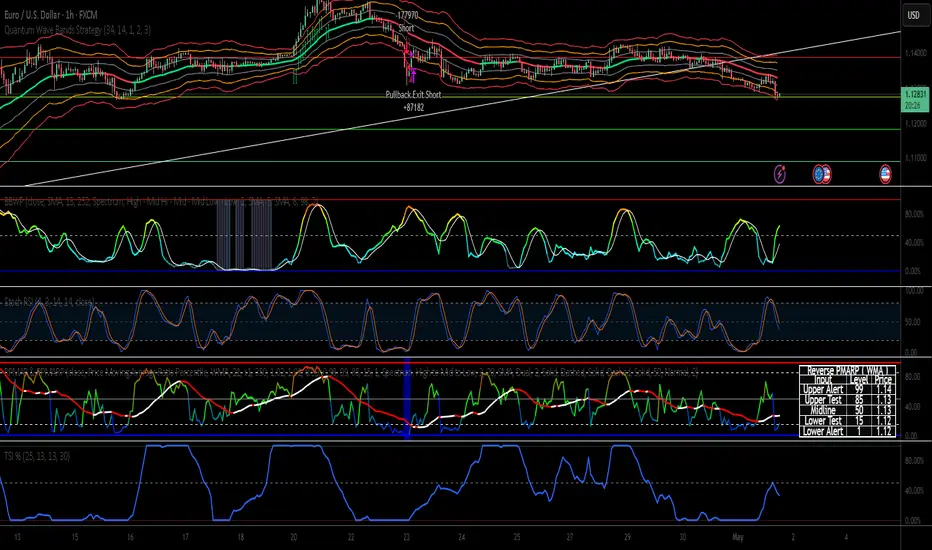
HL2 Moving Average with BandsThis indicator is designed to assist traders in identifying potential trade entries and exits for S&P 500 (ES) and Nasdaq-100 (NQ) futures. It calculates a Simple Moving Average (SMA) based on the HL2 value (average of high and low prices) of the current candle over a user-defined lookback period (default: 200 periods). The indicator plots this SMA as a blue line, providing a smoothed reference for price trends.
Additionally, it includes upper and lower bands calculated as a percentage (default: 0.5%) above and below the SMA, plotted as green and red lines, respectively. These bands act as dynamic thresholds to identify overbought or oversold conditions. The indicator generates trade signals based on price action relative to these bands:
Long Entry: A green upward triangle is plotted below the candle when the close crosses above the upper band, signaling a potential buy.
Close Long: A red square is plotted above the candle when the close crosses back below the upper band, indicating an exit for the long position.
Short Entry: A red downward triangle is plotted above the candle when the close crosses below the lower band, signaling a potential sell.
Close Short: A green square is plotted below the candle when the close crosses back above the lower band, indicating an exit for the short position.
The script is customizable, allowing users to adjust the SMA length and band percentage to suit their trading style or market conditions. It is plotted as an overlay on the price chart for easy integration with other technical analysis tools.
Recommended Time Frame and Settings for Trading S&P 500 and Nasdaq-100 Futures
Based on research and market dynamics for S&P 500 (ES) and Nasdaq-100 (NQ) futures, the 5-minute chart is recommended as the optimal time frame for day trading with this indicator. This time frame strikes a balance between capturing intraday trends and filtering out excessive noise, which is critical for futures trading due to their high volatility and leverage. The 5-minute chart aligns well with periods of high liquidity and volatility, such as the U.S. market open (9:30 AM–11:00 AM EST) and the afternoon session (2:00 PM–4:00 PM EST), when institutional traders are most active.
Why 5-minute? It allows traders to react to short-term price movements while avoiding the rapid fluctuations of 1-minute charts, which can be prone to false signals in choppy markets. It also provides enough data points to make the SMA and bands meaningful without the lag associated with longer time frames like 15-minute or hourly charts.
Recommended Settings
SMA Length: Set to 200 periods. This longer lookback period smooths the HL2 data, reducing noise and providing a reliable trend reference for the 5-minute chart. A 200-period SMA helps identify significant trend shifts without being overly sensitive to minor price fluctuations.
Band Percentage: 0.5% is more suitable for the volatility of ES and NQ futures on a 5-minute chart, as it generates fewer but higher-probability signals. Wider bands (e.g., 1%) may miss short-term opportunities, while narrower bands (e.g., 0.1%) may produce excessive false signals.
Trading Session Recommendations
Futures markets for ES and NQ are open nearly 24 hours (Sunday 6:00 PM EST to Friday 5:00 PM EST, with a daily break from 4:00 PM–5:00 PM EST), but not all hours are equally optimal due to varying liquidity and volatility. The best times to trade with this indicator are:
U.S. Market Open (9:30 AM–11:00 AM EST): This period is characterized by high volume and volatility, driven by the opening of U.S. equity markets and economic data releases (e.g., 8:30 AM EST reports like CPI or GDP). The indicator’s signals are more reliable during this window due to strong order flow and price momentum.
Afternoon Session (2:00 PM–4:00 PM EST): After the lunchtime lull, volume picks up as institutional traders return, and news or FOMC announcements often drive price action. The indicator can capture breakout moves as prices test the upper or lower bands.
Pre-Market (7:30 AM–9:30 AM EST): For traders comfortable with lower liquidity, this period can offer opportunities, especially around 8:30 AM EST economic releases. However, use tighter risk management due to wider spreads and potential volatility spikes.
Additional Tips
Avoid Low-Volume Periods: Steer clear of trading during low-liquidity hours, such as the overnight session (11:00 PM–3:00 AM EST), when spreads widen and price movements can be erratic, leading to false signals from the indicator.
Combine with Other Tools: Enhance the indicator’s effectiveness by pairing it with support/resistance levels, Fibonacci retracements, or volume analysis to confirm signals. For example, a long entry signal above the upper band is stronger if it coincides with a breakout above a key resistance level.
Risk Management: Given the leverage in futures (e.g., Micro E-mini contracts require ~$1,200 margin for ES), use tight stop-losses (e.g., below the lower band for longs or above the upper band for shorts) to manage risk. Aim for a risk-reward ratio of at least 1:2.
Test Settings: Backtest the indicator on a demo account to optimize the SMA length and band percentage for your specific trading style and risk tolerance. Micro E-mini contracts (MES for S&P 500, MNQ for Nasdaq-100) are ideal for testing due to their lower capital requirements.
Why These Settings and Time Frame?
The 5-minute chart with a 200-period SMA and 0.5% bands is tailored for the volatility and liquidity of ES and NQ futures during peak trading hours. The longer SMA period ensures the indicator captures meaningful trends, while the 0.5% bands are tight enough to signal actionable breakouts but wide enough to avoid excessive whipsaws. Trading during high-volume sessions maximizes the likelihood of valid signals, as institutional participation drives clearer price action.
By focusing on these settings and time frames, traders can leverage the indicator to capitalize on the dynamic price movements of S&P 500 and Nasdaq-100 futures while managing the inherent risks of these markets.