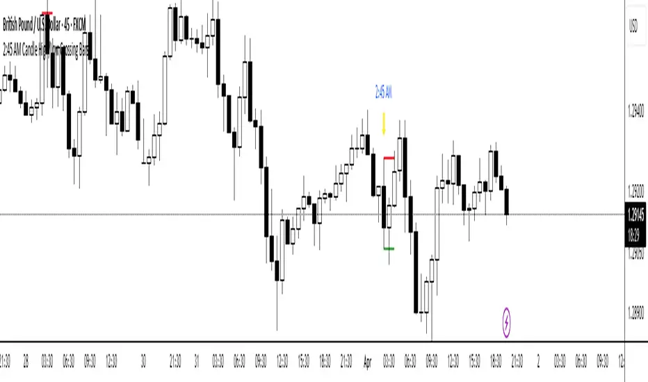
2:45 AM Candle High/Low Crossing Bars2:45 AM Candle High/Low Crossing Bars is an indicator that focuses on the trading view 2:45am NY TIME high and low indicating green for buy and red bars for sell, with the 2:45am new york time highlight/ If the next candle sweeps the low we buy while if it sweeps the high we sell, all time zoon must be the new York UTC time.
Cari dalam skrip untuk "沪深主板45度上升的股票"
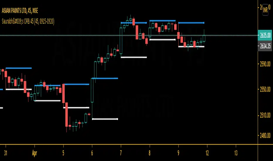
Saurabh's ORB 45This is indicator is all about opening range breakout on 45 mins charts.
|
|
|
|
|
which can be useful to day trader as a breakout strategy following the trend. Useful in 45 mins charts. Also, you may change the time frame from settings according to your likes.
Give thumbs up if you like it.
Opening Range Breakout (9:30 - 9:45 EST)Here's a Pine Script (v5) for TradingView that plots the Opening Range Breakout (ORB) lines from 9:30 AM to 9:45 AM EST on a 15-minute chart.
It draws a green line at the high of the opening range and a red line at the low, both extending through the rest of the day.

RSI Chart Bars 8 55 45Dear Traders
This RSI 8 period made for perfect entry for Long and Short for Intraday/Scalping in any time frame, when RSI 8 crossed above 55 the Candle charged to White then you can go for Long/Buy and when crossed below 45 the Candle changed to Yellow so you can go for Short/Sell, it working in any time frame.
Thanks & Regards
Nesan
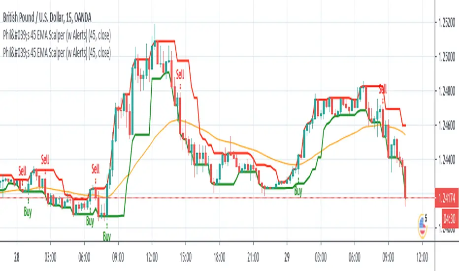
Phil's 45 EMA Scalper - Buy / Sell with Alertsgives buy / sell alert when candle closes above or below 45 EMA respectively.
EMA 9/45/90/180Easy script:
*4 EMAs : 9/45/90/180. You can change it if you want.
*Color change on crossover with close: Gives u an idea of the trend and mobile resistance/supports.
Let me know any suggestion!
Thx, bye.

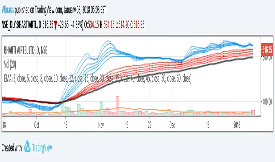
Guppy MMA 3, 5, 8, 10, 12, 15 and 30, 35, 40, 45, 50, 60Guppy Multiple Moving Average
Short Term EMA 3, 5, 8, 10, 12, 15
Long Term EMA 30, 35, 40, 45, 50, 60
Use for SFTS Class
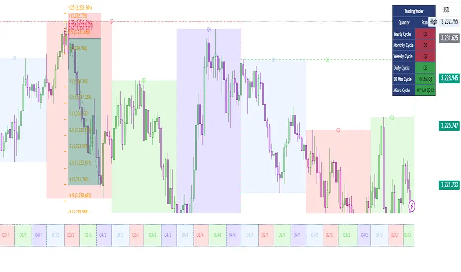
Quarterly Cycle Theory with DST time AdjustedThe Quarterly Theory removes ambiguity, as it gives specific time-based reference points to look for when entering trades. Before being able to apply this theory to trading, one must first understand that time is fractal:
Yearly Quarters = 4 quarters of three months each.
Monthly Quarters = 4 quarters of one week each.
Weekly Quarters = 4 quarters of one day each (Monday - Thursday). Friday has its own specific function.
Daily Quarters = 4 quarters of 6 hours each = 4 trading sessions of a trading day.
Sessions Quarters = 4 quarters of 90 minutes each.
90 Minute Quarters = 4 quarters of 22.5 minutes each.
Yearly Cycle: Analogously to financial quarters, the year is divided in four sections of three months each:
Q1 - January, February, March.
Q2 - April, May, June (True Open, April Open).
Q3 - July, August, September.
Q4 - October, November, December.
S&P 500 E-mini Futures (daily candles) — Monthly Cycle.
Monthly Cycle: Considering that we have four weeks in a month, we start the cycle on the first month’s Monday (regardless of the calendar Day):
Q1 - Week 1: first Monday of the month.
Q2 - Week 2: second Monday of the month (True Open, Daily Candle Open Price).
Q3 - Week 3: third Monday of the month.
Q4 - Week 4: fourth Monday of the month.
S&P 500 E-mini Futures (4 hour candles) — Weekly Cycle.
Weekly Cycle: Daye determined that although the trading week is composed by 5 trading days, we should ignore Friday, and the small portion of Sunday’s price action:
Q1 - Monday.
Q2 - Tuesday (True Open, Daily Candle Open Price).
Q3 - Wednesday.
Q4 - Thursday.
S&P 500 E-mini Futures (1 hour candles) — Daily Cycle.
Daily Cycle: The Day can be broken down into 6 hour quarters. These times roughly define the sessions of the trading day, reinforcing the theory’s validity:
Q1 - 18:00 - 00:00 Asia.
Q2 - 00:00 - 06:00 London (True Open).
Q3 - 06:00 - 12:00 NY AM.
Q4 - 12:00 - 18:00 NY PM.
S&P 500 E-mini Futures (15 minute candles) — 6 Hour Cycle.
6 Hour Quarters or 90 Minute Cycle / Sessions divided into four sections of 90 minutes each (EST/EDT):
Asian Session
Q1 - 18:00 - 19:30
Q2 - 19:30 - 21:00 (True Open)
Q3 - 21:00 - 22:30
Q4 - 22:30 - 00:00
London Session
Q1 - 00:00 - 01:30
Q2 - 01:30 - 03:00 (True Open)
Q3 - 03:00 - 04:30
Q4 - 04:30 - 06:00
NY AM Session
Q1 - 06:00 - 07:30
Q2 - 07:30 - 09:00 (True Open)
Q3 - 09:00 - 10:30
Q4 - 10:30 - 12:00
NY PM Session
Q1 - 12:00 - 13:30
Q2 - 13:30 - 15:00 (True Open)
Q3 - 15:00 - 16:30
Q4 - 16:30 - 18:00
S&P 500 E-mini Futures (5 minute candles) — 90 Minute Cycle.
Micro Cycles: Dividing the 90 Minute Cycle yields 22.5 Minute Quarters, also known as Micro Sessions or Micro Quarters:
Asian Session
Q1/1 18:00:00 - 18:22:30
Q2 18:22:30 - 18:45:00
Q3 18:45:00 - 19:07:30
Q4 19:07:30 - 19:30:00
Q2/1 19:30:00 - 19:52:30 (True Session Open)
Q2/2 19:52:30 - 20:15:00
Q2/3 20:15:00 - 20:37:30
Q2/4 20:37:30 - 21:00:00
Q3/1 21:00:00 - 21:23:30
etc. 21:23:30 - 21:45:00
London Session
00:00:00 - 00:22:30 (True Daily Open)
00:22:30 - 00:45:00
00:45:00 - 01:07:30
01:07:30 - 01:30:00
01:30:00 - 01:52:30 (True Session Open)
01:52:30 - 02:15:00
02:15:00 - 02:37:30
02:37:30 - 03:00:00
03:00:00 - 03:22:30
03:22:30 - 03:45:00
03:45:00 - 04:07:30
04:07:30 - 04:30:00
04:30:00 - 04:52:30
04:52:30 - 05:15:00
05:15:00 - 05:37:30
05:37:30 - 06:00:00
New York AM Session
06:00:00 - 06:22:30
06:22:30 - 06:45:00
06:45:00 - 07:07:30
07:07:30 - 07:30:00
07:30:00 - 07:52:30 (True Session Open)
07:52:30 - 08:15:00
08:15:00 - 08:37:30
08:37:30 - 09:00:00
09:00:00 - 09:22:30
09:22:30 - 09:45:00
09:45:00 - 10:07:30
10:07:30 - 10:30:00
10:30:00 - 10:52:30
10:52:30 - 11:15:00
11:15:00 - 11:37:30
11:37:30 - 12:00:00
New York PM Session
12:00:00 - 12:22:30
12:22:30 - 12:45:00
12:45:00 - 13:07:30
13:07:30 - 13:30:00
13:30:00 - 13:52:30 (True Session Open)
13:52:30 - 14:15:00
14:15:00 - 14:37:30
14:37:30 - 15:00:00
15:00:00 - 15:22:30
15:22:30 - 15:45:00
15:45:00 - 15:37:30
15:37:30 - 16:00:00
16:00:00 - 16:22:30
16:22:30 - 16:45:00
16:45:00 - 17:07:30
17:07:30 - 18:00:00
S&P 500 E-mini Futures (30 second candles) — 22.5 Minute Cycle.
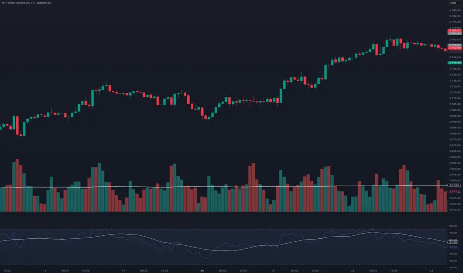
Relative Strength Index With Range ZoneRSI (Relative Strength Index) with 45-55 Range Zone
1. Introduction and Historical Background
The Relative Strength Index (RSI) is a momentum indicator developed in 1978 by J. Welles Wilder Jr. It measures the speed and magnitude of price changes to assess overbought and oversold conditions of an asset. This widely used oscillator ranges between 0 and 100.
Historically, the RSI was mainly used to detect trend reversals by identifying extreme levels: above 70 (overbought) and below 30 (oversold). However, its application has evolved, and new approaches refine its interpretation, such as adding a 45-55 neutral zone to identify consolidation (range) periods.
2. RSI Calculation
The RSI is calculated using the following formula:
RSI=100−(1001+RS)RSI=100−(1+RS100)
Where:
RS=Average gain over N periodsAverage loss over N periodsRS=Average loss over N periodsAverage gain over N periods
• RS (Relative Strength) is the ratio between the average gains and the average losses over N periods (typically 14 periods).
• Gains and losses are calculated based on daily price variations.
Example calculation with a 14-day period:
1. Compute daily gains and losses.
2. Take an exponential or simple moving average of these values over 14 days.
3. Apply the formula to get the RSI value.
3. Classic RSI Usage
The RSI is typically interpreted as follows:
• RSI > 70: Overbought → Possible correction or bearish reversal.
• RSI < 30: Oversold → Possible rebound or bullish reversal.
• RSI between 50 and 70: Bullish momentum.
• RSI between 30 and 50: Bearish momentum.
4. Adding the 45-55 Zone to Identify Range Phases
Adding a neutral zone between 45 and 55 helps identify consolidation periods, when price moves sideways without a strong trend.
• RSI between 45 and 55: The market is in a range, meaning neither buyers nor sellers dominate.
• RSI breaking out of this zone:
o Above 55: Indicates the start of a bullish trend.
o Below 45: Indicates the start of a bearish trend.
This zone is particularly useful for:
• Avoiding false signals by waiting for trend confirmation.
• Identifying ranging markets, favoring range trading strategies (buying at support, selling at resistance).
• Filtering trend-based entries, waiting for the RSI to exit the 45-55 zone.
5. Trading Strategies Using RSI with the 45-55 Range Zone
1. Range Trading:
• When the RSI oscillates between 45 and 55, it signals a lack of strong trend.
• Strategy:
o Identify a support and resistance level.
o Buy near support when the RSI touches 45.
o Sell near resistance when the RSI touches 55.
2. Breakout Trading:
• If the RSI exits the 45-55 zone:
o Above 55 → Buy (start of a bullish trend).
o Below 45 → Sell (start of a bearish trend).
• This breakout can be used as a confirmed entry signal.
3. Confirmation with Divergences:
• A bullish divergence (price making lower lows while RSI makes higher lows) is more relevant if the RSI moves above 55.
• A bearish divergence (price making higher highs while RSI makes lower highs) is stronger if the RSI drops below 45.
6. Conclusion
The RSI is a powerful tool for analyzing price momentum. Adding a 45-55 zone enhances its usage by clearly distinguishing:
• Consolidation phases (range markets).
• Trend beginnings when RSI breaks out of this range.
This approach improves RSI reliability by filtering out false signals and allowing traders to adapt their strategy based on market conditions.
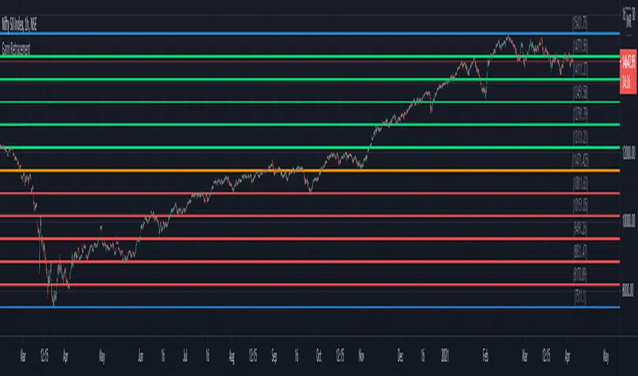
Gann RetracementThe indicator is based on W. D. Gann's method of retracement studies. Gann looked at stock retracement action in terms of Halves (1/2), Thirds (1/3, 2/3), Fifths (1/5, 2/5, 3/5, and 4/5) and more importantly the Eighths (1/8, 2/8, 3/8, 4/8, 5/8, 6/8, and 7/8). Needless to say, {2, 3, 5, 8} are the only Fibonacci numbers between 1 to 10. These ratios can easily be visualized in the form of division of a Circle as follows :
Divide the circle in 12 equal parts of 30 degree each to produce the Thirds :
30 x 4 = 120 is 1/3 of 360
30 x 8 = 240 is 2/3 of 360
The 30 degree retracement captures fundamental geometric shapes like a regular Triangle (120-240-360), a Square (90-180-270-360), and a regular Hexagon (60-120-180-240-300-360) inscribed inside of the circle.
Now, divide the circle in 10 equal parts of 36 degree each to produce the Fifths :
36 x 2 = 72 is 1/5 of 360
36 x 4 = 144 is 2/5 of 360
36 x 6 = 216 is 3/5 of 360
36 x 8 = 288 is 4/5 of 360
where, (72-144-216-288-360) is a regular Pentagon.
Finally, divide the circle in 8 equal parts of 45 degree each to produce the Eighths :
45 x 1 = 45 is 1/8 of 360
45 x 2 = 90 is 2/8 of 360
45 x 3 = 135 is 3/8 of 360
45 x 4 = 180 is 4/8 of 360
45 x 5 = 225 is 5/8 of 360
45 x 6 = 270 is 6/8 of 360
45 x 7 = 315 is 7/8 of 360
where, (45-90-135-180-225-270-315-360) is a regular Octagon.
How to Use this indicator ?
The indicator generates Gann retracement levels between any two significant price points, such as a high and a low.
Input :
Swing High (significant high price point, such as a top)
Swing Low (significant low price point, such as a bottom)
Degree (degree of retracement)
Output :
Gann retracement levels (color coded as follows) :
Swing High and Swing Low (BLUE)
50% retracement (ORANGE)
Retracements between Swing Low and 50% level (RED)
Retracements between 50% level and Swing High (LIME)
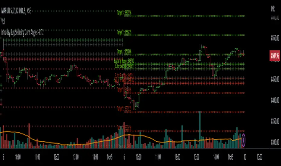
Intraday Buy/Sell using Gann Angles - RiTzIntraday Buy/Sell Levels using Gann Angles based on Todays Open/previous Day High/Low/Close prices
How to use this :
The Buy/Sell levels will be calculated on 1 of 4 things (you can choose any one which you prefer)
1. Todays Open price
2. Previous Day High
3. Previous Day Low
4. Previous Day Close
The Buy/Sell levels will be displayed in these ways
1. In a Table
2. on the Chart
You can turn them on/off according to your preference!
I can't seem to find the original documentation or a link to it.
i have it's excel file, in which we have to enter following data :
1. Todays Open price
2. Previous Day High
3. Previous Day Low
4. Previous Day Close
and the buy/sell levels are calculated by using the above data in following manner :
Based On Today's Opening Price
(lets call it TDO)
Degree's````````````````` Degree Factor```````````````````````` Buy````````````````````````` Sell
11.25```````````````````` =degree/180=11.25/180=0.0625````````` =(sqrt(TDO)-0.0625)^2``````` =(sqrt(TDO)+0.0625)^2````` SL
22.5````````````````````` =degree/180=22.5/180=0.125``````````` =(sqrt(TDO)+0.125)^2```````` =(sqrt(TDO)-0.125)^2`````` Buy/Sell At
45``````````````````````` =degree/180=45/180=0.25`````````````` =(sqrt(TDO)+0.25)^2````````` =(sqrt(TDO)-0.25)^2``````` Target-1
90``````````````````````` =degree/180=90/180=0.5``````````````` =(sqrt(TDO)+0.5)^2`````````` =(sqrt(TDO)-0.5)^2```````` Target-2
135`````````````````````` =degree/180=135/180=0.75````````````` =(sqrt(TDO)+0.75)^2````````` =(sqrt(TDO)-0.75)^2``````` Target-3
180`````````````````````` =degree/180=180/180=1```````````````` =(sqrt(TDO)+1)^2```````````` =(sqrt(TDO)-1)^2`````````` Target-4
225`````````````````````` =degree/180=225/180=1.25````````````` =(sqrt(TDO)+1.25)^2````````` =(sqrt(TDO)-1.25)^2``````` Target-5
270`````````````````````` =degree/180=270/180=1.5`````````````` =(sqrt(TDO)+1.5)^2`````````` =(sqrt(TDO)-1.5)^2```````` Target-6
315`````````````````````` =degree/180=315/180=1.75````````````` =(sqrt(TDO)+1.75)^2````````` =(sqrt(TDO)-1.75)^2``````` Target-7
360`````````````````````` =degree/180=360/180=2```````````````` =(sqrt(TDO)+2)^2```````````` =(sqrt(TDO)-2)^2`````````` Target-8
sqrt = square root
TDO = Today's Opening Price
PDH = Previous Days High
PDL = Previous Days Low
PDC = Previous Days Close
Based On Previous Days High Price
(lets call it PDH)
Degree's````````````````` Degree Factor```````````````````````` Buy````````````````````````` Sell
11.25```````````````````` =degree/180=11.25/180=0.0625````````` =(sqrt(PDH)-0.0625)^2``````` =(sqrt(PDH)+0.0625)^2````` SL
22.5````````````````````` =degree/180=22.5/180=0.125``````````` =(sqrt(PDH)+0.125)^2```````` =(sqrt(PDH)-0.125)^2`````` Buy/Sell At
45``````````````````````` =degree/180=45/180=0.25`````````````` =(sqrt(PDH)+0.25)^2````````` =(sqrt(PDH)-0.25)^2``````` Target-1
90``````````````````````` =degree/180=90/180=0.5``````````````` =(sqrt(PDH)+0.5)^2`````````` =(sqrt(PDH)-0.5)^2```````` Target-2
135`````````````````````` =degree/180=135/180=0.75````````````` =(sqrt(PDH)+0.75)^2````````` =(sqrt(PDH)-0.75)^2``````` Target-3
180`````````````````````` =degree/180=180/180=1```````````````` =(sqrt(PDH)+1)^2```````````` =(sqrt(PDH)-1)^2`````````` Target-4
225`````````````````````` =degree/180=225/180=1.25````````````` =(sqrt(PDH)+1.25)^2````````` =(sqrt(PDH)-1.25)^2``````` Target-5
270`````````````````````` =degree/180=270/180=1.5`````````````` =(sqrt(PDH)+1.5)^2`````````` =(sqrt(PDH)-1.5)^2```````` Target-6
315`````````````````````` =degree/180=315/180=1.75````````````` =(sqrt(PDH)+1.75)^2````````` =(sqrt(PDH)-1.75)^2``````` Target-7
360`````````````````````` =degree/180=360/180=2```````````````` =(sqrt(PDH)+2)^2```````````` =(sqrt(PDH)-2)^2`````````` Target-8
Based On Previous Days Low Price
(lets call it PDL)
Degree's````````````````` Degree Factor```````````````````````` Buy````````````````````````` Sell
11.25```````````````````` =degree/180=11.25/180=0.0625````````` =(sqrt(PDL)-0.0625)^2``````` =(sqrt(PDL)+0.0625)^2````` SL
22.5````````````````````` =degree/180=22.5/180=0.125``````````` =(sqrt(PDL)+0.125)^2```````` =(sqrt(PDL)-0.125)^2`````` Buy/Sell At
45``````````````````````` =degree/180=45/180=0.25`````````````` =(sqrt(PDL)+0.25)^2````````` =(sqrt(PDL)-0.25)^2``````` Target-1
90``````````````````````` =degree/180=90/180=0.5``````````````` =(sqrt(PDL)+0.5)^2`````````` =(sqrt(PDL)-0.5)^2```````` Target-2
135`````````````````````` =degree/180=135/180=0.75````````````` =(sqrt(PDL)+0.75)^2````````` =(sqrt(PDL)-0.75)^2``````` Target-3
180`````````````````````` =degree/180=180/180=1```````````````` =(sqrt(PDL)+1)^2```````````` =(sqrt(PDL)-1)^2`````````` Target-4
225`````````````````````` =degree/180=225/180=1.25````````````` =(sqrt(PDL)+1.25)^2````````` =(sqrt(PDL)-1.25)^2``````` Target-5
270`````````````````````` =degree/180=270/180=1.5`````````````` =(sqrt(PDL)+1.5)^2`````````` =(sqrt(PDL)-1.5)^2```````` Target-6
315`````````````````````` =degree/180=315/180=1.75````````````` =(sqrt(PDL)+1.75)^2````````` =(sqrt(PDL)-1.75)^2``````` Target-7
360`````````````````````` =degree/180=360/180=2```````````````` =(sqrt(PDL)+2)^2```````````` =(sqrt(PDL)-2)^2`````````` Target-8
Based On Previous Days Close Price
(lets call it PDC)
Degree's````````````````` Degree Factor```````````````````````` Buy````````````````````````` Sell
11.25```````````````````` =degree/180=11.25/180=0.0625````````` =(sqrt(PDC)-0.0625)^2``````` =(sqrt(PDC)+0.0625)^2````` SL
22.5````````````````````` =degree/180=22.5/180=0.125``````````` =(sqrt(PDC)+0.125)^2```````` =(sqrt(PDC)-0.125)^2`````` Buy/Sell At
45``````````````````````` =degree/180=45/180=0.25`````````````` =(sqrt(PDC)+0.25)^2````````` =(sqrt(PDC)-0.25)^2``````` Target-1
90``````````````````````` =degree/180=90/180=0.5``````````````` =(sqrt(PDC)+0.5)^2`````````` =(sqrt(PDC)-0.5)^2```````` Target-2
135`````````````````````` =degree/180=135/180=0.75````````````` =(sqrt(PDC)+0.75)^2````````` =(sqrt(PDC)-0.75)^2``````` Target-3
180`````````````````````` =degree/180=180/180=1```````````````` =(sqrt(PDC)+1)^2```````````` =(sqrt(PDC)-1)^2`````````` Target-4
225`````````````````````` =degree/180=225/180=1.25````````````` =(sqrt(PDC)+1.25)^2````````` =(sqrt(PDC)-1.25)^2``````` Target-5
270`````````````````````` =degree/180=270/180=1.5`````````````` =(sqrt(PDC)+1.5)^2`````````` =(sqrt(PDC)-1.5)^2```````` Target-6
315`````````````````````` =degree/180=315/180=1.75````````````` =(sqrt(PDC)+1.75)^2````````` =(sqrt(PDC)-1.75)^2``````` Target-7
360`````````````````````` =degree/180=360/180=2```````````````` =(sqrt(PDC)+2)^2```````````` =(sqrt(PDC)-2)^2`````````` Target-8
example based On Today's Opening Price = 4339
Degree's```````` Degree Factor```````` Buy`````````` Sell
11.25``````````` 0.0625``````````````` 4330.77`````` 4347.24```````` SL
22.5```````````` 0.125```````````````` 4355.48`````` 4322.55```````` Buy/Sell At
45`````````````` 0.25````````````````` 4372.00`````` 4306.13```````` Target-1
90`````````````` 0.5`````````````````` 4405.12`````` 4273.38```````` Target-2
135````````````` 0.75````````````````` 4438.37`````` 4240.76```````` Target-3
180````````````` 1```````````````````` 4471.74`````` 4208.26```````` Target-4
225````````````` 1.25````````````````` 4505.24`````` 4175.88```````` Target-5
270````````````` 1.5`````````````````` 4538.86`````` 4143.64```````` Target-6
315````````````` 1.75````````````````` 4572.61`````` 4111.51```````` Target-7
360````````````` 2```````````````````` 4606.48`````` 4079.52```````` Target-8
Note : ignore the '`' , inserted them to fill up the spaces , it was looking very weird!, tried to fix it as much as I can.
Note :- Please correct me if I'm wrong , as I've already mentioned I don't have it's original documentation.
if anyone can find it or already has it then please feel free to share it.
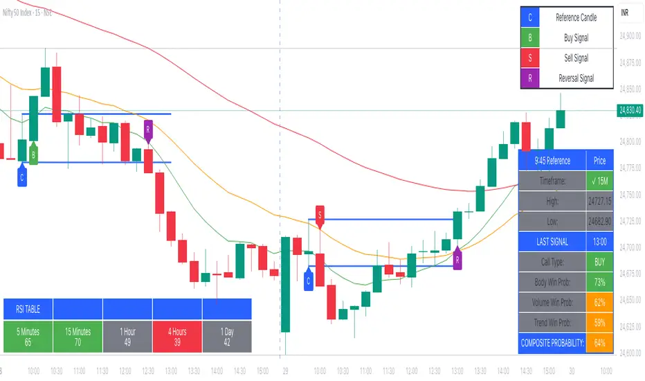
9:45am NIFTY TRADINGTime Frame: 15 Minutes | Reference Candle Time: 9:45 AM IST | Valid Trading Window: 3 Hours
📌 Introduction
This document outlines a structured trading strategy for NIFTY & BANKNIFTY Options based on a 15-minute timeframe with a 9:45 AM IST reference candle. The strategy incorporates technical indicators, probability analysis, and strict trading rules to optimize entries and exits.
📊 Core Features
1. Reference Time Trading System
9:45 AM IST Candle acts as the reference for the day.
All signals (Buy/Sell/Reversal) are generated based on price action relative to this candle.
The valid trading window is 3 hours after the reference candle.
2. Signal Generation Logic
Signal Condition
Buy (B) Price breaks above reference candle high with confirmation
Sell (S) Price breaks below reference candle low with confirmation
Reversal (R) Early trend reversal signal (requires strict confirmation)
3. Probability Analysis System
The strategy calculates Win Probability (%) using 4 components:
Component Weight Calculation
Body Win Probability 30% Based on candle body strength (body % of total range)
Volume Win Probability 30% Current volume vs. average volume strength
Trend Win Probability 40% EMA crossover + RSI momentum alignment
Composite Probability - Weighted average of all 3 components
Probability Color Coding:
🟢 Green (High Probability): ≥70%
🟠 Orange (Medium Probability): 50-69%
🔴 Red (Low Probability): <50%
4. Timeframe Enforcement
Strictly 15-minute charts only (no other timeframes allowed).
System auto-disables signals if the wrong timeframe is selected.
📈 Technical Analysis Components
1. EMA System (Trend Analysis)
Short EMA (9) – Fast trend indicator
Middle EMA (20) – Intermediate trend
Long EMA (50) – Long-term trend confirmation
Rules:
Buy Signal: Price > 9 EMA > 20 EMA > 50 EMA (Bullish trend)
Sell Signal: Price < 9 EMA < 20 EMA < 50 EMA (Bearish trend)
2. Multi-Timeframe RSI (Momentum)
5M, 15M, 1H, 4H, Daily RSI values are compared for divergence/confluence.
Overbought (≥70) / Oversold (≤30) conditions help in reversal signals.
3. Volume Analysis
Volume Strength (%) = (Current Volume / Avg. Volume) × 100
Strong Volume (>120% Avg.) confirms breakout/breakdown.
4. Body Percentage (Candle Strength)
Body % = (Close - Open) / (High - Low) × 100
Strong Bullish Candle: Body > 60%
Strong Bearish Candle: Body < 40%
📊 Visual Elements
1. Information Tables
Reference Data Table (9:45 AM Candle High/Low/Close)
RSI Values Table (5M, 15M, 1H, 4H, Daily)
Signal Legend (Buy/Sell/Reversal indicators)
2. Chart Overlays
Reference Lines (9:45 AM High & Low)
EMA Lines (9, 20, 50)
Signal Labels (B, S, R)
3. Color Coding
High Probability (Green)
Medium Probability (Orange)
Low Probability (Red)
⚠️ Important Usage Guidelines
✅ Best Practices:
Trade only within the 3-hour window (9:45 AM - 12:45 PM IST).
Wait for confirmation (closing above/below reference candle).
Use probability score to filter high-confidence trades.
❌ Avoid:
Trading outside the 15-minute timeframe.
Ignoring volume & RSI divergence.
Overtrading – Stick to 1-2 high-probability setups per day.
🎯 Conclusion
This NIFTY Trading Strategy is optimized for 15-minute charts with a 9:45 AM IST reference candle. It combines EMA trends, RSI momentum, volume analysis, and probability scoring to generate high-confidence signals.
🚀 Key Takeaways:
✔ Reference candle defines the day’s bias.
✔ Probability system filters best trades.
✔ Strict 15M timeframe ensures consistency.
Happy Trading! 📈💰
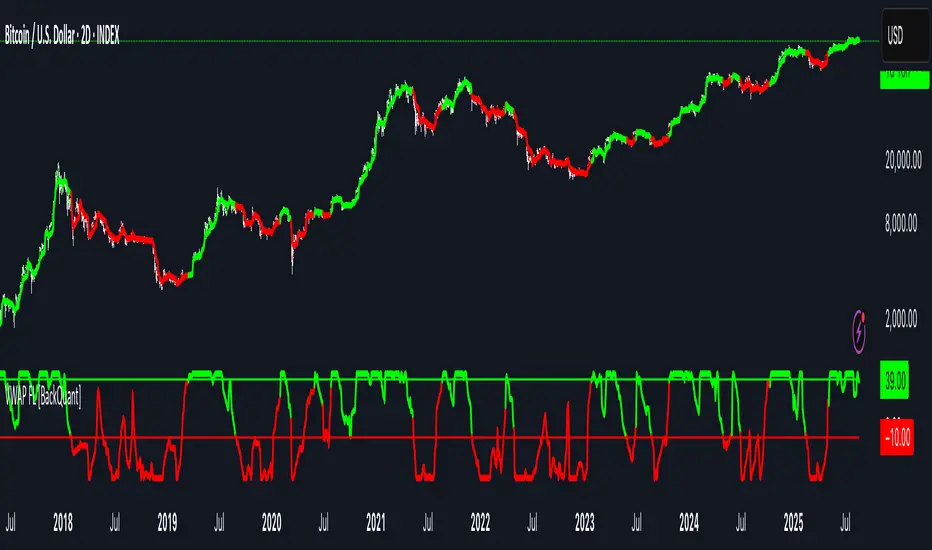
VWAP For Loop [BackQuant]VWAP For Loop
What this tool does—in one sentence
A volume-weighted trend gauge that anchors VWAP to a calendar period (day/week/month/quarter/year) and then scores the persistence of that VWAP trend with a simple for-loop “breadth” count; the result is a clean, threshold-driven oscillator plus an optional VWAP overlay and alerts.
Plain-English overview
Instead of judging raw price alone, this indicator focuses on anchored VWAP —the market’s average price paid during your chosen institutional period. It then asks a simple question across a configurable set of lookback steps: “Is the current anchored VWAP higher than it was i bars ago—or lower?” Each “yes” adds +1, each “no” adds −1. Summing those answers creates a score that reflects how consistently the volume-weighted trend has been rising or falling. Extreme positive scores imply persistent, broad strength; deeply negative scores imply persistent weakness. Crossing predefined thresholds produces objective long/short events and color-coded context.
Under the hood
• Anchoring — VWAP using hlc3 × volume resets exactly when the selected period rolls:
Day → session change, Week → new week, Month → new month, Quarter/Year → calendar quarter/year.
• For-loop scoring — For lag steps i = , compare today’s VWAP to VWAP .
– If VWAP > VWAP , add +1.
– Else, add −1.
The final score ∈ , where N = (end − start + 1). With defaults (1→45), N = 45.
• Signal logic (stateful)
– Long when score > upper (e.g., > 40 with N = 45 → VWAP higher than ~89% of checked lags).
– Short on crossunder of lower (e.g., dropping below −10).
– A compact state variable ( out ) holds the current regime: +1 (long), −1 (short), otherwise unchanged. This “stickiness” avoids constant flipping between bars without sufficient evidence.
Why VWAP + a breadth score?
• VWAP aggregates both price and volume—where participants actually traded.
• The breadth-style count rewards consistency of the anchored trend, not one-off spikes.
• Thresholds give you binary structure when you need it (alerts, automation), without complex math.
What you’ll see on the chart
• Sub-pane oscillator — The for-loop score line, colored by regime (long/short/neutral).
• Main-pane VWAP (optional) — Even though the indicator runs off-chart, the anchored VWAP can be overlaid on price (toggle visibility and whether it inherits trend colors).
• Threshold guides — Horizontal lines for the long/short bands (toggle).
• Cosmetics — Optional candle painting and background shading by regime; adjustable line width and colors.
Input map (quick reference)
• VWAP Anchor Period — Day, Week, Month, Quarter, Year.
• Calculation Start/End — The for-loop lag window . With 1→45, you evaluate 45 comparisons.
• Long/Short Thresholds — Default upper=40, lower=−10 (asymmetric by design; see below).
• UI/Style — Show thresholds, paint candles, background color, line width, VWAP visibility and coloring, custom long/short colors.
Interpreting the score
• Near +N — Current anchored VWAP is above most historical VWAP checkpoints in the window → entrenched strength.
• Near −N — Current anchored VWAP is below most checkpoints → entrenched weakness.
• Between — Mixed, choppy, or transitioning regimes; use thresholds to avoid reacting to noise.
Why the asymmetric default thresholds?
• Long = score > upper (40) — Demands unusually broad upside persistence before declaring “long regime.”
• Short = crossunder lower (−10) — Triggers only on downward momentum events (a fresh breach), not merely being below −10. This combination tends to:
– Capture sustained uptrends only when they’re very strong.
– Flag downside turns as they occur, rather than waiting for an extreme negative breadth.
Tuning guide
Choose an anchor that matches your horizon
– Intraday scalps : Day anchor on intraday charts.
– Swing/position : Month or Quarter anchor on 1h/4h/D charts to capture institutional cycles.
Pick the for-loop window
– Larger N (bigger end) = stronger evidence requirement, smoother oscillator.
– Smaller N = faster, more reactive score.
Set achievable thresholds
– Ensure upper ≤ N and lower ≥ −N ; if N=30, an upper of 40 can never trigger.
– Symmetric setups (e.g., +20/−20) are fine if you want balanced behavior.
Match visuals to intent
– Enabling VWAP coloring lets you see regime directly on price.
– Background shading is useful for discretionary reading; turn it off for cleaner automation displays.
Playbook examples
• Trend confirmation with disciplined entries — On Month anchor, N=45, upper=38–42: when the long regime engages, use pullbacks toward anchored VWAP on the main pane for entries, with stops just beyond VWAP or a recent swing.
• Downside transition detection — Keep lower around −8…−12 and watch for crossunders; combine with price losing anchored VWAP to validate risk-off.
• Intraday bias filter — Day anchor on a 5–15m chart, N=20–30, upper ~ 16–20, lower ~ −6…−10. Only take longs while score is positive and above a midline you define (e.g., 0), and shorts only after a genuine crossunder.
Behavior around resets (important)
Anchored VWAP is hard-reset each period. Immediately after a reset, the series can be young and comparisons to pre-reset values may span two periods. If you prefer within-period evaluation only, choose end small enough not to bridge typical period length on your timeframe, or accept that the breadth test intentionally spans regimes.
Alerts included
• VWAP FL Long — Fires when the long condition is true (score > upper and not in short).
• VWAP FL Short — Fires on crossunder of the lower threshold (event-driven).
Messages include {{ticker}} and {{interval}} placeholders for routing.
Strengths
• Simple, transparent math — Easy to reason about and validate.
• Volume-aware by construction — Decisions reference VWAP, not just price.
• Robust to single-bar noise — Needs many lags to agree before flipping state (by design, via thresholds and the stateful output).
Limitations & cautions
• Threshold feasibility — If N < upper or |lower| > N, signals will never trigger; always cross-check N.
• Path dependence — The state variable persists until a new event; if you want frequent re-evaluation, lower thresholds or reduce N.
• Regime changes — Calendar resets can produce early ambiguity; expect a few bars for the breadth to mature.
• VWAP sensitivity to volume spikes — Large prints can tilt VWAP abruptly; that behavior is intentional in VWAP-based logic.
Suggested starting profiles
• Intraday trend bias : Anchor=Day, N=25 (1→25), upper=18–20, lower=−8, paint candles ON.
• Swing bias : Anchor=Month, N=45 (1→45), upper=38–42, lower=−10, VWAP coloring ON, background OFF.
• Balanced reactivity : Anchor=Week, N=30 (1→30), upper=20–22, lower=−10…−12, symmetric if desired.
Implementation notes
• The indicator runs in a separate pane (oscillator), but VWAP itself is drawn on price using forced overlay so you can see interactions (touches, reclaim/loss).
• HLC3 is used for VWAP price; that’s a common choice to dampen wick noise while still reflecting intrabar range.
• For-loop cap is kept modest (≤50) for performance and clarity.
How to use this responsibly
Treat the oscillator as a bias and persistence meter . Combine it with your entry framework (structure breaks, liquidity zones, higher-timeframe context) and risk controls. The design emphasizes clarity over complexity—its edge is in how strictly it demands agreement before declaring a regime, not in predicting specific turns.
Summary
VWAP For Loop distills the question “How broadly is the anchored, volume-weighted trend advancing or retreating?” into a single, thresholded score you can read at a glance, alert on, and color through your chart. With careful anchoring and thresholds sized to your window length, it becomes a pragmatic bias filter for both systematic and discretionary workflows.
15-Minute ORB by @RhinoTradezOverview
Hey traders, ready to jump on the morning breakout train? The 15-Minute ORB by @RhinoTradez
is your go-to pal for rocking the Opening Range Breakout (ORB) scene, zeroing in on the first 15 minutes of the U.S. market day—9:30 to 9:45 AM Eastern Time. Picture this: sleek orange lines mark the high and low of that opening rush, but they only hang out during regular trading hours (9:30 AM-4:00 PM ET) and reset fresh each day—no old baggage here! Built in Pine Script v6 for that cutting-edge feel, it’s loaded with breakout signals and alerts to keep your trading game strong—ideal for SPY, QQQ, or any ticker you love.
Crafted by @RhinoTradez
to fuel your daily grind—let’s hit those breakouts running!
What It Does
The ORB strategy is all about that early market spark: the 9:30-9:45 AM range sets the battlefield, and breakouts signal the charge. Here’s the rundown:
Captures the Range : Snags the high and low from the 9:30-9:45 AM ET candle—U.S. market kickoff, locked in.
Daily Refresh : Wipes yesterday’s lines at 9:30 AM ET each day—today’s all that matters.
Regular Hours Focus : Orange lines shine from 9:45 AM to 4:00 PM ET, vanishing outside those hours.
Breakout Signals : Green triangles for upside breaks, red for downside, all within regular hours.
Alerts You : Chimes in with “Price broke above 15-min ORB High: 597” (or below the low) when the move hits.
It’s your morning breakout blueprint—simple, focused, and trader-ready.
Functionality Breakdown:
15-Minute ORB Snap:
Locks the high and low of the 9:30-9:45 AM ET candle on a 15-minute chart (EST/EDT auto-adjusted).
Resets daily at 9:30 AM ET—yesterday’s range is outta here.
Regular Hours Only:
Lines glow from 9:45 AM to 4:00 PM ET, keeping pre-market and after-hours clean.
Breakout Flags:
Marks price busting above the ORB high (green triangle below bar) or below the low (red triangle above), only during 9:30 AM-4:00 PM.
Alert Action:
Drops a custom alert with the breakout price (e.g., “Price broke below 15-min ORB Low: 594”)—stay in the know, hands-free.
Customization Options
Keep it chill with one slick tweak:
ORB Line Color : Starts at orange—vibrant and trader-cool! Flip it to blue, purple, or any shade you dig in the settings. Make it yours.
How to Use It
Pop It On: Add it to a 15-minute chart—SPY, QQQ, or your hot pick works like a dream.
Time It Right: Set your chart to “America/New_York” time (Chart Settings > Time Zone) to sync with 9:30 AM ET.
Choose Your Color: Dive into the indicator settings and pick your ORB line color—orange kicks it off, but you’re in charge.
Set Alerts: Right-click the indicator, add an alert with “Any alert() function call,” and catch breakouts live.
Ride the Wave: Green triangle? Upward vibe. Red? Downside alert. Mix with volume or candles for extra punch.
Pro Tips
15-Minute Only : Tailored for that 9:30-9:45 AM ET candle—other timeframes won’t sync up.
Daily Reset : Lines refresh at 9:30 AM ET—always today’s play.
Breakout Boost : High volume or RSI can seal the deal on those triangle signals.
No Clutter : Lines stick to 9:30 AM-4:00 PM ET—your chart stays tidy.
Brought to you by @RhinoTradez
in Pine Script v6, this ORB script’s your morning breakout wingman. Slap it on, pick a color, and let’s chase those moves together! Happy trading!

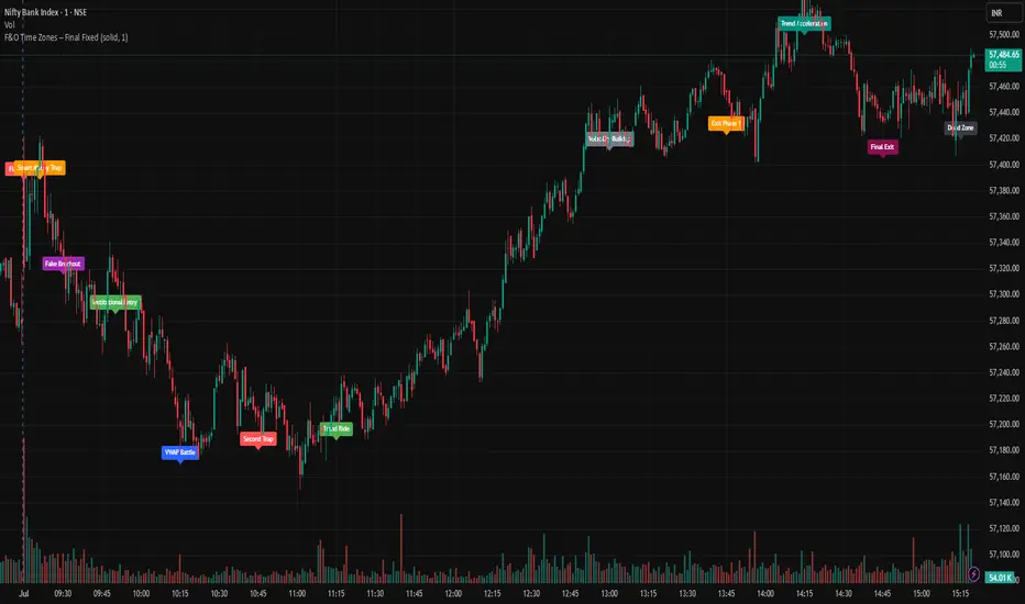
F&O Time Zones – Final Fixed📌 This indicator highlights high-probability intraday time zones used in Indian F&O (Futures & Options) strategies. Ideal for scalping, breakout setups, and trap avoidance.
🕒 Covered Time Zones:
• 9:15 – 9:21 AM → Flash Trades (first 1-minute volatility)
• 9:21 – 9:30 AM → Smart Money Trap (VWAP fakeouts)
• 9:30 – 9:50 AM → Fake Breakout Zone
• 9:50 – 10:15 AM → Institutional Entry Timing
• 10:15 – 10:45 AM → VWAP Range Scalps
• 10:45 – 11:15 AM → Second Trap Zone
• 11:15 – 1:00 PM → Trend Continuation Window
• 1:00 – 1:45 PM → Volatility Compression
• 1:45 – 2:15 PM → Institutional Exit Phase 1
• 2:15 – 2:45 PM → Trend Acceleration / Reversals
• 2:45 – 3:15 PM → Expiry Scalping Zone
• 3:15 – 3:30 PM → Dead Zone (square-off time)
🔧 Features:
✓ Clean vertical lines per zone
✓ Optional label positions (top or bottom)
✓ Adjustable line style, width, and color
🧠 Best used on: NIFTY, BANKNIFTY, FINNIFTY (5-min or lower)
---
🔒 **Disclaimer**:
This script is for **educational purposes only**. It is not financial advice. Trading involves risk. Please consult a professional or do your own research before taking any positions.
—
👤 Script by: **JoanJagan**
🛠️ Built in Pine Script v5
0830-0845 High/Low Marker (Accurate Start + History)This indicator marks the high and low of the 15-minute candle between 08:30 and 08:45 (local time) of the trading session. The high and low are tracked dynamically, with the lines drawn once the 08:45 candle closes.
Key Features:
Session-based Tracking: Automatically tracks and records the high and low of the 15-minute period starting at 08:30 and ending at 08:45.
Excludes 08:45 High : If a high is created exactly at 08:45, the indicator will ignore it and use the highest value before 08:45, ensuring it only references the price action during the specified window.
Line Extension : The high and low lines are drawn and extended to the right for a user-defined number of bars, making them visible beyond the session's close.
Customizable Parameters : Adjust the start and end times of the session, line colors, and line width to fit your preferences.
Use Case :
Ideal for traders who focus on the price action during the early part of the trading session (08:30 to 08:45) and want to track significant levels of support and resistance from that period.
The extended lines help identify potential price zones for the rest of the session or the trading day.
Trading Macro Windows by BW v2
Trading Macros by BW: Integrating ICT Concepts for Session Analysis
This indicator combines two key Inner Circle Trader (ICT) concepts—Change in State of Delivery (CISD) or Inverted Fair Value Gap (IFVG) signals with Macro Time Windows—to provide a unified tool for analyzing intraday price action, particularly during Pacific Time (PT) sessions. Rather than simply merging existing scripts, this integration creates a cohesive visual framework that highlights how macro consolidation periods interact with potential reversal or continuation signals like CISD or IFVG. By overlaying macro candle styling and borders on the chart alongside selectable signal lines, traders can better contextualize setups within ICT's macro narrative, where price often manipulates liquidity during these windows before displacing toward higher-timeframe objectives.
Core Components and How They Work Together:
Macro Time Windows (Inspired by ICT's Macro Periods):
ICT emphasizes "macro" as 30-minute windows (e.g., 06:45–07:15 PT, 07:45–08:15 PT, up to 11:45–12:15 PT) where price tends to consolidate, sweep liquidity, or form key structures like Fair Value Gaps (FVGs). These periods set the stage for the session's directional bias.
The indicator styles candles within these windows using a user-defined color for wicks, borders, and bodies (translucent for visibility). This visual emphasis helps traders focus on activity inside macros, where reversals or continuations often originate.
Borders are drawn as vertical lines at the start and end of each window (with a +5 minute buffer to capture related activity), using a dotted style by default. This creates a "study zone" that encapsulates macro events, allowing traders to assess if price is respecting or violating these zones in alignment with broader ICT models like the Power of 3 (AMD cycle).
Toggle: "Macro Candles Enabled" (default: true) – Turn off to disable styling and borders if focusing solely on signals.
CISD or IFVG Signals (Selectable Mode):
Mode Selection: Choose between "Change in the State of Delivery" (CISD) or "IFVG" (default: IFVG). Both detect shifts in market delivery during specific 30-minute slices (15–45 or 17–45 minutes past the hour in PT sessions).
CISD Mode: Based on ICT's definition of a sudden directional shift, this identifies aggressive displacements after sweeping recent highs/lows. It uses a rolling reference high/low over 6 bars, checks for sweeps (penetrating by at least 2 ticks in the last 2-3 bars), reclamation (closing beyond the reference with at least 50% body), and displacement (50% of prior range or an immediate FVG of 6+ ticks). Signals plot a horizontal line from the close, extending 24 bars right, labeled "CISD."
IFVG Mode: Focuses on Inverted Fair Value Gaps, where a bullish FVG (low > high by 13+ ticks) forms but is inverted (closed below) in the same slice, signaling bearish intent (or vice versa). This targets violations against opposing liquidity, often leading to raids on external ranges. Signals plot similarly, labeled "IFVG."
Shared Logic: Both modes enforce a 55-bar cooldown to prevent clustering, operate only during PT sessions (06:30–13:00), and use tick-based thresholds for precision across instruments. The integration with macros allows traders to see if signals occur within or at the edges of macro windows, enhancing confirmation—for example, a CISD inside a macro might indicate a manipulated reversal toward the session's true objective.
Toggle: "Signals Enabled" (default: true) – Turn off to hide all signal lines and labels, isolating the macro visualization.
How Components Interact:
Macro windows provide the "narrative context" (consolidation/manipulation), while CISD/IFVG signals detect the "delivery shift" (displacement). Together, they form a mashup that justifies publication: isolated signals can be noisy, but when filtered by macro periods, they align with ICT's session model. For instance, an IFVG inversion during a macro might confirm a liquidity sweep before targeting PD arrays or order blocks.
No external dependencies; all calculations are self-contained using Pine's built-in functions like ta.highest/lowest for references and time-based sessions for windows.
Usage Guidelines:
Apply to intraday charts (e.g., 1-5 min) or stocks during PT hours.
Look for confluence: A bull IFVG signal post-macro low sweep might target the next macro high or daily bias.
Customize colors/styles for signals (solid/dashed/dotted lines) and macros to suit your chart.
Backtest in replay mode to observe how macros frame signals—e.g., price often respects macro borders as S/R.
Limitations: Timezone-fixed to PT (America/Los_Angeles); signals are directional hints, not trade entries. Combine with ICT tools like order blocks or liquidity pools for full setups.
This script draws from community ICT implementations but refines them into a single, purpose-built tool for macro-driven trading, reducing chart clutter while emphasizing interconnected concepts. Feedback welcome!
Jinsu RSI 14### 🔍 **Jinsu RSI 14 – EMA 9 & WMA 45**
**Description:**
This custom indicator combines the classic RSI (Relative Strength Index) with two moving averages — EMA (Exponential Moving Average) and WMA (Weighted Moving Average) — applied directly to the RSI value to provide more nuanced momentum signals.
### 📊 **How It Works**
- **RSI 14** measures market momentum and identifies overbought (above 70) or oversold (below 30) conditions.
- **EMA 9 on RSI** responds quickly to short-term changes, signaling momentum shifts.
- **WMA 45 on RSI** captures long-term sentiment, while placing more emphasis on recent data.
### 🧠 **Signal Interpretation**
- **RSI crosses above EMA 9** → Possible bullish momentum shift.
- **RSI falls below EMA 9** → Possible bearish momentum shift.
- **EMA 9 crosses above WMA 45** → Strong bullish momentum.
- **EMA 9 falls below WMA 45** → Strong bearish momentum.
- **RSI is between EMA 9 & WMA 45** → Market may be consolidating or oscillating.
### 🎨 **Visual Enhancement**
- The neutral zone (RSI between 30–70) is lightly shaded purple to reduce visual noise.
- When **RSI > 70**, a green color appears and intensifies with higher RSI values, highlighting strong buying pressure.
- All values are displayed with two decimal precision for clarity.
This tool is ideal for trend-following traders and momentum-based strategies, helping you recognize early shifts in market sentiment with visual cues and cross confirmations.

XPloRR MA-Trailing-Stop StrategyXPloRR MA-Trailing-Stop Strategy
Long term MA-Trailing-Stop strategy with Adjustable Signal Strength to beat Buy&Hold strategy
None of the strategies that I tested can beat the long term Buy&Hold strategy. That's the reason why I wrote this strategy.
Purpose: beat Buy&Hold strategy with around 10 trades. 100% capitalize sold trade into new trade.
My buy strategy is triggered by the fast buy EMA (blue) crossing over the slow buy SMA curve (orange) and the fast buy EMA has a certain up strength.
My sell strategy is triggered by either one of these conditions:
the EMA(6) of the close value is crossing under the trailing stop value (green) or
the fast sell EMA (navy) is crossing under the slow sell SMA curve (red) and the fast sell EMA has a certain down strength.
The trailing stop value (green) is set to a multiple of the ATR(15) value.
ATR(15) is the SMA(15) value of the difference between the high and low values.
The scripts shows a lot of graphical information:
The close value is shown in light-green. When the close value is lower then the buy value, the close value is shown in light-red. This way it is possible to evaluate the virtual losses during the trade.
the trailing stop value is shown in dark-green. When the sell value is lower then the buy value, the last color of the trade will be red (best viewed when zoomed)(in the example, there are 2 trades that end in gain and 2 in loss (red line at end))
the EMA and SMA values for both buy and sell signals are shown as a line
the buy and sell(close) signals are labeled in blue
How to use this strategy?
Every stock has it's own "DNA", so first thing to do is tune the right parameters to get the best strategy values voor EMA , SMA, Strength for both buy and sell and the Trailing Stop (#ATR).
Look in the strategy tester overview to optimize the values Percent Profitable and Net Profit (using the strategy settings icon, you can increase/decrease the parameters)
Then keep using these parameters for future buy/sell signals only for that particular stock.
Do the same for other stocks.
Important : optimizing these parameters is no guarantee for future winning trades!
Here are the parameters:
Fast EMA Buy: buy trigger when Fast EMA Buy crosses over the Slow SMA Buy value (use values between 10-20)
Slow SMA Buy: buy trigger when Fast EMA Buy crosses over the Slow SMA Buy value (use values between 30-100)
Minimum Buy Strength: minimum upward trend value of the Fast SMA Buy value (directional coefficient)(use values between 0-120)
Fast EMA Sell: sell trigger when Fast EMA Sell crosses under the Slow SMA Sell value (use values between 10-20)
Slow SMA Sell: sell trigger when Fast EMA Sell crosses under the Slow SMA Sell value (use values between 30-100)
Minimum Sell Strength: minimum downward trend value of the Fast SMA Sell value (directional coefficient)(use values between 0-120)
Trailing Stop (#ATR): the trailing stop value as a multiple of the ATR(15) value (use values between 2-20)
Example parameters for different stocks (Start capital: 1000, Order=100% of equity, Period 1/1/2005 to now) compared to the Buy&Hold Strategy(=do nothing):
BEKB(Bekaert): EMA-Buy=12, SMA-Buy=44, Strength-Buy=65, EMA-Sell=12, SMA-Sell=55, Strength-Sell=120, Stop#ATR=20
NetProfit: 996%, #Trades: 6, %Profitable: 83%, Buy&HoldProfit: 78%
BAR(Barco): EMA-Buy=16, SMA-Buy=80, Strength-Buy=44, EMA-Sell=12, SMA-Sell=45, Strength-Sell=82, Stop#ATR=9
NetProfit: 385%, #Trades: 7, %Profitable: 71%, Buy&HoldProfit: 55%
AAPL(Apple): EMA-Buy=12, SMA-Buy=45, Strength-Buy=40, EMA-Sell=19, SMA-Sell=45, Strength-Sell=106, Stop#ATR=8
NetProfit: 6900%, #Trades: 7, %Profitable: 71%, Buy&HoldProfit: 2938%
TNET(Telenet): EMA-Buy=12, SMA-Buy=45, Strength-Buy=27, EMA-Sell=19, SMA-Sell=45, Strength-Sell=70, Stop#ATR=14
NetProfit: 129%, #Trade

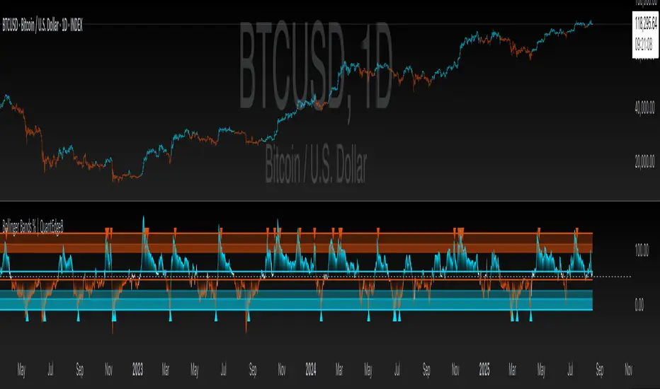
Bollinger Bands % | QuantEdgeB📊 Introducing Bollinger Bands % (BB%) by QuantEdgeB
🛠️ Overview
BB% | QuantEdgeB is a volatility-aware momentum tool that maps price within a Bollinger envelope onto a normalized scale. By letting you choose the base moving average (SMA, EMA, DEMA, TEMA, HMA, ALMA, EHMA, THMA, RMA, WMA, VWMA, T3, LSMA) and even Heikin-Ashi sources, it adapts to your style while keeping readings consistent across symbols and timeframes. Clear thresholds and color-coded visuals make it easy to spot emerging strength, fading moves, and potential mean-reversions.
✨ Key Features
• 🔹 Flexible Baseline
Pick from 12 MA types (plus Heikin-Ashi source option) to tailor responsiveness and smoothness.
• 🔹 Normalized Positioning
Price is expressed as a percentage of the band range, yielding an intuitive 0–100 style read (can exceed in extreme trends).
• 🔹 Actionable Thresholds
Default Long 55 / Short 45 levels provide simple, objective triggers.
• 🔹 Visual Clarity
Color-coded candles, shaded OB/OS zones, and adaptive color themes speed up decision-making.
• 🔹 Ready-to-Alert
Built-in alerts for long/short transitions.
📐 How It Works
1️⃣ Band Construction
A moving average (your choice) defines the midline; volatility (standard deviation) builds upper/lower bands.
2️⃣ Normalization
The indicator measures where price sits between the lower and upper band, scaling that into a bounded oscillator (BB%).
3️⃣ Signal Logic
• ✅ Long when BB% rises above 55 (strength toward the top of the envelope).
• ❌ Short when BB% falls below 45 (weakness toward the bottom).
4️⃣ OB/OS Context
Shaded regions above/below typical ranges highlight exhaustion and potential snap-backs.
⚙️ Custom Settings
• Base MA Type: SMA, EMA, DEMA, TEMA, HMA, ALMA, EHMA, THMA, RMA, WMA, VWMA, T3, LSMA
• Source Mode: Classic price or Heikin-Ashi (close/open/high/hlc3)
• Base Length: default 40
• Band Width: standard deviation-based (2× SD by default)
• Long / Short Thresholds: defaults 55 / 45
• Color Mode: Alpha, MultiEdge, TradingSuite, Premium, Fundamental, Classic, Warm, Cold, Strategy
• Candles & Labels: optional candle coloring and signal markers
👥 Ideal For
✅ Trend Followers — Ride strength as price compresses near the upper band.
✅ Swing/Mean-Reversion Traders — Fade extremes when BB% stretches into OB/OS zones.
✅ Multi-Timeframe Analysts — Compare band position consistently across periods.
✅ System Builders — Use BB% as a normalized feature for strategies and filters.
📌 Conclusion
BB% | QuantEdgeB delivers a clean, normalized read of price versus its volatility envelope—adaptable via rich MA/source options and easy to automate with thresholds and alerts.
🔹 Key Takeaways:
1️⃣ Normalized view of price inside the volatility bands
2️⃣ Flexible baseline (12+ MA choices) and Heikin-Ashi support
3️⃣ Straightforward 55/45 triggers with clear visual context
📌 Disclaimer: Past performance is not indicative of future results. No strategy guarantees success.
📌 Strategic Advice: Always backtest, tune parameters, and align with your risk profile before live trading.
Markov Chain [3D] | FractalystWhat exactly is a Markov Chain?
This indicator uses a Markov Chain model to analyze, quantify, and visualize the transitions between market regimes (Bull, Bear, Neutral) on your chart. It dynamically detects these regimes in real-time, calculates transition probabilities, and displays them as animated 3D spheres and arrows, giving traders intuitive insight into current and future market conditions.
How does a Markov Chain work, and how should I read this spheres-and-arrows diagram?
Think of three weather modes: Sunny, Rainy, Cloudy.
Each sphere is one mode. The loop on a sphere means “stay the same next step” (e.g., Sunny again tomorrow).
The arrows leaving a sphere show where things usually go next if they change (e.g., Sunny moving to Cloudy).
Some paths matter more than others. A more prominent loop means the current mode tends to persist. A more prominent outgoing arrow means a change to that destination is the usual next step.
Direction isn’t symmetric: moving Sunny→Cloudy can behave differently than Cloudy→Sunny.
Now relabel the spheres to markets: Bull, Bear, Neutral.
Spheres: market regimes (uptrend, downtrend, range).
Self‑loop: tendency for the current regime to continue on the next bar.
Arrows: the most common next regime if a switch happens.
How to read: Start at the sphere that matches current bar state. If the loop stands out, expect continuation. If one outgoing path stands out, that switch is the typical next step. Opposite directions can differ (Bear→Neutral doesn’t have to match Neutral→Bear).
What states and transitions are shown?
The three market states visualized are:
Bullish (Bull): Upward or strong-market regime.
Bearish (Bear): Downward or weak-market regime.
Neutral: Sideways or range-bound regime.
Bidirectional animated arrows and probability labels show how likely the market is to move from one regime to another (e.g., Bull → Bear or Neutral → Bull).
How does the regime detection system work?
You can use either built-in price returns (based on adaptive Z-score normalization) or supply three custom indicators (such as volume, oscillators, etc.).
Values are statistically normalized (Z-scored) over a configurable lookback period.
The normalized outputs are classified into Bull, Bear, or Neutral zones.
If using three indicators, their regime signals are averaged and smoothed for robustness.
How are transition probabilities calculated?
On every confirmed bar, the algorithm tracks the sequence of detected market states, then builds a rolling window of transitions.
The code maintains a transition count matrix for all regime pairs (e.g., Bull → Bear).
Transition probabilities are extracted for each possible state change using Laplace smoothing for numerical stability, and frequently updated in real-time.
What is unique about the visualization?
3D animated spheres represent each regime and change visually when active.
Animated, bidirectional arrows reveal transition probabilities and allow you to see both dominant and less likely regime flows.
Particles (moving dots) animate along the arrows, enhancing the perception of regime flow direction and speed.
All elements dynamically update with each new price bar, providing a live market map in an intuitive, engaging format.
Can I use custom indicators for regime classification?
Yes! Enable the "Custom Indicators" switch and select any three chart series as inputs. These will be normalized and combined (each with equal weight), broadening the regime classification beyond just price-based movement.
What does the “Lookback Period” control?
Lookback Period (default: 100) sets how much historical data builds the probability matrix. Shorter periods adapt faster to regime changes but may be noisier. Longer periods are more stable but slower to adapt.
How is this different from a Hidden Markov Model (HMM)?
It sets the window for both regime detection and probability calculations. Lower values make the system more reactive, but potentially noisier. Higher values smooth estimates and make the system more robust.
How is this Markov Chain different from a Hidden Markov Model (HMM)?
Markov Chain (as here): All market regimes (Bull, Bear, Neutral) are directly observable on the chart. The transition matrix is built from actual detected regimes, keeping the model simple and interpretable.
Hidden Markov Model: The actual regimes are unobservable ("hidden") and must be inferred from market output or indicator "emissions" using statistical learning algorithms. HMMs are more complex, can capture more subtle structure, but are harder to visualize and require additional machine learning steps for training.
A standard Markov Chain models transitions between observable states using a simple transition matrix, while a Hidden Markov Model assumes the true states are hidden (latent) and must be inferred from observable “emissions” like price or volume data. In practical terms, a Markov Chain is transparent and easier to implement and interpret; an HMM is more expressive but requires statistical inference to estimate hidden states from data.
Markov Chain: states are observable; you directly count or estimate transition probabilities between visible states. This makes it simpler, faster, and easier to validate and tune.
HMM: states are hidden; you only observe emissions generated by those latent states. Learning involves machine learning/statistical algorithms (commonly Baum–Welch/EM for training and Viterbi for decoding) to infer both the transition dynamics and the most likely hidden state sequence from data.
How does the indicator avoid “repainting” or look-ahead bias?
All regime changes and matrix updates happen only on confirmed (closed) bars, so no future data is leaked, ensuring reliable real-time operation.
Are there practical tuning tips?
Tune the Lookback Period for your asset/timeframe: shorter for fast markets, longer for stability.
Use custom indicators if your asset has unique regime drivers.
Watch for rapid changes in transition probabilities as early warning of a possible regime shift.
Who is this indicator for?
Quants and quantitative researchers exploring probabilistic market modeling, especially those interested in regime-switching dynamics and Markov models.
Programmers and system developers who need a probabilistic regime filter for systematic and algorithmic backtesting:
The Markov Chain indicator is ideally suited for programmatic integration via its bias output (1 = Bull, 0 = Neutral, -1 = Bear).
Although the visualization is engaging, the core output is designed for automated, rules-based workflows—not for discretionary/manual trading decisions.
Developers can connect the indicator’s output directly to their Pine Script logic (using input.source()), allowing rapid and robust backtesting of regime-based strategies.
It acts as a plug-and-play regime filter: simply plug the bias output into your entry/exit logic, and you have a scientifically robust, probabilistically-derived signal for filtering, timing, position sizing, or risk regimes.
The MC's output is intentionally "trinary" (1/0/-1), focusing on clear regime states for unambiguous decision-making in code. If you require nuanced, multi-probability or soft-label state vectors, consider expanding the indicator or stacking it with a probability-weighted logic layer in your scripting.
Because it avoids subjectivity, this approach is optimal for systematic quants, algo developers building backtested, repeatable strategies based on probabilistic regime analysis.
What's the mathematical foundation behind this?
The mathematical foundation behind this Markov Chain indicator—and probabilistic regime detection in finance—draws from two principal models: the (standard) Markov Chain and the Hidden Markov Model (HMM).
How to use this indicator programmatically?
The Markov Chain indicator automatically exports a bias value (+1 for Bullish, -1 for Bearish, 0 for Neutral) as a plot visible in the Data Window. This allows you to integrate its regime signal into your own scripts and strategies for backtesting, automation, or live trading.
Step-by-Step Integration with Pine Script (input.source)
Add the Markov Chain indicator to your chart.
This must be done first, since your custom script will "pull" the bias signal from the indicator's plot.
In your strategy, create an input using input.source()
Example:
//@version=5
strategy("MC Bias Strategy Example")
mcBias = input.source(close, "MC Bias Source")
After saving, go to your script’s settings. For the “MC Bias Source” input, select the plot/output of the Markov Chain indicator (typically its bias plot).
Use the bias in your trading logic
Example (long only on Bull, flat otherwise):
if mcBias == 1
strategy.entry("Long", strategy.long)
else
strategy.close("Long")
For more advanced workflows, combine mcBias with additional filters or trailing stops.
How does this work behind-the-scenes?
TradingView’s input.source() lets you use any plot from another indicator as a real-time, “live” data feed in your own script (source).
The selected bias signal is available to your Pine code as a variable, enabling logical decisions based on regime (trend-following, mean-reversion, etc.).
This enables powerful strategy modularity : decouple regime detection from entry/exit logic, allowing fast experimentation without rewriting core signal code.
Integrating 45+ Indicators with Your Markov Chain — How & Why
The Enhanced Custom Indicators Export script exports a massive suite of over 45 technical indicators—ranging from classic momentum (RSI, MACD, Stochastic, etc.) to trend, volume, volatility, and oscillator tools—all pre-calculated, centered/scaled, and available as plots.
// Enhanced Custom Indicators Export - 45 Technical Indicators
// Comprehensive technical analysis suite for advanced market regime detection
//@version=6
indicator('Enhanced Custom Indicators Export | Fractalyst', shorttitle='Enhanced CI Export', overlay=false, scale=scale.right, max_labels_count=500, max_lines_count=500)
// |----- Input Parameters -----| //
momentum_group = "Momentum Indicators"
trend_group = "Trend Indicators"
volume_group = "Volume Indicators"
volatility_group = "Volatility Indicators"
oscillator_group = "Oscillator Indicators"
display_group = "Display Settings"
// Common lengths
length_14 = input.int(14, "Standard Length (14)", minval=1, maxval=100, group=momentum_group)
length_20 = input.int(20, "Medium Length (20)", minval=1, maxval=200, group=trend_group)
length_50 = input.int(50, "Long Length (50)", minval=1, maxval=200, group=trend_group)
// Display options
show_table = input.bool(true, "Show Values Table", group=display_group)
table_size = input.string("Small", "Table Size", options= , group=display_group)
// |----- MOMENTUM INDICATORS (15 indicators) -----| //
// 1. RSI (Relative Strength Index)
rsi_14 = ta.rsi(close, length_14)
rsi_centered = rsi_14 - 50
// 2. Stochastic Oscillator
stoch_k = ta.stoch(close, high, low, length_14)
stoch_d = ta.sma(stoch_k, 3)
stoch_centered = stoch_k - 50
// 3. Williams %R
williams_r = ta.stoch(close, high, low, length_14) - 100
// 4. MACD (Moving Average Convergence Divergence)
= ta.macd(close, 12, 26, 9)
// 5. Momentum (Rate of Change)
momentum = ta.mom(close, length_14)
momentum_pct = (momentum / close ) * 100
// 6. Rate of Change (ROC)
roc = ta.roc(close, length_14)
// 7. Commodity Channel Index (CCI)
cci = ta.cci(close, length_20)
// 8. Money Flow Index (MFI)
mfi = ta.mfi(close, length_14)
mfi_centered = mfi - 50
// 9. Awesome Oscillator (AO)
ao = ta.sma(hl2, 5) - ta.sma(hl2, 34)
// 10. Accelerator Oscillator (AC)
ac = ao - ta.sma(ao, 5)
// 11. Chande Momentum Oscillator (CMO)
cmo = ta.cmo(close, length_14)
// 12. Detrended Price Oscillator (DPO)
dpo = close - ta.sma(close, length_20)
// 13. Price Oscillator (PPO)
ppo = ta.sma(close, 12) - ta.sma(close, 26)
ppo_pct = (ppo / ta.sma(close, 26)) * 100
// 14. TRIX
trix_ema1 = ta.ema(close, length_14)
trix_ema2 = ta.ema(trix_ema1, length_14)
trix_ema3 = ta.ema(trix_ema2, length_14)
trix = ta.roc(trix_ema3, 1) * 10000
// 15. Klinger Oscillator
klinger = ta.ema(volume * (high + low + close) / 3, 34) - ta.ema(volume * (high + low + close) / 3, 55)
// 16. Fisher Transform
fisher_hl2 = 0.5 * (hl2 - ta.lowest(hl2, 10)) / (ta.highest(hl2, 10) - ta.lowest(hl2, 10)) - 0.25
fisher = 0.5 * math.log((1 + fisher_hl2) / (1 - fisher_hl2))
// 17. Stochastic RSI
stoch_rsi = ta.stoch(rsi_14, rsi_14, rsi_14, length_14)
stoch_rsi_centered = stoch_rsi - 50
// 18. Relative Vigor Index (RVI)
rvi_num = ta.swma(close - open)
rvi_den = ta.swma(high - low)
rvi = rvi_den != 0 ? rvi_num / rvi_den : 0
// 19. Balance of Power (BOP)
bop = (close - open) / (high - low)
// |----- TREND INDICATORS (10 indicators) -----| //
// 20. Simple Moving Average Momentum
sma_20 = ta.sma(close, length_20)
sma_momentum = ((close - sma_20) / sma_20) * 100
// 21. Exponential Moving Average Momentum
ema_20 = ta.ema(close, length_20)
ema_momentum = ((close - ema_20) / ema_20) * 100
// 22. Parabolic SAR
sar = ta.sar(0.02, 0.02, 0.2)
sar_trend = close > sar ? 1 : -1
// 23. Linear Regression Slope
lr_slope = ta.linreg(close, length_20, 0) - ta.linreg(close, length_20, 1)
// 24. Moving Average Convergence (MAC)
mac = ta.sma(close, 10) - ta.sma(close, 30)
// 25. Trend Intensity Index (TII)
tii_sum = 0.0
for i = 1 to length_20
tii_sum += close > close ? 1 : 0
tii = (tii_sum / length_20) * 100
// 26. Ichimoku Cloud Components
ichimoku_tenkan = (ta.highest(high, 9) + ta.lowest(low, 9)) / 2
ichimoku_kijun = (ta.highest(high, 26) + ta.lowest(low, 26)) / 2
ichimoku_signal = ichimoku_tenkan > ichimoku_kijun ? 1 : -1
// 27. MESA Adaptive Moving Average (MAMA)
mama_alpha = 2.0 / (length_20 + 1)
mama = ta.ema(close, length_20)
mama_momentum = ((close - mama) / mama) * 100
// 28. Zero Lag Exponential Moving Average (ZLEMA)
zlema_lag = math.round((length_20 - 1) / 2)
zlema_data = close + (close - close )
zlema = ta.ema(zlema_data, length_20)
zlema_momentum = ((close - zlema) / zlema) * 100
// |----- VOLUME INDICATORS (6 indicators) -----| //
// 29. On-Balance Volume (OBV)
obv = ta.obv
// 30. Volume Rate of Change (VROC)
vroc = ta.roc(volume, length_14)
// 31. Price Volume Trend (PVT)
pvt = ta.pvt
// 32. Negative Volume Index (NVI)
nvi = 0.0
nvi := volume < volume ? nvi + ((close - close ) / close ) * nvi : nvi
// 33. Positive Volume Index (PVI)
pvi = 0.0
pvi := volume > volume ? pvi + ((close - close ) / close ) * pvi : pvi
// 34. Volume Oscillator
vol_osc = ta.sma(volume, 5) - ta.sma(volume, 10)
// 35. Ease of Movement (EOM)
eom_distance = high - low
eom_box_height = volume / 1000000
eom = eom_box_height != 0 ? eom_distance / eom_box_height : 0
eom_sma = ta.sma(eom, length_14)
// 36. Force Index
force_index = volume * (close - close )
force_index_sma = ta.sma(force_index, length_14)
// |----- VOLATILITY INDICATORS (10 indicators) -----| //
// 37. Average True Range (ATR)
atr = ta.atr(length_14)
atr_pct = (atr / close) * 100
// 38. Bollinger Bands Position
bb_basis = ta.sma(close, length_20)
bb_dev = 2.0 * ta.stdev(close, length_20)
bb_upper = bb_basis + bb_dev
bb_lower = bb_basis - bb_dev
bb_position = bb_dev != 0 ? (close - bb_basis) / bb_dev : 0
bb_width = bb_dev != 0 ? (bb_upper - bb_lower) / bb_basis * 100 : 0
// 39. Keltner Channels Position
kc_basis = ta.ema(close, length_20)
kc_range = ta.ema(ta.tr, length_20)
kc_upper = kc_basis + (2.0 * kc_range)
kc_lower = kc_basis - (2.0 * kc_range)
kc_position = kc_range != 0 ? (close - kc_basis) / kc_range : 0
// 40. Donchian Channels Position
dc_upper = ta.highest(high, length_20)
dc_lower = ta.lowest(low, length_20)
dc_basis = (dc_upper + dc_lower) / 2
dc_position = (dc_upper - dc_lower) != 0 ? (close - dc_basis) / (dc_upper - dc_lower) : 0
// 41. Standard Deviation
std_dev = ta.stdev(close, length_20)
std_dev_pct = (std_dev / close) * 100
// 42. Relative Volatility Index (RVI)
rvi_up = ta.stdev(close > close ? close : 0, length_14)
rvi_down = ta.stdev(close < close ? close : 0, length_14)
rvi_total = rvi_up + rvi_down
rvi_volatility = rvi_total != 0 ? (rvi_up / rvi_total) * 100 : 50
// 43. Historical Volatility
hv_returns = math.log(close / close )
hv = ta.stdev(hv_returns, length_20) * math.sqrt(252) * 100
// 44. Garman-Klass Volatility
gk_vol = math.log(high/low) * math.log(high/low) - (2*math.log(2)-1) * math.log(close/open) * math.log(close/open)
gk_volatility = math.sqrt(ta.sma(gk_vol, length_20)) * 100
// 45. Parkinson Volatility
park_vol = math.log(high/low) * math.log(high/low)
parkinson = math.sqrt(ta.sma(park_vol, length_20) / (4 * math.log(2))) * 100
// 46. Rogers-Satchell Volatility
rs_vol = math.log(high/close) * math.log(high/open) + math.log(low/close) * math.log(low/open)
rogers_satchell = math.sqrt(ta.sma(rs_vol, length_20)) * 100
// |----- OSCILLATOR INDICATORS (5 indicators) -----| //
// 47. Elder Ray Index
elder_bull = high - ta.ema(close, 13)
elder_bear = low - ta.ema(close, 13)
elder_power = elder_bull + elder_bear
// 48. Schaff Trend Cycle (STC)
stc_macd = ta.ema(close, 23) - ta.ema(close, 50)
stc_k = ta.stoch(stc_macd, stc_macd, stc_macd, 10)
stc_d = ta.ema(stc_k, 3)
stc = ta.stoch(stc_d, stc_d, stc_d, 10)
// 49. Coppock Curve
coppock_roc1 = ta.roc(close, 14)
coppock_roc2 = ta.roc(close, 11)
coppock = ta.wma(coppock_roc1 + coppock_roc2, 10)
// 50. Know Sure Thing (KST)
kst_roc1 = ta.roc(close, 10)
kst_roc2 = ta.roc(close, 15)
kst_roc3 = ta.roc(close, 20)
kst_roc4 = ta.roc(close, 30)
kst = ta.sma(kst_roc1, 10) + 2*ta.sma(kst_roc2, 10) + 3*ta.sma(kst_roc3, 10) + 4*ta.sma(kst_roc4, 15)
// 51. Percentage Price Oscillator (PPO)
ppo_line = ((ta.ema(close, 12) - ta.ema(close, 26)) / ta.ema(close, 26)) * 100
ppo_signal = ta.ema(ppo_line, 9)
ppo_histogram = ppo_line - ppo_signal
// |----- PLOT MAIN INDICATORS -----| //
// Plot key momentum indicators
plot(rsi_centered, title="01_RSI_Centered", color=color.purple, linewidth=1)
plot(stoch_centered, title="02_Stoch_Centered", color=color.blue, linewidth=1)
plot(williams_r, title="03_Williams_R", color=color.red, linewidth=1)
plot(macd_histogram, title="04_MACD_Histogram", color=color.orange, linewidth=1)
plot(cci, title="05_CCI", color=color.green, linewidth=1)
// Plot trend indicators
plot(sma_momentum, title="06_SMA_Momentum", color=color.navy, linewidth=1)
plot(ema_momentum, title="07_EMA_Momentum", color=color.maroon, linewidth=1)
plot(sar_trend, title="08_SAR_Trend", color=color.teal, linewidth=1)
plot(lr_slope, title="09_LR_Slope", color=color.lime, linewidth=1)
plot(mac, title="10_MAC", color=color.fuchsia, linewidth=1)
// Plot volatility indicators
plot(atr_pct, title="11_ATR_Pct", color=color.yellow, linewidth=1)
plot(bb_position, title="12_BB_Position", color=color.aqua, linewidth=1)
plot(kc_position, title="13_KC_Position", color=color.olive, linewidth=1)
plot(std_dev_pct, title="14_StdDev_Pct", color=color.silver, linewidth=1)
plot(bb_width, title="15_BB_Width", color=color.gray, linewidth=1)
// Plot volume indicators
plot(vroc, title="16_VROC", color=color.blue, linewidth=1)
plot(eom_sma, title="17_EOM", color=color.red, linewidth=1)
plot(vol_osc, title="18_Vol_Osc", color=color.green, linewidth=1)
plot(force_index_sma, title="19_Force_Index", color=color.orange, linewidth=1)
plot(obv, title="20_OBV", color=color.purple, linewidth=1)
// Plot additional oscillators
plot(ao, title="21_Awesome_Osc", color=color.navy, linewidth=1)
plot(cmo, title="22_CMO", color=color.maroon, linewidth=1)
plot(dpo, title="23_DPO", color=color.teal, linewidth=1)
plot(trix, title="24_TRIX", color=color.lime, linewidth=1)
plot(fisher, title="25_Fisher", color=color.fuchsia, linewidth=1)
// Plot more momentum indicators
plot(mfi_centered, title="26_MFI_Centered", color=color.yellow, linewidth=1)
plot(ac, title="27_AC", color=color.aqua, linewidth=1)
plot(ppo_pct, title="28_PPO_Pct", color=color.olive, linewidth=1)
plot(stoch_rsi_centered, title="29_StochRSI_Centered", color=color.silver, linewidth=1)
plot(klinger, title="30_Klinger", color=color.gray, linewidth=1)
// Plot trend continuation
plot(tii, title="31_TII", color=color.blue, linewidth=1)
plot(ichimoku_signal, title="32_Ichimoku_Signal", color=color.red, linewidth=1)
plot(mama_momentum, title="33_MAMA_Momentum", color=color.green, linewidth=1)
plot(zlema_momentum, title="34_ZLEMA_Momentum", color=color.orange, linewidth=1)
plot(bop, title="35_BOP", color=color.purple, linewidth=1)
// Plot volume continuation
plot(nvi, title="36_NVI", color=color.navy, linewidth=1)
plot(pvi, title="37_PVI", color=color.maroon, linewidth=1)
plot(momentum_pct, title="38_Momentum_Pct", color=color.teal, linewidth=1)
plot(roc, title="39_ROC", color=color.lime, linewidth=1)
plot(rvi, title="40_RVI", color=color.fuchsia, linewidth=1)
// Plot volatility continuation
plot(dc_position, title="41_DC_Position", color=color.yellow, linewidth=1)
plot(rvi_volatility, title="42_RVI_Volatility", color=color.aqua, linewidth=1)
plot(hv, title="43_Historical_Vol", color=color.olive, linewidth=1)
plot(gk_volatility, title="44_GK_Volatility", color=color.silver, linewidth=1)
plot(parkinson, title="45_Parkinson_Vol", color=color.gray, linewidth=1)
// Plot final oscillators
plot(rogers_satchell, title="46_RS_Volatility", color=color.blue, linewidth=1)
plot(elder_power, title="47_Elder_Power", color=color.red, linewidth=1)
plot(stc, title="48_STC", color=color.green, linewidth=1)
plot(coppock, title="49_Coppock", color=color.orange, linewidth=1)
plot(kst, title="50_KST", color=color.purple, linewidth=1)
// Plot final indicators
plot(ppo_histogram, title="51_PPO_Histogram", color=color.navy, linewidth=1)
plot(pvt, title="52_PVT", color=color.maroon, linewidth=1)
// |----- Reference Lines -----| //
hline(0, "Zero Line", color=color.gray, linestyle=hline.style_dashed, linewidth=1)
hline(50, "Midline", color=color.gray, linestyle=hline.style_dotted, linewidth=1)
hline(-50, "Lower Midline", color=color.gray, linestyle=hline.style_dotted, linewidth=1)
hline(25, "Upper Threshold", color=color.gray, linestyle=hline.style_dotted, linewidth=1)
hline(-25, "Lower Threshold", color=color.gray, linestyle=hline.style_dotted, linewidth=1)
// |----- Enhanced Information Table -----| //
if show_table and barstate.islast
table_position = position.top_right
table_text_size = table_size == "Tiny" ? size.tiny : table_size == "Small" ? size.small : size.normal
var table info_table = table.new(table_position, 3, 18, bgcolor=color.new(color.white, 85), border_width=1, border_color=color.gray)
// Headers
table.cell(info_table, 0, 0, 'Category', text_color=color.black, text_size=table_text_size, bgcolor=color.new(color.blue, 70))
table.cell(info_table, 1, 0, 'Indicator', text_color=color.black, text_size=table_text_size, bgcolor=color.new(color.blue, 70))
table.cell(info_table, 2, 0, 'Value', text_color=color.black, text_size=table_text_size, bgcolor=color.new(color.blue, 70))
// Key Momentum Indicators
table.cell(info_table, 0, 1, 'MOMENTUM', text_color=color.purple, text_size=table_text_size, bgcolor=color.new(color.purple, 90))
table.cell(info_table, 1, 1, 'RSI Centered', text_color=color.purple, text_size=table_text_size)
table.cell(info_table, 2, 1, str.tostring(rsi_centered, '0.00'), text_color=color.purple, text_size=table_text_size)
table.cell(info_table, 0, 2, '', text_color=color.blue, text_size=table_text_size)
table.cell(info_table, 1, 2, 'Stoch Centered', text_color=color.blue, text_size=table_text_size)
table.cell(info_table, 2, 2, str.tostring(stoch_centered, '0.00'), text_color=color.blue, text_size=table_text_size)
table.cell(info_table, 0, 3, '', text_color=color.red, text_size=table_text_size)
table.cell(info_table, 1, 3, 'Williams %R', text_color=color.red, text_size=table_text_size)
table.cell(info_table, 2, 3, str.tostring(williams_r, '0.00'), text_color=color.red, text_size=table_text_size)
table.cell(info_table, 0, 4, '', text_color=color.orange, text_size=table_text_size)
table.cell(info_table, 1, 4, 'MACD Histogram', text_color=color.orange, text_size=table_text_size)
table.cell(info_table, 2, 4, str.tostring(macd_histogram, '0.000'), text_color=color.orange, text_size=table_text_size)
table.cell(info_table, 0, 5, '', text_color=color.green, text_size=table_text_size)
table.cell(info_table, 1, 5, 'CCI', text_color=color.green, text_size=table_text_size)
table.cell(info_table, 2, 5, str.tostring(cci, '0.00'), text_color=color.green, text_size=table_text_size)
// Key Trend Indicators
table.cell(info_table, 0, 6, 'TREND', text_color=color.navy, text_size=table_text_size, bgcolor=color.new(color.navy, 90))
table.cell(info_table, 1, 6, 'SMA Momentum %', text_color=color.navy, text_size=table_text_size)
table.cell(info_table, 2, 6, str.tostring(sma_momentum, '0.00'), text_color=color.navy, text_size=table_text_size)
table.cell(info_table, 0, 7, '', text_color=color.maroon, text_size=table_text_size)
table.cell(info_table, 1, 7, 'EMA Momentum %', text_color=color.maroon, text_size=table_text_size)
table.cell(info_table, 2, 7, str.tostring(ema_momentum, '0.00'), text_color=color.maroon, text_size=table_text_size)
table.cell(info_table, 0, 8, '', text_color=color.teal, text_size=table_text_size)
table.cell(info_table, 1, 8, 'SAR Trend', text_color=color.teal, text_size=table_text_size)
table.cell(info_table, 2, 8, str.tostring(sar_trend, '0'), text_color=color.teal, text_size=table_text_size)
table.cell(info_table, 0, 9, '', text_color=color.lime, text_size=table_text_size)
table.cell(info_table, 1, 9, 'Linear Regression', text_color=color.lime, text_size=table_text_size)
table.cell(info_table, 2, 9, str.tostring(lr_slope, '0.000'), text_color=color.lime, text_size=table_text_size)
// Key Volatility Indicators
table.cell(info_table, 0, 10, 'VOLATILITY', text_color=color.yellow, text_size=table_text_size, bgcolor=color.new(color.yellow, 90))
table.cell(info_table, 1, 10, 'ATR %', text_color=color.yellow, text_size=table_text_size)
table.cell(info_table, 2, 10, str.tostring(atr_pct, '0.00'), text_color=color.yellow, text_size=table_text_size)
table.cell(info_table, 0, 11, '', text_color=color.aqua, text_size=table_text_size)
table.cell(info_table, 1, 11, 'BB Position', text_color=color.aqua, text_size=table_text_size)
table.cell(info_table, 2, 11, str.tostring(bb_position, '0.00'), text_color=color.aqua, text_size=table_text_size)
table.cell(info_table, 0, 12, '', text_color=color.olive, text_size=table_text_size)
table.cell(info_table, 1, 12, 'KC Position', text_color=color.olive, text_size=table_text_size)
table.cell(info_table, 2, 12, str.tostring(kc_position, '0.00'), text_color=color.olive, text_size=table_text_size)
// Key Volume Indicators
table.cell(info_table, 0, 13, 'VOLUME', text_color=color.blue, text_size=table_text_size, bgcolor=color.new(color.blue, 90))
table.cell(info_table, 1, 13, 'Volume ROC', text_color=color.blue, text_size=table_text_size)
table.cell(info_table, 2, 13, str.tostring(vroc, '0.00'), text_color=color.blue, text_size=table_text_size)
table.cell(info_table, 0, 14, '', text_color=color.red, text_size=table_text_size)
table.cell(info_table, 1, 14, 'EOM', text_color=color.red, text_size=table_text_size)
table.cell(info_table, 2, 14, str.tostring(eom_sma, '0.000'), text_color=color.red, text_size=table_text_size)
// Key Oscillators
table.cell(info_table, 0, 15, 'OSCILLATORS', text_color=color.purple, text_size=table_text_size, bgcolor=color.new(color.purple, 90))
table.cell(info_table, 1, 15, 'Awesome Osc', text_color=color.blue, text_size=table_text_size)
table.cell(info_table, 2, 15, str.tostring(ao, '0.000'), text_color=color.blue, text_size=table_text_size)
table.cell(info_table, 0, 16, '', text_color=color.red, text_size=table_text_size)
table.cell(info_table, 1, 16, 'Fisher Transform', text_color=color.red, text_size=table_text_size)
table.cell(info_table, 2, 16, str.tostring(fisher, '0.000'), text_color=color.red, text_size=table_text_size)
// Summary Statistics
table.cell(info_table, 0, 17, 'SUMMARY', text_color=color.black, text_size=table_text_size, bgcolor=color.new(color.gray, 70))
table.cell(info_table, 1, 17, 'Total Indicators: 52', text_color=color.black, text_size=table_text_size)
regime_color = rsi_centered > 10 ? color.green : rsi_centered < -10 ? color.red : color.gray
regime_text = rsi_centered > 10 ? "BULLISH" : rsi_centered < -10 ? "BEARISH" : "NEUTRAL"
table.cell(info_table, 2, 17, regime_text, text_color=regime_color, text_size=table_text_size)
This makes it the perfect “indicator backbone” for quantitative and systematic traders who want to prototype, combine, and test new regime detection models—especially in combination with the Markov Chain indicator.
How to use this script with the Markov Chain for research and backtesting:
Add the Enhanced Indicator Export to your chart.
Every calculated indicator is available as an individual data stream.
Connect the indicator(s) you want as custom input(s) to the Markov Chain’s “Custom Indicators” option.
In the Markov Chain indicator’s settings, turn ON the custom indicator mode.
For each of the three custom indicator inputs, select the exported plot from the Enhanced Export script—the menu lists all 45+ signals by name.
This creates a powerful, modular regime-detection engine where you can mix-and-match momentum, trend, volume, or custom combinations for advanced filtering.
Backtest regime logic directly.
Once you’ve connected your chosen indicators, the Markov Chain script performs regime detection (Bull/Neutral/Bear) based on your selected features—not just price returns.
The regime detection is robust, automatically normalized (using Z-score), and outputs bias (1, -1, 0) for plug-and-play integration.
Export the regime bias for programmatic use.
As described above, use input.source() in your Pine Script strategy or system and link the bias output.
You can now filter signals, control trade direction/size, or design pairs-trading that respect true, indicator-driven market regimes.
With this framework, you’re not limited to static or simplistic regime filters. You can rigorously define, test, and refine what “market regime” means for your strategies—using the technical features that matter most to you.
Optimize your signal generation by backtesting across a universe of meaningful indicator blends.
Enhance risk management with objective, real-time regime boundaries.
Accelerate your research: iterate quickly, swap indicator components, and see results with minimal code changes.
Automate multi-asset or pairs-trading by integrating regime context directly into strategy logic.
Add both scripts to your chart, connect your preferred features, and start investigating your best regime-based trades—entirely within the TradingView ecosystem.
References & Further Reading
Ang, A., & Bekaert, G. (2002). “Regime Switches in Interest Rates.” Journal of Business & Economic Statistics, 20(2), 163–182.
Hamilton, J. D. (1989). “A New Approach to the Economic Analysis of Nonstationary Time Series and the Business Cycle.” Econometrica, 57(2), 357–384.
Markov, A. A. (1906). "Extension of the Limit Theorems of Probability Theory to a Sum of Variables Connected in a Chain." The Notes of the Imperial Academy of Sciences of St. Petersburg.
Guidolin, M., & Timmermann, A. (2007). “Asset Allocation under Multivariate Regime Switching.” Journal of Economic Dynamics and Control, 31(11), 3503–3544.
Murphy, J. J. (1999). Technical Analysis of the Financial Markets. New York Institute of Finance.
Brock, W., Lakonishok, J., & LeBaron, B. (1992). “Simple Technical Trading Rules and the Stochastic Properties of Stock Returns.” Journal of Finance, 47(5), 1731–1764.
Zucchini, W., MacDonald, I. L., & Langrock, R. (2017). Hidden Markov Models for Time Series: An Introduction Using R (2nd ed.). Chapman and Hall/CRC.
On Quantitative Finance and Markov Models:
Lo, A. W., & Hasanhodzic, J. (2009). The Heretics of Finance: Conversations with Leading Practitioners of Technical Analysis. Bloomberg Press.
Patterson, S. (2016). The Man Who Solved the Market: How Jim Simons Launched the Quant Revolution. Penguin Press.
TradingView Pine Script Documentation: www.tradingview.com
TradingView Blog: “Use an Input From Another Indicator With Your Strategy” www.tradingview.com
GeeksforGeeks: “What is the Difference Between Markov Chains and Hidden Markov Models?” www.geeksforgeeks.org
What makes this indicator original and unique?
- On‑chart, real‑time Markov. The chain is drawn directly on your chart. You see the current regime, its tendency to stay (self‑loop), and the usual next step (arrows) as bars confirm.
- Source‑agnostic by design. The engine runs on any series you select via input.source() — price, your own oscillator, a composite score, anything you compute in the script.
- Automatic normalization + regime mapping. Different inputs live on different scales. The script standardizes your chosen source and maps it into clear regimes (e.g., Bull / Bear / Neutral) without you micromanaging thresholds each time.
- Rolling, bar‑by‑bar learning. Transition tendencies are computed from a rolling window of confirmed bars. What you see is exactly what the market did in that window.
- Fast experimentation. Switch the source, adjust the window, and the Markov view updates instantly. It’s a rapid way to test ideas and feel regime persistence/switch behavior.
Integrate your own signals (using input.source())
- In settings, choose the Source . This is powered by input.source() .
- Feed it price, an indicator you compute inside the script, or a custom composite series.
- The script will automatically normalize that series and process it through the Markov engine, mapping it to regimes and updating the on‑chart spheres/arrows in real time.
Credits:
Deep gratitude to @RicardoSantos for both the foundational Markov chain processing engine and inspiring open-source contributions, which made advanced probabilistic market modeling accessible to the TradingView community.
Special thanks to @Alien_Algorithms for the innovative and visually stunning 3D sphere logic that powers the indicator’s animated, regime-based visualization.
Disclaimer
This tool summarizes recent behavior. It is not financial advice and not a guarantee of future results.
