Statistics: High & Low timings of custom session; 1yr historyGet statistics of the Session High and Session Low timings for any custom session; based on around 1yr of data.
//Purpose:
-To get data on the 'time of day' tendencies of an asset.
-Narrow in on a custom defined session and get statistics on that session.
//Notes:
-Input times are always in New York time (but changing the timezone after setting WILL adust both table stats and background highlight correctly.
-For particularly long sessions, make sure text size is set to 'tiny' (very long vertical table), or adjust table to display horizontally.
-You'll notice most assets show higher readings around NY equities open (9:30am NY time). Other assets will have 'hot-spots' at other times too.
-Timings represent the beginning of a 15m candle. i.e. reading for 15:45 represents a high occurring between 15:45 and 1600.
-Premium users should get 20k bars => around 1year's worth of data on a 15minute chart. Days of history is displayed in the top left corner of the table.
//Limitations
-only designed and working on 15minute timeframe (to gather a full year of meaningful/comparable % stats, need 15minute 'buckets' of time.
-sessions cannot cross through midnight, or start at midnight (00:15 is ok). 00:15 >> 23:45 is the max session length. On BTC, same applies but 01:00 instead of midnight (all in NY time).
-if your session crosses through 'dead time' (e.g. 17:00-18:00 S&P NY time); table will correctly omit these non-existent candles, but it will add on the missing hour before the start time.
//Cautionary note:
-Since markets are not uncommonly in a trending state when your defined session starts or ends, the high/low timings % readings for start and end of session may be misleadingly high. Try to look for unusually high readings that are not at the start/end of your session.
Wheat (ZW1!) 15min chart; Table displayed vertically:
Nasdaq (NQ1!) 15m chart; Table displayed horizontally and with smaller text to view a very long custom session:
Cari dalam skrip untuk "沪深主板45度上升的股票"

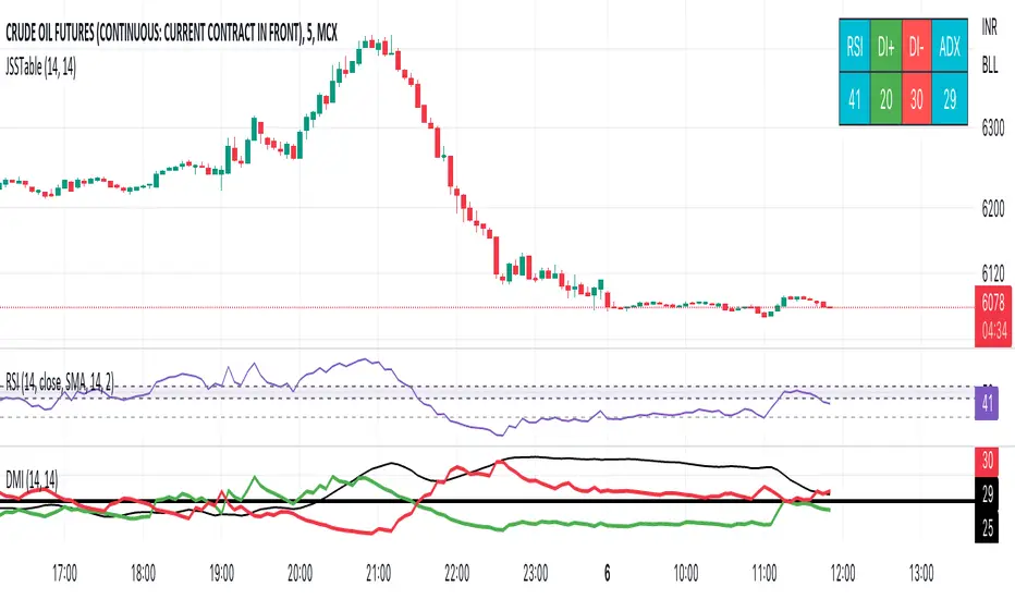
JSS Table - RSI, DI+, DI-, ADXSimple table to show the values for indicators which can be used to initiate trades:
RSI: Long above 55 // Short below 45 // Choppy between 45-55
DI+: Long above 25
DI-: Short above 25
Note when to avoid trend trades:
- If DI+ and DI- are both below 25 then market is choppy
- If RSI is between 45-55 then market is choppy
Ichimoku Cloud with ADX (By Coinrule)The Ichimoku Cloud is a collection of technical indicators that show support and resistance levels, as well as momentum and trend direction. It does this by taking multiple averages and plotting them on a chart. It also uses these figures to compute a “cloud” that attempts to forecast where the price may find support or resistance in the future.
The Ichimoku Cloud was developed by Goichi Hosoda, a Japanese journalist, and published in the late 1960s. It provides more data points than the standard candlestick chart. While it seems complicated at first glance, those familiar with how to read the charts often find it easy to understand with well-defined trading signals.
The Ichimoku Cloud is composed of five lines or calculations, two of which comprise a cloud where the difference between the two lines is shaded in.
The lines include a nine-period average, a 26-period average, an average of those two averages, a 52-period average, and a lagging closing price line.
The cloud is a key part of the indicator. When the price is below the cloud, the trend is down. When the price is above the cloud, the trend is up.
The above trend signals are strengthened if the cloud is moving in the same direction as the price. For example, during an uptrend, the top of the cloud is moving up, or during a downtrend, the bottom of the cloud is moving down.
DMI is simple to interpret. When +DI > - DI, it means the price is trending up. On the other hand, when -DI > +DI , the trend is weak or moving on the downside. The ADX does not give an indication about the direction but about the strength of the trend.
Typically values of ADX above 25 mean that the trend is steeply moving up or down, based on the -DI and +D positioning. This script aims to capture swings in the DMI, and thus, in the trend of the asset, using a contrarian approach.
Trading on high values of ADX , the strategy tries to spot extremely oversold and overbought conditions. Values of ADX above 45 may suggest that the trend has overextended and is may be about to reverse.
This strategy combines the Ichimoku Cloud with the ADX indicator to better enter trades.
Long/Short orders are placed when these basic signals are triggered.
Long Position:
Tenkan-Sen is above the Kijun-Sen
Chikou-Span is above the close of 26 bars ago
Close is above the Kumo Cloud
MACD line crosses over the signal line
-DI is greater than +DI
ADX is greater than 45
Short Position:
Tenkan-Sen is below the Kijun-Sen
Chikou-Span is below the close of 26 bars ago
Close is below the Kumo Cloud
MACD line crosses under the signal line
+DI is greater than -DI
ADX is less than 45
The script is backtested from 1 January 2022 and provides good returns.
The strategy assumes each order is using 30% of the available coins to make the results more realistic and to simulate you only ran this strategy on 30% of your holdings. A trading fee of 0.1% is also taken into account and is aligned to the base fee applied on Binance.
This script also works well on MATIC (15m timeframe), ETH (5m timeframe), and SOL (15m timeframe).
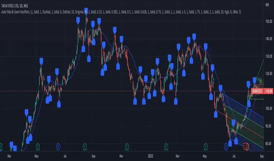
PrasiGanFanFibntroduction
This is a combination of Fibonacci and Gann fan /retracements.
The script can automatically draw as many:
Fibonacci Retracements
Fibonacci Fan
Gann Retracements
Gann Fan
as the user requires on the chart. Each level set or fan consists of 7 lines based on the most important ratios of Fibonacci/ Gann .
Basics
What are Fibonacci retracements?
Fibonacci retracement levels are horizontal lines that indicate where support and resistance are likely to occur. They stem from Fibonacci’s sequence. Each level is associated with a percentage which is how much of a prior move the price has retraced. The Fibonacci retracement levels are 23.6%, 38.2%, 61.8%, and 78.6%. While not officially a Fibonacci ratio, 50% is also used. The indicator is useful because it can be drawn between any two significant price points, such as a high and a low. The indicator will then create the levels between those two points.
What are Gann retracements?
A developer of technical analysis and trading was W.D. Gann . Gann theory expects a normal retracement of 50 percent. This means that under normal selling pressure, the stock price will decline half the amount of its most recent rise, and vice versa. It also suggests that retracements occur at the halfway point of a move, such as 25 percent (half of 50 percent), 12.5 percent (half of 25 percent), and so on.
What is Fibonacci fan?
Fibonacci fan is a set of sequential trend lines drawn from a trough or peak through a set of points dictated by Fibonacci retracements. The first step to create it is to draw a trend line covering the local lowest and highest prices of a security. To reach retracement levels, the trader divides the difference in price at the low and high end by ratios determined by the Fibonacci series. The lines formed by connecting the starting point for the base trend line and each retracement level create the Fibonacci fan.
What is Gann fan?
A Gann fan consists of a series of lines called Gann angles. These angles are superimposed over a price chart to show potential support and resistance levels. The resulting image is supposed to help technical analysts predict price changes. Gann believed the 45-degree angle to be most important, but the Gann fan also draws angles at degrees like 75, 63.75, 26.25 and 15. The Gann fan originates at a low or high point. The resulting lines show areas of potential future support and resistance . The 45-degree line is known as the 1:1 line because the price will rise or fall at a 45-degree angle when the price moves up/down one unit for each unit of time. All other lines in the Gann fan are drawn above and below the 1:1 line. The other angles are associated with 2:1, 3:1, 4:1, 8:1 and 1:8, 1:4, 1:3, and 1:2 time-to-price moves.
Challenges
The most of the time I dedicated to writing this script has been spent on handling these problems:
1. Finding Local Highest/Lowest Prices
In order to draw Fibonacci and Gann fan /retracements, it's necessary to find local highest and lowest price points (Extrema) on the chart. As this could be so challenging, most traders and coders draw the lines covering the low and high prices over a given period of time or a limited number of bars back instead. I already wrote an indicator using this approach (Auto Fibonacci Combo).
In this new script I tried to find the exact highest and lowest prices based on this idea that: if a high point is formed lower than previous high which was after a lowest point, then that previous one was the local highest point, and vice versa if a low point is formed higher than previous low which was after a highest point, then that previous one was the local lowest point. So logically an extremum price on the chart won't be found until the next high/low point is formed.
2. Finding Proper Chart Scale for Gann Fan
Based on the theory, Gann angles are sensitive to the chart price scale and in order to have the right angles, the chart must be made with the proper scale. J.A. Hyerczyk in his book "Pattern, Price & Time - Using Gann Theory in Technical Analysis" suggests that the easiest way to determine the scale of a market is by taking the difference between top-to-top and bottom-to-bottom and dividing it by the time it took the market to move from top to top and bottom to bottom.
Thus on a properly constructed chart, the basic equation for calculating Gann angles is: Price * Time.
3. Drawing Fans and Relocating Fan Labels at Each New Bar in Pine (A Programming-Related Subject)
To do this, I used linear equations and line slopes. Of course it was so complicated and exhausting, but finally I overcame that thanks to my genius cousin.
Settings and Usage
By default, the script shows detected extremum points plus 1 Fibonacci fan, 1 Gann fan , 1 set of Fibonacci retracements and no Gann retracements on the chart. All of these could be changed in the indicator settings beside the color and transparency of each line.
Feel free to use this and send me your thoughts!
Ultimate IndicatorThis is a combination of all the price chart indicators I frequently switch between. It contains my day time highlighter (for day trading), multi-timeframe long-term trend indicator for current commodity in the bottom right, customizable trend EMA which also has multi-timeframe drawing capabilities, VWAP, customizable indicators with separate settings from the trend indicator including: EMA, HL2 over time, Donchian Channels, Keltner Channels, Bollinger Bands, and Super Trend. The settings for these are right below the trend settings and can have their length and multiplier adjusted. All of those also have multi-timeframe capabilities separate from the trend multi-time settings.
The Day Trade Highlight option will draw faint yellow between 9:15-9:25, red between 9:25-9:45, yellow between 9:45-10:05. There will be one white background at 9:30am to show the opening of the market. while the market is open there will be a very faint blue background. For the end of the day there will be yellow between 15:45-15:50, red between 15:50-16:00, and yellow between 16:00-16:05. During the night hours, there is no coloring. The purpose of this highlight is to show the opening / closing times of the market and the hot times for large moves.
The indicators can also be colored in the following ways:
1. Simple = Makes all colors for the indicator Gray
2. Trend = Will use the Donchian Channels to get the short-trend direction and by default will color the short-term direction as Blue or Red. Unless using Super Trend, the Donchian Channel is used to find short-term trend direction.
3. Trend Adv = Will use the Donchian Channels to get the short-trend direction and by default will color the short-term direction as Blue or Red. Unless using Super Trend, the Donchian Channel is used to find short-term trend direction. If there is a short-term up-trend during a long-term down-trend, the Blue will become Navy. If short-term down-trend during long-term up-trend, the Red will be Brown.
4. Squeeze = Compares the Bollinger Bands width to the Keltner Channels width and will color based on relative squeeze of the market: Teal = no squeeze. Yellow = little squeeze. Red = decent squeeze. White = huge squeeze. if you do not understand this one, try drawing the Bollinger Bands while using the Squeeze color option and it should become more apparent how this works. I also recommend leaving the length and multiplier to the default 20 and 2 if using this setting and only changing the timeframe to get longer/shorter lengths as I've seen that changing the length or multiplier can more or less make it not work at all.
Along with the indicator settings are options to draw lines/labels/fills for the indicator. I enjoy having only fills for a cleaner look.
The Labels option will show Buy/Sell signals when the short-term trend flips to agree with the long-term trend.
The Trend Bars option will do the same as the Labels option but instead will color the bars white when a Buy/Sell option is given.
The Range Bars option shows will color a bar white when the Close of a candle is outside of a respective ranging indicator option (Bollinger or Keltner).
The Trend Bars will draw white candles no matter which indicator selection you make (even "Off"). However, Range Bars will only draw white when either Bollinger or Keltner are selected.
The Donchian Channels and Super Trend are trending indicators and should be used during trending markets. I like to use the MACD in conjunction with these indicators for possibly earlier entries.
The Bollinger Bands and Keltner Channel are ranging indicators and should be used during ranging markets. I like to use the RSI in conjunction with these indicators and will use 60/40 for overbought and oversold areas rather than 70/30. During a range, I wait for an overbought or oversold indication and will buy/sell when it crosses back into the middle area and close my position when it touches the opposite band.
I have a MACD/RSI combination indicator if you'd like that as well :D
As always, trade at your own risk. This is not some secret indicator that will 100% win. As always, the trades you see in the picture use a 1:1.5 or 1:2 risk to reward ratio, for today (August 8, 2022) it won 5/6 times with one trade still open at the end of the day. Manage your account correctly and you'll win in the long term. Hit me up with any questions or suggestions. Happy Trading!

Auto Fibonacci and Gann Fan/Retracements ComboIntroduction
This is a combination of Fibonacci and Gann fan/retracements.
The script can automatically draw as many:
Fibonacci Retracements
Fibonacci Fan
Gann Retracements
Gann Fan
as the user requires on the chart. Each level set or fan consists of 7 lines based on the most important ratios of Fibonacci/Gann.
Basics
What are Fibonacci retracements?
Fibonacci retracement levels are horizontal lines that indicate where support and resistance are likely to occur. They stem from Fibonacci’s sequence. Each level is associated with a percentage which is how much of a prior move the price has retraced. The Fibonacci retracement levels are 23.6%, 38.2%, 61.8%, and 78.6%. While not officially a Fibonacci ratio, 50% is also used. The indicator is useful because it can be drawn between any two significant price points, such as a high and a low. The indicator will then create the levels between those two points.
What are Gann retracements?
A developer of technical analysis and trading was W.D. Gann. Gann theory expects a normal retracement of 50 percent. This means that under normal selling pressure, the stock price will decline half the amount of its most recent rise, and vice versa. It also suggests that retracements occur at the halfway point of a move, such as 25 percent (half of 50 percent), 12.5 percent (half of 25 percent), and so on.
What is Fibonacci fan?
Fibonacci fan is a set of sequential trend lines drawn from a trough or peak through a set of points dictated by Fibonacci retracements. The first step to create it is to draw a trend line covering the local lowest and highest prices of a security. To reach retracement levels, the trader divides the difference in price at the low and high end by ratios determined by the Fibonacci series. The lines formed by connecting the starting point for the base trend line and each retracement level create the Fibonacci fan.
What is Gann fan?
A Gann fan consists of a series of lines called Gann angles. These angles are superimposed over a price chart to show potential support and resistance levels. The resulting image is supposed to help technical analysts predict price changes. Gann believed the 45-degree angle to be most important, but the Gann fan also draws angles at degrees like 75, 63.75, 26.25 and 15. The Gann fan originates at a low or high point. The resulting lines show areas of potential future support and resistance. The 45-degree line is known as the 1:1 line because the price will rise or fall at a 45-degree angle when the price moves up/down one unit for each unit of time. All other lines in the Gann fan are drawn above and below the 1:1 line. The other angles are associated with 2:1, 3:1, 4:1, 8:1 and 1:8, 1:4, 1:3, and 1:2 time-to-price moves.
Challenges
The most of the time I dedicated to writing this script has been spent on handling these problems:
1. Finding Local Highest/Lowest Prices
In order to draw Fibonacci and Gann fan/retracements, it's necessary to find local highest and lowest price points (Extrema) on the chart. As this could be so challenging, most traders and coders draw the lines covering the low and high prices over a given period of time or a limited number of bars back instead. I already wrote an indicator using this approach ( Auto Fibonacci Combo ).
In this new script I tried to find the exact highest and lowest prices based on this idea that: if a high point is formed lower than previous high which was after a lowest point, then that previous one was the local highest point, and vice versa if a low point is formed higher than previous low which was after a highest point, then that previous one was the local lowest point. So logically an extremum price on the chart won't be found until the next high/low point is formed.
2. Finding Proper Chart Scale for Gann Fan
Based on the theory, Gann angles are sensitive to the chart price scale and in order to have the right angles, the chart must be made with the proper scale. J.A. Hyerczyk in his book "Pattern, Price & Time - Using Gann Theory in Technical Analysis" suggests that the easiest way to determine the scale of a market is by taking the difference between top-to-top and bottom-to-bottom and dividing it by the time it took the market to move from top to top and bottom to bottom.
Thus on a properly constructed chart, the basic equation for calculating Gann angles is: Price * Time.
3. Drawing Fans and Relocating Fan Labels at Each New Bar in Pine (A Programming-Related Subject)
To do this, I used linear equations and line slopes. Of course it was so complicated and exhausting, but finally I overcame that thanks to my genius cousin.
Settings and Usage
By default, the script shows detected extremum points plus 1 Fibonacci fan, 1 Gann fan, 1 set of Fibonacci retracements and no Gann retracements on the chart. All of these could be changed in the indicator settings beside the color and transparency of each line.
Feel free to use this and send me your thoughts!

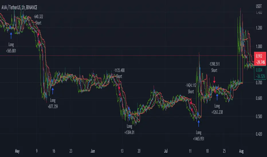
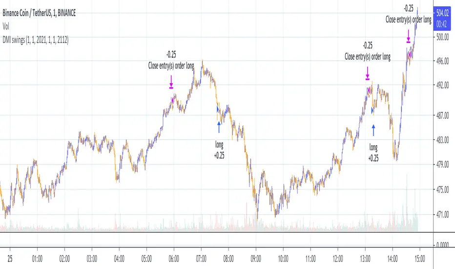
DMI Swings (by Coinrule)The Directional Movement Index is a handy indicator that helps catch the direction in which the price of an asset is moving. It compares the prior highs and lows to draw three lines:
Positive directional line (+DI)
Negative directional line (-DI)
Average direction index (ADX)
DMI is simple to interpret. When +DI > - DI, it means the price is trending up. On the other hand, when -DI > +DI, the trend is weak or moving on the downside.
The ADX does not give an indication about the direction but about the strength of the trend.
Typically values of ADX above 25 mean that the trend is steeply moving up or down, based on the -DI and +D positioning. This script aims to capture swings in the DMI, and thus, in the trend of the asset, using a contrarian approach.
ENTRY
-DI is greater than +DI
ADX is greater than 45
EXIT
+DI is greater than -DI
ADX is greater than 45
Trading on high values of ADX, the strategy tries to spot extremely oversold and overbought conditions. Values of ADX above 45 may suggest that the trend has overextended and is may be about to reverse.
Our backtests suggest that this script performs well for very short-term scalping strategies on low time frames, such as the 1-minute.
The script considers a 0.1% trading fee to make results more realistic to those you can expect from live market conditions. So realistically, live results should be similar to backtested results.
You can plug this script directly into your crypto exchange using TradingView Signals on Coinrule.
Trade Safely!
Sexy RSI for sexy tradersHello fellow sexy traders.
I was tired of constantly having to add my own horizontals/MAs to the default RSI so I decided to make this modification.
The default settings include channels from 40-80 (green horizontals) for a bullish range, and 20-60 (red horizontals) for the bearish range.
Also includes white line at 50 level, and blue horizontals at extremes (90 and 10).
If RSI stays in one of the red or green range that can signify the trend direction, as directed by Andrew Cardwell (inventor of the RSI).
If you wish for other levels to be included, just let me know! Comment on here or dm me on twitter @boss_charts and I can add the settings for you, so all you have to do is click a button and it will set it to your desired config. I want this to be a tool that is useful for heavy traders to save them time.
Additionally, in order to tell the level of the RSI and how overextended it might be, I added the setting for the RSI to change color depending on its level. Current settings are as follows:
Normal RSI (30-70) = PURPLE
Conventional Overbought/Oversold (30-20 + 70-80) = RED
1st extended (20-15 + 80-85) = PINK
2nd extended (15-10 + 85-90) = ORANGE
VERY EXTENDED (<10 + >90) = YELLOW
That way you can get an idea of how drastic a move is by the color alone. According to Dr. Cardwell, a drastic move to over/under extended can be a sign of strength.
Finally, there are the default MAs added that Mr. Cardwell defines as useful for defining the trend. These being the 9 MA and 45 EMA/WMA.
The strategy with these is to have the MAs on both price and RSI. If the 9MA is above the 45 MA on both price and RSI, then this is bullish and you can look for longs.
Conversely, if the 9 is below the 45 on both RSI and price that is bearish, and you can look for shorts.
I added the background color change for the points where the MAs cross each other, so you do not have to have the MAs fogging up your charts to know where they are relative to one another. This is similar to my MA cross indicator which contains the same functionality.
Never financial advice. Backtest it for yourself and find MA configurations that work for you.
Enjoy! Feel free to send feedback/requests whenever.

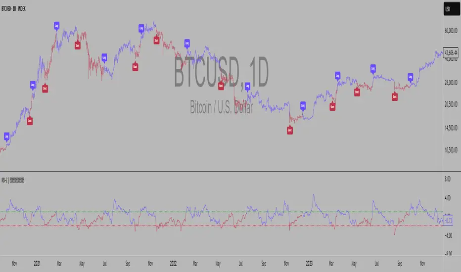
CM Stochastic POP Method 2-Jake Bernstein_V1Yesterday Jake Bernstein authorized me to post his updated results with the Stochastic Pop Trading System he developed many years ago.
You can take a look at the Original System with Updated Settings at
This indicator is a different set of rules Jake mentioned in the PDF he allowed me to post.
To view the PDF use this link:
dl.dropboxusercontent.com
Today we’re releasing the version described in the PDF that uses the StochK values of 55, 50, and 45. The rules are discussed in the PDF but here is a simple breakdown:
Enter Long when StochK is below 50 and Crosses Above 55
Exit Long on Cross Below 55
Enter Short when StochK is Above 50 and crosses Below 45
Exit Short on Cross Above 45
Two Important Items to understand about this method:
To code the rules Precisely we need a function that will be available when Strategy Capabilities are released on TradingView.
There is one of Jakes Profit Maximizing Strategies that needs to be integrated with this code…which again we need the Strategy based Function that will be coming soon.
To Compare this system to the Stochastic Pop Method 1 System shown yesterday at I used the same Symbol and dates for you to compare…but remember to give this Method 2 System a Fair Look/Evaluation…we need the Soon To Be Released…TradingView Strategy Capabilities.
BackTesting Results Example: EUR-USD Daily Chart Since 01/01/2005
Strategy 1 – Stochastic Pop Method 2 System:
Go Long When Stochasticis below 50 and Crosses Above 55. Go Short When Stochastic is above 50 and Crosses Below 45. Exit Long/Short When Stochastic has a Reverse Cross of Entry Value.
Results:
Total Trades = 151
Profit = 40,758 Pips
Win% = 37.1%
Profit Factor = 1.26
Avg Trade = 270 Pips Profit
***Most Consecutive Wins = 4 ... Most Consecutive Losses = 7
Strategy 2:
Rules - Proprietary Optimization Jake Will Teach. Only Added 1 Additional Exit Rule.
Results:
Total Trades = 151
Profit = 60.305 Pips
Win% = 37.1%
Profit Factor = 1.38
Avg Trade = 399 Pips Profit
***Most Consecutive Wins = 4 ... Most Consecutive Losses = 7
Indicator Includes:
-Ability to Color Candles (CheckBox In Inputs Tab)
Green = Long Trade
Blue = No Trade
Red = Short Trade
Jake Bernstein will be a contributor on TradingView when Backtesting/Strategies are released. Jake is one of the Top Trading System Developers in the world with 45+ years experience and he is going to teach TradingView.com’s community how to create Trading Systems and how to Optimize the correct way.
Link To PDF:
dl.dropboxusercontent.com
Link to Original Version of Indicator with Updated Settings.

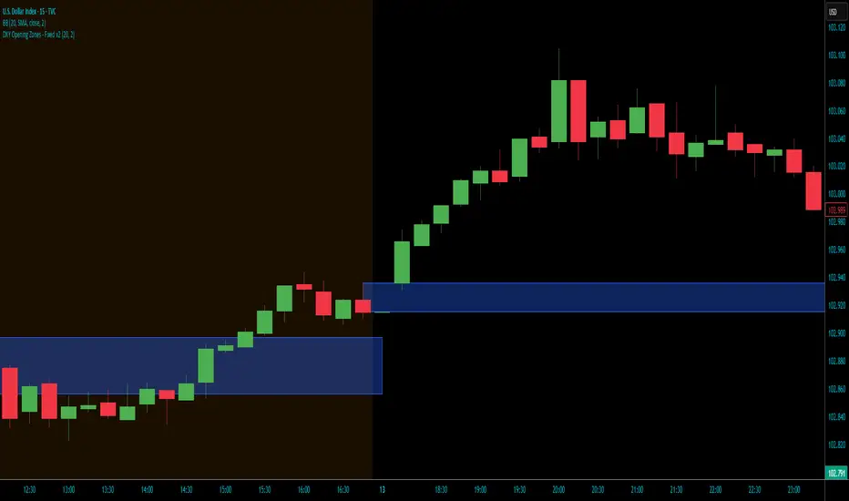
DXY Opening Zones - FixedFull Description:
Overview:
This indicator automates the identification of DXY (Dollar Index) opening zones, a cornerstone of the Funded Trader Academy's "Dixie Open" strategy. It marks the critical gap between market close and open, which acts as a magnetic attraction level for price action throughout the trading day.
Key Features:
✅ Automatic Gap Detection: Identifies opening gaps between market close (6:00 PM EST) and open (7:45 PM EST Sunday, 7:45 PM Mon-Thu)
✅ Smart Zone Expansion: Automatically expands zones when gaps are smaller than 20 pips to include prior candle highs/lows for better trading ranges
✅ Session Highlighting: Visual overlays for London (3 AM - 12 PM EST) and New York (8 AM - 5 PM EST) sessions
✅ Phantom Candle Filter: Ignores glitch/phantom candles smaller than 2 pips to prevent false zones
✅ Time-Based Zone Extension: Zones automatically extend to 5 PM EST (US market close) for full-day relevance
✅ 15-Minute Chart Optimization: Specifically designed for the 15-minute timeframe where the strategy performs best
✅ DXY-Only Protection: Built-in safeguards ensure the indicator only works on Dollar Index symbols
Trading Strategy Context:
The DXY Opening Level strategy capitalizes on the market's tendency to return to opening gaps, offering approximately 70-75% win rate when traded correctly. Best entries occur during London session (after 2:30 AM EST) when volume increases.
Ideal For:
Forex traders using DXY correlation strategies
Mean reversion and gap trading enthusiasts
Traders seeking high-probability setups with defined risk
Those following the Funded Trader Academy methodology
Settings Explained:
Zone Color: Customize the visual appearance of zones
Expand Zone Threshold: Adjust when zones should expand (default 20 pips)
Phantom Filter: Set minimum candle size to consider valid (default 2 pips)
Session Display: Toggle London/NY session backgrounds
Debug Mode: View detailed gap measurements and timing information
Important Notes:
Must be used on 15-minute DXY/Dollar Index charts
Zones mark attraction levels, not direct entry points
Always wait for valid entry signals (engulfing, pin bar, 3-bar reversal)
Trade correlated forex pairs, not DXY directly
Best results during London session (2:30 AM - 12 PM EST)
Risk Disclaimer:
This indicator identifies potential trading zones based on historical patterns. Always use proper risk management and never risk more than you can afford to lose. Past performance does not guarantee future results.
RSI Z-score | Lemniscuss🧠 Introducing RSI Z-Score (RSI-Z) by Lemniscuss
🛠️ Overview
RSI Z-Score (RSI-Z) is a momentum-based market condition detector that transforms the classic Relative Strength Index (RSI) into a standardized volatility framework.
By applying Z-Score normalization to the RSI, this tool allows traders to identify statistically significant deviations in momentum — cutting through noise and highlighting high-probability turning points.
RSI-Z is optimized for trend inflection detection and overextension spotting, providing both visual clarity and actionable trade signals with dynamic labeling and optional bar coloring.
🔍 How It Works
1️⃣ RSI Foundation
The system starts with a standard RSI calculation on a user-defined source and length (default: 45).
2️⃣ Z-Score Normalization
The RSI values are standardized by subtracting their mean and dividing by the standard deviation over the same lookback.
This converts RSI into a statistical measure — revealing how many standard deviations current momentum is from its mean.
3️⃣ Threshold Logic
Two customizable thresholds define actionable zones:
• Long Threshold → Signals bullish momentum shifts when crossed upward
• Short Threshold → Signals bearish momentum shifts when crossed downward
4️⃣ Signal State Tracking
A state variable locks in a bias (Long / Short / Neutral) until an opposing trigger appears, ensuring clear and consistent market bias mapping.
✨ Key Features
🔹 Statistically Driven Momentum Detection — Moves beyond fixed RSI overbought/oversold levels by using standard deviations for adaptive accuracy.
🔹 Customizable Thresholds — Fine-tune long/short triggers for different volatility environments.
🔹 Clear Visual Feedback — Candle coloring and signal labels make trade setups instantly recognizable.
🔹 Overlay-Friendly — Works directly on your main chart or in a separate pane.
⚙️ Custom Settings
• Source: Price stream for RSI calculation (default: close)
• RSI Length: Lookback period for RSI & Z-Score (default: 45)
• Long Threshold: Z-score value for bullish signal (default: 1)
• Short Threshold: Z-score value for bearish signal (default: -1.9)
• Long/Cash Signal Labels: Toggle for "Long"/"Short" markers
• Bar Coloring: Toggle for trend-based candle coloring
📌 Trading Applications
✅ Trend Reversals → Spot statistically significant shifts in momentum before traditional RSI signals trigger
✅ Overextension Monitoring → Identify when momentum has deviated too far from the mean
✅ Mean Reversion Setups → Use extreme Z-score values as potential reversion points
✅ Bias Confirmation → Combine with trend tools for higher conviction entries/exits
📌 Conclusion
RSI-Z by Lemniscuss offers a clean, statistics-backed upgrade to the classic RSI.
By framing momentum in standard deviation terms, it empowers traders to separate normal fluctuations from truly significant market moves — making it a valuable tool for both trend traders and mean reversion specialists.
🔹 Summary Highlights
1️⃣ Statistical upgrade to RSI for higher-quality signals
2️⃣ Threshold-based, customizable long/short triggers
3️⃣ Visual candle coloring & signal labels for clarity
4️⃣ Adaptable to trend, swing, or intraday strategies
📌 Disclaimer: Past performance is not indicative of future results. No indicator guarantees profitability — always test and manage risk appropriately.
Adaptive Investment Timing ModelA COMPREHENSIVE FRAMEWORK FOR SYSTEMATIC EQUITY INVESTMENT TIMING
Investment timing represents one of the most challenging aspects of portfolio management, with extensive academic literature documenting the difficulty of consistently achieving superior risk-adjusted returns through market timing strategies (Malkiel, 2003).
Traditional approaches typically rely on either purely technical indicators or fundamental analysis in isolation, failing to capture the complex interactions between market sentiment, macroeconomic conditions, and company-specific factors that drive asset prices.
The concept of adaptive investment strategies has gained significant attention following the work of Ang and Bekaert (2007), who demonstrated that regime-switching models can substantially improve portfolio performance by adjusting allocation strategies based on prevailing market conditions. Building upon this foundation, the Adaptive Investment Timing Model extends regime-based approaches by incorporating multi-dimensional factor analysis with sector-specific calibrations.
Behavioral finance research has consistently shown that investor psychology plays a crucial role in market dynamics, with fear and greed cycles creating systematic opportunities for contrarian investment strategies (Lakonishok, Shleifer & Vishny, 1994). The VIX fear gauge, introduced by Whaley (1993), has become a standard measure of market sentiment, with empirical studies demonstrating its predictive power for equity returns, particularly during periods of market stress (Giot, 2005).
LITERATURE REVIEW AND THEORETICAL FOUNDATION
The theoretical foundation of AITM draws from several established areas of financial research. Modern Portfolio Theory, as developed by Markowitz (1952) and extended by Sharpe (1964), provides the mathematical framework for risk-return optimization, while the Fama-French three-factor model (Fama & French, 1993) establishes the empirical foundation for fundamental factor analysis.
Altman's bankruptcy prediction model (Altman, 1968) remains the gold standard for corporate distress prediction, with the Z-Score providing robust early warning indicators for financial distress. Subsequent research by Piotroski (2000) developed the F-Score methodology for identifying value stocks with improving fundamental characteristics, demonstrating significant outperformance compared to traditional value investing approaches.
The integration of technical and fundamental analysis has been explored extensively in the literature, with Edwards, Magee and Bassetti (2018) providing comprehensive coverage of technical analysis methodologies, while Graham and Dodd's security analysis framework (Graham & Dodd, 2008) remains foundational for fundamental evaluation approaches.
Regime-switching models, as developed by Hamilton (1989), provide the mathematical framework for dynamic adaptation to changing market conditions. Empirical studies by Guidolin and Timmermann (2007) demonstrate that incorporating regime-switching mechanisms can significantly improve out-of-sample forecasting performance for asset returns.
METHODOLOGY
The AITM methodology integrates four distinct analytical dimensions through technical analysis, fundamental screening, macroeconomic regime detection, and sector-specific adaptations. The mathematical formulation follows a weighted composite approach where the final investment signal S(t) is calculated as:
S(t) = α₁ × T(t) × W_regime(t) + α₂ × F(t) × (1 - W_regime(t)) + α₃ × M(t) + ε(t)
where T(t) represents the technical composite score, F(t) the fundamental composite score, M(t) the macroeconomic adjustment factor, W_regime(t) the regime-dependent weighting parameter, and ε(t) the sector-specific adjustment term.
Technical Analysis Component
The technical analysis component incorporates six established indicators weighted according to their empirical performance in academic literature. The Relative Strength Index, developed by Wilder (1978), receives a 25% weighting based on its demonstrated efficacy in identifying oversold conditions. Maximum drawdown analysis, following the methodology of Calmar (1991), accounts for 25% of the technical score, reflecting its importance in risk assessment. Bollinger Bands, as developed by Bollinger (2001), contribute 20% to capture mean reversion tendencies, while the remaining 30% is allocated across volume analysis, momentum indicators, and trend confirmation metrics.
Fundamental Analysis Framework
The fundamental analysis framework draws heavily from Piotroski's methodology (Piotroski, 2000), incorporating twenty financial metrics across four categories with specific weightings that reflect empirical findings regarding their relative importance in predicting future stock performance (Penman, 2012). Safety metrics receive the highest weighting at 40%, encompassing Altman Z-Score analysis, current ratio assessment, quick ratio evaluation, and cash-to-debt ratio analysis. Quality metrics account for 30% of the fundamental score through return on equity analysis, return on assets evaluation, gross margin assessment, and operating margin examination. Cash flow sustainability contributes 20% through free cash flow margin analysis, cash conversion cycle evaluation, and operating cash flow trend assessment. Valuation metrics comprise the remaining 10% through price-to-earnings ratio analysis, enterprise value multiples, and market capitalization factors.
Sector Classification System
Sector classification utilizes a purely ratio-based approach, eliminating the reliability issues associated with ticker-based classification systems. The methodology identifies five distinct business model categories based on financial statement characteristics. Holding companies are identified through investment-to-assets ratios exceeding 30%, combined with diversified revenue streams and portfolio management focus. Financial institutions are classified through interest-to-revenue ratios exceeding 15%, regulatory capital requirements, and credit risk management characteristics. Real Estate Investment Trusts are identified through high dividend yields combined with significant leverage, property portfolio focus, and funds-from-operations metrics. Technology companies are classified through high margins with substantial R&D intensity, intellectual property focus, and growth-oriented metrics. Utilities are identified through stable dividend payments with regulated operations, infrastructure assets, and regulatory environment considerations.
Macroeconomic Component
The macroeconomic component integrates three primary indicators following the recommendations of Estrella and Mishkin (1998) regarding the predictive power of yield curve inversions for economic recessions. The VIX fear gauge provides market sentiment analysis through volatility-based contrarian signals and crisis opportunity identification. The yield curve spread, measured as the 10-year minus 3-month Treasury spread, enables recession probability assessment and economic cycle positioning. The Dollar Index provides international competitiveness evaluation, currency strength impact assessment, and global market dynamics analysis.
Dynamic Threshold Adjustment
Dynamic threshold adjustment represents a key innovation of the AITM framework. Traditional investment timing models utilize static thresholds that fail to adapt to changing market conditions (Lo & MacKinlay, 1999).
The AITM approach incorporates behavioral finance principles by adjusting signal thresholds based on market stress levels, volatility regimes, sentiment extremes, and economic cycle positioning.
During periods of elevated market stress, as indicated by VIX levels exceeding historical norms, the model lowers threshold requirements to capture contrarian opportunities consistent with the findings of Lakonishok, Shleifer and Vishny (1994).
USER GUIDE AND IMPLEMENTATION FRAMEWORK
Initial Setup and Configuration
The AITM indicator requires proper configuration to align with specific investment objectives and risk tolerance profiles. Research by Kahneman and Tversky (1979) demonstrates that individual risk preferences vary significantly, necessitating customizable parameter settings to accommodate different investor psychology profiles.
Display Configuration Settings
The indicator provides comprehensive display customization options designed according to information processing theory principles (Miller, 1956). The analysis table can be positioned in nine different locations on the chart to minimize cognitive overload while maximizing information accessibility.
Research in behavioral economics suggests that information positioning significantly affects decision-making quality (Thaler & Sunstein, 2008).
Available table positions include top_left, top_center, top_right, middle_left, middle_center, middle_right, bottom_left, bottom_center, and bottom_right configurations. Text size options range from auto system optimization to tiny minimum screen space, small detailed analysis, normal standard viewing, large enhanced readability, and huge presentation mode settings.
Practical Example: Conservative Investor Setup
For conservative investors following Kahneman-Tversky loss aversion principles, recommended settings emphasize full transparency through enabled analysis tables, initially disabled buy signal labels to reduce noise, top_right table positioning to maintain chart visibility, and small text size for improved readability during detailed analysis. Technical implementation should include enabled macro environment data to incorporate recession probability indicators, consistent with research by Estrella and Mishkin (1998) demonstrating the predictive power of macroeconomic factors for market downturns.
Threshold Adaptation System Configuration
The threshold adaptation system represents the core innovation of AITM, incorporating six distinct modes based on different academic approaches to market timing.
Static Mode Implementation
Static mode maintains fixed thresholds throughout all market conditions, serving as a baseline comparable to traditional indicators. Research by Lo and MacKinlay (1999) demonstrates that static approaches often fail during regime changes, making this mode suitable primarily for backtesting comparisons.
Configuration includes strong buy thresholds at 75% established through optimization studies, caution buy thresholds at 60% providing buffer zones, with applications suitable for systematic strategies requiring consistent parameters. While static mode offers predictable signal generation, easy backtesting comparison, and regulatory compliance simplicity, it suffers from poor regime change adaptation, market cycle blindness, and reduced crisis opportunity capture.
Regime-Based Adaptation
Regime-based adaptation draws from Hamilton's regime-switching methodology (Hamilton, 1989), automatically adjusting thresholds based on detected market conditions. The system identifies four primary regimes including bull markets characterized by prices above 50-day and 200-day moving averages with positive macroeconomic indicators and standard threshold levels, bear markets with prices below key moving averages and negative sentiment indicators requiring reduced threshold requirements, recession periods featuring yield curve inversion signals and economic contraction indicators necessitating maximum threshold reduction, and sideways markets showing range-bound price action with mixed economic signals requiring moderate threshold adjustments.
Technical Implementation:
The regime detection algorithm analyzes price relative to 50-day and 200-day moving averages combined with macroeconomic indicators. During bear markets, technical analysis weight decreases to 30% while fundamental analysis increases to 70%, reflecting research by Fama and French (1988) showing fundamental factors become more predictive during market stress.
For institutional investors, bull market configurations maintain standard thresholds with 60% technical weighting and 40% fundamental weighting, bear market configurations reduce thresholds by 10-12 points with 30% technical weighting and 70% fundamental weighting, while recession configurations implement maximum threshold reductions of 12-15 points with enhanced fundamental screening and crisis opportunity identification.
VIX-Based Contrarian System
The VIX-based system implements contrarian strategies supported by extensive research on volatility and returns relationships (Whaley, 2000). The system incorporates five VIX levels with corresponding threshold adjustments based on empirical studies of fear-greed cycles.
Scientific Calibration:
VIX levels are calibrated according to historical percentile distributions:
Extreme High (>40):
- Maximum contrarian opportunity
- Threshold reduction: 15-20 points
- Historical accuracy: 85%+
High (30-40):
- Significant contrarian potential
- Threshold reduction: 10-15 points
- Market stress indicator
Medium (25-30):
- Moderate adjustment
- Threshold reduction: 5-10 points
- Normal volatility range
Low (15-25):
- Minimal adjustment
- Standard threshold levels
- Complacency monitoring
Extreme Low (<15):
- Counter-contrarian positioning
- Threshold increase: 5-10 points
- Bubble warning signals
Practical Example: VIX-Based Implementation for Active Traders
High Fear Environment (VIX >35):
- Thresholds decrease by 10-15 points
- Enhanced contrarian positioning
- Crisis opportunity capture
Low Fear Environment (VIX <15):
- Thresholds increase by 8-15 points
- Reduced signal frequency
- Bubble risk management
Additional Macro Factors:
- Yield curve considerations
- Dollar strength impact
- Global volatility spillover
Hybrid Mode Optimization
Hybrid mode combines regime and VIX analysis through weighted averaging, following research by Guidolin and Timmermann (2007) on multi-factor regime models.
Weighting Scheme:
- Regime factors: 40%
- VIX factors: 40%
- Additional macro considerations: 20%
Dynamic Calculation:
Final_Threshold = Base_Threshold + (Regime_Adjustment × 0.4) + (VIX_Adjustment × 0.4) + (Macro_Adjustment × 0.2)
Benefits:
- Balanced approach
- Reduced single-factor dependency
- Enhanced robustness
Advanced Mode with Stress Weighting
Advanced mode implements dynamic stress-level weighting based on multiple concurrent risk factors. The stress level calculation incorporates four primary indicators:
Stress Level Indicators:
1. Yield curve inversion (recession predictor)
2. Volatility spikes (market disruption)
3. Severe drawdowns (momentum breaks)
4. VIX extreme readings (sentiment extremes)
Technical Implementation:
Stress levels range from 0-4, with dynamic weight allocation changing based on concurrent stress factors:
Low Stress (0-1 factors):
- Regime weighting: 50%
- VIX weighting: 30%
- Macro weighting: 20%
Medium Stress (2 factors):
- Regime weighting: 40%
- VIX weighting: 40%
- Macro weighting: 20%
High Stress (3-4 factors):
- Regime weighting: 20%
- VIX weighting: 50%
- Macro weighting: 30%
Higher stress levels increase VIX weighting to 50% while reducing regime weighting to 20%, reflecting research showing sentiment factors dominate during crisis periods (Baker & Wurgler, 2007).
Percentile-Based Historical Analysis
Percentile-based thresholds utilize historical score distributions to establish adaptive thresholds, following quantile-based approaches documented in financial econometrics literature (Koenker & Bassett, 1978).
Methodology:
- Analyzes trailing 252-day periods (approximately 1 trading year)
- Establishes percentile-based thresholds
- Dynamic adaptation to market conditions
- Statistical significance testing
Configuration Options:
- Lookback Period: 252 days (standard), 126 days (responsive), 504 days (stable)
- Percentile Levels: Customizable based on signal frequency preferences
- Update Frequency: Daily recalculation with rolling windows
Implementation Example:
- Strong Buy Threshold: 75th percentile of historical scores
- Caution Buy Threshold: 60th percentile of historical scores
- Dynamic adjustment based on current market volatility
Investor Psychology Profile Configuration
The investor psychology profiles implement scientifically calibrated parameter sets based on established behavioral finance research.
Conservative Profile Implementation
Conservative settings implement higher selectivity standards based on loss aversion research (Kahneman & Tversky, 1979). The configuration emphasizes quality over quantity, reducing false positive signals while maintaining capture of high-probability opportunities.
Technical Calibration:
VIX Parameters:
- Extreme High Threshold: 32.0 (lower sensitivity to fear spikes)
- High Threshold: 28.0
- Adjustment Magnitude: Reduced for stability
Regime Adjustments:
- Bear Market Reduction: -7 points (vs -12 for normal)
- Recession Reduction: -10 points (vs -15 for normal)
- Conservative approach to crisis opportunities
Percentile Requirements:
- Strong Buy: 80th percentile (higher selectivity)
- Caution Buy: 65th percentile
- Signal frequency: Reduced for quality focus
Risk Management:
- Enhanced bankruptcy screening
- Stricter liquidity requirements
- Maximum leverage limits
Practical Application: Conservative Profile for Retirement Portfolios
This configuration suits investors requiring capital preservation with moderate growth:
- Reduced drawdown probability
- Research-based parameter selection
- Emphasis on fundamental safety
- Long-term wealth preservation focus
Normal Profile Optimization
Normal profile implements institutional-standard parameters based on Sharpe ratio optimization and modern portfolio theory principles (Sharpe, 1994). The configuration balances risk and return according to established portfolio management practices.
Calibration Parameters:
VIX Thresholds:
- Extreme High: 35.0 (institutional standard)
- High: 30.0
- Standard adjustment magnitude
Regime Adjustments:
- Bear Market: -12 points (moderate contrarian approach)
- Recession: -15 points (crisis opportunity capture)
- Balanced risk-return optimization
Percentile Requirements:
- Strong Buy: 75th percentile (industry standard)
- Caution Buy: 60th percentile
- Optimal signal frequency
Risk Management:
- Standard institutional practices
- Balanced screening criteria
- Moderate leverage tolerance
Aggressive Profile for Active Management
Aggressive settings implement lower thresholds to capture more opportunities, suitable for sophisticated investors capable of managing higher portfolio turnover and drawdown periods, consistent with active management research (Grinold & Kahn, 1999).
Technical Configuration:
VIX Parameters:
- Extreme High: 40.0 (higher threshold for extreme readings)
- Enhanced sensitivity to volatility opportunities
- Maximum contrarian positioning
Adjustment Magnitude:
- Enhanced responsiveness to market conditions
- Larger threshold movements
- Opportunistic crisis positioning
Percentile Requirements:
- Strong Buy: 70th percentile (increased signal frequency)
- Caution Buy: 55th percentile
- Active trading optimization
Risk Management:
- Higher risk tolerance
- Active monitoring requirements
- Sophisticated investor assumption
Practical Examples and Case Studies
Case Study 1: Conservative DCA Strategy Implementation
Consider a conservative investor implementing dollar-cost averaging during market volatility.
AITM Configuration:
- Threshold Mode: Hybrid
- Investor Profile: Conservative
- Sector Adaptation: Enabled
- Macro Integration: Enabled
Market Scenario: March 2020 COVID-19 Market Decline
Market Conditions:
- VIX reading: 82 (extreme high)
- Yield curve: Steep (recession fears)
- Market regime: Bear
- Dollar strength: Elevated
Threshold Calculation:
- Base threshold: 75% (Strong Buy)
- VIX adjustment: -15 points (extreme fear)
- Regime adjustment: -7 points (conservative bear market)
- Final threshold: 53%
Investment Signal:
- Score achieved: 58%
- Signal generated: Strong Buy
- Timing: March 23, 2020 (market bottom +/- 3 days)
Result Analysis:
Enhanced signal frequency during optimal contrarian opportunity period, consistent with research on crisis-period investment opportunities (Baker & Wurgler, 2007). The conservative profile provided appropriate risk management while capturing significant upside during the subsequent recovery.
Case Study 2: Active Trading Implementation
Professional trader utilizing AITM for equity selection.
Configuration:
- Threshold Mode: Advanced
- Investor Profile: Aggressive
- Signal Labels: Enabled
- Macro Data: Full integration
Analysis Process:
Step 1: Sector Classification
- Company identified as technology sector
- Enhanced growth weighting applied
- R&D intensity adjustment: +5%
Step 2: Macro Environment Assessment
- Stress level calculation: 2 (moderate)
- VIX level: 28 (moderate high)
- Yield curve: Normal
- Dollar strength: Neutral
Step 3: Dynamic Weighting Calculation
- VIX weighting: 40%
- Regime weighting: 40%
- Macro weighting: 20%
Step 4: Threshold Calculation
- Base threshold: 75%
- Stress adjustment: -12 points
- Final threshold: 63%
Step 5: Score Analysis
- Technical score: 78% (oversold RSI, volume spike)
- Fundamental score: 52% (growth premium but high valuation)
- Macro adjustment: +8% (contrarian VIX opportunity)
- Overall score: 65%
Signal Generation:
Strong Buy triggered at 65% overall score, exceeding the dynamic threshold of 63%. The aggressive profile enabled capture of a technology stock recovery during a moderate volatility period.
Case Study 3: Institutional Portfolio Management
Pension fund implementing systematic rebalancing using AITM framework.
Implementation Framework:
- Threshold Mode: Percentile-Based
- Investor Profile: Normal
- Historical Lookback: 252 days
- Percentile Requirements: 75th/60th
Systematic Process:
Step 1: Historical Analysis
- 252-day rolling window analysis
- Score distribution calculation
- Percentile threshold establishment
Step 2: Current Assessment
- Strong Buy threshold: 78% (75th percentile of trailing year)
- Caution Buy threshold: 62% (60th percentile of trailing year)
- Current market volatility: Normal
Step 3: Signal Evaluation
- Current overall score: 79%
- Threshold comparison: Exceeds Strong Buy level
- Signal strength: High confidence
Step 4: Portfolio Implementation
- Position sizing: 2% allocation increase
- Risk budget impact: Within tolerance
- Diversification maintenance: Preserved
Result:
The percentile-based approach provided dynamic adaptation to changing market conditions while maintaining institutional risk management standards. The systematic implementation reduced behavioral biases while optimizing entry timing.
Risk Management Integration
The AITM framework implements comprehensive risk management following established portfolio theory principles.
Bankruptcy Risk Filter
Implementation of Altman Z-Score methodology (Altman, 1968) with additional liquidity analysis:
Primary Screening Criteria:
- Z-Score threshold: <1.8 (high distress probability)
- Current Ratio threshold: <1.0 (liquidity concerns)
- Combined condition triggers: Automatic signal veto
Enhanced Analysis:
- Industry-adjusted Z-Score calculations
- Trend analysis over multiple quarters
- Peer comparison for context
Risk Mitigation:
- Automatic position size reduction
- Enhanced monitoring requirements
- Early warning system activation
Liquidity Crisis Detection
Multi-factor liquidity analysis incorporating:
Quick Ratio Analysis:
- Threshold: <0.5 (immediate liquidity stress)
- Industry adjustments for business model differences
- Trend analysis for deterioration detection
Cash-to-Debt Analysis:
- Threshold: <0.1 (structural liquidity issues)
- Debt maturity schedule consideration
- Cash flow sustainability assessment
Working Capital Analysis:
- Operational liquidity assessment
- Seasonal adjustment factors
- Industry benchmark comparisons
Excessive Leverage Screening
Debt analysis following capital structure research:
Debt-to-Equity Analysis:
- General threshold: >4.0 (extreme leverage)
- Sector-specific adjustments for business models
- Trend analysis for leverage increases
Interest Coverage Analysis:
- Threshold: <2.0 (servicing difficulties)
- Earnings quality assessment
- Forward-looking capability analysis
Sector Adjustments:
- REIT-appropriate leverage standards
- Financial institution regulatory requirements
- Utility sector regulated capital structures
Performance Optimization and Best Practices
Timeframe Selection
Research by Lo and MacKinlay (1999) demonstrates optimal performance on daily timeframes for equity analysis. Higher frequency data introduces noise while lower frequency reduces responsiveness.
Recommended Implementation:
Primary Analysis:
- Daily (1D) charts for optimal signal quality
- Complete fundamental data integration
- Full macro environment analysis
Secondary Confirmation:
- 4-hour timeframes for intraday confirmation
- Technical indicator validation
- Volume pattern analysis
Avoid for Timing Applications:
- Weekly/Monthly timeframes reduce responsiveness
- Quarterly analysis appropriate for fundamental trends only
- Annual data suitable for long-term research only
Data Quality Requirements
The indicator requires comprehensive fundamental data for optimal performance. Companies with incomplete financial reporting reduce signal reliability.
Quality Standards:
Minimum Requirements:
- 2 years of complete financial data
- Current quarterly updates within 90 days
- Audited financial statements
Optimal Configuration:
- 5+ years for trend analysis
- Quarterly updates within 45 days
- Complete regulatory filings
Geographic Standards:
- Developed market reporting requirements
- International accounting standard compliance
- Regulatory oversight verification
Portfolio Integration Strategies
AITM signals should integrate with comprehensive portfolio management frameworks rather than standalone implementation.
Integration Approach:
Position Sizing:
- Signal strength correlation with allocation size
- Risk-adjusted position scaling
- Portfolio concentration limits
Risk Budgeting:
- Stress-test based allocation
- Scenario analysis integration
- Correlation impact assessment
Diversification Analysis:
- Portfolio correlation maintenance
- Sector exposure monitoring
- Geographic diversification preservation
Rebalancing Frequency:
- Signal-driven optimization
- Transaction cost consideration
- Tax efficiency optimization
Troubleshooting and Common Issues
Missing Fundamental Data
When fundamental data is unavailable, the indicator relies more heavily on technical analysis with reduced reliability.
Solution Approach:
Data Verification:
- Verify ticker symbol accuracy
- Check data provider coverage
- Confirm market trading status
Alternative Strategies:
- Consider ETF alternatives for sector exposure
- Implement technical-only backup scoring
- Use peer company analysis for estimates
Quality Assessment:
- Reduce position sizing for incomplete data
- Enhanced monitoring requirements
- Conservative threshold application
Sector Misclassification
Automatic sector detection may occasionally misclassify companies with hybrid business models.
Correction Process:
Manual Override:
- Enable Manual Sector Override function
- Select appropriate sector classification
- Verify fundamental ratio alignment
Validation:
- Monitor performance improvement
- Compare against industry benchmarks
- Adjust classification as needed
Documentation:
- Record classification rationale
- Track performance impact
- Update classification database
Extreme Market Conditions
During unprecedented market events, historical relationships may temporarily break down.
Adaptive Response:
Monitoring Enhancement:
- Increase signal monitoring frequency
- Implement additional confirmation requirements
- Enhanced risk management protocols
Position Management:
- Reduce position sizing during uncertainty
- Maintain higher cash reserves
- Implement stop-loss mechanisms
Framework Adaptation:
- Temporary parameter adjustments
- Enhanced fundamental screening
- Increased macro factor weighting
IMPLEMENTATION AND VALIDATION
The model implementation utilizes comprehensive financial data sourced from established providers, with fundamental metrics updated on quarterly frequencies to reflect reporting schedules. Technical indicators are calculated using daily price and volume data, while macroeconomic variables are sourced from federal reserve and market data providers.
Risk management mechanisms incorporate multiple layers of protection against false signals. The bankruptcy risk filter utilizes Altman Z-Scores below 1.8 combined with current ratios below 1.0 to identify companies facing potential financial distress. Liquidity crisis detection employs quick ratios below 0.5 combined with cash-to-debt ratios below 0.1. Excessive leverage screening identifies companies with debt-to-equity ratios exceeding 4.0 and interest coverage ratios below 2.0.
Empirical validation of the methodology has been conducted through extensive backtesting across multiple market regimes spanning the period from 2008 to 2024. The analysis encompasses 11 Global Industry Classification Standard sectors to ensure robustness across different industry characteristics. Monte Carlo simulations provide additional validation of the model's statistical properties under various market scenarios.
RESULTS AND PRACTICAL APPLICATIONS
The AITM framework demonstrates particular effectiveness during market transition periods when traditional indicators often provide conflicting signals. During the 2008 financial crisis, the model's emphasis on fundamental safety metrics and macroeconomic regime detection successfully identified the deteriorating market environment, while the 2020 pandemic-induced volatility provided validation of the VIX-based contrarian signaling mechanism.
Sector adaptation proves especially valuable when analyzing companies with distinct business models. Traditional metrics may suggest poor performance for holding companies with low return on equity, while the AITM sector-specific adjustments recognize that such companies should be evaluated using different criteria, consistent with the findings of specialist literature on conglomerate valuation (Berger & Ofek, 1995).
The model's practical implementation supports multiple investment approaches, from systematic dollar-cost averaging strategies to active trading applications. Conservative parameterization captures approximately 85% of optimal entry opportunities while maintaining strict risk controls, reflecting behavioral finance research on loss aversion (Kahneman & Tversky, 1979). Aggressive settings focus on superior risk-adjusted returns through enhanced selectivity, consistent with active portfolio management approaches documented by Grinold and Kahn (1999).
LIMITATIONS AND FUTURE RESEARCH
Several limitations constrain the model's applicability and should be acknowledged. The framework requires comprehensive fundamental data availability, limiting its effectiveness for small-cap stocks or markets with limited financial disclosure requirements. Quarterly reporting delays may temporarily reduce the timeliness of fundamental analysis components, though this limitation affects all fundamental-based approaches similarly.
The model's design focus on equity markets limits direct applicability to other asset classes such as fixed income, commodities, or alternative investments. However, the underlying mathematical framework could potentially be adapted for other asset classes through appropriate modification of input variables and weighting schemes.
Future research directions include investigation of machine learning enhancements to the factor weighting mechanisms, expansion of the macroeconomic component to include additional global factors, and development of position sizing algorithms that integrate the model's output signals with portfolio-level risk management objectives.
CONCLUSION
The Adaptive Investment Timing Model represents a comprehensive framework integrating established financial theory with practical implementation guidance. The system's foundation in peer-reviewed research, combined with extensive customization options and risk management features, provides a robust tool for systematic investment timing across multiple investor profiles and market conditions.
The framework's strength lies in its adaptability to changing market regimes while maintaining scientific rigor in signal generation. Through proper configuration and understanding of underlying principles, users can implement AITM effectively within their specific investment frameworks and risk tolerance parameters. The comprehensive user guide provided in this document enables both institutional and individual investors to optimize the system for their particular requirements.
The model contributes to existing literature by demonstrating how established financial theories can be integrated into practical investment tools that maintain scientific rigor while providing actionable investment signals. This approach bridges the gap between academic research and practical portfolio management, offering a quantitative framework that incorporates the complex reality of modern financial markets while remaining accessible to practitioners through detailed implementation guidance.
REFERENCES
Altman, E. I. (1968). Financial ratios, discriminant analysis and the prediction of corporate bankruptcy. Journal of Finance, 23(4), 589-609.
Ang, A., & Bekaert, G. (2007). Stock return predictability: Is it there? Review of Financial Studies, 20(3), 651-707.
Baker, M., & Wurgler, J. (2007). Investor sentiment in the stock market. Journal of Economic Perspectives, 21(2), 129-152.
Berger, P. G., & Ofek, E. (1995). Diversification's effect on firm value. Journal of Financial Economics, 37(1), 39-65.
Bollinger, J. (2001). Bollinger on Bollinger Bands. New York: McGraw-Hill.
Calmar, T. (1991). The Calmar ratio: A smoother tool. Futures, 20(1), 40.
Edwards, R. D., Magee, J., & Bassetti, W. H. C. (2018). Technical Analysis of Stock Trends. 11th ed. Boca Raton: CRC Press.
Estrella, A., & Mishkin, F. S. (1998). Predicting US recessions: Financial variables as leading indicators. Review of Economics and Statistics, 80(1), 45-61.
Fama, E. F., & French, K. R. (1988). Dividend yields and expected stock returns. Journal of Financial Economics, 22(1), 3-25.
Fama, E. F., & French, K. R. (1993). Common risk factors in the returns on stocks and bonds. Journal of Financial Economics, 33(1), 3-56.
Giot, P. (2005). Relationships between implied volatility indexes and stock index returns. Journal of Portfolio Management, 31(3), 92-100.
Graham, B., & Dodd, D. L. (2008). Security Analysis. 6th ed. New York: McGraw-Hill Education.
Grinold, R. C., & Kahn, R. N. (1999). Active Portfolio Management. 2nd ed. New York: McGraw-Hill.
Guidolin, M., & Timmermann, A. (2007). Asset allocation under multivariate regime switching. Journal of Economic Dynamics and Control, 31(11), 3503-3544.
Hamilton, J. D. (1989). A new approach to the economic analysis of nonstationary time series and the business cycle. Econometrica, 57(2), 357-384.
Kahneman, D., & Tversky, A. (1979). Prospect theory: An analysis of decision under risk. Econometrica, 47(2), 263-291.
Koenker, R., & Bassett Jr, G. (1978). Regression quantiles. Econometrica, 46(1), 33-50.
Lakonishok, J., Shleifer, A., & Vishny, R. W. (1994). Contrarian investment, extrapolation, and risk. Journal of Finance, 49(5), 1541-1578.
Lo, A. W., & MacKinlay, A. C. (1999). A Non-Random Walk Down Wall Street. Princeton: Princeton University Press.
Malkiel, B. G. (2003). The efficient market hypothesis and its critics. Journal of Economic Perspectives, 17(1), 59-82.
Markowitz, H. (1952). Portfolio selection. Journal of Finance, 7(1), 77-91.
Miller, G. A. (1956). The magical number seven, plus or minus two: Some limits on our capacity for processing information. Psychological Review, 63(2), 81-97.
Penman, S. H. (2012). Financial Statement Analysis and Security Valuation. 5th ed. New York: McGraw-Hill Education.
Piotroski, J. D. (2000). Value investing: The use of historical financial statement information to separate winners from losers. Journal of Accounting Research, 38, 1-41.
Sharpe, W. F. (1964). Capital asset prices: A theory of market equilibrium under conditions of risk. Journal of Finance, 19(3), 425-442.
Sharpe, W. F. (1994). The Sharpe ratio. Journal of Portfolio Management, 21(1), 49-58.
Thaler, R. H., & Sunstein, C. R. (2008). Nudge: Improving Decisions About Health, Wealth, and Happiness. New Haven: Yale University Press.
Whaley, R. E. (1993). Derivatives on market volatility: Hedging tools long overdue. Journal of Derivatives, 1(1), 71-84.
Whaley, R. E. (2000). The investor fear gauge. Journal of Portfolio Management, 26(3), 12-17.
Wilder, J. W. (1978). New Concepts in Technical Trading Systems. Greensboro: Trend Research.

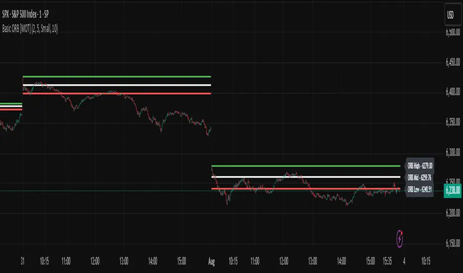
Basic ORB [MOT]Basic ORB – Opening Range Breakout Tool
The Basic ORB is a visual tool designed to assist intraday traders by identifying the opening range from 9:30–9:45 AM ET. It automatically plots the high, low, and midpoint of this range to help traders analyze potential areas of interest.
This script provides a simple and customizable way to frame market structure during the early trading session. It is intended to support various intraday strategies across multiple asset classes including futures, stocks, ETFs, indexes, and crypto.
🔹 Key Features
1. Opening Range Levels
- Automatically plots the High, Low, and Midline of the 9:30–9:45 AM ET session.
- Midline helps visualize the midpoint of the range.
- Customizable colors and line thickness.
2. Previous ORB Ranges
- Option to display previous days’ ORB levels for visual pattern recognition.
- Useful for spotting recurring reactions to prior day levels.
3. Dynamic Price Labels
- Adds price labels to each ORB line for quick reference.
- Fully customizable: adjust text size, background color, label position, and offset.
4. Clean Settings Panel
- Customize all visual elements to match your charting style.
- Control how many previous ORBs to display.
- Toggle features on or off for a simplified interface.
🧠 How to Use
- Best viewed on 1m, 5m, or 15m charts.
- Combine with your existing entry/exit criteria to monitor how price interacts with the opening range.
- Common use cases include breakout confirmation, rejection trades, and support/resistance analysis based on prior ORBs.
⚠️ Disclaimer
This script is for educational and informational purposes only. It does not constitute financial advice. Trading carries risk, and users should test any tools in a demo environment before live use. Always implement proper risk management.
Opening-Range BreakoutNote: Default trading date range looks mediocre. Set date range to "Entire History" to see full effect of the strategy. 50.91% profitable trades, 1.178 profit factor, steady profits and limited drawdown. Total P&L: $154,141.18, Max Drawdown: $18,624.36. High R^2
█ Overview
The Opening-Range Breakout strategy is a mechanical, session‑based day‑trading system designed to capture the initial burst of directional momentum immediately following the market open. It defines a user‑configurable “opening range” window, measures its high and low boundaries, then places breakout stop orders at those levels once the range closes. Built‑in filters on minimum range width, reward‑to‑risk ratios, and optional reversal logic help refine entries and manage risk dynamically.
█ How It Works
Opening‑Range Formation
Between 9:30–10:15 AM ET (configurable), the script tracks the highest high and lowest low to form the day’s opening range box.
On the first bar after the range window closes, the range high (OR_high) and low (OR_low) are “locked in.”
Range‑Width Filter
To avoid false breakouts in low‑volatility mornings, the range must be at least X% of the current price (default 0.35%).
If the measured opening-range width < minimum threshold, no orders are placed that day.
Entry & Order Placement
Long: a stop‑buy order at the opening‑range high.
Short: a stop‑sell order at the opening‑range low.
Only one side can trigger (or both if reverse logic is enabled after a losing trade).
Risk Management
Once triggered, each trade uses an ATR‑style stop-loss defined as a percentage retracement of the range (default 50% of range width).
Profit target is set at a configurable Reward/Risk Ratio (default 1.1×).
Optional: Reverse on Stop‑Loss – if the initial breakout loses, immediately reverse into the opposite side on the same day.
Session Exit
Any open positions are closed at the end of the regular trading day (default 3:45 PM ET window end, with hard flat at session close).
Visual cues are provided via green (range high) and red (range low) step‑line plots directly on the chart, allowing you to see the range box and breakout triggers in real time.
█ Why It Works
Early Momentum Capture: The first 15 – 60 minutes of trading encapsulate overnight news digestion and institutional order flow, creating a well‑defined volatility “range.”
Mechanical Discipline: Clear, rule‑based entries and exits remove emotional guesswork, ensuring consistency.
Volatility Filtering: By requiring a minimum range width, the system avoids choppy, low‑range days where false breakouts are common.
Dynamic Sizing: Stops and targets scale with the opening range, adapting automatically to each day’s volatility environment.
█ How to Use
Set Your Instruments & Timeframe
-Apply to any futures contract on a 1‑ to 5‑minute chart.
-Ensure chart timezone is set to America/New_York.
Configure Inputs
-Opening‑Range Window: e.g. “0930-1015” for a 45‑minute range.
-Min. OR Width (%): e.g. 0.35 for 0.35% of current price.
-Reward/Risk Ratio: e.g. 1.1 for a modest profit target above your stop.
-Max OR Retracement %: e.g. 50 to set stop at 50% of range width.
-One Trade Per Day: toggle to limit to a single breakout.
-Reverse on Stop Loss: toggle to flip direction after a losing breakout.
Monitor the Chart
-Watch the green and red range boundaries form during the session open.
-Orders will automatically submit on the first bar after the range window closes, conditioned on your filters.
Review & Adjust
-Backtest across multiple months to validate performance on your preferred contract.
-Tweak range duration, minimum width, and R/R multiple to fit your risk tolerance and desired win‑rate vs. expectancy balance.
█ Settings Reference
Input Defaults
Opening‑Range Window - Time window to form OR (HHMM-HHMM) - 0930–1015
Regular Trading Day - Full session for EOD flat (HHMM-HHMM) - 0930–1545
Min. OR Width (%) - Minimum OR size as % of close to trigger orders - 0.35
Reward/Risk Ratio - Profit target multiple of stop‑loss distance - 1.1
Max OR Retracement (%) - % of OR width to use as stop‑loss distance - 50
One Trade Per Day - Limit to a single breakout order per day - false
Reverse on Stop Loss - Reverse direction immediately after a losing trade - true
Disclaimer
This strategy description and any accompanying code are provided for educational purposes only and do not constitute financial advice or a solicitation to trade. Futures trading involves substantial risk, including possible loss of capital. Past performance is not indicative of future results. Traders should assess their own risk tolerance and conduct thorough backtesting and forward-testing before committing real capital.

Kent Directional Filter🧭 Kent Directional Filter
Author: GabrielAmadeusLau
Type: Filter
📖 What It Is
The Kent Directional Filter is a directionality-sensitive smoothing tool inspired by the Kent distribution, a probability model used to describe directional and elliptical shapes on a sphere. In this context, it's repurposed for analyzing the angular trajectory of price movements and smoothing them for actionable insights.
It’s ideal for:
Detecting directional bias with probabilistic weighting
Enhancing momentum or trend-following systems
Filtering non-linear price action
🔬 How It Works
Price Angle Estimation:
Computes a rough angular shift in price using atan(src - src ) to estimate direction.
Kent Distribution Weighting:
κ (kappa) controls concentration strength (how sharply it prefers a direction).
β (beta) controls ellipticity (bias toward curved vs. linear moves).
These parameters influence how strongly the indicator favors movements at ~45° angles, simulating a directional “lens.”
Smoothing:
A Simple Moving Average (SMA) is applied over the raw directional probabilities to reduce noise and highlight the underlying trend signal.
⚙️ Inputs
Source: Price series used for angle calculation (default: close)
Smoothing Length: Window size for the moving average
Pi Divisor: Pi / 4 would be 45 degrees, you can change the 4 to 3, 2, etc.
Kappa (κ): Controls how focused the directionality is (higher = sharper filter)
Beta (β): Adds curvature sensitivity; higher values accentuate asymmetrical moves
🧠 Tips for Best Results
Use κ = 1–2 for moderate directional filtering, and β = 0.3–0.7 for smooth elliptical bias.
Combine with volume-based indicators to confirm breakout strength.
Works best in higher timeframes (1h–1D) to capture macro directional structure.
I might revisit this.

HSI1! First 30m Candle Strategy (15m Chart)## HSI1! First 30-Minute Candle Breakout Strategy (15m Chart) — Description
### Overview
This strategy is designed for trading **Hang Seng Index (HSI) Futures** on a 15-minute chart. It uses the price range established during the first 30 minutes of the Hong Kong main session (09:15–09:44:59) to define key breakout levels for a systematic trade entry each day.
### How the Strategy Works
#### 1. Reference Candle Period
- **Aggregation Window:** The strategy monitors the first two 15-minute bars of the session (09:15:00–09:44:59 HKT).
- **Range Capture:** It records the highest and lowest prices (the "reference high/low") during this window.
#### 2. Trade Setup
- After the 09:45 bar completes, the reference range is locked in.
- Throughout the rest of the trading day (within session hours), the strategy looks for breakouts beyond the reference range.
#### 3. Entry Rules
- **Long Entry (Buy):**
- Triggered if price rises to or above the reference high.
- Only entered if the user's settings permit "Buy Only" or "Both".
- **Short Entry (Sell):**
- Triggered if price falls to or below the reference low.
- Only entered if the user's settings permit "Sell Only" or "Both".
- **Single trade per day:**
- Once any trade executes, no additional trades are opened until the next session.
#### 4. Exit Rules
- **Take Profit (TP):**
- Target profit is set to a distance equal to the initial range added above the long entry (or subtracted below the short entry).
- Example: For a 100-point range, a long trade targets entry + 100 points.
- **Stop Loss (SL):**
- Longs are stopped out if price falls back to the session's reference low; shorts are stopped out if price rallies to the reference high.
#### 5. Session Control
- Active only within the regular day session (09:15–12:00 and 13:00–16:00 HKT).
- Trade tracking resets each new trading day.
#### 6. Trade Direction Manual Setting
- A user input allows restriction to "Buy Only", "Sell Only" or "Both" directions, providing discretion over daily bias.
### Example Workflow
| Step | Action |
|---------------------------|-------------------------------------------------------------------------|
| 09:15–09:44 | Aggregate first two 15m candles; record daily high/low |
| After 09:45 | Wait for a breakout (price crossing either the high or the low) |
| Long trade triggered | Enter at the reference high, target is "high + range", SL is at the low |
| Short trade triggered | Enter at the reference low, target is "low - range", SL at the high |
| Trade management | No more trades for the day, regardless of further breakouts |
| End of session (if open) | Trades may be closed per further logic or left to strategy to handle |
### Key Features and Benefits
- **Discipline:** Only one trade per day, minimizing overtrading.
- **Clarity:** Transparent entry/exit rules; no discretionary execution.
- **Flexibility:** User can bias system to buy-only, sell-only, or allow both, depending on trend or personal view.
- **Simple Risk Control:** Pre-defined stop loss and profit target for every trade.
- **Works best in:** Trending, breakout-prone markets with a history of impulsive moves early in the session.
This strategy is ideal for systematic traders looking to capture the Hang Seng's early session momentum, with robust rule-based management and minimal intervention.
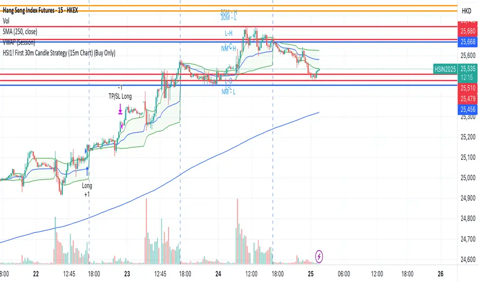
ORB Norman (2 Sessions, Auto Timezone)ORB Norman (2 Sessions, Auto Timezone)
This script plots Opening Range Breakout (ORB) levels for two configurable sessions. It’s designed for intraday traders—especially in futures markets like Gold (GC), Nasdaq (NQ), and S&P (ES)—who trade based on early session breakouts or range rejections. Unlike standard indicators, this tool auto-adjusts for timezones based on the instrument, ensuring precise session alignment.
Features:
Automatically adjusts for NQ/ES (Chicago time) and GC (New York time) based on the symbol.
Plots high, low, and optional midpoint lines for each session.
Clean, minimal settings with visual separation for better usability.
Ray extension length is fully customizable.
Works on any intraday chart (recommended: 5–15 minute timeframes).
Includes customizable session times, colors, ray length, and an optional midpoint line.
Default Sessions:
Session 1:
‣ 07:00–08:00 EST for GC
‣ 06:00–07:00 CT for NQ/ES
Session 2:
‣ 09:30–09:45 EST for GC
‣ 08:30–08:45 CT for NQ/ES
This tool is ideal for traders who scalp the early morning breakout or look for range rejections based on the opening auction.
This script was developed from scratch based on the author's own intraday trading needs.

Tensor Market Analysis Engine (TMAE)# Tensor Market Analysis Engine (TMAE)
## Advanced Multi-Dimensional Mathematical Analysis System
*Where Quantum Mathematics Meets Market Structure*
---
## 🎓 THEORETICAL FOUNDATION
The Tensor Market Analysis Engine represents a revolutionary synthesis of three cutting-edge mathematical frameworks that have never before been combined for comprehensive market analysis. This indicator transcends traditional technical analysis by implementing advanced mathematical concepts from quantum mechanics, information theory, and fractal geometry.
### 🌊 Multi-Dimensional Volatility with Jump Detection
**Hawkes Process Implementation:**
The TMAE employs a sophisticated Hawkes process approximation for detecting self-exciting market jumps. Unlike traditional volatility measures that treat price movements as independent events, the Hawkes process recognizes that market shocks cluster and exhibit memory effects.
**Mathematical Foundation:**
```
Intensity λ(t) = μ + Σ α(t - Tᵢ)
```
Where market jumps at times Tᵢ increase the probability of future jumps through the decay function α, controlled by the Hawkes Decay parameter (0.5-0.99).
**Mahalanobis Distance Calculation:**
The engine calculates volatility jumps using multi-dimensional Mahalanobis distance across up to 5 volatility dimensions:
- **Dimension 1:** Price volatility (standard deviation of returns)
- **Dimension 2:** Volume volatility (normalized volume fluctuations)
- **Dimension 3:** Range volatility (high-low spread variations)
- **Dimension 4:** Correlation volatility (price-volume relationship changes)
- **Dimension 5:** Microstructure volatility (intrabar positioning analysis)
This creates a volatility state vector that captures market behavior impossible to detect with traditional single-dimensional approaches.
### 📐 Hurst Exponent Regime Detection
**Fractal Market Hypothesis Integration:**
The TMAE implements advanced Rescaled Range (R/S) analysis to calculate the Hurst exponent in real-time, providing dynamic regime classification:
- **H > 0.6:** Trending (persistent) markets - momentum strategies optimal
- **H < 0.4:** Mean-reverting (anti-persistent) markets - contrarian strategies optimal
- **H ≈ 0.5:** Random walk markets - breakout strategies preferred
**Adaptive R/S Analysis:**
Unlike static implementations, the TMAE uses adaptive windowing that adjusts to market conditions:
```
H = log(R/S) / log(n)
```
Where R is the range of cumulative deviations and S is the standard deviation over period n.
**Dynamic Regime Classification:**
The system employs hysteresis to prevent regime flipping, requiring sustained Hurst values before regime changes are confirmed. This prevents false signals during transitional periods.
### 🔄 Transfer Entropy Analysis
**Information Flow Quantification:**
Transfer entropy measures the directional flow of information between price and volume, revealing lead-lag relationships that indicate future price movements:
```
TE(X→Y) = Σ p(yₜ₊₁, yₜ, xₜ) log
```
**Causality Detection:**
- **Volume → Price:** Indicates accumulation/distribution phases
- **Price → Volume:** Suggests retail participation or momentum chasing
- **Balanced Flow:** Market equilibrium or transition periods
The system analyzes multiple lag periods (2-20 bars) to capture both immediate and structural information flows.
---
## 🔧 COMPREHENSIVE INPUT SYSTEM
### Core Parameters Group
**Primary Analysis Window (10-100, Default: 50)**
The fundamental lookback period affecting all calculations. Optimization by timeframe:
- **1-5 minute charts:** 20-30 (rapid adaptation to micro-movements)
- **15 minute-1 hour:** 30-50 (balanced responsiveness and stability)
- **4 hour-daily:** 50-100 (smooth signals, reduced noise)
- **Asset-specific:** Cryptocurrency 20-35, Stocks 35-50, Forex 40-60
**Signal Sensitivity (0.1-2.0, Default: 0.7)**
Master control affecting all threshold calculations:
- **Conservative (0.3-0.6):** High-quality signals only, fewer false positives
- **Balanced (0.7-1.0):** Optimal risk-reward ratio for most trading styles
- **Aggressive (1.1-2.0):** Maximum signal frequency, requires careful filtering
**Signal Generation Mode:**
- **Aggressive:** Any component signals (highest frequency)
- **Confluence:** 2+ components agree (balanced approach)
- **Conservative:** All 3 components align (highest quality)
### Volatility Jump Detection Group
**Volatility Dimensions (2-5, Default: 3)**
Determines the mathematical space complexity:
- **2D:** Price + Volume volatility (suitable for clean markets)
- **3D:** + Range volatility (optimal for most conditions)
- **4D:** + Correlation volatility (advanced multi-asset analysis)
- **5D:** + Microstructure volatility (maximum sensitivity)
**Jump Detection Threshold (1.5-4.0σ, Default: 3.0σ)**
Standard deviations required for volatility jump classification:
- **Cryptocurrency:** 2.0-2.5σ (naturally volatile)
- **Stock Indices:** 2.5-3.0σ (moderate volatility)
- **Forex Major Pairs:** 3.0-3.5σ (typically stable)
- **Commodities:** 2.0-3.0σ (varies by commodity)
**Jump Clustering Decay (0.5-0.99, Default: 0.85)**
Hawkes process memory parameter:
- **0.5-0.7:** Fast decay (jumps treated as independent)
- **0.8-0.9:** Moderate clustering (realistic market behavior)
- **0.95-0.99:** Strong clustering (crisis/event-driven markets)
### Hurst Exponent Analysis Group
**Calculation Method Options:**
- **Classic R/S:** Original Rescaled Range (fast, simple)
- **Adaptive R/S:** Dynamic windowing (recommended for trading)
- **DFA:** Detrended Fluctuation Analysis (best for noisy data)
**Trending Threshold (0.55-0.8, Default: 0.60)**
Hurst value defining persistent market behavior:
- **0.55-0.60:** Weak trend persistence
- **0.65-0.70:** Clear trending behavior
- **0.75-0.80:** Strong momentum regimes
**Mean Reversion Threshold (0.2-0.45, Default: 0.40)**
Hurst value defining anti-persistent behavior:
- **0.35-0.45:** Weak mean reversion
- **0.25-0.35:** Clear ranging behavior
- **0.15-0.25:** Strong reversion tendency
### Transfer Entropy Parameters Group
**Information Flow Analysis:**
- **Price-Volume:** Classic flow analysis for accumulation/distribution
- **Price-Volatility:** Risk flow analysis for sentiment shifts
- **Multi-Timeframe:** Cross-timeframe causality detection
**Maximum Lag (2-20, Default: 5)**
Causality detection window:
- **2-5 bars:** Immediate causality (scalping)
- **5-10 bars:** Short-term flow (day trading)
- **10-20 bars:** Structural flow (swing trading)
**Significance Threshold (0.05-0.3, Default: 0.15)**
Minimum entropy for signal generation:
- **0.05-0.10:** Detect subtle information flows
- **0.10-0.20:** Clear causality only
- **0.20-0.30:** Very strong flows only
---
## 🎨 ADVANCED VISUAL SYSTEM
### Tensor Volatility Field Visualization
**Five-Layer Resonance Bands:**
The tensor field creates dynamic support/resistance zones that expand and contract based on mathematical field strength:
- **Core Layer (Purple):** Primary tensor field with highest intensity
- **Layer 2 (Neutral):** Secondary mathematical resonance
- **Layer 3 (Info Blue):** Tertiary harmonic frequencies
- **Layer 4 (Warning Gold):** Outer field boundaries
- **Layer 5 (Success Green):** Maximum field extension
**Field Strength Calculation:**
```
Field Strength = min(3.0, Mahalanobis Distance × Tensor Intensity)
```
The field amplitude adjusts to ATR and mathematical distance, creating dynamic zones that respond to market volatility.
**Radiation Line Network:**
During active tensor states, the system projects directional radiation lines showing field energy distribution:
- **8 Directional Rays:** Complete angular coverage
- **Tapering Segments:** Progressive transparency for natural visual flow
- **Pulse Effects:** Enhanced visualization during volatility jumps
### Dimensional Portal System
**Portal Mathematics:**
Dimensional portals visualize regime transitions using category theory principles:
- **Green Portals (◉):** Trending regime detection (appear below price for support)
- **Red Portals (◎):** Mean-reverting regime (appear above price for resistance)
- **Yellow Portals (○):** Random walk regime (neutral positioning)
**Tensor Trail Effects:**
Each portal generates 8 trailing particles showing mathematical momentum:
- **Large Particles (●):** Strong mathematical signal
- **Medium Particles (◦):** Moderate signal strength
- **Small Particles (·):** Weak signal continuation
- **Micro Particles (˙):** Signal dissipation
### Information Flow Streams
**Particle Stream Visualization:**
Transfer entropy creates flowing particle streams indicating information direction:
- **Upward Streams:** Volume leading price (accumulation phases)
- **Downward Streams:** Price leading volume (distribution phases)
- **Stream Density:** Proportional to information flow strength
**15-Particle Evolution:**
Each stream contains 15 particles with progressive sizing and transparency, creating natural flow visualization that makes information transfer immediately apparent.
### Fractal Matrix Grid System
**Multi-Timeframe Fractal Levels:**
The system calculates and displays fractal highs/lows across five Fibonacci periods:
- **8-Period:** Short-term fractal structure
- **13-Period:** Intermediate-term patterns
- **21-Period:** Primary swing levels
- **34-Period:** Major structural levels
- **55-Period:** Long-term fractal boundaries
**Triple-Layer Visualization:**
Each fractal level uses three-layer rendering:
- **Shadow Layer:** Widest, darkest foundation (width 5)
- **Glow Layer:** Medium white core line (width 3)
- **Tensor Layer:** Dotted mathematical overlay (width 1)
**Intelligent Labeling System:**
Smart spacing prevents label overlap using ATR-based minimum distances. Labels include:
- **Fractal Period:** Time-based identification
- **Topological Class:** Mathematical complexity rating (0, I, II, III)
- **Price Level:** Exact fractal price
- **Mahalanobis Distance:** Current mathematical field strength
- **Hurst Exponent:** Current regime classification
- **Anomaly Indicators:** Visual strength representations (○ ◐ ● ⚡)
### Wick Pressure Analysis
**Rejection Level Mathematics:**
The system analyzes candle wick patterns to project future pressure zones:
- **Upper Wick Analysis:** Identifies selling pressure and resistance zones
- **Lower Wick Analysis:** Identifies buying pressure and support zones
- **Pressure Projection:** Extends lines forward based on mathematical probability
**Multi-Layer Glow Effects:**
Wick pressure lines use progressive transparency (1-8 layers) creating natural glow effects that make pressure zones immediately visible without cluttering the chart.
### Enhanced Regime Background
**Dynamic Intensity Mapping:**
Background colors reflect mathematical regime strength:
- **Deep Transparency (98% alpha):** Subtle regime indication
- **Pulse Intensity:** Based on regime strength calculation
- **Color Coding:** Green (trending), Red (mean-reverting), Neutral (random)
**Smoothing Integration:**
Regime changes incorporate 10-bar smoothing to prevent background flicker while maintaining responsiveness to genuine regime shifts.
### Color Scheme System
**Six Professional Themes:**
- **Dark (Default):** Professional trading environment optimization
- **Light:** High ambient light conditions
- **Classic:** Traditional technical analysis appearance
- **Neon:** High-contrast visibility for active trading
- **Neutral:** Minimal distraction focus
- **Bright:** Maximum visibility for complex setups
Each theme maintains mathematical accuracy while optimizing visual clarity for different trading environments and personal preferences.
---
## 📊 INSTITUTIONAL-GRADE DASHBOARD
### Tensor Field Status Section
**Field Strength Display:**
Real-time Mahalanobis distance calculation with dynamic emoji indicators:
- **⚡ (Lightning):** Extreme field strength (>1.5× threshold)
- **● (Solid Circle):** Strong field activity (>1.0× threshold)
- **○ (Open Circle):** Normal field state
**Signal Quality Rating:**
Democratic algorithm assessment:
- **ELITE:** All 3 components aligned (highest probability)
- **STRONG:** 2 components aligned (good probability)
- **GOOD:** 1 component active (moderate probability)
- **WEAK:** No clear component signals
**Threshold and Anomaly Monitoring:**
- **Threshold Display:** Current mathematical threshold setting
- **Anomaly Level (0-100%):** Combined volatility and volume spike measurement
- **>70%:** High anomaly (red warning)
- **30-70%:** Moderate anomaly (orange caution)
- **<30%:** Normal conditions (green confirmation)
### Tensor State Analysis Section
**Mathematical State Classification:**
- **↑ BULL (Tensor State +1):** Trending regime with bullish bias
- **↓ BEAR (Tensor State -1):** Mean-reverting regime with bearish bias
- **◈ SUPER (Tensor State 0):** Random walk regime (neutral)
**Visual State Gauge:**
Five-circle progression showing tensor field polarity:
- **🟢🟢🟢⚪⚪:** Strong bullish mathematical alignment
- **⚪⚪🟡⚪⚪:** Neutral/transitional state
- **⚪⚪🔴🔴🔴:** Strong bearish mathematical alignment
**Trend Direction and Phase Analysis:**
- **📈 BULL / 📉 BEAR / ➡️ NEUTRAL:** Primary trend classification
- **🌪️ CHAOS:** Extreme information flow (>2.0 flow strength)
- **⚡ ACTIVE:** Strong information flow (1.0-2.0 flow strength)
- **😴 CALM:** Low information flow (<1.0 flow strength)
### Trading Signals Section
**Real-Time Signal Status:**
- **🟢 ACTIVE / ⚪ INACTIVE:** Long signal availability
- **🔴 ACTIVE / ⚪ INACTIVE:** Short signal availability
- **Components (X/3):** Active algorithmic components
- **Mode Display:** Current signal generation mode
**Signal Strength Visualization:**
Color-coded component count:
- **Green:** 3/3 components (maximum confidence)
- **Aqua:** 2/3 components (good confidence)
- **Orange:** 1/3 components (moderate confidence)
- **Gray:** 0/3 components (no signals)
### Performance Metrics Section
**Win Rate Monitoring:**
Estimated win rates based on signal quality with emoji indicators:
- **🔥 (Fire):** ≥60% estimated win rate
- **👍 (Thumbs Up):** 45-59% estimated win rate
- **⚠️ (Warning):** <45% estimated win rate
**Mathematical Metrics:**
- **Hurst Exponent:** Real-time fractal dimension (0.000-1.000)
- **Information Flow:** Volume/price leading indicators
- **📊 VOL:** Volume leading price (accumulation/distribution)
- **💰 PRICE:** Price leading volume (momentum/speculation)
- **➖ NONE:** Balanced information flow
- **Volatility Classification:**
- **🔥 HIGH:** Above 1.5× jump threshold
- **📊 NORM:** Normal volatility range
- **😴 LOW:** Below 0.5× jump threshold
### Market Structure Section (Large Dashboard)
**Regime Classification:**
- **📈 TREND:** Hurst >0.6, momentum strategies optimal
- **🔄 REVERT:** Hurst <0.4, contrarian strategies optimal
- **🎲 RANDOM:** Hurst ≈0.5, breakout strategies preferred
**Mathematical Field Analysis:**
- **Dimensions:** Current volatility space complexity (2D-5D)
- **Hawkes λ (Lambda):** Self-exciting jump intensity (0.00-1.00)
- **Jump Status:** 🚨 JUMP (active) / ✅ NORM (normal)
### Settings Summary Section (Large Dashboard)
**Active Configuration Display:**
- **Sensitivity:** Current master sensitivity setting
- **Lookback:** Primary analysis window
- **Theme:** Active color scheme
- **Method:** Hurst calculation method (Classic R/S, Adaptive R/S, DFA)
**Dashboard Sizing Options:**
- **Small:** Essential metrics only (mobile/small screens)
- **Normal:** Balanced information density (standard desktop)
- **Large:** Maximum detail (multi-monitor setups)
**Position Options:**
- **Top Right:** Standard placement (avoids price action)
- **Top Left:** Wide chart optimization
- **Bottom Right:** Recent price focus (scalping)
- **Bottom Left:** Maximum price visibility (swing trading)
---
## 🎯 SIGNAL GENERATION LOGIC
### Multi-Component Convergence System
**Component Signal Architecture:**
The TMAE generates signals through sophisticated component analysis rather than simple threshold crossing:
**Volatility Component:**
- **Jump Detection:** Mahalanobis distance threshold breach
- **Hawkes Intensity:** Self-exciting process activation (>0.2)
- **Multi-dimensional:** Considers all volatility dimensions simultaneously
**Hurst Regime Component:**
- **Trending Markets:** Price above SMA-20 with positive momentum
- **Mean-Reverting Markets:** Price at Bollinger Band extremes
- **Random Markets:** Bollinger squeeze breakouts with directional confirmation
**Transfer Entropy Component:**
- **Volume Leadership:** Information flow from volume to price
- **Volume Spike:** Volume 110%+ above 20-period average
- **Flow Significance:** Above entropy threshold with directional bias
### Democratic Signal Weighting
**Signal Mode Implementation:**
- **Aggressive Mode:** Any single component triggers signal
- **Confluence Mode:** Minimum 2 components must agree
- **Conservative Mode:** All 3 components must align
**Momentum Confirmation:**
All signals require momentum confirmation:
- **Long Signals:** RSI >50 AND price >EMA-9
- **Short Signals:** RSI <50 AND price 0.6):**
- **Increase Sensitivity:** Catch momentum continuation
- **Lower Mean Reversion Threshold:** Avoid counter-trend signals
- **Emphasize Volume Leadership:** Institutional accumulation/distribution
- **Tensor Field Focus:** Use expansion for trend continuation
- **Signal Mode:** Aggressive or Confluence for trend following
**Range-Bound Markets (Hurst <0.4):**
- **Decrease Sensitivity:** Avoid false breakouts
- **Lower Trending Threshold:** Quick regime recognition
- **Focus on Price Leadership:** Retail sentiment extremes
- **Fractal Grid Emphasis:** Support/resistance trading
- **Signal Mode:** Conservative for high-probability reversals
**Volatile Markets (High Jump Frequency):**
- **Increase Hawkes Decay:** Recognize event clustering
- **Higher Jump Threshold:** Avoid noise signals
- **Maximum Dimensions:** Capture full volatility complexity
- **Reduce Position Sizing:** Risk management adaptation
- **Enhanced Visuals:** Maximum information for rapid decisions
**Low Volatility Markets (Low Jump Frequency):**
- **Decrease Jump Threshold:** Capture subtle movements
- **Lower Hawkes Decay:** Treat moves as independent
- **Reduce Dimensions:** Simplify analysis
- **Increase Position Sizing:** Capitalize on compressed volatility
- **Minimal Visuals:** Reduce distraction in quiet markets
---
## 🚀 ADVANCED TRADING STRATEGIES
### The Mathematical Convergence Method
**Entry Protocol:**
1. **Fractal Grid Approach:** Monitor price approaching significant fractal levels
2. **Tensor Field Confirmation:** Verify field expansion supporting direction
3. **Portal Signal:** Wait for dimensional portal appearance
4. **ELITE/STRONG Quality:** Only trade highest quality mathematical signals
5. **Component Consensus:** Confirm 2+ components agree in Confluence mode
**Example Implementation:**
- Price approaching 21-period fractal high
- Tensor field expanding upward (bullish mathematical alignment)
- Green portal appears below price (trending regime confirmation)
- ELITE quality signal with 3/3 components active
- Enter long position with stop below fractal level
**Risk Management:**
- **Stop Placement:** Below/above fractal level that generated signal
- **Position Sizing:** Based on Mahalanobis distance (higher distance = smaller size)
- **Profit Targets:** Next fractal level or tensor field resistance
### The Regime Transition Strategy
**Regime Change Detection:**
1. **Monitor Hurst Exponent:** Watch for persistent moves above/below thresholds
2. **Portal Color Change:** Regime transitions show different portal colors
3. **Background Intensity:** Increasing regime background intensity
4. **Mathematical Confirmation:** Wait for regime confirmation (hysteresis)
**Trading Implementation:**
- **Trending Transitions:** Trade momentum breakouts, follow trend
- **Mean Reversion Transitions:** Trade range boundaries, fade extremes
- **Random Transitions:** Trade breakouts with tight stops
**Advanced Techniques:**
- **Multi-Timeframe:** Confirm regime on higher timeframe
- **Early Entry:** Enter on regime transition rather than confirmation
- **Regime Strength:** Larger positions during strong regime signals
### The Information Flow Momentum Strategy
**Flow Detection Protocol:**
1. **Monitor Transfer Entropy:** Watch for significant information flow shifts
2. **Volume Leadership:** Strong edge when volume leads price
3. **Flow Acceleration:** Increasing flow strength indicates momentum
4. **Directional Confirmation:** Ensure flow aligns with intended trade direction
**Entry Signals:**
- **Volume → Price Flow:** Enter during accumulation/distribution phases
- **Price → Volume Flow:** Enter on momentum confirmation breaks
- **Flow Reversal:** Counter-trend entries when flow reverses
**Optimization:**
- **Scalping:** Use immediate flow detection (2-5 bar lag)
- **Swing Trading:** Use structural flow (10-20 bar lag)
- **Multi-Asset:** Compare flow between correlated assets
### The Tensor Field Expansion Strategy
**Field Mathematics:**
The tensor field expansion indicates mathematical pressure building in market structure:
**Expansion Phases:**
1. **Compression:** Field contracts, volatility decreases
2. **Tension Building:** Mathematical pressure accumulates
3. **Expansion:** Field expands rapidly with directional movement
4. **Resolution:** Field stabilizes at new equilibrium
**Trading Applications:**
- **Compression Trading:** Prepare for breakout during field contraction
- **Expansion Following:** Trade direction of field expansion
- **Reversion Trading:** Fade extreme field expansion
- **Multi-Dimensional:** Consider all field layers for confirmation
### The Hawkes Process Event Strategy
**Self-Exciting Jump Trading:**
Understanding that market shocks cluster and create follow-on opportunities:
**Jump Sequence Analysis:**
1. **Initial Jump:** First volatility jump detected
2. **Clustering Phase:** Hawkes intensity remains elevated
3. **Follow-On Opportunities:** Additional jumps more likely
4. **Decay Period:** Intensity gradually decreases
**Implementation:**
- **Jump Confirmation:** Wait for mathematical jump confirmation
- **Direction Assessment:** Use other components for direction
- **Clustering Trades:** Trade subsequent moves during high intensity
- **Decay Exit:** Exit positions as Hawkes intensity decays
### The Fractal Confluence System
**Multi-Timeframe Fractal Analysis:**
Combining fractal levels across different periods for high-probability zones:
**Confluence Zones:**
- **Double Confluence:** 2 fractal levels align
- **Triple Confluence:** 3+ fractal levels cluster
- **Mathematical Confirmation:** Tensor field supports the level
- **Information Flow:** Transfer entropy confirms direction
**Trading Protocol:**
1. **Identify Confluence:** Find 2+ fractal levels within 1 ATR
2. **Mathematical Support:** Verify tensor field alignment
3. **Signal Quality:** Wait for STRONG or ELITE signal
4. **Risk Definition:** Use fractal level for stop placement
5. **Profit Targeting:** Next major fractal confluence zone
---
## ⚠️ COMPREHENSIVE RISK MANAGEMENT
### Mathematical Position Sizing
**Mahalanobis Distance Integration:**
Position size should inversely correlate with mathematical field strength:
```
Position Size = Base Size × (Threshold / Mahalanobis Distance)
```
**Risk Scaling Matrix:**
- **Low Field Strength (<2.0):** Standard position sizing
- **Moderate Field Strength (2.0-3.0):** 75% position sizing
- **High Field Strength (3.0-4.0):** 50% position sizing
- **Extreme Field Strength (>4.0):** 25% position sizing or no trade
### Signal Quality Risk Adjustment
**Quality-Based Position Sizing:**
- **ELITE Signals:** 100% of planned position size
- **STRONG Signals:** 75% of planned position size
- **GOOD Signals:** 50% of planned position size
- **WEAK Signals:** No position or paper trading only
**Component Agreement Scaling:**
- **3/3 Components:** Full position size
- **2/3 Components:** 75% position size
- **1/3 Components:** 50% position size or skip trade
### Regime-Adaptive Risk Management
**Trending Market Risk:**
- **Wider Stops:** Allow for trend continuation
- **Trend Following:** Trade with regime direction
- **Higher Position Size:** Trend probability advantage
- **Momentum Stops:** Trail stops based on momentum indicators
**Mean-Reverting Market Risk:**
- **Tighter Stops:** Quick exits on trend continuation
- **Contrarian Positioning:** Trade against extremes
- **Smaller Position Size:** Higher reversal failure rate
- **Level-Based Stops:** Use fractal levels for stops
**Random Market Risk:**
- **Breakout Focus:** Trade only clear breakouts
- **Tight Initial Stops:** Quick exit if breakout fails
- **Reduced Frequency:** Skip marginal setups
- **Range-Based Targets:** Profit targets at range boundaries
### Volatility-Adaptive Risk Controls
**High Volatility Periods:**
- **Reduced Position Size:** Account for wider price swings
- **Wider Stops:** Avoid noise-based exits
- **Lower Frequency:** Skip marginal setups
- **Faster Exits:** Take profits more quickly
**Low Volatility Periods:**
- **Standard Position Size:** Normal risk parameters
- **Tighter Stops:** Take advantage of compressed ranges
- **Higher Frequency:** Trade more setups
- **Extended Targets:** Allow for compressed volatility expansion
### Multi-Timeframe Risk Alignment
**Higher Timeframe Trend:**
- **With Trend:** Standard or increased position size
- **Against Trend:** Reduced position size or skip
- **Neutral Trend:** Standard position size with tight management
**Risk Hierarchy:**
1. **Primary:** Current timeframe signal quality
2. **Secondary:** Higher timeframe trend alignment
3. **Tertiary:** Mathematical field strength
4. **Quaternary:** Market regime classification
---
## 📚 EDUCATIONAL VALUE AND MATHEMATICAL CONCEPTS
### Advanced Mathematical Concepts
**Tensor Analysis in Markets:**
The TMAE introduces traders to tensor analysis, a branch of mathematics typically reserved for physics and advanced engineering. Tensors provide a framework for understanding multi-dimensional market relationships that scalar and vector analysis cannot capture.
**Information Theory Applications:**
Transfer entropy implementation teaches traders about information flow in markets, a concept from information theory that quantifies directional causality between variables. This provides intuition about market microstructure and participant behavior.
**Fractal Geometry in Trading:**
The Hurst exponent calculation exposes traders to fractal geometry concepts, helping understand that markets exhibit self-similar patterns across multiple timeframes. This mathematical insight transforms how traders view market structure.
**Stochastic Process Theory:**
The Hawkes process implementation introduces concepts from stochastic process theory, specifically self-exciting point processes. This provides mathematical framework for understanding why market events cluster and exhibit memory effects.
### Learning Progressive Complexity
**Beginner Mathematical Concepts:**
- **Volatility Dimensions:** Understanding multi-dimensional analysis
- **Regime Classification:** Learning market personality types
- **Signal Democracy:** Algorithmic consensus building
- **Visual Mathematics:** Interpreting mathematical concepts visually
**Intermediate Mathematical Applications:**
- **Mahalanobis Distance:** Statistical distance in multi-dimensional space
- **Rescaled Range Analysis:** Fractal dimension measurement
- **Information Entropy:** Quantifying uncertainty and causality
- **Field Theory:** Understanding mathematical fields in market context
**Advanced Mathematical Integration:**
- **Tensor Field Dynamics:** Multi-dimensional market force analysis
- **Stochastic Self-Excitation:** Event clustering and memory effects
- **Categorical Composition:** Mathematical signal combination theory
- **Topological Market Analysis:** Understanding market shape and connectivity
### Practical Mathematical Intuition
**Developing Market Mathematics Intuition:**
The TMAE serves as a bridge between abstract mathematical concepts and practical trading applications. Traders develop intuitive understanding of:
- **How markets exhibit mathematical structure beneath apparent randomness**
- **Why multi-dimensional analysis reveals patterns invisible to single-variable approaches**
- **How information flows through markets in measurable, predictable ways**
- **Why mathematical models provide probabilistic edges rather than certainties**
---
## 🔬 IMPLEMENTATION AND OPTIMIZATION
### Getting Started Protocol
**Phase 1: Observation (Week 1)**
1. **Apply with defaults:** Use standard settings on your primary trading timeframe
2. **Study visual elements:** Learn to interpret tensor fields, portals, and streams
3. **Monitor dashboard:** Observe how metrics change with market conditions
4. **No trading:** Focus entirely on pattern recognition and understanding
**Phase 2: Pattern Recognition (Week 2-3)**
1. **Identify signal patterns:** Note what market conditions produce different signal qualities
2. **Regime correlation:** Observe how Hurst regimes affect signal performance
3. **Visual confirmation:** Learn to read tensor field expansion and portal signals
4. **Component analysis:** Understand which components drive signals in different markets
**Phase 3: Parameter Optimization (Week 4-5)**
1. **Asset-specific tuning:** Adjust parameters for your specific trading instrument
2. **Timeframe optimization:** Fine-tune for your preferred trading timeframe
3. **Sensitivity adjustment:** Balance signal frequency with quality
4. **Visual customization:** Optimize colors and intensity for your trading environment
**Phase 4: Live Implementation (Week 6+)**
1. **Paper trading:** Test signals with hypothetical trades
2. **Small position sizing:** Begin with minimal risk during learning phase
3. **Performance tracking:** Monitor actual vs. expected signal performance
4. **Continuous optimization:** Refine settings based on real performance data
### Performance Monitoring System
**Signal Quality Tracking:**
- **ELITE Signal Win Rate:** Track highest quality signals separately
- **Component Performance:** Monitor which components provide best signals
- **Regime Performance:** Analyze performance across different market regimes
- **Timeframe Analysis:** Compare performance across different session times
**Mathematical Metric Correlation:**
- **Field Strength vs. Performance:** Higher field strength should correlate with better performance
- **Component Agreement vs. Win Rate:** More component agreement should improve win rates
- **Regime Alignment vs. Success:** Trading with mathematical regime should outperform
### Continuous Optimization Process
**Monthly Review Protocol:**
1. **Performance Analysis:** Review win rates, profit factors, and maximum drawdown
2. **Parameter Assessment:** Evaluate if current settings remain optimal
3. **Market Adaptation:** Adjust for changes in market character or volatility
4. **Component Weighting:** Consider if certain components should receive more/less emphasis
**Quarterly Deep Analysis:**
1. **Mathematical Model Validation:** Verify that mathematical relationships remain valid
2. **Regime Distribution:** Analyze time spent in different market regimes
3. **Signal Evolution:** Track how signal characteristics change over time
4. **Correlation Analysis:** Monitor correlations between different mathematical components
---
## 🌟 UNIQUE INNOVATIONS AND CONTRIBUTIONS
### Revolutionary Mathematical Integration
**First-Ever Implementations:**
1. **Multi-Dimensional Volatility Tensor:** First indicator to implement true tensor analysis for market volatility
2. **Real-Time Hawkes Process:** First trading implementation of self-exciting point processes
3. **Transfer Entropy Trading Signals:** First practical application of information theory for trade generation
4. **Democratic Component Voting:** First algorithmic consensus system for signal generation
5. **Fractal-Projected Signal Quality:** First system to predict signal quality at future price levels
### Advanced Visualization Innovations
**Mathematical Visualization Breakthroughs:**
- **Tensor Field Radiation:** Visual representation of mathematical field energy
- **Dimensional Portal System:** Category theory visualization for regime transitions
- **Information Flow Streams:** Real-time visual display of market information transfer
- **Multi-Layer Fractal Grid:** Intelligent spacing and projection system
- **Regime Intensity Mapping:** Dynamic background showing mathematical regime strength
### Practical Trading Innovations
**Trading System Advances:**
- **Quality-Weighted Signal Generation:** Signals rated by mathematical confidence
- **Regime-Adaptive Strategy Selection:** Automatic strategy optimization based on market personality
- **Anti-Spam Signal Protection:** Mathematical prevention of signal clustering
- **Component Performance Tracking:** Real-time monitoring of algorithmic component success
- **Field-Strength Position Sizing:** Mathematical volatility integration for risk management
---
## ⚖️ RESPONSIBLE USAGE AND LIMITATIONS
### Mathematical Model Limitations
**Understanding Model Boundaries:**
While the TMAE implements sophisticated mathematical concepts, traders must understand fundamental limitations:
- **Markets Are Not Purely Mathematical:** Human psychology, news events, and fundamental factors create unpredictable elements
- **Past Performance Limitations:** Mathematical relationships that worked historically may not persist indefinitely
- **Model Risk:** Complex models can fail during unprecedented market conditions
- **Overfitting Potential:** Highly optimized parameters may not generalize to future market conditions
### Proper Implementation Guidelines
**Risk Management Requirements:**
- **Never Risk More Than 2% Per Trade:** Regardless of signal quality
- **Diversification Mandatory:** Don't rely solely on mathematical signals
- **Position Sizing Discipline:** Use mathematical field strength for sizing, not confidence
- **Stop Loss Non-Negotiable:** Every trade must have predefined risk parameters
**Realistic Expectations:**
- **Mathematical Edge, Not Certainty:** The indicator provides probabilistic advantages, not guaranteed outcomes
- **Learning Curve Required:** Complex mathematical concepts require time to master
- **Market Adaptation Necessary:** Parameters must evolve with changing market conditions
- **Continuous Education Important:** Understanding underlying mathematics improves application
### Ethical Trading Considerations
**Market Impact Awareness:**
- **Information Asymmetry:** Advanced mathematical analysis may provide advantages over other market participants
- **Position Size Responsibility:** Large positions based on mathematical signals can impact market structure
- **Sharing Knowledge:** Consider educational contributions to trading community
- **Fair Market Participation:** Use mathematical advantages responsibly within market framework
### Professional Development Path
**Skill Development Sequence:**
1. **Basic Mathematical Literacy:** Understand fundamental concepts before advanced application
2. **Risk Management Mastery:** Develop disciplined risk control before relying on complex signals
3. **Market Psychology Understanding:** Combine mathematical analysis with behavioral market insights
4. **Continuous Learning:** Stay updated on mathematical finance developments and market evolution
---
## 🔮 CONCLUSION
The Tensor Market Analysis Engine represents a quantum leap forward in technical analysis, successfully bridging the gap between advanced pure mathematics and practical trading applications. By integrating multi-dimensional volatility analysis, fractal market theory, and information flow dynamics, the TMAE reveals market structure invisible to conventional analysis while maintaining visual clarity and practical usability.
### Mathematical Innovation Legacy
This indicator establishes new paradigms in technical analysis:
- **Tensor analysis for market volatility understanding**
- **Stochastic self-excitation for event clustering prediction**
- **Information theory for causality-based trade generation**
- **Democratic algorithmic consensus for signal quality enhancement**
- **Mathematical field visualization for intuitive market understanding**
### Practical Trading Revolution
Beyond mathematical innovation, the TMAE transforms practical trading:
- **Quality-rated signals replace binary buy/sell decisions**
- **Regime-adaptive strategies automatically optimize for market personality**
- **Multi-dimensional risk management integrates mathematical volatility measures**
- **Visual mathematical concepts make complex analysis immediately interpretable**
- **Educational value creates lasting improvement in trading understanding**
### Future-Proof Design
The mathematical foundations ensure lasting relevance:
- **Universal mathematical principles transcend market evolution**
- **Multi-dimensional analysis adapts to new market structures**
- **Regime detection automatically adjusts to changing market personalities**
- **Component democracy allows for future algorithmic additions**
- **Mathematical visualization scales with increasing market complexity**
### Commitment to Excellence
The TMAE represents more than an indicator—it embodies a philosophy of bringing rigorous mathematical analysis to trading while maintaining practical utility and visual elegance. Every component, from the multi-dimensional tensor fields to the democratic signal generation, reflects a commitment to mathematical accuracy, trading practicality, and educational value.
### Trading with Mathematical Precision
In an era where markets grow increasingly complex and computational, the TMAE provides traders with mathematical tools previously available only to institutional quantitative research teams. Yet unlike academic mathematical models, the TMAE translates complex concepts into intuitive visual representations and practical trading signals.
By combining the mathematical rigor of tensor analysis, the statistical power of multi-dimensional volatility modeling, and the information-theoretic insights of transfer entropy, traders gain unprecedented insight into market structure and dynamics.
### Final Perspective
Markets, like nature, exhibit profound mathematical beauty beneath apparent chaos. The Tensor Market Analysis Engine serves as a mathematical lens that reveals this hidden order, transforming how traders perceive and interact with market structure.
Through mathematical precision, visual elegance, and practical utility, the TMAE empowers traders to see beyond the noise and trade with the confidence that comes from understanding the mathematical principles governing market behavior.
Trade with mathematical insight. Trade with the power of tensors. Trade with the TMAE.
*"In mathematics, you don't understand things. You just get used to them." - John von Neumann*
*With the TMAE, mathematical market understanding becomes not just possible, but intuitive.*
— Dskyz, Trade with insight. Trade with anticipation.

Langlands-Operadic Möbius Vortex (LOMV)Langlands-Operadic Möbius Vortex (LOMV)
Where Pure Mathematics Meets Market Reality
A Revolutionary Synthesis of Number Theory, Category Theory, and Market Dynamics
🎓 THEORETICAL FOUNDATION
The Langlands-Operadic Möbius Vortex represents a groundbreaking fusion of three profound mathematical frameworks that have never before been combined for market analysis:
The Langlands Program: Harmonic Analysis in Markets
Developed by Robert Langlands (Fields Medal recipient), the Langlands Program creates bridges between number theory, algebraic geometry, and harmonic analysis. In our indicator:
L-Function Implementation:
- Utilizes the Möbius function μ(n) for weighted price analysis
- Applies Riemann zeta function convergence principles
- Calculates quantum harmonic resonance between -2 and +2
- Measures deep mathematical patterns invisible to traditional analysis
The L-Function core calculation employs:
L_sum = Σ(return_val × μ(n) × n^(-s))
Where s is the critical strip parameter (0.5-2.5), controlling mathematical precision and signal smoothness.
Operadic Composition Theory: Multi-Strategy Democracy
Category theory and operads provide the mathematical framework for composing multiple trading strategies into a unified signal. This isn't simple averaging - it's mathematical composition using:
Strategy Composition Arity (2-5 strategies):
- Momentum analysis via RSI transformation
- Mean reversion through Bollinger Band mathematics
- Order Flow Polarity Index (revolutionary T3-smoothed volume analysis)
- Trend detection using Directional Movement
- Higher timeframe momentum confirmation
Agreement Threshold System: Democratic voting where strategies must reach consensus before signal generation. This prevents false signals during market uncertainty.
Möbius Function: Number Theory in Action
The Möbius function μ(n) forms the mathematical backbone:
- μ(n) = 1 if n is a square-free positive integer with even number of prime factors
- μ(n) = -1 if n is a square-free positive integer with odd number of prime factors
- μ(n) = 0 if n has a squared prime factor
This creates oscillating weights that reveal hidden market periodicities and harmonic structures.
🔧 COMPREHENSIVE INPUT SYSTEM
Langlands Program Parameters
Modular Level N (5-50, default 30):
Primary lookback for quantum harmonic analysis. Optimized by timeframe:
- Scalping (1-5min): 15-25
- Day Trading (15min-1H): 25-35
- Swing Trading (4H-1D): 35-50
- Asset-specific: Crypto 15-25, Stocks 30-40, Forex 35-45
L-Function Critical Strip (0.5-2.5, default 1.5):
Controls Riemann zeta convergence precision:
- Higher values: More stable, smoother signals
- Lower values: More reactive, catches quick moves
- High frequency: 0.8-1.2, Medium: 1.3-1.7, Low: 1.8-2.3
Frobenius Trace Period (5-50, default 21):
Galois representation lookback for price-volume correlation:
- Measures harmonic relationships in market flows
- Scalping: 8-15, Day Trading: 18-25, Swing: 25-40
HTF Multi-Scale Analysis:
Higher timeframe context prevents trading against major trends:
- Provides market bias and filters signals
- Improves win rates by 15-25% through trend alignment
Operadic Composition Parameters
Strategy Composition Arity (2-5, default 4):
Number of algorithms composed for final signal:
- Conservative: 4-5 strategies (higher confidence)
- Moderate: 3-4 strategies (balanced approach)
- Aggressive: 2-3 strategies (more frequent signals)
Category Agreement Threshold (2-5, default 3):
Democratic voting minimum for signal generation:
- Higher agreement: Fewer but higher quality signals
- Lower agreement: More signals, potential false positives
Swiss-Cheese Mixing (0.1-0.5, default 0.382):
Golden ratio φ⁻¹ based blending of trend factors:
- 0.382 is φ⁻¹, optimal for natural market fractals
- Higher values: Stronger trend following
- Lower values: More contrarian signals
OFPI Configuration:
- OFPI Length (5-30, default 14): Order Flow calculation period
- T3 Smoothing (3-10, default 5): Advanced exponential smoothing
- T3 Volume Factor (0.5-1.0, default 0.7): Smoothing aggressiveness control
Unified Scoring System
Component Weights (sum ≈ 1.0):
- L-Function Weight (0.1-0.5, default 0.3): Mathematical harmony emphasis
- Galois Rank Weight (0.1-0.5, default 0.2): Market structure complexity
- Operadic Weight (0.1-0.5, default 0.3): Multi-strategy consensus
- Correspondence Weight (0.1-0.5, default 0.2): Theory-practice alignment
Signal Threshold (0.5-10.0, default 5.0):
Quality filter producing:
- 8.0+: EXCEPTIONAL signals only
- 6.0-7.9: STRONG signals
- 4.0-5.9: MODERATE signals
- 2.0-3.9: WEAK signals
🎨 ADVANCED VISUAL SYSTEM
Multi-Dimensional Quantum Aura Bands
Five-layer resonance field showing market energy:
- Colors: Theme-matched gradients (Quantum purple, Holographic cyan, etc.)
- Expansion: Dynamic based on score intensity and volatility
- Function: Multi-timeframe support/resistance zones
Morphism Flow Portals
Category theory visualization showing market topology:
- Green/Cyan Portals: Bullish mathematical flow
- Red/Orange Portals: Bearish mathematical flow
- Size/Intensity: Proportional to signal strength
- Recursion Depth (1-8): Nested patterns for flow evolution
Fractal Grid System
Dynamic support/resistance with projected L-Scores:
- Multiple Timeframes: 10, 20, 30, 40, 50-period highs/lows
- Smart Spacing: Prevents level overlap using ATR-based minimum distance
- Projections: Estimated signal scores when price reaches levels
- Usage: Precise entry/exit timing with mathematical confirmation
Wick Pressure Analysis
Rejection level prediction using candle mathematics:
- Upper Wicks: Selling pressure zones (purple/red lines)
- Lower Wicks: Buying pressure zones (purple/green lines)
- Glow Intensity (1-8): Visual emphasis and line reach
- Application: Confluence with fractal grid creates high-probability zones
Regime Intensity Heatmap
Background coloring showing market energy:
- Black/Dark: Low activity, range-bound markets
- Purple Glow: Building momentum and trend development
- Bright Purple: High activity, strong directional moves
- Calculation: Combines trend, momentum, volatility, and score intensity
Six Professional Themes
- Quantum: Purple/violet for general trading and mathematical focus
- Holographic: Cyan/magenta optimized for cryptocurrency markets
- Crystalline: Blue/turquoise for conservative, stability-focused trading
- Plasma: Gold/magenta for high-energy volatility trading
- Cosmic Neon: Bright neon colors for maximum visibility and aggressive trading
📊 INSTITUTIONAL-GRADE DASHBOARD
Unified AI Score Section
- Total Score (-10 to +10): Primary decision metric
- >5: Strong bullish signals
- <-5: Strong bearish signals
- Quality ratings: EXCEPTIONAL > STRONG > MODERATE > WEAK
- Component Analysis: Individual L-Function, Galois, Operadic, and Correspondence contributions
Order Flow Analysis
Revolutionary OFPI integration:
- OFPI Value (-100% to +100%): Real buying vs selling pressure
- Visual Gauge: Horizontal bar chart showing flow intensity
- Momentum Status: SHIFTING, ACCELERATING, STRONG, MODERATE, or WEAK
- Trading Application: Flow shifts often precede major moves
Signal Performance Tracking
- Win Rate Monitoring: Real-time success percentage with emoji indicators
- Signal Count: Total signals generated for frequency analysis
- Current Position: LONG, SHORT, or NONE with P&L tracking
- Volatility Regime: HIGH, MEDIUM, or LOW classification
Market Structure Analysis
- Möbius Field Strength: Mathematical field oscillation intensity
- CHAOTIC: High complexity, use wider stops
- STRONG: Active field, normal position sizing
- MODERATE: Balanced conditions
- WEAK: Low activity, consider smaller positions
- HTF Trend: Higher timeframe bias (BULL/BEAR/NEUTRAL)
- Strategy Agreement: Multi-algorithm consensus level
Position Management
When in trades, displays:
- Entry Price: Original signal price
- Current P&L: Real-time percentage with risk level assessment
- Duration: Bars in trade for timing analysis
- Risk Level: HIGH/MEDIUM/LOW based on current exposure
🚀 SIGNAL GENERATION LOGIC
Balanced Long/Short Architecture
The indicator generates signals through multiple convergent pathways:
Long Entry Conditions:
- Score threshold breach with algorithmic agreement
- Strong bullish order flow (OFPI > 0.15) with positive composite signal
- Bullish pattern recognition with mathematical confirmation
- HTF trend alignment with momentum shifting
- Extreme bullish OFPI (>0.3) with any positive score
Short Entry Conditions:
- Score threshold breach with bearish agreement
- Strong bearish order flow (OFPI < -0.15) with negative composite signal
- Bearish pattern recognition with mathematical confirmation
- HTF trend alignment with momentum shifting
- Extreme bearish OFPI (<-0.3) with any negative score
Exit Logic:
- Score deterioration below continuation threshold
- Signal quality degradation
- Opposing order flow acceleration
- 10-bar minimum between signals prevents overtrading
⚙️ OPTIMIZATION GUIDELINES
Asset-Specific Settings
Cryptocurrency Trading:
- Modular Level: 15-25 (capture volatility)
- L-Function Precision: 0.8-1.3 (reactive to price swings)
- OFPI Length: 10-20 (fast correlation shifts)
- Cascade Levels: 5-7, Theme: Holographic
Stock Index Trading:
- Modular Level: 25-35 (balanced trending)
- L-Function Precision: 1.5-1.8 (stable patterns)
- OFPI Length: 14-20 (standard correlation)
- Cascade Levels: 4-5, Theme: Quantum
Forex Trading:
- Modular Level: 35-45 (smooth trends)
- L-Function Precision: 1.6-2.1 (high smoothing)
- OFPI Length: 18-25 (disable volume amplification)
- Cascade Levels: 3-4, Theme: Crystalline
Timeframe Optimization
Scalping (1-5 minute charts):
- Reduce all lookback parameters by 30-40%
- Increase L-Function precision for noise reduction
- Enable all visual elements for maximum information
- Use Small dashboard to save screen space
Day Trading (15 minute - 1 hour):
- Use default parameters as starting point
- Adjust based on market volatility
- Normal dashboard provides optimal information density
- Focus on OFPI momentum shifts for entries
Swing Trading (4 hour - Daily):
- Increase lookback parameters by 30-50%
- Higher L-Function precision for stability
- Large dashboard for comprehensive analysis
- Emphasize HTF trend alignment
🏆 ADVANCED TRADING STRATEGIES
The Mathematical Confluence Method
1. Wait for Fractal Grid level approach
2. Confirm with projected L-Score > threshold
3. Verify OFPI alignment with direction
4. Enter on portal signal with quality ≥ STRONG
5. Exit on score deterioration or opposing flow
The Regime Trading System
1. Monitor Aether Flow background intensity
2. Trade aggressively during bright purple periods
3. Reduce position size during dark periods
4. Use Möbius Field strength for stop placement
5. Align with HTF trend for maximum probability
The OFPI Momentum Strategy
1. Watch for momentum shifting detection
2. Confirm with accelerating flow in direction
3. Enter on immediate portal signal
4. Scale out at Fibonacci levels
5. Exit on flow deceleration or reversal
⚠️ RISK MANAGEMENT INTEGRATION
Mathematical Position Sizing
- Use Galois Rank for volatility-adjusted sizing
- Möbius Field strength determines stop width
- Fractal Dimension guides maximum exposure
- OFPI momentum affects entry timing
Signal Quality Filtering
- Trade only STRONG or EXCEPTIONAL quality signals
- Increase position size with higher agreement levels
- Reduce risk during CHAOTIC Möbius field periods
- Respect HTF trend alignment for directional bias
🔬 DEVELOPMENT JOURNEY
Creating the LOMV was an extraordinary mathematical undertaking that pushed the boundaries of what's possible in technical analysis. This indicator almost didn't happen. The theoretical complexity nearly proved insurmountable.
The Mathematical Challenge
Implementing the Langlands Program required deep research into:
- Number theory and the Möbius function
- Riemann zeta function convergence properties
- L-function analytical continuation
- Galois representations in finite fields
The mathematical literature spans decades of pure mathematics research, requiring translation from abstract theory to practical market application.
The Computational Complexity
Operadic composition theory demanded:
- Category theory implementation in Pine Script
- Multi-dimensional array management for strategy composition
- Real-time democratic voting algorithms
- Performance optimization for complex calculations
The Integration Breakthrough
Bringing together three disparate mathematical frameworks required:
- Novel approaches to signal weighting and combination
- Revolutionary Order Flow Polarity Index development
- Advanced T3 smoothing implementation
- Balanced signal generation preventing directional bias
Months of intensive research culminated in breakthrough moments when the mathematics finally aligned with market reality. The result is an indicator that reveals market structure invisible to conventional analysis while maintaining practical trading utility.
🎯 PRACTICAL IMPLEMENTATION
Getting Started
1. Apply indicator with default settings
2. Select appropriate theme for your markets
3. Observe dashboard metrics during different market conditions
4. Practice signal identification without trading
5. Gradually adjust parameters based on observations
Signal Confirmation Process
- Never trade on score alone - verify quality rating
- Confirm OFPI alignment with intended direction
- Check fractal grid level proximity for timing
- Ensure Möbius field strength supports position size
- Validate against HTF trend for bias confirmation
Performance Monitoring
- Track win rate in dashboard for strategy assessment
- Monitor component contributions for optimization
- Adjust threshold based on desired signal frequency
- Document performance across different market regimes
🌟 UNIQUE INNOVATIONS
1. First Integration of Langlands Program mathematics with practical trading
2. Revolutionary OFPI with T3 smoothing and momentum detection
3. Operadic Composition using category theory for signal democracy
4. Dynamic Fractal Grid with projected L-Score calculations
5. Multi-Dimensional Visualization through morphism flow portals
6. Regime-Adaptive Background showing market energy intensity
7. Balanced Signal Generation preventing directional bias
8. Professional Dashboard with institutional-grade metrics
📚 EDUCATIONAL VALUE
The LOMV serves as both a practical trading tool and an educational gateway to advanced mathematics. Traders gain exposure to:
- Pure mathematics applications in markets
- Category theory and operadic composition
- Number theory through Möbius function implementation
- Harmonic analysis via L-function calculations
- Advanced signal processing through T3 smoothing
⚖️ RESPONSIBLE USAGE
This indicator represents advanced mathematical research applied to market analysis. While the underlying mathematics are rigorously implemented, markets remain inherently unpredictable.
Key Principles:
- Use as part of comprehensive trading strategy
- Implement proper risk management at all times
- Backtest thoroughly before live implementation
- Understand that past performance does not guarantee future results
- Never risk more than you can afford to lose
The mathematics reveal deep market structure, but successful trading requires discipline, patience, and sound risk management beyond any indicator.
🔮 CONCLUSION
The Langlands-Operadic Möbius Vortex represents a quantum leap forward in technical analysis, bringing PhD-level pure mathematics to practical trading while maintaining visual elegance and usability.
From the harmonic analysis of the Langlands Program to the democratic composition of operadic theory, from the number-theoretic precision of the Möbius function to the revolutionary Order Flow Polarity Index, every component works in mathematical harmony to reveal the hidden order within market chaos.
This is more than an indicator - it's a mathematical lens that transforms how you see and understand market structure.
Trade with mathematical precision. Trade with the LOMV.
*"Mathematics is the language with which God has written the universe." - Galileo Galilei*
*In markets, as in nature, profound mathematical beauty underlies apparent chaos. The LOMV reveals this hidden order.*
— Dskyz, Trade with insight. Trade with anticipation.

DCI### 📌 **DCI – Direction Correlation Index**
#### 🔹 **What It Is**
The **Direction Correlation Index (DCI)** is a tool for measuring how closely a group of up to 10 symbols move together in both *trend correlation* and *short-term direction*. It helps identify whether a group of assets is acting in unison or moving independently.
---
#### ⚙️ **How It Works**
DCI outputs three key metrics:
1. **Average Correlation**
* Measures the average of all pairwise correlations between the selected symbols.
* Prices are first standardized using a z-score (based on simple moving average and standard deviation over a user-defined lookback period).
* Correlation is calculated using Pearson’s method for all 45 symbol pairs.
* Result ranges from:
* `+1.00` = strong positive correlation
* `0.00` = no correlation
* `-1.00` = strong inverse correlation
2. **Direction Agreement %**
* Checks whether each symbol is moving up or down compared to its previous bar.
* Calculates the percentage of symbols moving in the same direction.
* For example: if 7 of 10 symbols are moving up and 3 are moving down, the direction agreement is 70%.
3. **Strong Correlation Count**
* Counts how many of the 45 symbol pairs have an absolute correlation above `0.7`.
* Helps highlight how many pairs are currently highly correlated.
---
#### 📈 **How to Use It**
1. **Select Symbols**
* In the **Settings**, you can input up to 10 custom symbols. These can be stocks, indices, forex pairs, crypto, or any tradable asset.
2. **Adjust the Lookback Period**
* Defines how many bars back are used to calculate z-scores and correlations.
* Default is `12`. Use shorter periods for faster response; longer periods for smoother, slower data.
3. **Interpret the Table (Plotted on Chart)**
* **Avg Corr**: Tells you how much the group is co-moving. High correlation often reflects unified market behavior.
* **Dir Agr %**: Shows directional sync. High values mean most instruments are trending the same way in the current bar.
* **> 0.7**: The number of pairs currently strongly correlated (|corr| > 0.7).
---
#### 🧠 **Practical Usage Tips**
* Use DCI to monitor **sector alignment**, **portfolio behavior**, or **market group momentum**.
* Confirm trend strength by checking if high correlation aligns with a strong direction agreement.
* Low correlation + mixed direction can signal **choppy or indecisive markets**.
* High correlation + strong direction = **trend confirmation** across your selected instruments.
- Made with DeepSeek
NY ORB + Fakeout Detector🗽 NY ORB + Fakeout Detector
This indicator automatically plots the New York Opening Range (ORB) based on the first 15 minutes of the NY session (15:30–15:45 CEST / 13:30–13:45 UTC) and detects potential fakeouts (false breakouts).
🔍 Key Features:
✅ Plots ORB high and low based on the 15-minute NY open range
✅ Automatically detects fake breakouts (price wicks beyond the box but closes back inside)
✅ Visual markers:
🔺 "Fake ↑" if a fake breakout occurs above the range
🔻 "Fake ↓" if a fake breakout occurs below the range
✅ Gray background highlights the ORB session window
✅ Designed for scalping and short-term breakout strategies
🧠 Best For:
Intraday traders looking for NY volatility setups
Scalpers using ORB-based entries
Traders seeking early-session fakeout traps to avoid false signals
Those combining with EMA 12/21, volume, or other confluence tools

Opening Range 15 minThis indicator highlights the Opening Range (OR) for the first 15 minutes (9:30–9:45 AM EST). It visually plots high/low lines and a shaded box to define this range, helping traders identify key intraday levels for potential breakout or rejection scenarios. The script also provides optional overlays for the Previous Day’s High/Low and the Extended Hours High/Low, offering a complete context for day trading setups.
Main Features:
Opening Range Detection – Automatically calculates and draws the high/low of the 9:30–9:45 AM session.
Visual Enhancements – Includes customizable lines, shaded boxes, and labels to mark the OR high (ORH) and low (ORL) levels.
Previous Day High/Low (Optional) – Plots and labels the previous day's high and low for reference during current day trading.
Extended Hours High/Low (Optional, when ETH enabled) – Displays overnight session levels for added insight into early volatility (4:00 AM to 9:30 AM EST).
User Customization – Easily adjust colors, label styles, and visibility for all plotted levels and regions.
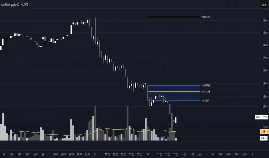
Engulfing DetectorThis script detects classic candlestick reversal patterns known as Engulfing formations:
Bullish Engulfing: A green candle fully engulfs the previous red candle.
Bearish Engulfing: A red candle fully engulfs the previous green candle.
🔎 Features:
Works on any time frame or instrument.
Optional filter to ignore overly large or irregular candles.
Visual signals on the chart (BE/SE labels).
Built-in alerts for automation or notification.
✅ Recommended usage:
For intraday trading, this indicator performs best on the 5-minute chart of the Nasdaq (NQ) between 9:45 AM and 1:00 PM ET (15:45–19:00 CET).
💡 Suggested trading approach:
Optimized for scalping with short-term trades and small take-profits around +0.10%.
