MSTY-WNTR Rebalancing SignalMSTY-WNTR Rebalancing Signal
## Overview
The **MSTY-WNTR Rebalancing Signal** is a custom TradingView indicator designed to help investors dynamically allocate between two YieldMax ETFs: **MSTY** (YieldMax MSTR Option Income Strategy ETF) and **WNTR** (YieldMax Short MSTR Option Income Strategy ETF). These ETFs are tied to MicroStrategy (MSTR) stock, which is heavily influenced by Bitcoin's price due to MSTR's significant Bitcoin holdings.
MSTY benefits from upward movements in MSTR (and thus Bitcoin) through a covered call strategy that generates income but caps upside potential. WNTR, on the other hand, provides inverse exposure, profiting from MSTR declines but losing in rallies. This indicator uses Bitcoin's momentum and MSTR's relative strength to signal when to hold MSTY (bullish phases), WNTR (bearish phases), or stay neutral, aiming to optimize returns by switching allocations at key turning points.
Inspired by strategies discussed in crypto communities (e.g., X posts analyzing MSTR-linked ETFs), this indicator promotes an active rebalancing approach over a "set and forget" buy-and-hold strategy. In simulated backtests over the past 12 months (as of August 4, 2025), the optimized version has shown potential to outperform holding 100% MSTY or 100% WNTR alone, with an illustrative APY of ~125% vs. ~6% for MSTY and ~-15% for WNTR in one scenario.
**Important Disclaimer**: This is not financial advice. Past performance does not guarantee future results. Always consult a financial advisor. Trading involves risk, and you could lose money. The indicator is for educational and informational purposes only.
## Key Features
- **Momentum-Based Signals**: Uses a Simple Moving Average (SMA) on Bitcoin's price to detect bullish (price > SMA) or bearish (price < SMA) trends.
- **RSI Confirmation**: Incorporates MSTR's Relative Strength Index (RSI) to filter signals, avoiding overbought conditions for MSTY and oversold for WNTR.
- **Visual Cues**:
- Green upward triangle for "Hold MSTY".
- Red downward triangle for "Hold WNTR".
- Yellow cross for "Switch" signals.
- Background color: Green for MSTY, red for WNTR.
- **Information Panel**: A table in the top-right corner displays real-time data: BTC Price, SMA value, MSTR RSI, and current Allocation (MSTY, WNTR, or Neutral).
- **Alerts**: Configurable alerts for holding MSTY, holding WNTR, or switching.
- **Optimized Parameters**: Defaults are tuned (SMA: 10 days, RSI: 15 periods, Overbought: 80, Oversold: 20) based on simulations to reduce whipsaws and capture trends effectively.
## How It Works
The indicator's logic is straightforward yet effective for volatile assets like Bitcoin and MSTR:
1. **Primary Trigger (Bitcoin Momentum)**:
- Calculate the SMA of Bitcoin's closing price (default: 10-day).
- Bullish: Current BTC price > SMA → Potential MSTY hold.
- Bearish: Current BTC price < SMA → Potential WNTR hold.
2. **Secondary Filter (MSTR RSI Confirmation)**:
- Compute RSI on MSTR stock (default: 15-period).
- For bullish signals: If RSI > Overbought (80), signal Neutral (avoid overextended rallies).
- For bearish signals: If RSI < Oversold (20), signal Neutral (avoid capitulation bottoms).
3. **Allocation Rules**:
- Hold 100% MSTY if bullish and not overbought.
- Hold 100% WNTR if bearish and not oversold.
- Neutral otherwise (e.g., during choppy or extreme markets) – consider holding cash or avoiding trades.
4. **Rebalancing**:
- Switch signals trigger when the hold changes (e.g., from MSTY to WNTR).
- Recommended frequency: Weekly reviews or on 5% BTC moves to minimize trading costs (aim for 4-6 trades/year).
This approach leverages Bitcoin's influence on MSTR while mitigating the risks of MSTY's covered call drag during downtrends and WNTR's losses in uptrends.
## Setup and Usage
1. **Chart Requirements**:
- Apply this indicator to a Bitcoin chart (e.g., BTCUSD on Binance or Coinbase, daily timeframe recommended).
- Ensure MSTR stock data is accessible (TradingView supports it natively).
2. **Adding to TradingView**:
- Open the Pine Editor.
- Paste the script code.
- Save and add to your chart.
- Customize inputs if needed (e.g., adjust SMA/RSI lengths for different timeframes).
3. **Interpretation**:
- **Green Background/Triangle**: Allocate 100% to MSTY – Bitcoin is in an uptrend, MSTR not overbought.
- **Red Background/Triangle**: Allocate 100% to WNTR – Bitcoin in downtrend, MSTR not oversold.
- **Yellow Switch Cross**: Rebalance your portfolio immediately.
- **Neutral (No Signal)**: Panel shows "Neutral" – Hold cash or previous position; reassess weekly.
- Monitor the panel for key metrics to validate signals manually.
4. **Backtesting and Strategy Integration**:
- Convert to a strategy script by changing `indicator()` to `strategy()` and adding entry/exit logic for automated testing.
- In simulations (e.g., using Python or TradingView's backtester), it has outperformed buy-and-hold in volatile markets by ~100-200% relative APY, but results vary.
- Factor in fees: ETF expense ratios (~0.99%), trading commissions (~$0.40/trade), and slippage.
5. **Risk Management**:
- Use with a diversified portfolio; never allocate more than you can afford to lose.
- Add stop-losses (e.g., 10% trailing) to protect against extreme moves.
- Rebalance sparingly to avoid over-trading in sideways markets.
- Dividends: Reinvest MSTY/WNTR payouts into the current hold for compounding.
## Performance Insights (Simulated as of August 4, 2025)
Based on synthetic backtests modeling the last 12 months:
- **Optimized Strategy APY**: ~125% (by timing switches effectively).
- **Hold 100% MSTY APY**: ~6% (gains from BTC rallies offset by downtrends).
- **Hold 100% WNTR APY**: ~-15% (losses in bull phases outweigh bear gains).
In one scenario with stronger volatility, the strategy achieved ~4533% APY vs. 10% for MSTY and -34% for WNTR, highlighting its potential in dynamic markets. However, these are illustrative; real results depend on actual BTC/MSTR movements. Test thoroughly on historical data.
## Limitations and Considerations
- **Data Dependency**: Relies on accurate BTC and MSTR data; delays or gaps can affect signals.
- **Market Risks**: Bitcoin's volatility can lead to false signals (whipsaws); the RSI filter helps but isn't perfect.
- **No Guarantees**: This indicator doesn't predict the future. MSTR's correlation to BTC may change (e.g., due to regulatory events).
- **Not for All Users**: Best for intermediate/advanced traders familiar with ETFs and crypto. Beginners should paper trade first.
- **Updates**: As of August 4, 2025, this is version 1.0. Future updates may include volume filters or EMA options.
If you find this indicator useful, consider leaving a like or comment on TradingView. Feedback welcome for improvements!
Cari dalam skrip untuk "股票开盘前15分钟交易规则"

ATR % Line from LoD/HoDATR % Line Trading Indicator - Entry Filter Tool
This Pine Script creates a sophisticated ATR (Average True Range) percentage-based entry filter indicator for TradingView that helps traders avoid buying overextended stocks and identify optimal entry zones based on volatility.
Core Functionality - Entry Discipline
The script calculates a maximum entry threshold by taking a percentage of the Average True Range (ATR) and projecting it from the current day's low. This creates a dynamic "no-buy zone" that adapts to market volatility, helping traders avoid purchasing stocks that have already moved too far from their daily base.
Key Calculation:
Measures the ATR over a specified period (default: 14 bars)
Takes a user-defined percentage of that ATR (default: 25%)
Projects this distance from the day's low to establish a maximum entry threshold
Entry Rule: Avoid buying when price exceeds this ATR% level from the daily low or high.
Visual Features
Entry Threshold Line:
Draws a horizontal line at the calculated maximum entry level
Line extends forward for clear visualization of the "no-buy zone"
Red zones above this line indicate overextended conditions
Fully customizable appearance with color, width, and style options
Smart Entry Alerts:
Optional labels show the ATR percentage threshold and exact price level
Visual confirmation when stocks are trading in acceptable entry zones vs. extended areas
Real-Time Monitoring Table:
Displays current distance from daily low as ATR percentage
Shows whether current price is in "safe entry zone" or "extended territory"
Customizable display options for clean chart analysis
Practical Applications for Entry Management
Avoiding Extended Entries:
Primary Use: Don't initiate long positions when price is more than X% ATR from the daily low
Prevents buying stocks that have already made their daily move
Reduces risk of buying at temporary tops within the trading session
Entry Zone Identification:
Price trading below the ATR% line = potential entry opportunity
Price trading above the ATR% line = wait for pullback or skip the trade
Combines volatility analysis with momentum discipline
Risk Management Benefits:
Improved Entry Timing: Enter closer to daily support levels
Better Risk/Reward: Shorter distance to stop loss (daily low)
Reduced Chasing: Systematic approach prevents FOMO-driven entries
Volatility Awareness: Higher volatility stocks get wider acceptable entry ranges
Configuration for Entry Filtering
Key Settings for Entry Management:
ATR Percentage: Set your maximum acceptable extension (15-30% common for day trading)
Reference Point: Use "Low" to measure extension from daily base
Line Style: Make highly visible to clearly see entry threshold
Alert Integration: Visual confirmation of entry-friendly zones
Typical Usage Scenarios:
Conservative Entries: 15-20% ATR from daily low
Moderate Extensions: 25-35% ATR for stronger momentum plays
Aggressive Setups: 40%+ ATR for breakout situations (use with caution)
Entry Strategy Integration
Pre-Market Planning:
Set ATR% threshold based on stock's typical volatility
Identify key levels where entries become unfavorable
Plan alternative entry strategies for extended stocks
Intraday Execution:
Monitor real-time ATR% extension from daily low
Avoid new long positions when threshold is exceeded
Wait for pullbacks to re-enter acceptable entry zones
This tool transforms volatility analysis into practical entry discipline, helping traders maintain consistent entry standards and avoid the costly mistake of chasing overextended stocks. By respecting ATR-based extension limits, traders can improve their entry timing and overall trade profitability.

Range Filter Strategy [Real Backtest]Range Filter Strategy - Real Backtesting
# Overview
Advanced Range Filter strategy designed for realistic backtesting with precise execution timing and comprehensive risk management. Built specifically for cryptocurrency markets with customizable parameters for different assets and timeframes.
Core Algorithm
Range Filter Technology:
- Smooth Average Range calculation using dual EMA filtering
- Dynamic range-based price filtering to identify trend direction
- Anti-noise filtering system to reduce false signals
- Directional momentum tracking with upward/downward counters
Key Features
Real-Time Execution (No Delay)
- Process orders on tick: Immediate execution without waiting for bar close
- Bar magnifier integration for intrabar precision
- Calculate on every tick for maximum responsiveness
- Standard OHLC bypass for enhanced accuracy
Realistic Price Simulation
- HL2 entry pricing (High+Low)/2 for realistic fills
- Configurable spread buffer simulation
- Random slippage generation (0 to max slippage)
- Market liquidity validation before entry
Advanced Signal Filtering
- Volume-based filtering with customizable ratio
- Optional signal confirmation system (1-3 bars)
- Anti-repetition logic to prevent duplicate signals
- Daily trade limit controls
Risk Management
- Fixed Risk:Reward ratios with precise point calculation
- Automatic stop loss and take profit execution
- Position size management
- Maximum daily trades limitation
Alert System
- Real-time alerts synchronized with strategy execution
- Multiple alert types: Setup, Entry, Exit, Status
- Customizable message formatting with price/time inclusion
- TradingView alert panel integration
Default Parameters
Optimized for BTC 5-minute charts:
- Sampling Period: 100
- Range Multiplier: 3.0
- Risk: 50 points
- Reward: 100 points (1:2 R:R)
- Spread Buffer: 2.0 points
- Max Slippage: 1.0 points
Signal Logic
Long Entry Conditions:
- Price above Range Filter line
- Upward momentum confirmed
- Volume requirements met (if enabled)
- Confirmation period completed (if enabled)
- Daily trade limit not exceeded
Short Entry Conditions:
- Price below Range Filter line
- Downward momentum confirmed
- Volume requirements met (if enabled)
- Confirmation period completed (if enabled)
- Daily trade limit not exceeded
Visual Elements
- Range Filter line with directional coloring
- Upper and lower target bands
- Entry signal markers
- Risk/Reward ratio boxes
- Real-time settings dashboard
Customization Options
Market Adaptation:
- Adjust Sampling Period for different timeframes
- Modify Range Multiplier for various volatility levels
- Configure spread/slippage for different brokers
- Set appropriate R:R ratios for trading style
Filtering Controls:
- Enable/disable volume filtering
- Adjust confirmation requirements
- Set daily trade limits
- Customize alert preferences
Performance Features
- Realistic backtesting results aligned with live trading
- Elimination of look-ahead bias
- Proper order execution simulation
- Comprehensive trade statistics
Alert Configuration
Alert Types Available:
- Entry signals with complete trade information
- Setup alerts for early preparation
- Exit notifications for position management
- Filter direction changes for market context
Message Format:
Symbol - Action | Price: XX.XX | Stop: XX.XX | Target: XX.XX | Time: HH:MM
Usage Recommendations
Optimal Settings:
- Bitcoin/Major Crypto: Default parameters
- Forex: Reduce sampling period to 50-70, multiplier to 2.0-2.5
- Stocks: Reduce sampling period to 30-50, multiplier to 1.0-1.8
- Gold: Sampling period 60-80, multiplier 1.5-2.0
TradingView Configuration:
- Recalculate: "On every tick"
- Orders: "Use bar magnifier"
- Data: Real-time feed recommended
Risk Disclaimer
This strategy is designed for educational and analytical purposes. Past performance does not guarantee future results. Always test thoroughly on paper trading before live implementation. Consider market conditions, broker execution, and personal risk tolerance when using any automated trading system.
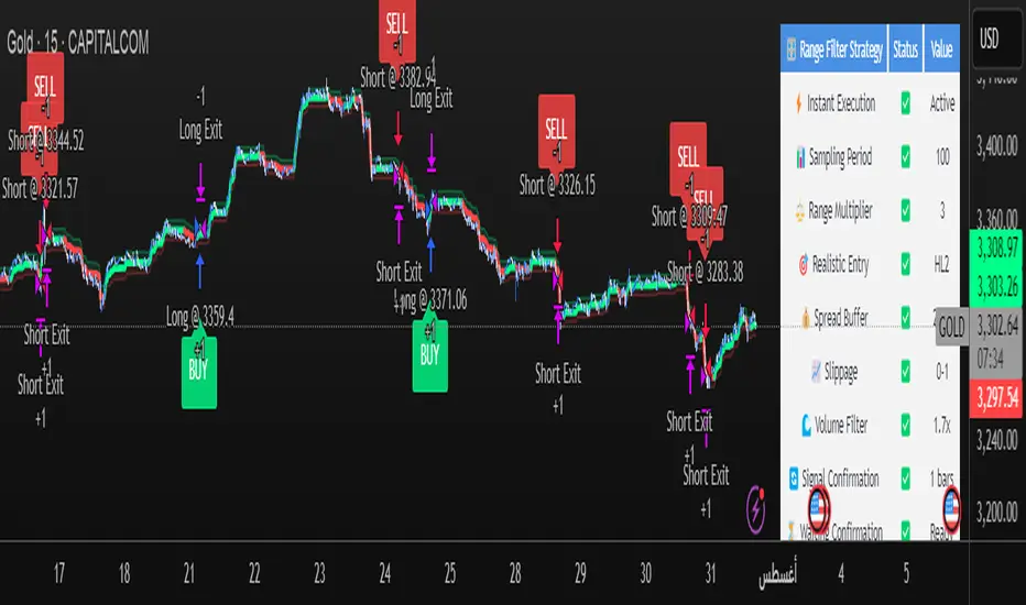
Best Settings Found for Gold 15-Minute Timeframe
After extensive testing and optimization, these are the most effective settings I've discovered for trading Gold (XAUUSD) on the 15-minute timeframe:
Core Filter Settings:
Sampling Period: 100
Range Multiplier: 3.0
Professional Execution Engine:
Realistic Entry: Enabled (HL2)
Spread Buffer: 2 points
Dynamic Slippage: Enabled with max 1 point
Volume Filter: Enabled at 1.7x ratio
Signal Confirmation: Enabled with 1 bar confirmation
Risk Management:
Stop Loss: 50 points
Take Profit: 100 points (2:1 Risk-Reward)
Max Trades Per Day: 5
These settings provide an excellent balance between signal accuracy and realistic market execution. The volume filter at 1.7x ensures we only trade during periods of sufficient market activity, while the 1-bar confirmation helps filter out false signals. The spread buffer and slippage settings account for real trading costs, making backtest results more realistic and achievable in live trading.
Opening-Range BreakoutNote: Default trading date range looks mediocre. Set date range to "Entire History" to see full effect of the strategy. 50.91% profitable trades, 1.178 profit factor, steady profits and limited drawdown. Total P&L: $154,141.18, Max Drawdown: $18,624.36. High R^2
█ Overview
The Opening-Range Breakout strategy is a mechanical, session‑based day‑trading system designed to capture the initial burst of directional momentum immediately following the market open. It defines a user‑configurable “opening range” window, measures its high and low boundaries, then places breakout stop orders at those levels once the range closes. Built‑in filters on minimum range width, reward‑to‑risk ratios, and optional reversal logic help refine entries and manage risk dynamically.
█ How It Works
Opening‑Range Formation
Between 9:30–10:15 AM ET (configurable), the script tracks the highest high and lowest low to form the day’s opening range box.
On the first bar after the range window closes, the range high (OR_high) and low (OR_low) are “locked in.”
Range‑Width Filter
To avoid false breakouts in low‑volatility mornings, the range must be at least X% of the current price (default 0.35%).
If the measured opening-range width < minimum threshold, no orders are placed that day.
Entry & Order Placement
Long: a stop‑buy order at the opening‑range high.
Short: a stop‑sell order at the opening‑range low.
Only one side can trigger (or both if reverse logic is enabled after a losing trade).
Risk Management
Once triggered, each trade uses an ATR‑style stop-loss defined as a percentage retracement of the range (default 50% of range width).
Profit target is set at a configurable Reward/Risk Ratio (default 1.1×).
Optional: Reverse on Stop‑Loss – if the initial breakout loses, immediately reverse into the opposite side on the same day.
Session Exit
Any open positions are closed at the end of the regular trading day (default 3:45 PM ET window end, with hard flat at session close).
Visual cues are provided via green (range high) and red (range low) step‑line plots directly on the chart, allowing you to see the range box and breakout triggers in real time.
█ Why It Works
Early Momentum Capture: The first 15 – 60 minutes of trading encapsulate overnight news digestion and institutional order flow, creating a well‑defined volatility “range.”
Mechanical Discipline: Clear, rule‑based entries and exits remove emotional guesswork, ensuring consistency.
Volatility Filtering: By requiring a minimum range width, the system avoids choppy, low‑range days where false breakouts are common.
Dynamic Sizing: Stops and targets scale with the opening range, adapting automatically to each day’s volatility environment.
█ How to Use
Set Your Instruments & Timeframe
-Apply to any futures contract on a 1‑ to 5‑minute chart.
-Ensure chart timezone is set to America/New_York.
Configure Inputs
-Opening‑Range Window: e.g. “0930-1015” for a 45‑minute range.
-Min. OR Width (%): e.g. 0.35 for 0.35% of current price.
-Reward/Risk Ratio: e.g. 1.1 for a modest profit target above your stop.
-Max OR Retracement %: e.g. 50 to set stop at 50% of range width.
-One Trade Per Day: toggle to limit to a single breakout.
-Reverse on Stop Loss: toggle to flip direction after a losing breakout.
Monitor the Chart
-Watch the green and red range boundaries form during the session open.
-Orders will automatically submit on the first bar after the range window closes, conditioned on your filters.
Review & Adjust
-Backtest across multiple months to validate performance on your preferred contract.
-Tweak range duration, minimum width, and R/R multiple to fit your risk tolerance and desired win‑rate vs. expectancy balance.
█ Settings Reference
Input Defaults
Opening‑Range Window - Time window to form OR (HHMM-HHMM) - 0930–1015
Regular Trading Day - Full session for EOD flat (HHMM-HHMM) - 0930–1545
Min. OR Width (%) - Minimum OR size as % of close to trigger orders - 0.35
Reward/Risk Ratio - Profit target multiple of stop‑loss distance - 1.1
Max OR Retracement (%) - % of OR width to use as stop‑loss distance - 50
One Trade Per Day - Limit to a single breakout order per day - false
Reverse on Stop Loss - Reverse direction immediately after a losing trade - true
Disclaimer
This strategy description and any accompanying code are provided for educational purposes only and do not constitute financial advice or a solicitation to trade. Futures trading involves substantial risk, including possible loss of capital. Past performance is not indicative of future results. Traders should assess their own risk tolerance and conduct thorough backtesting and forward-testing before committing real capital.

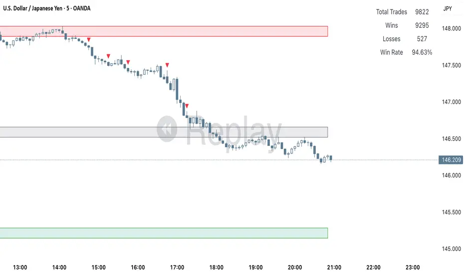
Clarix 5m Scalping Breakout StrategyPurpose
A 5-minute scalping breakout strategy designed to capture fast 3-5 pip moves, using premium/discount zone filters and market bias conditions.
How It Works
The script monitors price action in 5-minute intervals, forming a 15-minute high and low range by tracking the highs and lows of the first 3 consecutive 5-minute candles starting from a custom time. In the next 3 candles, it waits for a breakout above the 15m high or below the 15m low while confirming market bias using custom equilibrium zones.
Buy signals trigger when price breaks the 15m high while in a discount zone
Sell signals trigger when price breaks the 15m low while in a premium zone
The strategy simulates trades with fixed 3-5 pip take profit and stop loss values (configurable). All trades are recorded in a backtest table with live trade results and an automatically updated win rate.
Features
Designed exclusively for the 5-minute timeframe
Custom 15-minute high/low breakout logic
Premium, Discount, and Equilibrium zone display
Built-in backtest tracker with live trade results, statistics, and win rate
Customizable start time, take profit, and stop loss settings
Real-time alerts on breakout signals
Visual markers for trade entries and failed trades
Consistent win rate exceeding 90–95% on average when following market conditions
Usage Tips
Use strictly on 5-minute charts for accurate signal performance. Avoid during high-impact news releases.
Important: Once a trade is opened, manually set your take profit at +3 to +5 pips immediately to secure the move, as these quick scalps often hit the target within a single candle. This prevents missed exits during rapid price action.
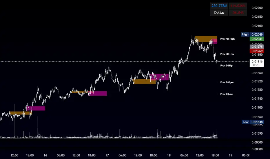
OBR 15min Session Opening Range Breakout + Volume Trend DeltaQuick Overview
This Pine Script plots the opening range for London and New York sessions, highlights breakout levels, draws previous session pivots, and offers a live volume delta table for trend confirmation.
Session Opening Range
- Captures the high/low of the first 15 minutes (configurable) for both London & NY sessions.
- Fills the range area with adjustable semi‑transparent colors.
- Optional alerts fire on breakout above the high or below the low.
Previous Session Levels
- Automatically draws previous day’s High, Low, Open and previous 4‑hour High/Low.
- Helps identify key S/R zones as price approaches ORB breakouts.
Volume Trend Delta
- Uses a CMO‑weighted moving average and ATR bands to detect trend state.
- Accumulates bullish vs. bearish volume during each trend.
- Displays Bull Vol, Bear Vol, and Delta % in a movable table for quick strength checks.
How to Use
1. Let the opening range complete (first 15 min).
2. Look for price closing above/below the ORB—enter long on an upside break, short on a downside break.
3. Check the Volume Delta table: positive delta confirms buying strength; negative delta confirms selling pressure.
4. Use previous day/4h levels as additional support/resistance filters.
Settings & Customization
- ORB Duration & Session Times (London/NY), fill colors, and toggles.
- Enable/disable Previous Day & 4H levels.
- Trend Period, Momentum Window, and Delta table position/size.
- Pre‑built alert conditions for all ORB breakouts.
Developer Notes
- Fully commented for easy adjustments.
- Modular sections: ORB, previous levels, trend delta, and alerts.
- No external libraries—pure Pine Script v6.
Tip
Combine ORB breakouts with Volume Delta and prior session pivots to filter false signals and trade stronger, more reliable moves.
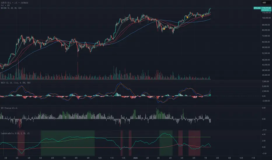
Exponential-Decay Cumulative Spread (Cycle-Tuned)## Indicator Overview
**Exponential-Decay Cumulative Spread (Cycle-Tuned)** – short title **LambdaCumDelta** – tracks the percentage spread between CEXs BTC spot prices.
By clipping outliers, applying an exponential-decay running sum, and comparing that sum to rolling percentile bands, the script flags potential **cycle bottoms** and **cycle tops** whenever the cumulative spread stays beyond extreme thresholds for three consecutive bars.
---
### Core Logic
1. **Price Spread**
`spread_pct = (cexA – cexB) / cexB × 100`.
2. **Outlier Suppression**
* Calculates the **90-day standard deviation σ** of `spread_pct`.
* Uses a **clip coefficient `k_clip`** (0.5–5.0) to cap the spread at `±k_clip × σ`, damping single-day anomalies.
3. **Exponential-Decay Sum**
* Applies a decay factor **λ** (0.50–0.999):
```
CumΔₜ = spread_clipₜ + λ × CumΔₜ₋₁
```
* Larger λ → longer memory half-life.
4. **Rolling Percentile Bands**
* Uses a **365-bar window** to derive dynamic percentile thresholds.
* Upper / Lower bands are set by **perc\_hi** and **perc\_lo** (e.g., 85 % and 15 %).
5. **Signal Definition**
* **Bullish** (cycle bottom): `CumΔ` above the upper band for **3 straight bars**.
* **Bearish** (cycle top): `CumΔ` below the lower band for **3 straight bars**.
---
### Chart Elements
| Plot | Style | Meaning |
| --------------- | ----------------- | ----------------------------------- |
| **CumΔ** | Teal thick line | Exponential-decay cumulative spread |
| Upper Threshold | Green thin line | Rolling upper percentile |
| Lower Threshold | Red thin line | Rolling lower percentile |
| Background | Faded green / red | Bullish / bearish signal zone |
---
### Key Inputs
| Input | Default | Purpose |
| -------------------- | ------- | ------------------------------- |
| **Decay factor λ** | 0.95 | Memory length of CumΔ |
| **Clip coefficient** | 2.0 | Multiple of σ for outlier cap |
| **Upper percentile** | 85 | Cycle-bottom trigger percentile |
| **Lower percentile** | 15 | Cycle-top trigger percentile |
---
### Practical Tips
1. **Timing bias**
* Green background often precedes mean-reversion of the spread – consider scaling into longs or covering shorts.
* Red background suggests stretched positive spread – consider trimming longs or lightening exposure.
2. **Combine with volume, trend filters (MA, MACD, etc.)** to weed out false extremes.
3. Designed for **daily charts**; ensure both exchange feeds are synchronized.
---
### Alerts
Two built-in `alertcondition`s fire when bullish or bearish criteria are met, enabling push / email / webhook notifications.
---
### Disclaimer
This script is for educational and research purposes only and is **not** financial advice. Test thoroughly and trade at your own risk.
Pattern Detector [theUltimator5]🎯 Overview
The Pattern Detector is a comprehensive technical analysis indicator that automatically identifies and visualizes multiple pattern types on your charts. Built with advanced ZigZag technology and sophisticated pattern recognition algorithms, this tool helps traders spot high-probability trading opportunities across all timeframes and markets.
✨ Key Features
🔍 Multi-Pattern Detection System
Harmonic Patterns: Butterfly, Gartley, Bat, and Crab patterns with precise Fibonacci ratios
Classic Reversal Patterns: Head & Shoulders and Inverse Head & Shoulders
Double Patterns: Double Tops and Double Bottoms with extreme validation
Wedge Patterns: Rising and Falling Wedges with volume confirmation
📊 Advanced ZigZag Engine
Customizable sensitivity (5-50 levels)
Depth multiplier for multi-timeframe analysis
Real-time pivot detection with noise filtering
Option to display ZigZag lines only for pure price action analysis
🎨 Visualization
Clean pattern lines with distinct color coding
Point labeling system (X, A, B, C, D for harmonics / LS, H, RS for H&S)
Pattern name displays with bullish/bearish direction
Price target projections with arrow indicators
Subtle pattern fills for enhanced visibility
🛠️ Settings & Configuration
Core ZigZag Settings
ZigZag Sensitivity (5-50): Controls pattern detection sensitivity. Lower values detect more patterns but may include noise. Higher values focus on major swings only.
ZigZag Depth Multiplier (1-5): Multiplies sensitivity for deeper analysis. Level 1 = most responsive, Level 5 = major swings only.
Pattern Detection Toggles
Show ZigZag Lines Only: Displays pure ZigZag without pattern detection for price structure analysis
Detect Harmonic Patterns: Enable/disable Fibonacci-based harmonic pattern detection
Detect Head & Shoulders: Toggle classic reversal pattern identification
Detect Double Tops/Bottoms: Enable double pattern detection with extreme validation
Detect Wedge Patterns: Toggle wedge pattern detection with volume confirmation
Display Options
Show Pattern Names: Display pattern names directly on chart (e.g., "Butterfly (Bullish)")
Show Point Labels: Add lettered labels at key pattern points for structure identification
Project Harmonic Targets: Show projected completion points for incomplete harmonic patterns
📈 Pattern Types Explained
Harmonic Patterns 🦋
Advanced Fibonacci-based patterns that provide high-probability reversal signals:
Butterfly: AB=0.786 XA, BC=0.382-0.886 AB, CD=1.618-2.24 BC
Gartley: AB=0.618 XA, BC=0.382-0.886 AB, CD=1.272-1.618 BC
Bat: AB=0.382-0.50 XA, BC=0.382-0.886 AB, CD=1.618-2.24 BC
Crab: AB=0.382-0.618 XA, BC=0.382-0.886 AB, CD=2.24-3.618 BC
Head & Shoulders 👤
Classic three-peak reversal pattern indicating trend exhaustion:
Standard H&S: Bearish reversal at tops
Inverse H&S: Bullish reversal at bottoms
Automatic neckline validation and price target calculation
Double Patterns 📊
Powerful reversal patterns with extreme validation:
Double Top: Two similar highs with valley between (bearish)
Double Bottom: Two similar lows with peak between (bullish)
Includes lookback period validation to ensure patterns are significant extremes
Wedge Patterns 📐
Continuation/reversal patterns with converging trend lines:
Rising Wedge: Converging upward slopes (typically bearish)
Falling Wedge: Converging downward slopes (typically bullish)
Volume confirmation required for increased accuracy
🎯 Trading Applications
Entry Signals
Harmonic Patterns: Enter at point D completion with targets at point A
H&S Patterns: Enter on neckline break with calculated targets
Double Patterns: Enter on support/resistance break with measured moves
Wedge Patterns: Enter on breakout direction with volume confirmation
Risk Management
Use pattern structure for logical stop placement
Pattern invalidation levels provide clear exit rules
Multiple pattern confirmation increases probability
Multi-Timeframe Analysis
Higher ZigZag depth for longer-term patterns
Lower sensitivity for short-term trading patterns
Combine with other timeframes for confluence
⚙️ Optimal Settings
For Day Trading (1m-15m charts)
ZigZag Sensitivity: 5-9
Depth Multiplier: 1-2
Enable all pattern types for maximum opportunities
For Swing Trading (1H-4H charts)
ZigZag Sensitivity: 9-15
Depth Multiplier: 2-3
Focus on harmonic and H&S patterns
For Position Trading (Daily+ charts)
ZigZag Sensitivity: 15-25
Depth Multiplier: 3-5
Emphasize major harmonic and double patterns
🔧 Technical Specifications
Maximum Lookback: 5000 bars for comprehensive analysis
Pattern Overlap Prevention: Intelligent filtering prevents duplicate patterns
Performance Optimized: Efficient algorithms for real-time detection
Volume Integration: Advanced volume analysis for wedge confirmation
Fibonacci Precision: 10% tolerance for harmonic ratio validation
📚 How to Use
Add to Chart: Apply indicator to any timeframe/market
Configure Settings: Adjust sensitivity based on trading style
Enable Patterns: Toggle desired pattern types
Analyze Results: Look for completed patterns with clear structure
Plan Trades: Use price targets and pattern invalidation for trade management
Perfect for both novice and experienced traders seeking systematic pattern recognition with visualization and entry/exit signals.

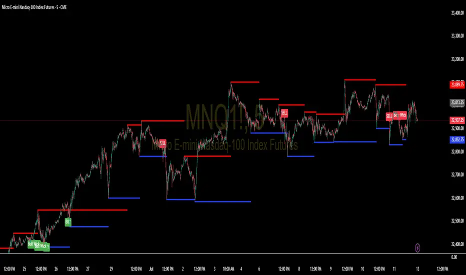
Support and Resistance Levels with BreaksThis indicator identifies dynamic support and resistance levels using pivot point analysis and provides clear trading signals when these levels are broken with volume confirmation. Enhanced version with improved signal clarity for better trading decisions.
## 🔧 Key Features
### Support & Resistance Detection
- Automatically identifies key pivot high and low levels
- Draws clear visual lines (red for resistance, blue for support)
- Configurable sensitivity with left/right bar settings
### Enhanced Trading Signals
- **BUY** signals when resistance is broken with volume confirmation
- **SELL** signals when support is broken with volume confirmation
- **Bull Wick** alerts for potential reversals at resistance
- **Bear Wick** alerts for potential reversals at support
### Volume Confirmation
- Built-in volume oscillator using 5 and 10-period EMAs
- Filters out low-volume false breakouts
- Adjustable volume threshold (default: 20%)
### Complete Alert System
- Support Broken alerts
- Resistance Broken alerts
- Bull Wick reversal alerts
- Bear Wick reversal alerts
## ⚙️ Settings
- **Show Breaks**: Toggle signal display
- **Left Bars**: Pivot detection lookback (default: 15)
- **Right Bars**: Pivot detection lookforward (default: 15)
- **Volume Threshold**: Minimum volume increase for valid signals (default: 20%)
## 📈 Best For
- Swing trading strategies
- Breakout confirmation
- Support/resistance trading
- Volume-based entry signals
## 🔍 How It Works
1. Identifies pivot highs/lows using configurable periods
2. Calculates volume oscillator for confirmation
3. Generates BUY signals on resistance breaks with volume
4. Generates SELL signals on support breaks with volume
5. Detects wick patterns for potential reversals
## 📋 Updates in This Version
- Enhanced BUY/SELL signal clarity (replaced generic "B" labels)
- Added Bull Wick and Bear Wick alert conditions
- Updated to Pine Script v6 compatibility
- Improved signal filtering and accuracy
## ⚠️ Disclaimer
This indicator is for educational and informational purposes only. Always conduct your own analysis and risk management before making trading decisions. Past performance does not guarantee future results.
---
**Original Script**: "Support and Resistance Levels with Breaks" by LuxAlgo
**License**: CC BY-NC-SA 4.0
**Enhanced by**: profitgang
**Version**: Pine Script v6
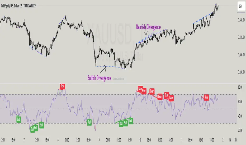
Zero-Lag RSI DivergenceZero-Lag RSI Divergence
Overview
This indicator identifies RSI divergences in real-time without delay, providing immediate signals as price-momentum discrepancies develop. The indicator analyzes price action against RSI momentum across dual configurable periods, enabling traders to detect potential reversal opportunities with zero lag.
Key Features
Instant Divergence Detection : Identifies bullish and bearish divergences immediately upon formation without waiting for candle confirmation or historical validation. This eliminates signal delay but may increase false signals due to higher sensitivity.
Dual Period Analysis : Configure detection across two independent cycles - Short Period (default 15) and Long Period (default 50) - allowing for multi-timeframe divergence analysis and enhanced signal validation across different market conditions.
Visual Divergence Lines : Automatically draws dashed lines connecting divergence points between price highs/lows and corresponding RSI peaks/troughs, clearly illustrating the momentum-price relationship.
Customizable RSI Parameters : Adjustable RSI length (default 14) allows optimization for different market volatility and trading timeframes.
How It Works
The indicator continuously monitors price action patterns and RSI momentum:
- Bullish Divergence : Detected when price makes lower lows while RSI makes higher lows, suggesting potential upward momentum
- Bearish Divergence : Identified when price makes higher highs while RSI makes lower highs, indicating potential downward momentum
The algorithm uses candle color transitions and immediate RSI comparisons to trigger signals without historical repainting , ensuring backtesting accuracy and real-time reliability.
How To Read
Important Notes
Higher Signal Frequency : The zero-lag approach increases signal sensitivity, generating more frequent alerts that may include false signals. Consider using additional confirmation methods for trade entries.
Non-Repainting : All signals are generated and maintained without historical modification, ensuring consistent backtesting and forward-testing results.
Input Parameters
RSI Length: Period for RSI calculation (default: 14)
Short/Long Periods: Lookback periods for divergence detection (default: 15/50)
Line Colors: Customizable colors for short and long period divergence lines
Label Settings: Optional divergence labels with custom text
This indicator is designed for traders seeking immediate divergence identification across multiple timeframes while maintaining signal integrity and backtesting reliability.
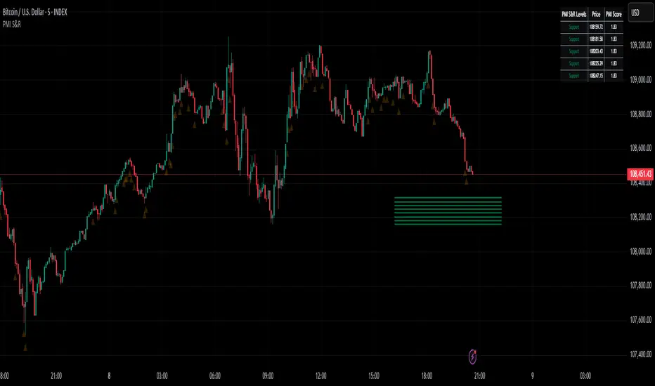
Active PMI Support/Resistance Levels [EdgeTerminal]The PMI Support & Resistance indicator revolutionizes traditional technical analysis by using Pointwise Mutual Information (PMI) - a statistical measure from information theory - to objectively identify support and resistance levels. Unlike conventional methods that rely on visual pattern recognition, this indicator provides mathematically rigorous, quantifiable evidence of price levels where significant market activity occurs.
- The Mathematical Foundation: Pointwise Mutual Information
Pointwise Mutual Information measures how much more likely two events are to occur together compared to if they were statistically independent. In our context:
Event A: Volume spikes occurring (high trading activity)
Event B: Price being at specific levels
The PMI formula calculates: PMI = log(P(A,B) / (P(A) × P(B)))
Where:
P(A,B) = Probability of volume spikes occurring at specific price levels
P(A) = Probability of volume spikes occurring anywhere
P(B) = Probability of price being at specific levels
High PMI scores indicate that volume spikes and certain price levels co-occur much more frequently than random chance would predict, revealing genuine support and resistance zones.
- Why PMI Outperforms Traditional Methods
Subjective interpretation: What one trader sees as significant, another might ignore
Confirmation bias: Tendency to see patterns that confirm existing beliefs
Inconsistent criteria: No standardized definition of "significant" volume or price action
Static analysis: Doesn't adapt to changing market conditions
No strength measurement: Can't quantify how "strong" a level truly is
PMI Advantages:
✅ Objective & Quantifiable: Mathematical proof of significance, not visual guesswork
✅ Statistical Rigor: Levels backed by information theory and probability
✅ Strength Scoring: PMI scores rank levels by statistical significance
✅ Adaptive: Automatically adjusts to different market volatility regimes
✅ Eliminates Bias: Computer-calculated, removing human interpretation errors
✅ Market Structure Aware: Reveals the underlying order flow concentrations
- How It Works
Data Processing Pipeline:
Volume Analysis: Identifies volume spikes using configurable thresholds
Price Binning: Divides price range into discrete levels for analysis
Co-occurrence Calculation: Measures how often volume spikes happen at each price level
PMI Computation: Calculates statistical significance for each price level
Level Filtering: Shows only levels exceeding minimum PMI thresholds
Dynamic Updates: Refreshes levels periodically while maintaining historical traces
Visual System:
Current Levels: Bright, thick lines with PMI scores - your actionable levels
Historical Traces: Faded previous levels showing market structure evolution
Strength Tiers: Line styles indicate PMI strength (solid/dashed/dotted)
Color Coding: Green for support, red for resistance
Info Table: Real-time display of strongest levels with scores
- Indicator Settings:
Core Parameters
Lookback Period (Default: 200)
Lower (50-100): More responsive to recent price action, catches short-term levels
Higher (300-500): Focuses on major historical levels, more stable but less responsive
Best for: Day trading (100-150), Swing trading (200-300), Position trading (400-500)
Volume Spike Threshold (Default: 1.5)
Lower (1.2-1.4): More sensitive, catches smaller volume increases, more levels detected
Higher (2.0-3.0): Only major volume surges count, fewer but stronger signals
Market dependent: High-volume stocks may need higher thresholds (2.0+), low-volume stocks lower (1.2-1.3)
Price Bins (Default: 50)
Lower (20-30): Broader price zones, less precise but captures wider areas
Higher (70-100): More granular levels, precise but may be overly specific
Volatility dependent: High volatility assets benefit from more bins (70+)
Minimum PMI Score (Default: 0.5)
Lower (0.2-0.4): Shows more levels including weaker ones, comprehensive view
Higher (1.0-2.0): Only statistically strong levels, cleaner chart
Progressive filtering: Start with 0.5, increase if too cluttered
Max Levels to Show (Default: 8)
Fewer (3-5): Clean chart focusing on strongest levels only
More (10-15): Comprehensive view but may clutter chart
Strategy dependent: Scalpers prefer fewer (3-5), swing traders more (8-12)
Historical Tracking Settings
Update Frequency (Default: 20 bars)
Lower (5-10): More frequent updates, captures rapid market changes
Higher (50-100): Less frequent updates, focuses on major structural shifts
Timeframe scaling: 1-minute charts need lower frequency (5-10), daily charts higher (50+)
Show Historical Levels (Default: True)
Enables the "breadcrumb trail" effect showing evolution of support/resistance
Disable for cleaner charts focusing only on current levels
Max Historical Marks (Default: 50)
Lower (20-30): Less memory usage, shorter history
Higher (100-200): Longer historical context but more resource intensive
Fade Strength (Default: 0.8)
Lower (0.5-0.6): Historical levels more visible
Higher (0.9-0.95): Historical levels very subtle
Visual Settings
Support/Resistance Colors: Choose colors that contrast well with your chart theme Line Width: Thicker lines (3-4) for better visibility on busy charts Show PMI Scores: Toggle labels showing statistical strength Label Size: Adjust based on screen resolution and chart zoom level
- Most Effective Usage Strategies
For Day Trading:
Setup: Lookback 100-150, Volume Threshold 1.8-2.2, Update Frequency 10-15
Use PMI levels as bounce/rejection points for scalp entries
Higher PMI scores (>1.5) offer better probability setups
Watch for volume spike confirmations at levels
For Swing Trading:
Setup: Lookback 200-300, Volume Threshold 1.5-2.0, Update Frequency 20-30
Enter on pullbacks to high PMI support levels
Target next resistance level with PMI score >1.0
Hold through minor levels, exit at major PMI levels
For Position Trading:
Setup: Lookback 400-500, Volume Threshold 2.0+, Update Frequency 50+
Focus on PMI scores >2.0 for major structural levels
Use for portfolio entry/exit decisions
Combine with fundamental analysis for timing
- Trading Applications:
Entry Strategies:
PMI Bounce Trades
Price approaches high PMI support level (>1.0)
Wait for volume spike confirmation (orange triangles)
Enter long on bullish price action at the level
Stop loss just below the PMI level
Target: Next PMI resistance level
PMI Breakout Trades
Price consolidates near high PMI level
Volume increases (watch for orange triangles)
Enter on decisive break with volume
Previous resistance becomes new support
Target: Next major PMI level
PMI Rejection Trades
Price approaches PMI resistance with momentum
Watch for rejection signals and volume spikes
Enter short on failure to break through
Stop above the PMI level
Target: Next PMI support level
Risk Management:
Stop Loss Placement
Place stops 0.1-0.5% beyond PMI levels (adjust for volatility)
Higher PMI scores warrant tighter stops
Use ATR-based stops for volatile assets
Position Sizing
Larger positions at PMI levels >2.0 (highest conviction)
Smaller positions at PMI levels 0.5-1.0 (lower conviction)
Scale out at multiple PMI targets
- Key Warning Signs & What to Watch For
Red Flags:
🚨 Very Low PMI Scores (<0.3): Weak statistical significance, avoid trading
🚨 No Volume Confirmation: PMI level without recent volume spikes may be stale
🚨 Overcrowded Levels: Too many levels close together suggests poor parameter tuning
🚨 Outdated Levels: Historical traces are reference only, not tradeable
Optimization Tips:
✅ Regular Recalibration: Adjust parameters monthly based on market regime changes
✅ Volume Context: Always check for recent volume activity at PMI levels
✅ Multiple Timeframes: Confirm PMI levels across different timeframes
✅ Market Conditions: Higher thresholds during high volatility periods
Interpreting PMI Scores
PMI Score Ranges:
0.5-1.0: Moderate statistical significance, proceed with caution
1.0-1.5: Good significance, reliable for most trading strategies
1.5-2.0: Strong significance, high-confidence trade setups
2.0+: Very strong significance, institutional-grade levels
Historical Context: The historical trace system shows how support and resistance evolve over time. When current levels align with multiple historical traces, it indicates persistent market memory at those prices, significantly increasing the level's reliability.
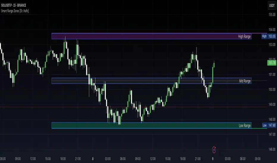
Smart Range Zones [Dr. Hafiz]Smart Range Zones
Description:
This indicator highlights key market zones — High Range, Mid Range, and Low Range — to help traders visually understand dynamic support and resistance levels.
✅ High Range: Potential supply/resistance area
✅ Mid Range: Fair value or equilibrium zone
✅ Low Range: Potential demand/support area
The zones are calculated based on the highest and lowest price over a user-defined period (default: 130 bars) and dynamically projected forward.
🔸 EMA 15 Line is included as an optional trend filter — helping confirm direction or trend alignment.
🔧 Features:
Auto-calculated High/Mid/Low zones
Real-time dynamic projections
Right-aligned zone labels inside each box
Clean visual structure
Toggle for showing/hiding EMA 15
📌 Best suited for:
Intraday & swing traders
Range breakouts and rejections
Trend confirmation with EMA
Created and published by Dr. Hafiz, modified under the MPL 2.0 license.
ITM 2x15// © 2025 Intraday Trading Machine
// This script is open-source. You may use and modify it, but please give credit.
// Colors the current 15-minute candle body green or red if the two previous candles were both bullish or bearish.
This script is designed for traders using the Scalping Intraday Trading Machine technique. It highlights when two consecutive 15-minute candles close in the same direction — either both bullish or both bearish.
For example, if you see two consecutive bearish candles, you might look for a long entry on a break above the high of the first bearish candle. This tool helps you visually identify these setups with clean, directional candle coloring — no clutter.
Custom Daily Session Zones by KoenigseggCustom Daily Session Zones
🟣 Description
This indicator displays customizable trading session time zones as background highlights on your chart, on any timeframe you choose. The inline info tooltip provides the precise start and end times of the three largest market sessions—the US, the EU, and ASIA—for quick reference. It provides flexible control over session times for different days of the week, making it ideal for traders who need to visualize specific market hours or trading sessions.
🟣 Key Features
- Flexible Session Configuration: Set a common session time for all days or customize individual sessions for each day of the week
- Per-Day Control: Enable or disable sessions for specific days (Monday through Sunday)
- Color Customization: Choose unique colors for each day's session zones
- UTC Timezone Standard: All session times are defined in UTC to ensure consistency across charts
- Clean Visual Display: Non-intrusive background highlighting that doesn't interfere with price action
🟣 How to Use
- Common Session Mode: Use the default mode to apply the same session time across all enabled days
- Manual Per-Day Mode: Enable "Manual per-day sessions" to set different session times for each day
- Day Selection: Toggle individual days on/off based on your trading schedule
- Color Coding: Customize colors for each day to easily distinguish between different sessions
🟣 Technical Details
- Uses Pine Script v6 for optimal performance
- Implements proper session time detection using TradingView's built-in time functions
- Operates in UTC timezone for all session calculations
- Lightweight code that doesn't impact chart performance
🟣 Use Cases
- Highlight specific trading sessions (London, New York, Tokyo, etc.)
- Mark important market hours for your trading strategy
- Visualize different session overlaps
- Create custom trading time windows
- Track market activity during specific hours
🟣 Compatibility
- Works on all timeframes
- Compatible with all asset classes (Forex, Stocks, Crypto, Futures, etc.)
- Supports all TradingView chart types
- Responsive design that adapts to different screen sizes
🟣 Image Descriptions
- First Image (main image): Shows multiple New York Stock Exchange sessions from 1:30 p.m. to 8:00 p.m. (UTC), on the 15-minute timeframe, with each day’s zone colored differently to demonstrate the indicator’s customizable color settings.
- Second Image: A zoomed‑in fractal chart view of the same New York session on the 15-minute timeframe, illustrating how the background session zone appears even at higher detail levels.
Third Image: A close‑up of the New York session (1:30 p.m. to 8:00 p.m.) on the 3-minute timeframe, reaffirming the consistency of zone highlighting across different zoom levels.
🟣 Future Updates (v2)
In the next release, you’ll be able to define multiple session blocks per day—displaying two distinct colored zones within the same trading day. This will help you visualize when one market session ends and another begins without losing chart clarity.
🟣 Conclusion
This indicator is perfect for traders who need precise control over Market Session visualization and want to maintain a clean, professional chart appearance.
🟣 Disclaimer
This script is provided for educational and illustrative purposes only. It is not financial or trading advice, nor a recommendation to buy or sell any asset. Always conduct your own research and consult a professional before making any trading decisions.

Simple Market Kill-Zones + Open (UTC)What it does
This Pine v6 indicator highlights the “kill-zones” around the big session opens—Asian (23:00–03:00 UTC), London (07:00–09:00 UTC) and New York (13:30–15:30 UTC)—by reading each bar’s actual UTC timestamp. It also draws dashed vertical lines at exactly 23:00, 07:00 and 13:30 UTC, so you never miss the liquidity ramps. Because it uses raw UTC hours/minutes, it stays accurate even when exchanges pause (e.g. Nano-BTC’s daily halt) or your chart’s display timezone changes.
Key Inputs
Show Asia/London/NY Kill Zone – toggle each shaded band on/off
Zone Colors – pick your own semi-transparent hues
Show Session-Open Lines – enable dashed verticals at the exact open times
Line Colors – customize the line opacity and style
How to use
Apply on your favorite timeframe (15 min–1 h is a sweet spot).
Toggle the zones you care about and pick readable colors.
Use the dashed lines as entry triggers or as visual bookmarks.
In your own Pine strategies, wrap order logic with the zone booleans to only trade when liquidity’s alive.
Intraday Session Levels: Pre-Mkt, 5m, 15m (Replay/Toggle/Labels)Intraday Session Levels: Pre-Mkt, 5m, 15m (Replay/Toggle/Labels)
Version v1.0
Live session levels for every trader!
This indicator automatically tracks and draws the most actionable intraday levels as they develop—live in real-time and fully compatible with TradingView’s bar replay and backtesting.
How it works:
Pre-Market High & Low:
Levels appear and update live as soon as the pre-market session starts (4:00am ET), then “freeze” at the official open (9:30am ET) and remain visible for the rest of the day.
First 5-Minute Candle High/Low:
Drawn instantly after the first 5-minute candle (9:30–9:35am ET) completes.
First 15-Minute Candle High/Low:
Drawn right after the first 15-minute candle (9:30–9:45am ET) completes.
Labels on every line
Each level is clearly labeled on your chart (“PreMkt High”, “5m Low”, “15m High”, etc).
Perfect for backtesting:
All levels display exactly as they would have appeared in real time, making this indicator fully bar replay and historical test compatible.
Flexible ON/OFF toggles:
Instantly show or hide Pre-Mkt, 5m, and 15m levels via the settings panel.
Why use it?
Identify support/resistance and key reaction zones intraday
Fade or break the opening range with confidence
Backtest your strategies with accurate historical context
Reduce chart clutter with customizable, minimal visuals
Whether you’re a scalper, day trader, or backtest enthusiast, this tool keeps your charts focused and your edge sharp.
Developed by

Session Makers v1
Session Makers v1 - Professional Trading Session Visualizer
This advanced indicator highlights key trading sessions and market structure levels, helping traders identify optimal trading times and important price levels.
Key Features:
Session Time Markers
- Vertical dotted lines at major market opens (London/New York)
- Appears 30 minutes before each session for early preparation
Interactive Session Boxes
- Asia Session (22:00-06:00 GMT) - Blue shaded area
- London AM (08:00-09:00 GMT) - Gray shaded area
- London/New York Overlap (14:00-15:00 GMT) - Gray shaded area
Key Reference Levels
- Yesterday's high/low (with touch alerts)
- Previous week's high/low (with touch alerts)
- Asia session high/low/mid lines
Smart Visual Design
- Clean, non-cluttered visuals that adapt to your chart
- Customizable colors and transparency for all elements
- Optimized for all timeframes (M1-H4)
only use in timeframes <= 15 min
KST Strategy [Skyrexio]Overview
KST Strategy leverages Know Sure Thing (KST) indicator in conjunction with the Williams Alligator and Moving average to obtain the high probability setups. KST is used for for having the high probability to enter in the direction of a current trend when momentum is rising, Alligator is used as a short term trend filter, while Moving average approximates the long term trend and allows trades only in its direction. Also strategy has the additional optional filter on Choppiness Index which does not allow trades if market is choppy, above the user-specified threshold. Strategy has the user specified take profit and stop-loss numbers, but multiplied by Average True Range (ATR) value on the moment when trade is open. The strategy opens only long trades.
Unique Features
ATR based stop-loss and take profit. Instead of fixed take profit and stop-loss percentage strategy utilizes user chosen numbers multiplied by ATR for its calculation.
Configurable Trading Periods. Users can tailor the strategy to specific market windows, adapting to different market conditions.
Optional Choppiness Index filter. Strategy allows to choose if it will use the filter trades with Choppiness Index and set up its threshold.
Methodology
The strategy opens long trade when the following price met the conditions:
Close price is above the Alligator's jaw line
Close price is above the filtering Moving average
KST line of Know Sure Thing indicator shall cross over its signal line (details in justification of methodology)
If the Choppiness Index filter is enabled its value shall be less than user defined threshold
When the long trade is executed algorithm defines the stop-loss level as the low minus user defined number, multiplied by ATR at the trade open candle. Also it defines take profit with close price plus user defined number, multiplied by ATR at the trade open candle. While trade is in progress, if high price on any candle above the calculated take profit level or low price is below the calculated stop loss level, trade is closed.
Strategy settings
In the inputs window user can setup the following strategy settings:
ATR Stop Loss (by default = 1.5, number of ATRs to calculate stop-loss level)
ATR Take Profit (by default = 3.5, number of ATRs to calculate take profit level)
Filter MA Type (by default = Least Squares MA, type of moving average which is used for filter MA)
Filter MA Length (by default = 200, length for filter MA calculation)
Enable Choppiness Index Filter (by default = true, setting to choose the optional filtering using Choppiness index)
Choppiness Index Threshold (by default = 50, Choppiness Index threshold, its value shall be below it to allow trades execution)
Choppiness Index Length (by default = 14, length used in Choppiness index calculation)
KST ROC Length #1 (by default = 10, value used in KST indicator calculation, more information in Justification of Methodology)
KST ROC Length #2 (by default = 15, value used in KST indicator calculation, more information in Justification of Methodology)
KST ROC Length #3 (by default = 20, value used in KST indicator calculation, more information in Justification of Methodology)
KST ROC Length #4 (by default = 30, value used in KST indicator calculation, more information in Justification of Methodology)
KST SMA Length #1 (by default = 10, value used in KST indicator calculation, more information in Justification of Methodology)
KST SMA Length #2 (by default = 10, value used in KST indicator calculation, more information in Justification of Methodology)
KST SMA Length #3 (by default = 10, value used in KST indicator calculation, more information in Justification of Methodology)
KST SMA Length #4 (by default = 15, value used in KST indicator calculation, more information in Justification of Methodology)
KST Signal Line Length (by default = 10, value used in KST indicator calculation, more information in Justification of Methodology)
User can choose the optimal parameters during backtesting on certain price chart.
Justification of Methodology
Before understanding why this particular combination of indicator has been chosen let's briefly explain what is KST, Williams Alligator, Moving Average, ATR and Choppiness Index.
The KST (Know Sure Thing) is a momentum oscillator developed by Martin Pring. It combines multiple Rate of Change (ROC) values, smoothed over different timeframes, to identify trend direction and momentum strength. First of all, what is ROC? ROC (Rate of Change) is a momentum indicator that measures the percentage change in price between the current price and the price a set number of periods ago.
ROC = 100 * (Current Price - Price N Periods Ago) / Price N Periods Ago
In our case N is the KST ROC Length inputs from settings, here we will calculate 4 different ROCs to obtain KST value:
KST = ROC1_smooth × 1 + ROC2_smooth × 2 + ROC3_smooth × 3 + ROC4_smooth × 4
ROC1 = ROC(close, KST ROC Length #1), smoothed by KST SMA Length #1,
ROC2 = ROC(close, KST ROC Length #2), smoothed by KST SMA Length #2,
ROC3 = ROC(close, KST ROC Length #3), smoothed by KST SMA Length #3,
ROC4 = ROC(close, KST ROC Length #4), smoothed by KST SMA Length #4
Also for this indicator the signal line is calculated:
Signal = SMA(KST, KST Signal Line Length)
When the KST line rises, it indicates increasing momentum and suggests that an upward trend may be developing. Conversely, when the KST line declines, it reflects weakening momentum and a potential downward trend. A crossover of the KST line above its signal line is considered a buy signal, while a crossover below the signal line is viewed as a sell signal. If the KST stays above zero, it indicates overall bullish momentum; if it remains below zero, it points to bearish momentum. The KST indicator smooths momentum across multiple timeframes, helping to reduce noise and provide clearer signals for medium- to long-term trends.
Next, let’s discuss the short-term trend filter, which combines the Williams Alligator and Williams Fractals. Williams Alligator
Developed by Bill Williams, the Alligator is a technical indicator that identifies trends and potential market reversals. It consists of three smoothed moving averages:
Jaw (Blue Line): The slowest of the three, based on a 13-period smoothed moving average shifted 8 bars ahead.
Teeth (Red Line): The medium-speed line, derived from an 8-period smoothed moving average shifted 5 bars forward.
Lips (Green Line): The fastest line, calculated using a 5-period smoothed moving average shifted 3 bars forward.
When the lines diverge and align in order, the "Alligator" is "awake," signaling a strong trend. When the lines overlap or intertwine, the "Alligator" is "asleep," indicating a range-bound or sideways market. This indicator helps traders determine when to enter or avoid trades.
The next indicator is Moving Average. It has a lot of different types which can be chosen to filter trades and the Least Squares MA is used by default settings. Let's briefly explain what is it.
The Least Squares Moving Average (LSMA) — also known as Linear Regression Moving Average — is a trend-following indicator that uses the least squares method to fit a straight line to the price data over a given period, then plots the value of that line at the most recent point. It draws the best-fitting straight line through the past N prices (using linear regression), and then takes the endpoint of that line as the value of the moving average for that bar. The LSMA aims to reduce lag and highlight the current trend more accurately than traditional moving averages like SMA or EMA.
Key Features:
It reacts faster to price changes than most moving averages.
It is smoother and less noisy than short-term EMAs.
It can be used to identify trend direction, momentum, and potential reversal points.
ATR (Average True Range) is a volatility indicator that measures how much an asset typically moves during a given period. It was introduced by J. Welles Wilder and is widely used to assess market volatility, not direction.
To calculate it first of all we need to get True Range (TR), this is the greatest value among:
High - Low
abs(High - Previous Close)
abs(Low - Previous Close)
ATR = MA(TR, n) , where n is number of periods for moving average, in our case equals 14.
ATR shows how much an asset moves on average per candle/bar. A higher ATR means more volatility; a lower ATR means a calmer market.
The Choppiness Index is a technical indicator that quantifies whether the market is trending or choppy (sideways). It doesn't indicate trend direction — only the strength or weakness of a trend. Higher Choppiness Index usually approximates the sideways market, while its low value tells us that there is a high probability of a trend.
Choppiness Index = 100 × log10(ΣATR(n) / (MaxHigh(n) - MinLow(n))) / log10(n)
where:
ΣATR(n) = sum of the Average True Range over n periods
MaxHigh(n) = highest high over n periods
MinLow(n) = lowest low over n periods
log10 = base-10 logarithm
Now let's understand how these indicators work in conjunction and why they were chosen for this strategy. KST indicator approximates current momentum, when it is rising and KST line crosses over the signal line there is high probability that short term trend is reversing to the upside and strategy allows to take part in this potential move. Alligator's jaw (blue) line is used as an approximation of a short term trend, taking trades only above it we want to avoid trading against trend to increase probability that long trade is going to be winning.
Almost the same for Moving Average, but it approximates the long term trend, this is just the additional filter. If we trade in the direction of the long term trend we increase probability that higher risk to reward trade will hit the take profit. Choppiness index is the optional filter, but if it turned on it is used for approximating if now market is in sideways or in trend. On the range bounded market the potential moves are restricted. We want to decrease probability opening trades in such condition avoiding trades if this index is above threshold value.
When trade is open script sets the stop loss and take profit targets. ATR approximates the current volatility, so we can make a decision when to exit a trade based on current market condition, it can increase the probability that strategy will avoid the excessive stop loss hits, but anyway user can setup how many ATRs to use as a stop loss and take profit target. As was said in the Methodology stop loss level is obtained by subtracting number of ATRs from trade opening candle low, while take profit by adding to this candle's close.
Backtest Results
Operating window: Date range of backtests is 2023.01.01 - 2025.05.01. It is chosen to let the strategy to close all opened positions.
Commission and Slippage: Includes a standard Binance commission of 0.1% and accounts for possible slippage over 5 ticks.
Initial capital: 10000 USDT
Percent of capital used in every trade: 60%
Maximum Single Position Loss: -5.53%
Maximum Single Profit: +8.35%
Net Profit: +5175.20 USDT (+51.75%)
Total Trades: 120 (56.67% win rate)
Profit Factor: 1.747
Maximum Accumulated Loss: 1039.89 USDT (-9.1%)
Average Profit per Trade: 43.13 USDT (+0.6%)
Average Trade Duration: 27 hours
These results are obtained with realistic parameters representing trading conditions observed at major exchanges such as Binance and with realistic trading portfolio usage parameters.
How to Use
Add the script to favorites for easy access.
Apply to the desired timeframe and chart (optimal performance observed on 1h BTC/USDT).
Configure settings using the dropdown choice list in the built-in menu.
Set up alerts to automate strategy positions through web hook with the text: {{strategy.order.alert_message}}
Disclaimer:
Educational and informational tool reflecting Skyrexio commitment to informed trading. Past performance does not guarantee future results. Test strategies in a simulated environment before live implementation.
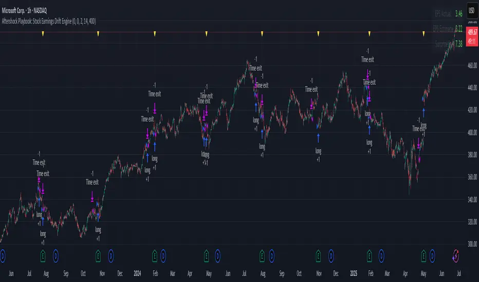
Aftershock Playbook: Stock Earnings Drift EngineStrategy type
Event-driven post-earnings momentum engine (long/short) built for single-stock charts or ADRs that publish quarterly results.
What it does
Detects the exact earnings bar (request.earnings, lookahead_off).
Scores the surprise and launches a position on that candle’s close.
Tracks PnL: if the first leg closes green, the engine automatically re-enters on the very next bar, milking residual drift.
Blocks mid-cycle trades after a loss until the next earnings release—keeping the risk contained to one cycle.
Think of it as a sniper that fires on the earnings pop, reloads once if the shot lands, then goes silent until the next report.
Core signal inputs
Component Default Purpose
EPS Surprise % +0 % / –5 % Minimum positive / negative shock to trigger longs/shorts.
Reverse signals? Off Quick flip for mean-reversion experiments.
Time Risk Mgt. Off Optional hard exit after 45 calendar days (auto-scaled to any TF).
Risk engine
ATR-based stop (ATR × 2 by default, editable).
Bar time stop (15-min → Daily: Have to select the bar value ).
No pyramiding beyond the built-in “double-tap”.
All positions sized as % of equity via Strategy Properties.
Visual aids
Yellow triangle marks the earnings bar.
Diagnostics table (top-right) shows last Actual, Estimate, and Surprise %.
Status-line tool-tips on every input.
Default inputs
Setting Value
Positive surprise ≥ 0 %
Negative surprise ≤ –5 %
ATR stop × 2
ATR length 50
Hold horizon 350 ( 1h timeframe chart bars)
Back-test properties
Initial capital 10 000
Order size 5 % of equity
Pyramiding 1 (internal re-entry only)
Commission 0.03 %
Slippage 5 ticks
Fills Bar magnifier ✔ · On bar close ✔ · Standard OHLC ✔
How to use
Add the script to any earnings-driven stock (AAPL, MSFT, TSLA…).
Turn on Time Risk Management if you want stricter risk management
Back-test different ATR multipliers to fit the stock’s volatility.
Sync commission & slippage with your broker before forward-testing.
Important notes
Works on every timeframe from 15 min to 1 D. Sweet spot around 30min/1h
All request.earnings() & request.security() calls use lookahead_off—zero repaint.
The “double-tap” re-entry occurs once per winning cycle to avoid drift-chasing loops.
Historical stats ≠ future performance. Size positions responsibly.
Simple Sessions & LevelsWhat this indicator does:
This script marks out two essential types of price levels for intraday and swing traders:
The high and low of a customizable 15-minute opening range after the market/session open.
The previous day’s high, midpoint (“halfback”), and low.
How it works:
The script lets you set the session start time (hour and minute) to match your market.
It then calculates the high and low of the first 15 minutes after the session opens and plots those as solid lines.
It also plots the prior day’s high, halfback (midpoint), and low on your chart for easy reference.
Each line and each label can be toggled on or off independently in the settings for maximum customization.
Colors for each level are also fully customizable.
How to use it:
Add the script to your chart.
Set the session start hour and minute to match the open of the market or instrument you trade.
Choose which levels and labels you want displayed by using the toggles in the settings.
The indicator will automatically draw the session range and prior day levels for you.
Use these lines as reference for key support, resistance, and potential trade entry/exit points.
What makes it unique and useful:
This tool combines a flexible session opening range with classic daily reference levels in one package. You have complete control over which levels and labels are shown, making it adaptable for any trading style. It’s especially useful for day traders who want to quickly identify volatility windows and the most important price levels from the previous session.

15m ORB Pip Run with Range HighlightThis marks up the first 15 minute range of the NYSE at 9:30 AM EST.
Then it counts the number of pips that price has run in the direction of the breakout.
The script it not anything amazing.
I just wrote it to help me backtest the 15 minute ORB strategy quickly.

80% Rule Indicator (ETH Session + SVP Prior Session)I created this script to show the 80% opportunity on chart if setting lines up.
"80% rule: Open outside the vah or Val. Spend 30 mins outside there then break back inside spend 15 mins below or above depending which way u broke. Then come back and retest the vah/val and take it to the poc as a first target with the final target being the other Val/vah "
📌 Script Summary
The "80% Rule Indicator (ETH Session + SVP Prior Session)" overlays your chart with prior session value area levels (VAH, VAL, and POC) calculated from extended-hours 30-minute data. It tracks when the price reenters the value area and confirms 80% Rule setups during your chosen trading session. You can optionally trigger alerts, show/hide market sessions, and fine-tune line appearance for a clean, modular workflow.
⚙️ Options & Settings Breakdown
- Use 24-Hour Session (All Markets)
When checked, the indicator ignores time zones and tracks signals during a full 24-hour period (0000-0000), helpful if you're outside U.S. trading hours or want consistent behavior globally.
- Market Session
Dropdown to select one of three key market zones:
- New York (09:30–16:00 ET)
- London (08:00–16:30 local)
- Tokyo (09:00–15:00 local)
Used to gate entry signals during relevant hours unless you choose the 24-hour option.
- Show PD VAH/VAL/POC Lines
Toggle to show or hide prior day’s levels (based on the 30-min extended session). Turning this off removes both the lines and their white text labels.
- Extend Lines Right
When enabled, the VAH/VAL/POC lines extend into the current day’s session. If disabled, they appear only at their anchor point.
- Highlight Selected Session
Adds a soft blue background to help visualize the active session you selected.
- Enable Alert Conditions
Allows TradingView alerts to be created for long/short 80% Rule entries.
- Enable Audible Alerts
Plays an in-chart sound with a popup message (“80% Rule LONG” or “SHORT”) when signals trigger. Requires the chart to be active and sounds enabled in TradingView.

LilSpecCodes1. Killzone Background Highlighting:
It highlights 4 key market sessions:
Killzone Time (EST) Color
Silver Bullet 9:30 AM – 12:00 PM Light Blue
London Killzone 2:00 AM – 5:00 AM Light Green
NY PM Killzone 1:30 PM – 4:00 PM Light Purple
Asia Open 7:00 PM – 11:00 PM Light Red
These are meant to help you focus during high-probability trading times.
__________________________________________________
2. Previous Day High/Low (PDH/PDL):
Plots green line = PDH
Plots red line = PDL
Tracks the current day’s session high/low and sets it as PDH/PDL on a new trading day
CHANGES WITH ETH/RTH
3. Inside Bar Marker:
Plots a small black triangle under bars where the high is lower than the previous bar’s high and the low is higher than the previous bar’s low (inside bars)
Useful for spotting potential breakout or continuation setups
4. Vertical Time Markers (White Dashed Lines)
Time (EST) Label
4:00 AM End of London Silver Bullet
9:30 AM NYSE Open
10:00 AM Start of NY Silver Bullet
11:00 AM End of NY Silver Bullet
11:30 AM (Customizable Input)
3:00 PM PM Killzone Ends
3:15 PM Futures Market Close
7:15 PM Asia Session Watch
