Variety Distribution Probability Cone [Loxx]
What is a Random Walk
A random walk is a path which consists of a set of random steps. The starting point is zero and following movement may be one step to the left or to the right with equal probability. In the random walk process, there is no observable trend or pattern which are followed by the objects that is the movements are completely random. That is why the prices of a stock as it moves up and down can be modeled by random a walk process.
Stock Prices and Geometric Brownian Motion
Brownian motion, as first conceived by the botanist Robert Brown (1827), is a mathematical model used to describe random movements of small particles in a fluid or gas. These random movements are observed in the stock markets where the prices move up and down, randomly; hence, Brownian motion is considered as a mathematical model for stock prices.
P(exp(lnS0 + (mu + 1/2*sigma^2)t - z(0.05)*sigma*t^0.5) <= St <= exp(lnS0 + (mu + 1/2*sigma^2)t + z(0.05)*sigma*t^0.5)) = 0.95
Probability Distributions
Typically the normal distribution is used, but for our purposes here we extend this to Student t-distribution, Cauchy, Gaussian KDE, and Laplace
Student's t-Distribution
The probability density function of the Student’s t distribution is given by
g(x) = (L(v+1)/2) / L(v/2) * 1 / L(sqrt(v)) * (1 + x^2/v) ^ (-(v+1)/2)
with v degrees of freedom and v >= 0, denoted by X ~ t(v). The mean is 0 and the variance is v/(v-2). It is known that as v tends to infinity, the Student’s t-distribution tends to a standard normal probability density function, which has a variance of one. Blattberg and Gonedes were the first to propose that stock returns could be modeled by this distribution. (Blattberg and Gonedes, 1974) Platen and Sidorowicz later reaffirmed these findings.(Platen and Rendek, 2007) Finally, Cassidy, Hamp, and Ouyed used these findings to derive the Gosset formula, which is the Student t version of the Black-Scholes model.(Cassidy et al., 2010) They found that v = 2.65 provides the best fit when looking at the past 100 years of returns. They realized that as markets become more turbulent, the degrees of freedom should be adjusted to a smaller value.(Cassidy et al., 2010)
Cauchy Distribution
The probability density function of the Cauchy distribution is given by
f(x) = 1 / (theta*pi*(1 + ((x-n)/v)))
where n is the location parameter and theta is the scale parameter, for -infinity < x < infinity and is denoted by X ~ CAU(L,v). This model is similar to the normal distribution in that it is symmetric about zero, but the tails are fatter. This would mean that the probability of an extreme event occurring lies far out in the distributions tail. Using a crude example, if the normal distribution gave a probability of an extreme event occurring of 0.05% and the “best case” scenario of this event occurring 300 years, then using the Cauchy distribution one would find that the probability of occurring would be around 5% and now the “best case” scenario might have been reduced to only 63 years. Thus giving extreme events more of a likelihood of occurring. The mean, variance, and higher order moments are not defined (they are infinite); this implies that n and theta cannot be related to a mean and standard deviation. The Cauchy distribution is related to the Student’s t distribution T ~ CAU(1,0) when v = 1. In 1963, Benoit Mandelbrot was the first to suggest that stock returns follow a stable distribution, in particular, the Cauchy distribution.(Mandelbrot, 1963) His work was validated by Eugene Fama in 1965.(Fama, 1965) Recent research by Nassim Taleb came to the same conclusion as Mandelbrot, saying that stock returns follow a Cauchy distribution, as reported in his New York Times best-seller book “The Black Swan”.(Taleb, 2010)
Laplace Distribution
In probability theory and statistics, the Laplace distribution is a continuous probability distribution named after Pierre-Simon Laplace. It is also sometimes called the double exponential distribution, because it can be thought of as two exponential distributions (with an additional location parameter) spliced together along the abscissa, although the term is also sometimes used to refer to the Gumbel distribution. The difference between two independent identically distributed exponential random variables is governed by a Laplace distribution, as is a Brownian motion evaluated at an exponentially distributed random time. Increments of Laplace motion or a variance gamma process evaluated over the time scale also have a Laplace distribution.
The probability density function of the Cauchy distribution is given by
f(x) = 1/2b * exp(-|x-µ|/b)
Here, µ is a location parameter and b > 0, which is sometimes referred to as the "diversity", is a scale parameter. If µ = 0 and b=1, the positive half-line is exactly an exponential distribution scaled by 1/2.
The probability density function of the Laplace distribution is also reminiscent of the normal distribution; however, whereas the normal distribution is expressed in terms of the squared difference from the mean µ, the Laplace density is expressed in terms of the absolute difference from the mean. Consequently, the Laplace distribution has fatter tails than the normal distribution.
Gaussian Kernel Density Estimation
In statistics, kernel density estimation (KDE) is the application of kernel smoothing for probability density estimation, i.e., a non-parametric method to estimate the probability density function of a random variable based on kernels as weights. KDE is a fundamental data smoothing problem where inferences about the population are made, based on a finite data sample. In some fields such as signal processing and econometrics it is also termed the Parzen–Rosenblatt window method, after Emanuel Parzen and Murray Rosenblatt, who are usually credited with independently creating it in its current form. One of the famous applications of kernel density estimation is in estimating the class-conditional marginal densities of data when using a naive Bayes classifier, which can improve its prediction accuracy.
Let (x1, x2, ..., xn) be independent and identically distributed samples drawn from some univariate distribution with an unknown density f at any given point x. We are interested in estimating the shape of this function f. Its kernel density estimator is:
f(x) = 1/nh * sum(k(x-xi)/h, n)
where K is the kernel—a non-negative function—and h > 0 is a smoothing parameter called the bandwidth. A kernel with subscript h is called the scaled kernel and defined as Kh(x) = 1/h K(x/h). Intuitively one wants to choose h as small as the data will allow; however, there is always a trade-off between the bias of the estimator and its variance.
The probability density function of Gaussian Kernel Density Estimation is given by
f(x) = 1 / (v * 2*pi)^0.5 * exp(-(x - m)^2 / (2 * v))
where v is the bandwidth component h squared
KDE Bandwidth Estimation
Bandwidth selection strongly influences the estimate obtained from the KDE (much more so than the actual shape of the kernel). Bandwidth selection can be done by a "rule of thumb", by cross-validation, by "plug-in methods" or by other means. The default is Scott's Rule.
Scott's Rule
n ^ (-1/(d+4))
with n the number of data points and d the number of dimensions.
In the case of unequally weighted points, this becomes
neff^(-1/(d+4))
with neff the effective number of datapoints.
Silverman's Rule
(n * (d + 2) / 4)^(-1 / (d + 4))
or in the case of unequally weighted points:
(neff * (d + 2) / 4)^(-1 / (d + 4))
With a set of weighted samples, the effective number of datapoints neff
is defined by:
neff = sum(weights)^2 / sum(weights^2)
Manual input
You can provide your own bandwidth input. This is useful for those who wish to run external to TradingView Grid Search Machine Learning algorithms to solve for the bandwidth per ticker.
Inverse CDF of KDE Calculation
1. Create an array of random normalized numbers, using an inverse CDF of a normal distribution of mean of zero
and standard deviation one
2. Create a line space range of values -3 to 3
3. Create a Gaussian Kernel Density Estimate CDF by iterating over the line space array created in step 2. For each line space item, find the mean difference between the line space and the random variable divided by the bandwidth.
4. Derive test statistics from the resulting KDE inverse CDF, we use cubic spline interpolation to solve for line space value for a given alpha computed using the user selected probability percent value in the settings.
Volatility
Close-to-Close
Close-to-Close volatility is a classic and most commonly used volatility measure, sometimes referred to as historical volatility.
Volatility is an indicator of the speed of a stock price change. A stock with high volatility is one where the price changes rapidly and with a bigger amplitude. The more volatile a stock is, the riskier it is.
Close-to-close historical volatility calculated using only stock's closing prices. It is the simplest volatility estimator. But in many cases, it is not precise enough. Stock prices could jump considerably during a trading session, and return to the open value at the end. That means that a big amount of price information is not taken into account by close-to-close volatility.
Despite its drawbacks, Close-to-Close volatility is still useful in cases where the instrument doesn't have intraday prices. For example, mutual funds calculate their net asset values daily or weekly, and thus their prices are not suitable for more sophisticated volatility estimators.
Parkinson
Parkinson volatility is a volatility measure that uses the stock’s high and low price of the day.
The main difference between regular volatility and Parkinson volatility is that the latter uses high and low prices for a day, rather than only the closing price. That is useful as close to close prices could show little difference while large price movements could have happened during the day. Thus Parkinson's volatility is considered to be more precise and requires less data for calculation than the close-close volatility.
One drawback of this estimator is that it doesn't take into account price movements after market close. Hence it systematically undervalues volatility. That drawback is taken into account in the Garman-Klass's volatility estimator.
Garman-Klass
Garman Klass is a volatility estimator that incorporates open, low, high, and close prices of a security.
Garman-Klass volatility extends Parkinson's volatility by taking into account the opening and closing price. As markets are most active during the opening and closing of a trading session, it makes volatility estimation more accurate.
Garman and Klass also assumed that the process of price change is a process of continuous diffusion (geometric Brownian motion). However, this assumption has several drawbacks. The method is not robust for opening jumps in price and trend movements.
Despite its drawbacks, the Garman-Klass estimator is still more effective than the basic formula since it takes into account not only the price at the beginning and end of the time interval but also intraday price extremums.
Researchers Rogers and Satchel have proposed a more efficient method for assessing historical volatility that takes into account price trends. See Rogers-Satchell Volatility for more detail.
Rogers-Satchell
Rogers-Satchell is an estimator for measuring the volatility of securities with an average return not equal to zero.
Unlike Parkinson and Garman-Klass estimators, Rogers-Satchell incorporates drift term (mean return not equal to zero). As a result, it provides a better volatility estimation when the underlying is trending.
The main disadvantage of this method is that it does not take into account price movements between trading sessions. It means an underestimation of volatility since price jumps periodically occur in the market precisely at the moments between sessions.
A more comprehensive estimator that also considers the gaps between sessions was developed based on the Rogers-Satchel formula in the 2000s by Yang-Zhang. See Yang Zhang Volatility for more detail.
Yang-Zhang
Yang Zhang is a historical volatility estimator that handles both opening jumps and the drift and has a minimum estimation error.
We can think of the Yang-Zhang volatility as the combination of the overnight (close-to-open volatility) and a weighted average of the Rogers-Satchell volatility and the day’s open-to-close volatility. It considered being 14 times more efficient than the close-to-close estimator.
Garman-Klass-Yang-Zhang
Garman Klass is a volatility estimator that incorporates open, low, high, and close prices of a security.
Garman-Klass volatility extends Parkinson's volatility by taking into account the opening and closing price. As markets are most active during the opening and closing of a trading session, it makes volatility estimation more accurate.
Garman and Klass also assumed that the process of price change is a process of continuous diffusion (geometric Brownian motion). However, this assumption has several drawbacks. The method is not robust for opening jumps in price and trend movements.
Despite its drawbacks, the Garman-Klass estimator is still more effective than the basic formula since it takes into account not only the price at the beginning and end of the time interval but also intraday price extremums.
Researchers Rogers and Satchel have proposed a more efficient method for assessing historical volatility that takes into account price trends. See Rogers-Satchell Volatility for more detail.
Exponential Weighted Moving Average
The Exponentially Weighted Moving Average (EWMA) is a quantitative or statistical measure used to model or describe a time series. The EWMA is widely used in finance, the main applications being technical analysis and volatility modeling.
The moving average is designed as such that older observations are given lower weights. The weights fall exponentially as the data point gets older – hence the name exponentially weighted.
The only decision a user of the EWMA must make is the parameter lambda. The parameter decides how important the current observation is in the calculation of the EWMA. The higher the value of lambda, the more closely the EWMA tracks the original time series.
Standard Deviation of Log Returns
This is the simplest calculation of volatility. It's the standard deviation of ln(close/close(1))
Pseudo GARCH(2,2)
This is calculated using a short- and long-run mean of variance multiplied by θ.
θavg(var ;M) + (1 − θ)avg(var ;N) = 2θvar/(M+1-(M-1)L) + 2(1-θ)var/(M+1-(M-1)L)
Solving for θ can be done by minimizing the mean squared error of estimation; that is, regressing L^-1var - avg(var; N) against avg(var; M) - avg(var; N) and using the resulting beta estimate as θ.
Manual
User input % value
Drift
Cost of Equity / Required Rate of Return (CAPM)
Standard Capital Asset Pricing Model used to solve for Cost of Equity of Required Rate of Return. Due to the processor overhead required to compute CAPM, the user must plug in values for beta, alpha, and expected market return using Loxx's CAPM indicator series. Used for stocks.
Mean of Log Returns
Average of the log returns for the underlying ticker over the user selected period of evaluation. General purpose use.
Risk-free Rate (r)
10, 20, or 30 year bond yields for the user selected currency. Under equilibrium the drift of the empirical GBM must be the risk-free rate. If the price process is a GBM under the empirical measure, then a consequence of viability is that it is also a GBM under an equivalent (risk-neutral) measure.
Risk-free Rate adjusted for Dividends (r-q)
This is the Risk-free Rate minus the Dividend Yield.
Forex (r-rf)
This is derived from the Garman and Kohlhagen (1983) modified Black-Scholes model can be used to price European currency options. This is simply the diffeence between Risk-free Rate of the Forex currency in question. This is used for Forex pricing.
Martingale (0)
When the drift parameter is 0, geometric Brownian motion is a martingale. In probability theory, a martingale is a sequence of random variables (i.e., a stochastic process) for which, at a particular time, the conditional expectation of the next value in the sequence is equal to the present value, regardless of all prior values. Typically used for futures or margined futures.
Manual
User input % value
Additional notes
Indicator can be used on any timeframe. The T (time) variable used to annualize volatility and inside the GBM formula is automatically calculated based on the timeframe of the chart.
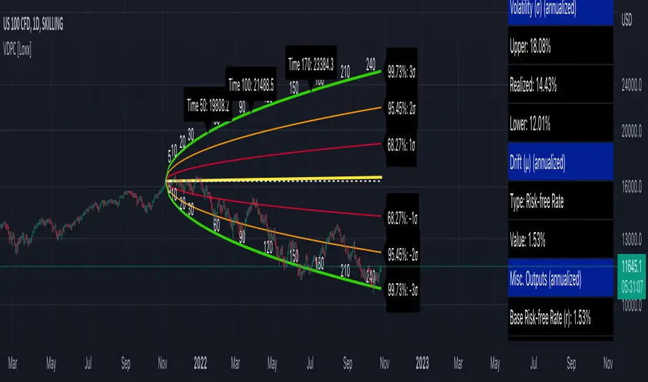
Confidence interval of volatility is calculated using an inverse CDF of a Chi-Squared Distribution. You change the volatility input used to create the probability cones from from realized volatility to upper or lower confidence levels of volatility to better visualize extremes of range. Generally, you'd stick with realized volatility.
Days per year should be 252 for everything but Cryptocurrency. These are days trader per year. Maximum future forecast bars is 365. Forecast bars are limited to the maximum of selected days per year.
Includes the ability to overlay option expiration dates by bars to see the range of prices for that date at that bar
You can select confidence % you wish for both the cone in general and the volatility. There are three levels for the cones, this will show on the three different levels up and down on the chart.
The table on the right displays important calculated values so you don't have to remember what they are or what settings you selected
All values are annualized no matter the timeframe.
Additional distributions and measures of volatility and drift will be added in future releases.
Skrip jemputan sahaja
Hanya pengguna yang diberikan kebenaran oleh penulis mempunyai akses kepada skrip ini dan ini selalunya memerlukan pembayaran. Anda boleh menambahkan skrip kepada kegemaran anda tetapi anda hanya boleh menggunakannya selepas meminta kebenaran dan mendapatkannya daripada penulis — ketarhui lebih lanjut di sini. Untuk lebih butiran, ikuti arahan penulis di bawah atau hubungi loxx secara terus.
TradingView tidak menyarankan pembayaran untuk atau menggunakan skrip kecuali anda benar-benar mempercayai penulisnya dan memahami bagaimana ia berfungsi. Anda juga boleh mendapatkan alternatif sumber terbuka lain yang percuma dalam skrip komuniti kami.
Arahan penulis
Amaran: sila baca panduan kami untuk skrip jemputan sahaja sebelum memohon akses.
VIP Membership Info: patreon.com/algxtrading/membership
Penafian
Skrip jemputan sahaja
Hanya pengguna yang diberikan kebenaran oleh penulis mempunyai akses kepada skrip ini dan ini selalunya memerlukan pembayaran. Anda boleh menambahkan skrip kepada kegemaran anda tetapi anda hanya boleh menggunakannya selepas meminta kebenaran dan mendapatkannya daripada penulis — ketarhui lebih lanjut di sini. Untuk lebih butiran, ikuti arahan penulis di bawah atau hubungi loxx secara terus.
TradingView tidak menyarankan pembayaran untuk atau menggunakan skrip kecuali anda benar-benar mempercayai penulisnya dan memahami bagaimana ia berfungsi. Anda juga boleh mendapatkan alternatif sumber terbuka lain yang percuma dalam skrip komuniti kami.
Arahan penulis
Amaran: sila baca panduan kami untuk skrip jemputan sahaja sebelum memohon akses.
VIP Membership Info: patreon.com/algxtrading/membership