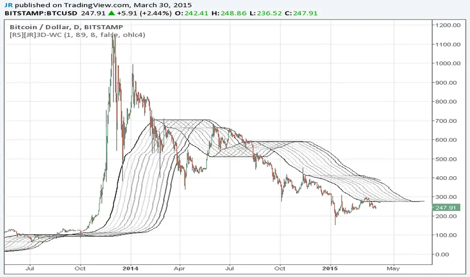
Wave Channel 3D — Petunjuk oleh QuantitativeExhaustion

wave parallelchannel 3d fibonacci multiplier offset support supportandresistance movingaverage

Wave Channel 3D
Built by Ricardo idea from JR & Aloakdutt from indieTrades Jan. 2010

This indicator is very easy to build. We utilize Moving Averages with a set multiplier and an offset. Specially we try to use Fibonacci sequence series numbers (1, 2, 3, 5, 8, 13, 21, 34, 55, 89, 144...) as time space and multiplier (default 89, 8). Also included is Donchian Channel to locate strong trends and possible future support - resistance.

Examples of support/resistance on chart.

Dominant Price Trends

Future Support Resistance

Comparing Fibonacci Series Time Space - Multiplier

When Comparing make note of confluence support/resistance showing up with Fibonacci Series
Example uses DC

When Comparing make note of confluence support/resistance showing up with Fibonacci Series
Example without DC / Smooth MA

Skrip sumber terbuka

Dalam semangat TradingView yang sebenar, penulis skrip ini telah menerbitkannya dengan menggunakan sumber terbuka supaya pedagang-pedagang dapat memahami dan mengesahkannya. Sorakan kepada penulis! Anda dapat menggunakannya secara percuma tetapi penggunaan semula kod ini dalam penerbitan adalah dikawalselia oleh Peraturan Dalaman. Anda boleh menyukainya untuk menggunakannya pada carta.

Penafian

Maklumat dan penerbitan adalah tidak dimaksudkan untuk menjadi, dan tidak membentuk, nasihat untuk kewangan, pelaburan, perdagangan dan jenis-jenis lain atau cadangan yang dibekalkan atau disahkan oleh TradingView. Baca dengan lebih lanjut di Terma Penggunaan.

Ingin menggunakan skrip ini pada carta?

study(title="3D-Wave Channel", shorttitle="3D-WC", overlay=true)
timespace = input(1)
smooth = input(89)
offsetMultiplier=input(8)
useDonchianAverage = input(false)
src = input(ohlc4)
ma = useDonchianAverage ? avg(highest(smooth),lowest(smooth)) : ema(src, smooth)
plot(ma[0], color=black, offset=offsetMultiplier*01)
plot(ma[timespace*01], color=silver, offset=offsetMultiplier*02)
plot(ma[timespace*02], color=silver, offset=offsetMultiplier*03)
plot(ma[timespace*03], color=gray, offset=offsetMultiplier*04)
plot(ma[timespace*04], color=gray, offset=offsetMultiplier*05)
plot(ma[timespace*05], color=gray, offset=offsetMultiplier*06)
plot(ma[timespace*06], color=silver, offset=offsetMultiplier*07)
plot(ma[timespace*07], color=silver, offset=offsetMultiplier*08)
plot(ma[timespace*08], color=gray, offset=offsetMultiplier*09)
plot(ma[timespace*09], color=gray, offset=offsetMultiplier*10)
plot(ma[timespace*10], color=black, offset=offsetMultiplier*11)

max_ma()=>max(ma[timespace*10],max(ma[timespace*9],max(ma[timespace*8],max(ma[timespace*7],max(ma[timespace*6],max(ma[timespace*5],max(ma[timespace*4],max(ma[timespace*3],max(ma[timespace*2],max(ma[timespace*1], ma))))))))))
min_ma()=>min(ma[timespace*10],min(ma[timespace*9],min(ma[timespace*8],min(ma[timespace*7],min(ma[timespace*6],min(ma[timespace*5],min(ma[timespace*4],min(ma[timespace*3],min(ma[timespace*2],min(ma[timespace*1], ma))))))))))

top = highest(max_ma(), smooth)
bot = lowest(min_ma(), smooth)

plot(top, color=black, offset=offsetMultiplier)
plot(bot, color=black, offset=offsetMultiplier)