VX Levels and Ranch Ranges with SPY/SPX price converterThis is a indicator for all Vexly subscribers to plot the following:
1. Plot SPY/SPX levels on your ES chart. Or QQQ levels on your NQ chart
2. VX levels obtained from vx_levels command. SPY on ES chart and QQQ on NQ chart
3. Ranch Range levels from the discord channel for ES and NQ chart.
You can enable/disable any of them at your discretion.
Educational

Z-Score & StatsThis is an advanced indicator that measures price deviation from its mean using statistical z-scores, combined with multiple analytical features for trading signals.
Core Functionality-
Z-Score Calculation Engine:
The indicator uses a custom standardization function that calculates how many standard deviations the current price is from its rolling mean. Unlike simple moving averages, this provides a normalized view of price extremes. The calculation maintains a sliding window of data points, efficiently updating mean and variance values as new data arrives while removing old data points. This approach handles missing values gracefully and uses sample variance (rather than population variance) for more accurate statistical measurements.
Statistical Zones & Visual Framework:
The indicator creates a visual representation of statistical probability zones:
±1 Standard Deviation: Encompasses about 68% of normal price behavior (green zone)
±2 Standard Deviations: Covers approximately 95% of price movements (orange zone)
±3 Standard Deviations: Represents 99.7% probability range (red zone)
±3.5 and ±4 Thresholds: Extreme outlier levels that trigger special alerts
The z-score line changes color dynamically based on which zone it occupies, making it easy to identify the current market extremity at a glance.
Advanced Features:
Volume Contraction Analysis
The script monitors volume patterns to identify periods of reduced trading activity. It compares current volume against a moving average and flags when volume drops below a specified threshold (default 70%). Volume contraction often precedes significant price moves and is factored into the optimal entry detection system.
Momentum-Based Direction Model:
Rather than just showing current z-score levels, the indicator projects where the z-score is likely to move based on recent momentum. It calculates the rate of change in the z-score and extrapolates forward for a specified number of bars. This creates a directional arrow that indicates whether conditions are bullish (negative z-score with upward momentum) or bearish (positive z-score with downward momentum).
Divergence Detection System:
The script automatically identifies four types of divergences between price action and z-score behavior :-
Regular Bullish Divergence: Price makes lower lows while z-score makes higher lows, suggesting weakening downward pressure
Regular Bearish Divergence: Price makes higher highs while z-score makes lower highs, indicating exhaustion in the uptrend
Hidden Bullish Divergence: Price makes higher lows while z-score makes lower lows, confirming trend continuation in an uptrend
Hidden Bearish Divergence: Price makes lower highs while z-score makes higher highs, confirming downtrend continuation
The system uses pivot detection with configurable lookback periods and distance requirements, then draws connecting lines and labels directly on the chart when divergences occur.
Yearly Statistics Tracking:
The indicator maintains historical records of maximum z-score deviations over yearly periods (configurable bar count). This provides context by showing whether current extremes are unusual compared to typical annual ranges. The average yearly maximum helps traders understand if the current market is exhibiting normal volatility or exceptional conditions.
Mean Reversion Probability:
Based on the current z-score magnitude, the indicator calculates and displays the statistical probability that price will revert toward the mean. Higher absolute z-scores indicate stronger mean reversion probabilities, ranging from 38% at ±0.5 standard deviations to 99.7% at ±3 standard deviations.
Comprehensive Statistics Table:
A customizable on-chart table displays real-time statistics including:
Current z-score value with directional indicator
Predicted z-score based on momentum
Current year's maximum absolute z-score
Historical average yearly maximum
Mean reversion probability percentage
Zone status classification (Normal, Moderate, High, Extreme)
Directional bias (Bullish, Bearish, Neutral)
Active divergence status
Volume contraction status with ratio
Optimal setup detection (combining extreme z-scores with volume contraction)
Optimal Entry Setup Detection:
The most sophisticated feature identifies high-probability trading setups by combining multiple factors. An "Optimal Long" signal triggers when z-score reaches -3.5 or below AND volume is contracted. An "Optimal Short" signal appears when z-score exceeds +3.5 AND volume is contracted. This combination suggests extreme price deviation occurring on low volume, often preceding strong reversals.
Alert System:
The script includes a unified alert mechanism that triggers when z-score crosses specific thresholds:
Crossing above/below ±3.5 standard deviations (extreme levels)
Crossing above/below ±4 standard deviations (critical levels)
Alerts fire once per bar with confirmation (previous bar must be on opposite side of threshold) to avoid false signals.
Practical Application:
This indicator is designed for mean reversion traders who seek statistically significant price extremes. The combination of z-score measurement, volume analysis, momentum projection, and divergence detection creates a multi-layered confirmation system. Traders can use extreme z-scores as potential reversal zones, while the direction model and divergence signals help time entries more precisely. The volume contraction filter adds an additional layer of confluence, identifying moments when reduced participation may precede explosive moves back toward the mean.
Chart Attached: NSE GMR Airports, EoD 12/12/25
DISCLAIMER: This information is provided for educational purposes only and should not be considered financial, investment, or trading advice.Happy Trading

VX-Time Quadrant Overlay (Quarterly Cycles) by Ikaru-s-The Time Quadrant Overlay is a purely time-based visualization tool designed to structure market time into repeating quarterly cycles across multiple timeframes.
It does not generate trade signals, entries, or bias.
Its sole purpose is to provide time context, so price action can be interpreted within a clear cyclical framework.
What this indicator does
The indicator divides time into four repeating quarters (Q1–Q4) and displays them simultaneously across different time horizons, such as:
Weekly
Daily (6-hour quarters)
90-minute cycles
Micro cycles (within 90-minute structure)
Each row represents a different time cycle, allowing traders to see time alignment, transitions, and overlaps at a glance.
Quarter Structure
Each cycle follows the same repeating sequence:
Q1 – Early phase
Q2 – Expansion / “True Open” phase
Q3 – Continuation
Q4 – Late phase / Transition
The quarters are visualized using color-coded boxes, making it easy to see:
where the market currently is in time
when a new quarter begins
when multiple cycles align or diverge
Quarter Start Marker
An optional Quarter Start Marker (vertical dashed line) can be enabled to highlight the start of a selected quarter (default: Q2).
This is intended as a time reference, not a signal:
useful for planning
useful for contextualizing reactions to levels
useful for session and cycle awareness
How to use it (practical)
This tool is best used to:
provide time structure to existing analysis
plan around upcoming time transitions
contextualize reactions to levels or areas
understand where price is acting within a cycle
It works well alongside:
discretionary price action
session-based trading
futures and index markets
any methodology that respects time as a variable
Customization
The indicator is fully customizable:
Enable / disable individual cycles
Adjust box transparency and history depth
Toggle labels and pane labels
Enable / disable quarter start markers
Select which quarter to highlight
This allows the tool to remain clean on higher timeframes and detailed on lower ones.
Important Notes
This is a visual framework, not a strategy.
No claims of predictive power are made.
Time structure does not replace risk management or execution logic.
The indicator is designed to adapt across markets, but interpretation remains discretionary.
Final Thoughts
Time is often treated as secondary to price.
This tool exists to make time visible, structured, and easy to work with — nothing more, nothing less.

FVG pointsFVGs ( fair value gaps) are imbalances that indicate displacement and are useful for reversal strategies that require displacement after a liquidity sweep
This indicator shows the size of the gap in points/dollars which can help determine momentum and strength in reversals, as does a failure or inversion (iFVG) of these gap if they fail to act as support or resistance to price. As stops are often placed on the other side of a fair value gap from entry, the indicator helps give traders an idea of stop loss size for calculating position size.
Fvg gaps below a certain points size can be considered to be weaker, larger gaps show stronger momentum. The indicator allows a minimum point size to be set so that FVGs below this minimum value will be shown without a points value.
Points value is also shown for inverted FVGs (iFVGs) by a change in colour and length of box.
By default, multiple gaps are combined together and the point value of the gap is shown, this can be toggled off in the settings to show the values of the individual gaps.
Settings:
Lookback - how many candles to look for FVGs and iFVGs
Change length of the FVG box
Change settings to decide the minimum size of gap to label
colours of boxes and labels
Option to show individual gaps or combined gaps

Liquidity Buy SignalLiquidity Buy Signal is an indicator designed to detect BUY entries based on liquidity (swing lows) combined with a bullish reversal candle pattern. It automatically marks recent swing-low zones/levels, tracks the transition from solid → dashed when a level gets broken, and then confirms a signal when price sweeps/cuts the correct level and a bullish candle pattern appears.
OANDA:EURUSD
BUY signal (green triangle) triggers when:
A bullish reversal candle pattern (based on a set of rules) is detected, and
The Liquidity chain conditions are satisfied using the most recent swing lows:
Price crosses the level with the lower wick, or
The level is within the lower 30% range of the previous candle (n-1), and
The level does not pass through the bodies of older candles (filtered by lookback).
Key settings:
Pivot Lookback: controls swing-low detection sensitivity.
Swing Area: Wick Extremity / Full Range for zone definition.
Filter lookback older bodies: filters out levels that intersect older candle bodies (skips n-2).
Style: toggle Swing Low display + zone/line colors.
Alerts:
Includes a built-in alertcondition for BUY signals (useful for notifications/webhooks).
This indicator is especially well-suited for identifying potential bottoms in a downtrend.
Note: This tool provides trading signals and should be combined with context (trend/HTF/volume/risk management) before entering trades. Not financial advice.

FxNeel SessionAll types of ICT session you can draw here. Like Asia, London, NY, New Close, CBDR, Asia Kill zone and also Silverbullet Time zone.

TWS- RSI+Divergence With Stochestic+Div. v21.0 By AshishThis indicator is for RSI & RSI Divergence. Also you can activate Stochastic (modified level) with divergence.
This is totally new concept. you can try it.

Volatility Targeting: Single Asset [BackQuant]Volatility Targeting: Single Asset
An educational example that demonstrates how volatility targeting can scale exposure up or down on one symbol, then applies a simple EMA cross for long or short direction and a higher timeframe style regime filter to gate risk. It builds a synthetic equity curve and compares it to buy and hold and a benchmark.
Important disclaimer
This script is a concept and education example only . It is not a complete trading system and it is not meant for live execution. It does not model many real world constraints, and its equity curve is only a simplified simulation. If you want to trade any idea like this, you need a proper strategy() implementation, realistic execution assumptions, and robust backtesting with out of sample validation.
Single asset vs the full portfolio concept
This indicator is the single asset, long short version of the broader volatility targeted momentum portfolio concept. The original multi asset concept and full portfolio implementation is here:
That portfolio script is about allocating across multiple assets with a portfolio view. This script is intentionally simpler and focuses on one symbol so you can clearly see how volatility targeting behaves, how the scaling interacts with trend direction, and what an equity curve comparison looks like.
What this indicator is trying to demonstrate
Volatility targeting is a risk scaling framework. The core idea is simple:
If realized volatility is low relative to a target, you can scale position size up so the strategy behaves like it has a stable risk budget.
If realized volatility is high relative to a target, you scale down to avoid getting blown around by the market.
Instead of always being 1x long or 1x short, exposure becomes dynamic. This is often used in risk parity style systems, trend following overlays, and volatility controlled products.
This script combines that risk scaling with a simple trend direction model:
Fast and slow EMA cross determines whether the strategy is long or short.
A second, longer EMA cross acts as a regime filter that decides whether the system is ACTIVE or effectively in CASH.
An equity curve is built from the scaled returns so you can visualize how the framework behaves across regimes.
How the logic works step by step
1) Returns and simple momentum
The script uses log returns for the base return stream:
ret = log(price / price )
It also computes a simple momentum value:
mom = price / price - 1
In this version, momentum is mainly informational since the directional signal is the EMA cross. The lookback input is shared with volatility estimation to keep the concept compact.
2) Realized volatility estimation
Realized volatility is estimated as the standard deviation of returns over the lookback window, then annualized:
vol = stdev(ret, lookback) * sqrt(tradingdays)
The Trading Days/Year input controls annualization:
252 is typical for traditional markets.
365 is typical for crypto since it trades daily.
3) Volatility targeting multiplier
Once realized vol is estimated, the script computes a scaling factor that tries to push realized volatility toward the target:
volMult = targetVol / vol
This is then clamped into a reasonable range:
Minimum 0.1 so exposure never goes to zero just because vol spikes.
Maximum 5.0 so exposure is not allowed to lever infinitely during ultra low volatility periods.
This clamp is one of the most important “sanity rails” in any volatility targeted system. Without it, very low volatility regimes can create unrealistic leverage.
4) Scaled return stream
The per bar return used for the equity curve is the raw return multiplied by the volatility multiplier:
sr = ret * volMult
Think of this as the return you would have earned if you scaled exposure to match the volatility budget.
5) Long short direction via EMA cross
Direction is determined by a fast and slow EMA cross on price:
If fast EMA is above slow EMA, direction is long.
If fast EMA is below slow EMA, direction is short.
This produces dir as either +1 or -1. The scaled return stream is then signed by direction:
avgRet = dir * sr
So the strategy return is volatility targeted and directionally flipped depending on trend.
6) Regime filter: ACTIVE vs CASH
A second EMA pair acts as a top level regime filter:
If fast regime EMA is above slow regime EMA, the system is ACTIVE.
If fast regime EMA is below slow regime EMA, the system is considered CASH, meaning it does not compound equity.
This is designed to reduce participation in long bear phases or low quality environments, depending on how you set the regime lengths. By default it is a classic 50 and 200 EMA cross structure.
Important detail, the script applies regime_filter when compounding equity, meaning it uses the prior bar regime state to avoid ambiguous same bar updates.
7) Equity curve construction
The script builds a synthetic equity curve starting from Initial Capital after Start Date . Each bar:
If regime was ACTIVE on the previous bar, equity compounds by (1 + netRet).
If regime was CASH, equity stays flat.
Fees are modeled very simply as a per bar penalty on returns:
netRet = avgRet - (fee_rate * avgRet)
This is not realistic execution modeling, it is just a simple turnover penalty knob to show how friction can reduce compounded performance. Real backtesting should model trade based costs, spreads, funding, and slippage.
Benchmark and buy and hold comparison
The script pulls a benchmark symbol via request.security and builds a buy and hold equity curve starting from the same date and initial capital. The buy and hold curve is based on benchmark price appreciation, not the strategy’s asset price, so you can compare:
Strategy equity on the chart symbol.
Buy and hold equity for the selected benchmark instrument.
By default the benchmark is TVC:SPX, but you can set it to anything, for crypto you might set it to BTC, or a sector index, or a dominance proxy depending on your study.
What it plots
If enabled, the indicator plots:
Strategy Equity as a line, colored by recent direction of equity change, using Positive Equity Color and Negative Equity Color .
Buy and Hold Equity for the chosen benchmark as a line.
Optional labels that tag each curve on the right side of the chart.
This makes it easy to visually see when volatility targeting and regime gating change the shape of the equity curve relative to a simple passive hold.
Metrics table explained
If Show Metrics Table is enabled, a table is built and populated with common performance statistics based on the simulated daily returns of the strategy equity curve after the start date. These include:
Net Profit (%) total return relative to initial capital.
Max DD (%) maximum drawdown computed from equity peaks, stored over time.
Win Rate percent of positive return bars.
Annual Mean Returns (% p/y) mean daily return annualized.
Annual Stdev Returns (% p/y) volatility of daily returns annualized.
Variance of annualized returns.
Sortino Ratio annualized return divided by downside deviation, using negative return stdev.
Sharpe Ratio risk adjusted return using the risk free rate input.
Omega Ratio positive return sum divided by negative return sum.
Gain to Pain total return sum divided by absolute loss sum.
CAGR (% p/y) compounded annual growth rate based on time since start date.
Portfolio Alpha (% p/y) alpha versus benchmark using beta and the benchmark mean.
Portfolio Beta covariance of strategy returns with benchmark returns divided by benchmark variance.
Skewness of Returns actually the script computes a conditional value based on the lower 5 percent tail of returns, so it behaves more like a simple CVaR style tail loss estimate than classic skewness.
Important note, these are calculated from the synthetic equity stream in an indicator context. They are useful for concept exploration, but they are not a substitute for professional backtesting where trade timing, fills, funding, and leverage constraints are accurately represented.
How to interpret the system conceptually
Vol targeting effect
When volatility rises, volMult falls, so the strategy de risks and the equity curve typically becomes smoother. When volatility compresses, volMult rises, so the system takes more exposure and tries to maintain a stable risk budget.
This is why volatility targeting is often used as a “risk equalizer”, it can reduce the “biggest drawdowns happen only because vol expanded” problem, at the cost of potentially under participating in explosive upside if volatility rises during a trend.
Long short directional effect
Because direction is an EMA cross:
In strong trends, the direction stays stable and the scaled return stream compounds in that trend direction.
In choppy ranges, the EMA cross can flip and create whipsaws, which is where fees and regime filtering matter most.
Regime filter effect
The 50 and 200 style filter tries to:
Keep the system active in sustained up regimes.
Reduce exposure during long down regimes or extended weakness.
It will always be late at turning points, by design. It is a slow filter meant to reduce deep participation, not to catch bottoms.
Common applications
This script is mainly for understanding and research, but conceptually, volatility targeting overlays are used for:
Risk budgeting normalize risk so your exposure is not accidentally huge in high vol regimes.
System comparison see how a simple trend model behaves with and without vol scaling.
Parameter exploration test how target volatility, lookback length, and regime lengths change the shape of equity and drawdowns.
Framework building as a reference blueprint before implementing a proper strategy() version with trade based execution logic.
Tuning guidance
Lookback lower values react faster to vol shifts but can create unstable scaling, higher values smooth scaling but react slower to regime changes.
Target volatility higher targets increase exposure and drawdown potential, lower targets reduce exposure and usually lower drawdowns, but can under perform in strong trends.
Signal EMAs tighter EMAs increase trade frequency, wider EMAs reduce churn but react slower.
Regime EMAs slower regime filters reduce false toggles but will miss early trend transitions.
Fees if you crank this up you will see how sensitive higher turnover parameter sets are to friction.
Final note
This is a compact educational demonstration of a volatility targeted, long short single asset framework with a regime gate and a synthetic equity curve. If you want a production ready implementation, the correct next step is to convert this concept into a strategy() script, add realistic execution and cost modeling, test across multiple timeframes and market regimes, and validate out of sample before making any decision based on the results.

Sideways Zone Breakout 📘 Sideways Zone Breakout – Indicator Description
Sideways Zone Breakout is a visual market-structure indicator designed to identify low-volatility consolidation zones and highlight potential breakout opportunities when price exits these zones.
This indicator focuses on detecting periods where price trades within a tight range, often referred to as sideways or consolidation phases, and visually marks these zones directly on the chart for clarity.
🔍 Core Concept
Markets often spend time moving sideways before making a directional move.
This indicator aims to:
Detect price compression
Visually highlight the sideways zone
Signal when price breaks above or below the zone boundaries
Instead of predicting direction, it simply reacts to range expansion after consolidation.
⚙️ How the Indicator Works
1️⃣ Sideways Zone Detection
The indicator looks back over a user-defined number of candles
It calculates the highest high and lowest low within that window
If the total price range remains within a defined percentage of the current price, the market is considered sideways
This helps filter out trending and highly volatile conditions.
2️⃣ Visual Zone Representation
When a sideways condition is detected:
A clear price zone is drawn between the recent high and low
The zone is displayed using a soft gradient fill for better visibility
Outer borders are added to enhance zone clarity without cluttering the chart
This makes consolidation areas easy to spot at a glance.
3️⃣ Breakout Identification
Once a sideways zone is active:
A bullish breakout is marked when price closes above the upper boundary
A bearish breakout is marked when price closes below the lower boundary
Directional arrows and labels are plotted directly on the chart to indicate these events.
📊 Visual Elements Included
Sideways consolidation zones with gradient fill
Upper and lower zone boundaries
Buy and Sell arrows on breakout
Optional text labels for clear interpretation
All visuals are designed to remain lightweight and readable on any chart theme.
🔧 User Inputs
Sideways Lookback (candles): Controls how many past candles are used to define the range
Max Range % (tightness): Determines how tight the range must be to qualify as sideways
Adjusting these inputs allows users to adapt the indicator to different instruments and timeframes.
📈 Usage Guidelines
Can be applied to any market or timeframe
Works well as a context or confirmation tool
Best used alongside volume, trend, or risk management tools
Signals should be validated with proper trade planning
⚠️ Disclaimer
This indicator is provided as open-source for educational and analytical purposes only.
It does not generate trade recommendations or guarantee outcomes.
Market conditions vary, and users are responsible for their own trading decisions.

S&R + EMA ToolkitThis script is a market-structure toolkit that combines several indicators into a single view to help understand where price is, where it may react, and what the current trend context is.
EMAs (12, 26, 50, 200)
Help define short-, medium-, and long-term trend context and momentum alignment.
Support & Resistance Channels
Help identify key price zones where the market has historically reacted (areas of acceptance, rejection, and consolidation).
Supertrend
Helps confirm directional bias and trend persistence.
Oversold / Overbought RSI Zones (external source)
Help identify market conditions rather than timing entries.
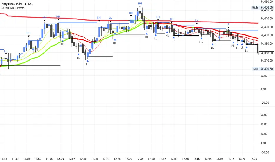
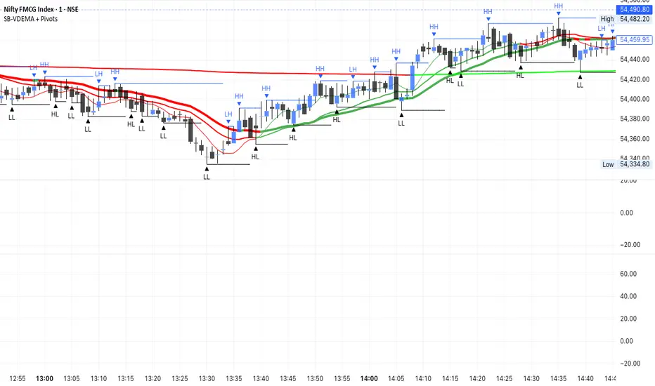
SB-VDEMA + PivotsBest use - Intraday Scalping ( 1 Mt, 3 Mts, 5 Mts )
Uses Volatility weighted DEMA for smoother and reliable signals.
One can use dynamic colour coding of VWDEMA for entering call or puts. VWAP and Henkin ashi Supertrend is also there but, i think VWDEMA is quite enogh for decision making.
SB - Ultimate Clean Trend Pro Uses dynamic Moving colour coding for spotting chage of bias. Use set up with keeping VWAP in reference.
Auto Trend [theUltimator5]The Auto Trend indicator was designed to be a unique pattern detection indicator without the use of standard pivot point logic or high/low lines. It is a study in pattern detection by using iterative best-fit logic.
The indicator automatically identifies and draws trend channels by analyzing price action across configurable lookback periods. It finds optimal high and low trendlines that contain price movement, with a middle line marking the trend's center.
Key Features:
Automatic Pattern Detection - Intelligently searches for the best lookback period where price stays within the channel boundaries
Dual Pattern Modes - Choose between Short (20-66 bars) for quick patterns or Long (50-500 bars) for extended trends. Note - the long pattern is fully configurable and can be set anywhere up to 5000 bars.
Smart Caching - Optimized performance that only recalculates when necessary
Customizable Starting Point - Click directly on the chart to set where the trend channel begins
Flexible Lookback Range - Set minimum and maximum lookback periods to match your trading style
Visual Debugging - Optional label displays the active lookback period and violation count
How It Works:
The indicator divides the lookback period into thirds, finds the highest and lowest closes in the first and last thirds, then draws trendlines connecting these points. It can automatically search through different lookback periods to find the one with the fewest price violations (closes outside the channel).
Settings:
Use Auto Lookback - Enable automatic optimal lookback detection
Pattern Length - Short (faster, 1-bar increments) or Long (broader, 5-bar increments)
Min/Max Lookback - Define the search range for the Long pattern
Manual Lookback - Override auto-detection with a fixed period
Custom Colors - Personalize the high, low, and middle line colors
Starting Point - Select where the trend analysis begins
Use Cases:
Identify dominant trend channels across different timeframes
Spot potential support and resistance levels
Determine trend strength and consistency
Time entries and exits based on channel position
The indicator supports up to 5000 bars of historical data for comprehensive trend analysis.

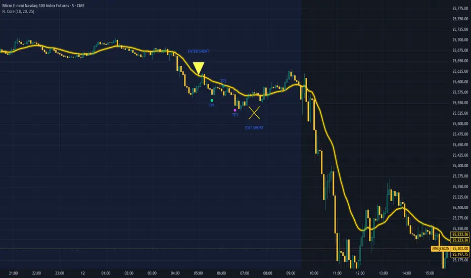
FL Core Signals Only FL Core shows only what matters: where to enter, where to exit, and where prof
No indicator noise — just confirmed decision points on a clean chart.
Designed for traders who value structure, patience, and clarity.
What FL Core Does
FL Core marks:
ENTER LONG
ENTER SHORT
AND
EXIT SHORT
TP1 / TP2 / TP3 profit targets
All signals are generated using a fixed, non-repainting ruleset and are confirmed only after candle close.
How It Trades (High Level)
Identifies momentum shifts using internal trend logic
Requires a full candle confirmation before signaling entries
Holds trades until momentum breaks, then signals exit
Tracks profit targets automatically in points
No guessing. No anticipation. No repainting.
Session Rules
FL Core is hard-wired to operate only between 4:00 AM and 4:00 PM (exchange time).
Signals outside of this window are intentionally ignored to avoid low-liquidity and overnight conditions.
Chart Design Philosophy
This version intentionally hides all underlying indicators and displays only:
Clean entry markers
Clean exit markers
Profit plate
A single gold Exit Rail that visually guides trade management
The focus stays on execution and decision-making, not indicator interpretation.
Profit Targets
Default profit targets are:
TP1: 25 points
TP2: 40 points
TP3: 60 p
Targets can be adjusted by the user.
Note: Default profit targets are optimized for NQ/MNQ, which was the primary instrument used during testing.
Traders using ES/MES should reduce target distances to better match volatility.
Important Notes
FL Core is an indicator, not an automated trading system
Stop-loss placement is handled manually according to your trading plan
Signals are designed to encourage discipline and patience, not over-trading
Marker placement (above/below bar) is intentional and should not be changed
Who This Is For
✔ Beginner traders
✔ Traders overwhelmed by indicators
✔ Traders who want clear structure and rules
✔ Traders focused on execution discipline
Who This Is NOT For
✘ Traders looking for fully automated execution
✘ Traders who want constant signals
✘ Traders who ignore risk management
Final Thought
FL Core does not try to predict the market.
It helps you wait for confirmation, execute cleanly, and manage trades with structure.
If you want fewer decisions, clearer trades, and a calmer trading experience — this is where you start.
Session Levels (Daily & Weekly Targets)This indicator provides market structure and contextual reference only. It does not generate trade signals, entries, or trading advice.
Plots rolling previous daily and weekly highs/lows as potential target levels. Levels automatically remove once touched (including wicks). Default visibility is NY session with optional toggles for London and Asia. Designed for intraday structure, confluence, and target identification.

Fibonacci Fibonacci automatic drawing - Last 144 barFibonacci automatic drawing:
It automatically plots Fibonacci based on the last 144 bars.
According to the drawing rules, it calculates itself from bottom to top and from top to bottom.
This will answer the most challenging questions about drawing the right thing.
If 144 bar is not reached, it draws using manual input.
This will be a useful and practical perspective.
This is for those who want to see the most valuable Fibonacci values on a chart.

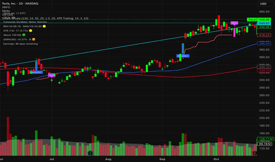
Smart WhaleOverview The Smart Whale Breakout System is a pure momentum strategy designed for Swing Traders who want to capture high-probability breakouts while managing risk with a mechanical trailing stop.
Unlike indicators that try to guess "bottoms," this system follows the "Smart Money" approach: buying strength when institutional volume enters, and riding the trend until the momentum breaks.
How it Works
1. The Entry (The Hunter) The system identifies a valid BREAKOUT signal only when four specific conditions align:
Trend Filter: Price must be above the 150 SMA. We only trade with the long-term trend.
Momentum: RSI > 50. Ensuring bulls are in control.
Volume Spike (Whale Activity): Current volume must be significantly higher than the average (Default: 1.5x). This filters out weak retail moves.
Price Action: A bullish candle closing higher than it opened.
2. The Exit (The Manager) Once in a trade, the system activates a dynamic Trailing Stop line. You never have to guess when to sell. You can choose between two exit logic modes in the settings:
ATR Trailing (Default): Adapts to volatility. The stop moves up based on a multiple of the Average True Range (ATR). Great for volatile stocks (e.g., TSLA, NVDA).
Percent Trailing: A fixed percentage drop from the highest high. (e.g., "Sell if price drops 10% from peak").
3. The Context (Optional Filter)
Squeeze Filter: Includes a built-in Bollinger/Keltner squeeze detection. If enabled in settings, the system will only signal a buy if the price recently broke out of a consolidation (squeeze). Default is OFF to catch all momentum moves.
Key Features
NO Repainting: Signals are confirmed at candle close.
Visual Risk Management: A Red Trailing Stop line clearly shows where your invalidation point is.
Fully Customizable: Adjust the Volume multiplier, ATR sensitivity, or Percentage drop to fit your asset class (Crypto/Stocks/Forex).
Clean Visuals: Only colors the Breakout and Sell candles to keep your chart clean.
Settings Guide
Trend SMA Length: Define the long-term trend baseline (Default: 150).
Volume Spike (xAvg): How much volume is needed to trigger a buy? (1.5 = 150% of average).
Exit Method: Choose between "ATR Trailing" or "Percent Trailing".
ATR Multiplier: Tighter stop (2.0) vs Looser stop (3.0).
Require Squeeze?: Check this to filter for breakouts that only happen after a consolidation period.
Disclaimer This tool is for educational purposes only. Always use proper risk management.
BIGG CHIEFF RWB MASTER v2.0 (Indicator) [v1.0]Here is a **clean, professional TradingView indicator description** you can paste directly into the script description. It explains the *logic and philosophy* without exposing proprietary specifics, while still sounding robust and credible.
---
## 📊 Indicator Overview
This indicator is a **rule-based EMA crossover strategy built on price action, opening range structure, directional bias, and momentum confirmation**.
It is designed for intraday trading during the New York session and adapts to both time-based and tick-based charts.
The system focuses on **clarity, patience, and consistency**, filtering out low-quality conditions while aligning trades with higher-probability market structure.
---
## 🧭 Core Concepts
### Opening Range Structure
* The strategy uses the **first 15 minutes of the New York session** to define an Opening Range.
* This range establishes **key intraday structure**, including:
* High
* Low
* Midpoint
* The Opening Range remains visible for the entire session and resets each day.
* Trades are framed around **breaks, retests, and rejections** of this structure.
---
## 📈 Trend, Bias & Momentum
### Directional Bias
Bias is determined by:
* **EMA stacking order**
* **Price location relative to the Opening Range**
* Optional **higher-timeframe trend alignment**
Once bias is confirmed:
* Trades are only taken **in the direction of that bias**
* Opposing trades are locked out until structure meaningfully changes
This prevents overtrading and reduces whipsaws in choppy conditions.
---
### Higher-Timeframe Alignment (Optional)
A higher-timeframe trend filter can be enabled to:
* Keep trades aligned with the broader market direction
* Improve win rate during trending sessions
* Reduce countertrend entries
---
## ⚡ Volatility & Time Filters
To avoid low-quality trades, the system includes:
* **Volatility filtering** to prevent entries during compressed or dead markets
* **Session time windows** to focus on the most liquid trading hours
* Optional **no-trade time blocks** for news or known high-risk periods
---
## 💧 Liquidity Awareness
The indicator accounts for **key liquidity zones**, such as:
* Prior session highs and lows
* Overnight and premarket extremes
Trades are filtered to ensure there is **sufficient room for reward** before running into nearby liquidity, helping avoid premature exits.
---
## ✅ Entry Logic (Primary Mode)
Trades are based on **structure first, confirmation second**:
* Breakouts must be confirmed by **candle closes**, not wicks
* Entries occur on **retracements and rejection candles**, not chase candles
* Priority is given to cleaner retests closer to structure
* Optional controls allow limiting trades to **first-touch setups only**
This encourages patience and avoids emotional entries.
---
## 🛑 Risk Management & Trade Management
The system is built around **R-multiple consistency**, not fixed targets.
* Stops are volatility-based
* Multiple profit targets can be enabled
* Optional partial profits and trailing stop logic are included
* Trailing behavior can follow momentum or structure once price moves favorably
Everything is designed to **protect capital first and scale winners second**.
---
## 🧠 Philosophy
This indicator is not designed to predict the market.
It is designed to **react intelligently** to what price is already confirming.
It prioritizes:
* Structure over indicators
* Bias over impulse
* Confirmation over hope
* Risk management over win rate
Best results come from disciplined execution, patience, and respecting the filters.

FVG + Inversion + MidlineThis is a rough version. Still in works.
Off Mode - Shows bullish and bearish FVGS
Only Mode - Only shows inverted FVGs in white (those above price are usually resistance zones and below tend to be support with the more recent and higher timeframe ones being most relevant)
Blended - Shows Both
You can adjust the amount of zones to be shown to modify the lookback period.
You can also adjust the price range by a standard deviation of 100% to only cover a specific price range.
Rest of the features are still being cleaned or irrelevant for the most part.

Star V12⭐ Star Engine — Multi-Component, Multi-Timeframe Trade Execution System
The Star Engine is a stateful trade execution and analytics system designed to transform indicator confluence into structured, measurable trade runs. Rather than producing isolated buy/sell signals, the engine decomposes market behavior into pressure, confirmation, event grouping, and trade lifecycle management. Each component plays a specific role, and no single component is sufficient on its own. Below is a detailed breakdown of each subsystem and why it exists.
💣 Bomb Engine — Directional Pressure Measurement
The Bomb Engine is responsible for identifying directional pressure in the market. It evaluates whether price action exhibits sustained momentum in one direction, independent of whether that direction is immediately tradable.
What Bomb Uses
Bomb aggregates momentum- and trend-oriented inputs such as MACD-based momentum direction, momentum persistence and continuation logic, directional bias filters, and impulse strength evaluation. All inputs are evaluated across multiple timeframes, with each timeframe contributing independently.
How Bomb Works
Each timeframe produces a directional contribution (bullish, bearish, or neutral). Contributions are aggregated into a net Bomb total. The total is mapped into discrete tone buckets (blue, green, red, black, etc.). Higher totals indicate stronger directional dominance.
What Bomb Tells You
Bomb answers one question: Is there directional pressure building or persisting? It does not determine entry timing, exhaustion, or trade quality. Bomb is context, not execution. This allows Bomb to be early without being responsible for precision.
✨ Golden Engine — Structural Confirmation & Regime Filtering
The Golden Engine evaluates whether the directional pressure detected by Bomb is structurally supported. Golden exists to prevent entries during momentum exhaustion, conflicting timeframe regimes, and counter-structure moves.
What Golden Uses
Golden relies on a different indicator stack than Bomb, focused on confirmation and balance, including RSI regime classification (not simple overbought/oversold), momentum agreement vs divergence, trend-following vs counter-trend positioning, overextension detection, and compression and rotational behavior. Each timeframe is evaluated independently using the same logic.
The Role of RSI in Golden
RSI in Golden is used to identify regimes, not signals. It answers questions such as: Is momentum expanding or decaying? Is the move early, mid-structure, or extended? Do multiple timeframes share compatible RSI states? If RSI regimes conflict across timeframes, Golden will not confirm. This is one of the main mechanisms that makes Golden selective.
Momentum & Alignment Logic
Golden evaluates whether momentum supports continuation, is fragmenting, is diverging from price, or is contradicting higher-timeframe structure. If lower-timeframe impulses are not supported by higher-timeframe structure, Golden suppresses confirmation — even if Bomb remains strong.
What Golden Guarantees
Golden does not guarantee profitable trades. Golden guarantees that the detected directional pressure is not internally contradictory across RSI regimes, momentum behavior, and timeframe structure. This replaces vague terms like “clean” with explicit structural conditions.
🔗 Multi-Timeframe Aggregation (MTF)
Both Bomb and Golden operate on a multi-timeframe voting system. Lower timeframes capture early impulses, higher timeframes enforce structural context, each timeframe votes independently, conflicts weaken totals, and alignment strengthens totals. This creates temporal confluence, not just price-based confluence.
⭐ Star Events — Qualified Market Impulses
A Star (⭐) is created only when Bomb is active, Golden is active, both agree on direction, and all gating rules pass (thresholds, time filters, modes). A Star represents a qualified impulse, not a trade. Stars are atomic events used by the execution layer.
⏱ Star Clusters — Trade Run State
The Star Cluster groups Stars into runs. The first Star starts a cluster, anchor price, bar, and time are recorded, each additional Star increments the cluster count, and all Stars belong to the same run until exit. This prevents duplicate entries, signal spam, and overtrading in volatile conditions.
⛔ Reset Gap Logic — Temporal Control
To prevent rapid re-entry, a minimum time gap is required to start a new run. Stars occurring too close together are merged. Reset does not terminate active runs. This enforces time-based discipline, not indicator-based guessing.
1➡️ Entry Logic — Confirmation-Based Execution
The engine never enters on the first Star. Instead, the user defines 🔢 N (Entry Star Index). Entry occurs only on the Nth Star, and that bar is marked 1➡️🔢N. This ensures entries occur after persistence, not detection. At ENTRY, Best = 0.00 and Worst = 0.00. Statistics measure real trade performance, not early signal noise.
📊 STAT Engine — Live Trade Measurement
Once entry is active, the STAT engine tracks ⏱ run progression, 🏅 maximum favorable excursion, and 📉 maximum adverse excursion. Mechanics: uses highs and lows, not closes; updates every bar; entry bar resets stats; historical bars marked 🎨. This creates an objective performance envelope for every trade.
🛑 Exit Engine — Deterministic Outcomes
Trades are exited using explicit rules: 🏅 WIN → profit threshold reached, 📉 LOSE → risk threshold breached, ⏱ QUIT → structural or safety exit.
Safety Exits
🐢 Idle Stop — no Stars for N bars.
🧯 Freeze Failsafe — STAT inactivity.
QUIT is a controlled termination, not failure. Each exit is recorded with a short cause tag.
🧾 Trade Memory & Journaling
Every trade produces immutable records. Entry: time, price, side, confirmation index. Exit: time, price, PnL, result, cause. These records power tables, alerts, JSON output, and external automation.
📊 Time-Block Performance (NY Clock)
Performance is grouped by real time, not bar count. Rolling NY blocks (e.g. 3 hours). Independent statistics per block. Live trades persist across block boundaries. This enables session-based analysis.
🔔 Alerts & Automation
Alerts are state-based: Entry confirmed → Long / Short alert. Trade closed → Exit alert. Optional JSON output allows integration with bots, journals, and dashboards.
Summary
The Star Engine is a component-based trade execution system, where Bomb measures pressure, Golden validates structure, Stars qualify impulses, clusters define runs, entry is delayed by confirmation, stats measure reality, exits are deterministic, and results are time-aware. It is not designed to “predict the market”, but to control how trades are formed, managed, and evaluated.

Straight Regression Line + Normalized Slope (Adaptive Length)Find the regression line of available candles.
It will print the slope and the normalized slope

VX Levels and Ranch Ranges with Price ConverterThis is a indicator for all Vexly subscribers to plot the following:
1. Plot SPY/SPX levels on your ES chart. Or QQQ levels on your NQ chart
2. VX levels obtained from vx_levels command. SPY on ES chart and QQQ on NQ chart
3. Ranch Range levels from the discord channel for ES and NQ chart.
You can enable/disable any of them at your discretion.
GVWAP_Core (CalendarSpan + EventSpike)GVWAP Core Indicator
General Description (Public)
GVWAP (Generalized Volume-Weighted Average Price) is an advanced anchoring and averaging framework designed to reveal market structure rather than predict price. Unlike traditional VWAP, GVWAP is not limited to volume weighting or session-based anchoring. It can operate on any input series (price, indicators, transforms) and supports multiple weighting schemes, decay behavior, and structural reset logic.
At its core, GVWAP answers a simple question: “Where is the statistically relevant center of activity since the last meaningful structural event?”
The indicator continuously updates a weighted average of the input series, gradually forgetting older data using exponential decay. The anchor point can reset on calendar boundaries (day, week, month, etc.) or on statistically significant events such as abnormal volume spikes. Robust dispersion bands based on mean absolute deviation (MAD) surround the average, providing context for trend, rotation, and compression regimes.
GVWAP is not a trading signal by itself. It is best used as a structural reference layer or as an intermediate transform feeding other indicators, strategies, or regime filters.
Mathematical Description (Quantitative)
Let x_t be an arbitrary input series and w_t a selectable weight function. GVWAP is defined as a normalized exponentially decayed weighted estimator:
GVWAP_t = N_t / D_t
with recursive updates:
N_t = (1 − α)·N_{t−1} + α·w_t·x_t
D_t = (1 − α)·D_{t−1} + α·w_t
where α = 1 − 2^(−1/H) and H is the decay half-life in bars.
Weights may be defined as:
• w_t = V_t (volume)
• w_t = 1 (equal weight)
• w_t = 1 / ATR_t (volatility-normalized)
• w_t = f(n_t) (time-weighted, where n_t is bars since reset)
The estimator resets when a structural condition R_t is satisfied, at which point:
N_t = w_t·x_t, D_t = w_t
For event-based anchoring, volume surprise is computed using a Student‑t–compressed z‑score:
z_t = (V_t − μ_V) / σ_V
tZ_t = z_t / sqrt(1 + z_t² / ν)
A reset occurs when tZ_t exceeds a threshold τ.
Dispersion is measured via a decayed Mean Absolute Deviation:
MAD_t = (Σ λ^{t−i} w_i |x_i − GVWAP_t|) / (Σ λ^{t−i} w_i)
Bands are defined as GVWAP_t ± k·MAD_t.
GVWAP therefore represents a bounded-memory, robust, non‑Gaussian estimator of the local conditional expectation of x_t under dynamic anchoring and weighting.