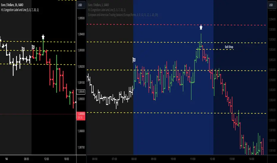
European and American Trading Sessions (Blue)The European and American trading sessions, in particular, are known for their volatility and volume, making them key periods for traders to watch.
This Pine Script indicator, "European and American Trading Sessions," helps traders visually distinguish these sessions directly on their charts by shading the background during active hours. We use this indicator in combination with the one that highlights the nighttime phases in white.
Here's a breakdown of how the indicator works:
Key Features of the Script:
Timezone Configuration:
The script allows users to select a timezone from a predefined list that includes UTC, London, Rome, New York, and Tokyo. This flexibility ensures that the session times are accurately displayed regardless of the server or local time of the user.
European Session Parameters:
Users can set the start and end times for the European session. By default, the session runs from 08:00 to 12:00, but the input options make it customizable down to the minute. The European session is highlighted with a light blue background (36% opacity) to avoid overwhelming the chart while still providing a clear visual cue.
American Session Parameters:
Similar to the European session, the American session can be customized. The default times are set from 12:01 to 20:59. This session is highlighted in a slightly darker blue (80% opacity), providing a distinct visual difference from the European session.
Session Timing Calculation:
The script calculates the start and end times for each session based on the selected timezone. It uses the timestamp() function to account for year, month, day, hour, and minute, ensuring that session timings are accurately applied to each day’s trading activity.
Background Highlighting:
Once the session times are defined, the script checks if the current chart time (time) falls within the European or American trading session. If the condition is true, the corresponding background color is applied, visually highlighting the active session directly on the chart. This feature makes it easy to identify when the European or American markets are in play.
Benefits for Traders:
Clear Session Visibility: The color-coded background makes it effortless for traders to identify when key trading sessions are active without needing to constantly check the clock.
Customizable to Your Needs:
With full control over the start and end times for both sessions, traders can adapt the indicator to fit their specific trading hours or preferences.
Timezone Flexibility:
No matter where you're trading from, the ability to set the timezone ensures that the sessions are displayed correctly according to your local time.
Explanation of the Code:
Timezone Selection:
Allows the user to select a timezone from predefined options such as Europe/Rome, America/New_York, etc. This timezone will be used to calculate session start and end times.
Session Timing Inputs:
The script takes user inputs for the start and end times of the European and American trading sessions. These inputs include the hour and minute for both sessions.
Colors:
The color of the European session is set to a blue shade with 36% opacity.
The American session is also colored blue but with a higher opacity of 80%.
Timestamp Calculation:
The timestamp() function converts the input hours and minutes into a time value, accounting for the selected timezone.
Session Conditions:
The script checks if the current time (time) falls within the European or American session. If true, it applies the respective background color for that session. This approach creates clear visual highlights on the chart, marking the active hours of the European and American trading sessions based on user inputs.
Cari dalam skrip untuk "跨境通12月4日地天板"
Sessions Full Markets [TradingFinder] Forex Stocks Index 7 Time🔵 Introduction
In global financial markets, particularly in FOREX and stocks, precise timing of trading sessions plays a crucial role in the success of traders. Each trading session—Asian, European, and American—has its own unique characteristics in terms of volatility and trading volume.
The Asian session (Tokyo), Sydney session, Shanghai session, European session (London and Frankfurt), and American session (New York AM and New York PM) are examples of these trading sessions, each of which opens and closes at specific times.
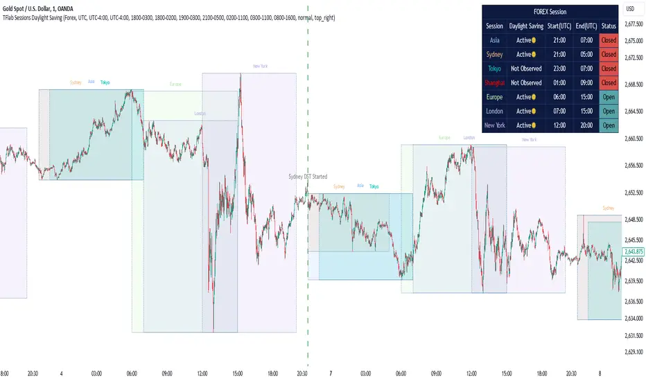
This session indicator also includes a Time Convertor, enabling users to view FOREX market hours based on GMT, UTC, EST, and local time. Another valuable feature of this indicator is the automatic detection of Daylight Saving Time (DST), which automatically applies time changes for the New York, London, and Sydney sessions.
🔵 How to Use
The indicator also displays session times based on the exact opening and closing times for each geographic region. Users can utilize this indicator to view trading hours either locally or in UTC time, and if needed, set their own custom trading times.
Additionally, the session information table includes the start and end times of each session and whether they are open or closed. This functionality helps traders make better trading decisions by using accurate and precise time data.
Key Features of the Session Indicator
The session indicator is a versatile and advanced tool that provides several unique features for traders.
Some of these features are :
• Automatic Daylight Saving Time (DST) Detection : This indicator dynamically detects Daylight Saving Time (DST) changes for various trading sessions, including New York, London, and Sydney, without requiring manual adjustments. This feature allows traders to manage their trades without worrying about time changes.
Below are the start and end dates for DST in the New York, London, and Sydney trading sessions :
1. New York :
Start of DST: Second Sunday of March, at 2:00 AM.
End of DST: First Sunday of November, at 2:00 AM
2. London :
Start of DST: Last Sunday of March, at 1:00 AM.
End of DST: Last Sunday of October, at 2:00 AM.
3. Sydney :
Start of DST: First Sunday of October, at 2:00 AM.
End of DST: First Sunday of April, at 3:00 AM.
• Session Display Based on Different Time Zones : The session indicator allows users to view trading times based on different time zones, such as UTC, the local time of each market, or the user’s local time. This feature is especially useful for traders operating in diverse geographic regions.
• Custom Trading Time Setup : Another notable feature of this indicator is the ability to set custom trading times. Traders can adjust their own trading times according to their personal strategies and benefit from this flexibility.
• Session Information Table : The session indicator provides a complete information table that includes the exact start and end times of each trading session and whether they are open or closed. This table helps users simultaneously and accurately monitor the status of all trading sessions and make better trading decisions.
🟣 Session Trading Hours Based on Market Mode and Time Zones
The session indicator provides precise information on the start and end times of trading sessions.
These times are adjusted based on different market modes (FOREX, stocks, and TFlab suggestions) and time zones (UTC and local time) :
🟣 (FOREX Session Time) Forex Market Mode
• Sessions in UTC (DST inactive) :
Sydney: 22:00 - 06:00
Tokyo: 23:00 - 07:00
Shanghai: 01:00 - 09:00
Asia: 22:00 - 07:00
Europe: 07:00 - 16:00
London: 08:00 - 16:00
New York: 13:00 - 21:00
• Sessions in UTC (DST active) :
Sydney: 21:00 - 05:00
Tokyo: 23:00 - 07:00
Shanghai: 01:00 - 09:00
Asia: 21:00 - 07:00
Europe: 06:00 - 15:00
London: 07:00 - 15:00
New York: 12:00 - 20:00
• Sessions in Local Time :
Sydney: 08:00 - 16:00
Tokyo: 08:00 - 16:00
Shanghai: 09:00 - 17:00
Asia: 22:00 - 07:00
Europe: 07:00 - 16:00
London: 08:00 - 16:00
New York: 08:00 - 16:00
🟣 Stock Market Trading Hours (Stock Market Mode)
• Sessions in UTC (DST inactive) :
Sydney: 00:00 - 06:00
Asia: 00:00 - 06:00
Europe: 07:00 - 16:30
London: 08:00 - 16:30
New York: 14:30 - 21:00
Tokyo: 00:00 - 06:00
Shanghai: 01:30 - 07:00
• Sessions in UTC (DST active) :
Sydney: 23:00 - 05:00
Asia: 23:00 - 06:00
Europe: 06:00 - 15:30
London: 07:00 - 15:30
New York: 13:30 - 20:00
Tokyo: 00:00 - 06:00
Shanghai: 01:30 - 07:00
• Sessions in Local Time:
Sydney: 10:00 - 16:00
Tokyo: 09:00 - 15:00
Shanghai: 09:30 - 15:00
Asia: 00:00 - 06:00
Europe: 07:00 - 16:30
London: 08:00 - 16:30
New York: 09:30 - 16:00
🟣 TFlab Suggestion Mode
• Sessions in UTC (DST inactive) :
Sydney: 23:00 - 05:00
Tokyo: 00:00 - 06:00
Shanghai: 01:00 - 09:00
Asia: 23:00 - 06:00
Europe: 07:00 - 16:00
London: 08:00 - 16:00
New York: 13:00 - 21:00
• Sessions in UTC (DST active) :
Sydney: 22:00 - 04:00
Tokyo: 00:00 - 06:00
Shanghai: 01:00 - 09:00
Asia: 22:00 - 06:00
Europe: 06:00 - 15:00
London: 07:00 - 15:00
New York: 12:00 - 20:00
• Sessions in Local Time :
Sydney: 09:00 - 16:00
Tokyo: 09:00 - 15:00
Shanghai: 09:00 - 17:00
Asia: 23:00 - 06:00
Europe: 07:00 - 16:00
London: 08:00 - 16:00
New York: 08:00 - 16:00
🔵 Setting
Using the session indicator is straightforward and practical. Users can add this indicator to their trading chart and take advantage of its features.
The usage steps are as follows :
Selecting Market Mode : The user can choose one of the three main modes.
Forex Market Mode: Displays the forex market trading hours.
oStock Market Mode: Displays the trading hours of stock exchanges.
Custom Mode: Allows the user to set trading hours based on their needs.
TFlab Suggestion Mode: Displays the higher volume hours of the forex market in Asia.
Setting the Time Zone : The indicator allows displaying sessions based on various time zones. The user can select one of the following options:
UTC (Coordinated Universal Time)
Local Time of the Session
User’s Local Time
Displaying Comprehensive Session Information : The session information table includes the opening and closing times of each session and whether they are open or closed. This table helps users monitor all sessions at a glance and precisely set the best time for entering and exiting trades.
🔵Conclusion
The session indicator is a highly efficient and essential tool for active traders in the FOREX and stock markets. With its unique features, such as automatic DST detection and the ability to display sessions based on different time zones, the session indicator helps traders to precisely and efficiently adjust their trading activities.
This indicator not only shows users the exact opening and closing times of sessions, but by providing a session status table, it helps traders identify the best times to enter and exit trades. Moreover, the ability to set custom trading times allows traders to easily personalize their trading schedules according to their strategies.
In conclusion, using the session indicator ensures that traders are continuously and accurately informed of time changes and the opening and closing hours of markets, eliminating the need for manual updates to align with DST changes. These features enable traders to optimize their trading strategies with greater confidence and up-to-date information, allowing them to capitalize on opportunities in the market.
ToS█ OVERVIEW
Contains methods for conversion to string of simple types int/float/bool/string/line/label/box .
- toS() - For bool/int/float works much the same as str.tostring() with some shorthand formatting options for int/float. For line/label/box displays their text and coordinates automatically formatting x coordinate as time or bar index.
- toShortString() - Converts a number to a short form using "k", "m", "bn" and "T" nominators. (e.g. `12,350` --> `12.4k`).
Supports some shorthand formatting options for int/float and time.
█ HOW TO USE
All toS() methods have the same parameters:
Parameters:
val (int) : A float to be converted to string
format (string) : Format string, which depends on the value type
nz (string) : (string) A string used to represent na (na values are substituted with this string).
For toS(bool/int/float) format parameter works in the same way as `str.format()` (i.e. you can use same format strings as with `str.format()` with `{0}` as a placeholder for the value)
Some shorthand "format" options available:
--- number ---
- "" => "{0}"
- "number" => "{0}"
- "0" => "{0, number, 0 }"
- "0.0" => "{0, number, 0.0 }"
- "0.00" => "{0, number, 0.00 }"
- "0.000" => "{0, number, 0.000 }"
- "0.0000" => "{0, number, 0.0000 }"
- "0.00000" => "{0, number, 0.00000 }"
- "0.000000" => "{0, number, 0.000000 }"
- "0.0000000" => "{0, number, 0.0000000}"
--- date ---
- "... ... " in any place is substituted with "{0, date, dd.MM.YY}"
- "date" => "{0, date, dd.MM.YY}"
- "date : time" => "{0, date, dd.MM.YY} : {0, time, HH.mm.ss}"
- "dd.MM" => "{0, date, dd:MM}"
- "dd" => "{0, date, dd}"
--- time ---
- "... ... " in any place is substituted with "{0, time, HH.mm.ss}"
- "time" => "{0, time, HH:mm:ss}"
- "HH:mm" => "{0, time, HH:mm}"
- "mm:ss" => "{0, time, mm:ss}"
- "date time" => "{0, date, dd.MM.YY\} {0, time, HH.mm.ss}"
- "date, time" => "{0, date, dd.MM.YY\}, {0, time, HH.mm.ss}"
- "date,time" => "{0, date, dd.MM.YY\},{0, time, HH.mm.ss}"
- "date\ntime" => "{0, date, dd.MM.YY\}\n{0, time, HH.mm.ss}"
For toS(line) :
format (string) : (string) (Optional) Use `x1` as placeholder for `x1` and so on. E.g. default format is `"(x1, y1) - (x2, y2)"`.
For toS(label) :
format (string) : (string) (Optional) Use `x1` as placeholder for `x`, `y1 - for `y` and `txt` for label's text. E.g. default format is `(x1, y1): "txt"` if ptint_text is true and `(x1, y1)` if false.
For toS(box) :
format (string) : (string) (Optional) Use `x1` as placeholder for `x`, `y1 - for `y` etc. E.g. default format is "(x1, y1) - (x2, y2)".
For toS(color) :
format (string) : (string) (Optional) Options are "HEX" (e.g. "#FFFFFF33") or "RGB" (e.g. "rgb(122,122,122,23)"). Default is "HEX".
█ LIST OF FUNCTIONS AND PARAMETERS
method toS(val, format, nz)
Formats the `int/float` in the same way as `str.format()` (i.e. you can use same format strings as with
`str.format()` with `{0}` arg) with some shorthand "format" options:
```
--- number ---
- "" => "{0}"
- "number" => "{0}"
- "0" => "{0, number, 0 }"
- "0.0" => "{0, number, 0.0 }"
- "0.00" => "{0, number, 0.00 }"
- "0.000" => "{0, number, 0.000 }"
- "0.0000" => "{0, number, 0.0000 }"
- "0.00000" => "{0, number, 0.00000 }"
- "0.000000" => "{0, number, 0.000000 }"
- "0.0000000" => "{0, number, 0.0000000}"
--- date ---
- "......" in angular brackets in any place is substituted with "{0, date, dd.MM.YY}"
- "date" => "{0, date, dd.MM.YY}"
- "date : time" => "{0, date, dd.MM.YY} : {0, time, HH.mm.ss}"
- "dd.MM" => "{0, date, dd:MM}"
- "dd" => "{0, date, dd}"
--- time ---
- "......" in angular brackets in any place is substituted with "{0, time, HH.mm.ss}"
- "time" => "{0, time, HH:mm:ss}"
- "HH:mm" => "{0, time, HH:mm}"
- "mm:ss" => "{0, time, mm:ss}"
- "date time" => "{0, date, dd.MM.YY\} {0, time, HH.mm.ss}"
- "date, time" => "{0, date, dd.MM.YY\}, {0, time, HH.mm.ss}"
- "date,time" => "{0, date, dd.MM.YY\},{0, time, HH.mm.ss}"
- "date\ntime" => "{0, date, dd.MM.YY\}\n{0, time, HH.mm.ss}"
```
Namespace types: series int, simple int, input int, const int
Parameters:
val (int) : A float to be converted to string
format (string) : Format string (e.g. "0.000" or "date : time" or "HH:mm")
nz (string) : (string) A string used to represent na (na values are substituted with this string).
method toS(val, format, nz)
Formats the `int/float` in the same way as `str.format()` (i.e. you can use same format strings as with
`str.format()` with `{0}` arg) with some shorthand "format" options:
```
--- number ---
- "" => "{0}"
- "number" => "{0}"
- "0" => "{0, number, 0 }"
- "0.0" => "{0, number, 0.0 }"
- "0.00" => "{0, number, 0.00 }"
- "0.000" => "{0, number, 0.000 }"
- "0.0000" => "{0, number, 0.0000 }"
- "0.00000" => "{0, number, 0.00000 }"
- "0.000000" => "{0, number, 0.000000 }"
- "0.0000000" => "{0, number, 0.0000000}"
--- date ---
- "......" in angular brackets in any place is substituted with "{0, date, dd.MM.YY}"
- "date" => "{0, date, dd.MM.YY}"
- "date : time" => "{0, date, dd.MM.YY} : {0, time, HH.mm.ss}"
- "dd.MM" => "{0, date, dd:MM}"
- "dd" => "{0, date, dd}"
--- time ---
- "......" in angular brackets in any place is substituted with "{0, time, HH.mm.ss}"
- "time" => "{0, time, HH:mm:ss}"
- "HH:mm" => "{0, time, HH:mm}"
- "mm:ss" => "{0, time, mm:ss}"
- "date time" => "{0, date, dd.MM.YY\} {0, time, HH.mm.ss}"
- "date, time" => "{0, date, dd.MM.YY\}, {0, time, HH.mm.ss}"
- "date,time" => "{0, date, dd.MM.YY\},{0, time, HH.mm.ss}"
- "date\ntime" => "{0, date, dd.MM.YY\}\n{0, time, HH.mm.ss}"
```
Namespace types: series float, simple float, input float, const float
Parameters:
val (float) : A float to be converted to string
format (string) : Format string (e.g. "0.000" or "date : time" or "HH:mm")
nz (string) : (string) A string used to represent na (na values are substituted with this string).
method toS(val, format, nz)
Formats `bool val` in the same way as `str.format()` (i.e. you can use same format strings as with
`str.format()` with `{0}` placeholder for the `val` argument).
Namespace types: series bool, simple bool, input bool, const bool
Parameters:
val (bool) : (bool) Value to be formatted
format (string)
nz (string) : (string) A string used to represent na (na values are substituted with this string).
method toS(val, format, nz)
Formats `string val` in the same way as `str.format()` (i.e. you can use same format strings as with
`str.format()` with `{0}` placeholder for the `val` argument).
Namespace types: series color, simple color, input color, const color
Parameters:
val (color)
format (string) : (string) "HEX" or "RGB"
nz (string) : (string) A string used to represent na (na values are substituted with this string).
method toS(val, format, nz)
Formats `string val` in the same way as `str.format()` (i.e. you can use same format strings as with
`str.format()` with `{0}` placeholder for the `val` argument).
Namespace types: series string, simple string, input string, const string
Parameters:
val (string)
format (string)
nz (string) : (string) A string used to represent na (na values are substituted with this string).
method toS(ln, format, nz)
Returns line's coordinates as a string (by default in "(x1, y1) - (x2, y2)" format, use `x1`, `y1`, `x2`,`y2` as placeholders in `format` string)). Automatically detects
whether the coordinates are in `xloc.bar_index` or `xloc.bar_time` and displays
accordingly (in _dd.MM.yy HH:mm:ss_ format)
Namespace types: series line
Parameters:
ln (line)
format (string) : (string) (Optional) Use `x1` as placeholder for `x1` and so on. E.g. default format is `"(x1, y1) - (x2, y2)"`.
nz (string) : (string) (Optional) If `val` is `na` and `nz` is not `na` the value of `nz` param is returned instead.
method toS(lbl, format, nz, print_text)
Returns label's coordinates and text as a string (by default in "(x, y): text = ...)" format; use `x1`, `y1`, `txt` as placeholders in `format` string))).
Automatically detects whether the coordinates are in `xloc.bar_index` or `xloc.bar_time` and displays.
accordingly (in _dd.MM.yy HH:mm:ss_ format)
Namespace types: series label
Parameters:
lbl (label)
format (string) : (string) (Optional) Use `x1` as placeholder for `x`, `y1 - for `y` and `txt` for label's text. E.g. default format is `(x1, y1): "txt"`.
nz (string) : (string) A string used to represent na (na values are substituted with this string).
print_text (bool)
method toS(bx, format, nz)
Returns box's coordinates as a string (by default in "(x1, y1) - (x2, y2)" format)
Namespace types: series box
Parameters:
bx (box)
format (string) : (string) (Optional) Use `x1` as placeholder for `x`, `y1 - for `y` etc. E.g. default format is "(x1, y1) - (x2, y2)".
nz (string) : (string) A string used to represent na (na values are substituted with this string).
method toShortString(this, decimals)
Converts number to a short form using "k", "m", "bn" and "T" nominators. (e.g. `12,350` --> `12.4k`).
@this (series float) Number to be converted to short format.
@decimals (series int) Optional argument. Decimal places to which number will be rounded. When no argument
is supplied, rounding is to the nearest integer.
Namespace types: series float, simple float, input float, const float
Parameters:
this (float)
decimals (int)

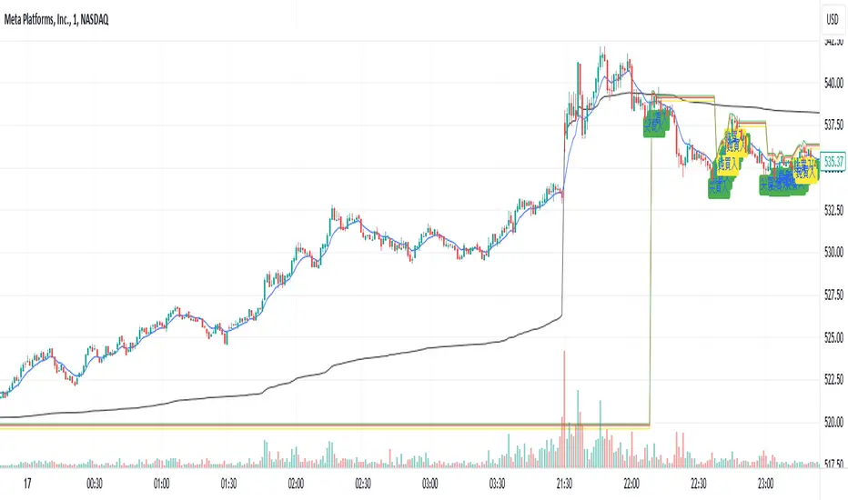
Backside Bubble ScalpingFrom LIHKG
Pine from Perplexity AI
以下是Backside Bubble Scalping策略的使用說明,旨在幫助交易者理解如何在美股交易中應用這一策略。
使用說明:Backside Bubble Scalping 策略
1. 前提條件
交易時間:此策略適用於香港時間晚上9:30 PM至12:00 AM。
圖表類型:使用1分鐘圖表進行交易。
2. 策略概述
Backside Bubble Scalping策略包含兩種主要的設置:尖backside和鈍backside。這些設置通常在10:00 PM至12:00 AM之間出現。
3. 指標設定
VWAP(粉紅色):成交量加權平均價格,用於識別市場趨勢。
9 EMA(綠色):9期指數移動平均線,用於捕捉短期價格變化。
4. 識別 Backside 設置
尖backside
特徵:
當市場趨勢為純紅色下跌,並形成尖尖的V形底部。
入場條件:
當價格突破9 EMA並經過小幅盤整後,進場做多。
鈍backside
特徵:
在混合顏色的趨勢中,形成鈍鈍的V形底部。
入場條件:
在盤整期間進場做多。
5. 止損和止盈設置
止損位置:
尖backside:設置在9 EMA上方的盤整範圍底部加上0.2。
鈍backside:設置在V底部的最低點加上0.2。
止盈位置:
尖backside:當價格跌破VWAP或出現一根K線沒有跟隨時出場。
鈍backside:當一根K線的三分之二身體向下突破9 EMA時出場。
6. 操作步驟
監控市場動態:在指定的交易時間內,觀察VWAP和9 EMA的變化。
識別入場信號:根據尖backside或鈍backside的條件進行判斷,確定何時進場。
設置止損和止盈:根據上述條件設置止損和止盈位,以管理風險。
執行交易:根據信號執行交易,並持續監控市場情況以調整策略。
7. 注意事項
避免在VWAP附近進行交易,以減少失敗風險。
如果出現影線(wick bar),建議不要進行交易,因為這可能表示該設置失敗。
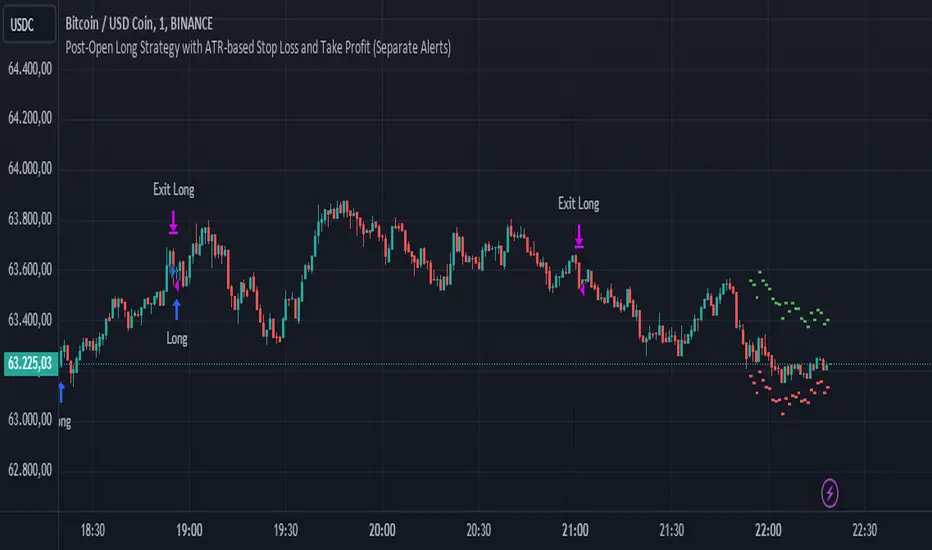
Post-Open Long Strategy with ATR-based Stop Loss and Take ProfitThe "Post-Open Long Strategy with ATR-Based Stop Loss and Take Profit" is designed to identify buying opportunities after the German and US markets open. It combines various technical indicators to filter entry signals, focusing on breakout moments following price lateralization periods.
Key Components and Their Interaction:
Bollinger Bands (BB):
Description: Uses BB with a 14-period length and standard deviation multiplier of 1.5, creating narrower bands for lower timeframes.
Role in the Strategy: Identifies low volatility phases (lateralization). The lateralization condition is met when the price is near the simple moving average of the BB, suggesting an imminent increase in volatility.
Exponential Moving Averages (EMA):
10-period EMA: Quickly detects short-term trend direction.
200-period EMA: Filters long-term trends, ensuring entries occur in a bullish market.
Interaction: Positions are entered only if the price is above both EMAs, indicating a consolidated positive trend.
Relative Strength Index (RSI):
Description: 7-period RSI with a threshold above 30.
Role in the Strategy: Confirms the market is not oversold, supporting the validity of the buy signal.
Average Directional Index (ADX):
Description: 7-period ADX with 7-period smoothing and a threshold above 10.
Role in the Strategy: Assesses trend strength. An ADX above 10 indicates sufficient momentum to justify entry.
Average True Range (ATR) for Dynamic Stop Loss and Take Profit:
Description: 14-period ATR with multipliers of 2.0 for Stop Loss and 4.0 for Take Profit.
Role in the Strategy: Adjusts exit levels based on current volatility, enhancing risk management.
Resistance Identification and Breakout:
Description: Analyzes the highs of the last 20 candles to identify resistance levels with at least two touches.
Role in the Strategy: A breakout above this level signals a potential continuation of the bullish trend.
Time Filters and Market Conditions:
Trading Hours: Operates only during the opening of the German market (8:00 - 12:00) and US market (15:30 - 19:00).
Panic Candle: The current candle must close negative, leveraging potential emotional reactions in the market.
Avoiding Entry During Pullbacks:
Description: Checks that the two previous candles are not both bearish.
Role in the Strategy: Avoids entering during a potential pullback, improving trade success probability.
Post-Open Long Strategy with ATR-Based Stop Loss and Take Profit
The "Post-Open Long Strategy with ATR-Based Stop Loss and Take Profit" is designed to identify buying opportunities after the German and US markets open. It combines various technical indicators to filter entry signals, focusing on breakout moments following price lateralization periods.
Key Components and Their Interaction:
Bollinger Bands (BB):
Description: Uses BB with a 14-period length and standard deviation multiplier of 1.5, creating narrower bands for lower timeframes.
Role in the Strategy: Identifies low volatility phases (lateralization). The lateralization condition is met when the price is near the simple moving average of the BB, suggesting an imminent increase in volatility.
Exponential Moving Averages (EMA):
10-period EMA: Quickly detects short-term trend direction.
200-period EMA: Filters long-term trends, ensuring entries occur in a bullish market.
Interaction: Positions are entered only if the price is above both EMAs, indicating a consolidated positive trend.
Relative Strength Index (RSI):
Description: 7-period RSI with a threshold above 30.
Role in the Strategy: Confirms the market is not oversold, supporting the validity of the buy signal.
Average Directional Index (ADX):
Description: 7-period ADX with 7-period smoothing and a threshold above 10.
Role in the Strategy: Assesses trend strength. An ADX above 10 indicates sufficient momentum to justify entry.
Average True Range (ATR) for Dynamic Stop Loss and Take Profit:
Description: 14-period ATR with multipliers of 2.0 for Stop Loss and 4.0 for Take Profit.
Role in the Strategy: Adjusts exit levels based on current volatility, enhancing risk management.
Resistance Identification and Breakout:
Description: Analyzes the highs of the last 20 candles to identify resistance levels with at least two touches.
Role in the Strategy: A breakout above this level signals a potential continuation of the bullish trend.
Time Filters and Market Conditions:
Trading Hours: Operates only during the opening of the German market (8:00 - 12:00) and US market (15:30 - 19:00).
Panic Candle: The current candle must close negative, leveraging potential emotional reactions in the market.
Avoiding Entry During Pullbacks:
Description: Checks that the two previous candles are not both bearish.
Role in the Strategy: Avoids entering during a potential pullback, improving trade success probability.
Entry and Exit Conditions:
Long Entry:
The price breaks above the identified resistance.
The market is in a lateralization phase with low volatility.
The price is above the 10 and 200-period EMAs.
RSI is above 30, and ADX is above 10.
No short-term downtrend is detected.
The last two candles are not both bearish.
The current candle is a "panic candle" (negative close).
Order Execution: The order is executed at the close of the candle that meets all conditions.
Exit from Position:
Dynamic Stop Loss: Set at 2 times the ATR below the entry price.
Dynamic Take Profit: Set at 4 times the ATR above the entry price.
The position is automatically closed upon reaching the Stop Loss or Take Profit.
How to Use the Strategy:
Application on Volatile Instruments:
Ideal for financial instruments that show significant volatility during the target market opening hours, such as indices or major forex pairs.
Recommended Timeframes:
Intraday timeframes, such as 5 or 15 minutes, to capture significant post-open moves.
Parameter Customization:
The default parameters are optimized but can be adjusted based on individual preferences and the instrument analyzed.
Backtesting and Optimization:
Backtesting is recommended to evaluate performance and make adjustments if necessary.
Risk Management:
Ensure position sizing respects risk management rules, avoiding risking more than 1-2% of capital per trade.
Originality and Benefits of the Strategy:
Unique Combination of Indicators: Integrates various technical metrics to filter signals, reducing false positives.
Volatility Adaptability: The use of ATR for Stop Loss and Take Profit allows the strategy to adapt to real-time market conditions.
Focus on Post-Lateralization Breakout: Aims to capitalize on significant moves following consolidation periods, often associated with strong directional trends.
Important Notes:
Commissions and Slippage: Include commissions and slippage in settings for more realistic simulations.
Capital Size: Use a realistic trading capital for the average user.
Number of Trades: Ensure backtesting covers a sufficient number of trades to validate the strategy (ideally more than 100 trades).
Warning: Past results do not guarantee future performance. The strategy should be used as part of a comprehensive trading approach.
With this strategy, traders can identify and exploit specific market opportunities supported by a robust set of technical indicators and filters, potentially enhancing their trading decisions during key times of the day.
Essa's Indicator 2.0Essa's Indicator V2: Beginner's Guide
This custom TradingView indicator has been designed to help you identify key trading opportunities based on session highs/lows, volatility, and moving averages. Below is a breakdown of the main features:
1. Exponential Moving Averages (EMAs)
Fast EMA (Blue Line): Tracks the short-term market trend (default: 9-period EMA).
Slow EMA (Red Line): Tracks the longer-term market trend (default: 21-period EMA).
You can turn on/off the EMAs using the "Show EMAs" option in the settings.
EMAs help smooth out price action and give a clearer picture of trends. A crossover of the fast EMA above the slow EMA can signal an upward trend, while the reverse may indicate a downward trend.
2. Session Highs and Lows
The indicator tracks price highs and lows for three major trading sessions:
London Session (Red): Highlighted in red. Active between 08:00 and 17:00 (LDN timezone) or 03:00 and 12:00 (NY timezone).
New York Session (Blue): Highlighted in blue. Active between 12:00 and 21:00 (LDN timezone) or 07:00 and 16:00 (NY timezone).
Asia Session (Yellow): Highlighted in yellow. Active between 22:00 and 08:00 (LDN timezone) or 18:00 and 03:00 (NY timezone).
Highs and lows for each session are plotted on the chart as lines. Breakouts from these levels can signal important trading opportunities:
London High/Low: Red lines.
New York High/Low: Blue lines.
Asia High/Low: Yellow lines.
The background color also changes depending on the active session:
London: Light red background.
New York: Light blue background.
Asia: Light yellow background.
3. Breakout Alerts
You can set alerts when the price breaks above or below session highs/lows:
Break Above London High: Alert triggered when the price crosses the London session high.
Break Below London Low: Alert triggered when the price falls below the London session low.
Similar alerts exist for the New York and Asia sessions as well.
4. Volatility-Adjusted EMA
The EMAs in this indicator are adjusted based on volatility (ATR - Average True Range). This allows the EMAs to respond to market conditions more dynamically, giving you more accurate trend readings in volatile markets.
5. ZigZag Feature (Optional)
You can enable the ZigZag feature to help visualize the price action's highs and lows:
ZigZag Lines: Highlight major peaks and troughs in price movements, helping you spot trends more easily.
This is helpful for identifying reversals or trend continuations.
6. Fractal Markers
This indicator uses fractals to mark potential turning points in the market:
Green Triangles (Above the Price): Indicate up fractals (potential reversal points where the price could move upwards).
Red Triangles (Below the Price): Indicate down fractals (potential reversal points where the price could move downwards).
Fractals can be a helpful confirmation tool when identifying entry and exit points.
7. Custom Timezone Options
You can choose between London (LDN) and New York (NY) timezones in the settings to adapt the session times to your trading location. This ensures the session high/low markers are displayed correctly for your trading region.
By default, the New York (NY) timezone is enabled for FXCM charts in the UK.
For BTC charts, you will need to switch to the appropriate time zone manually.
Thanks
Essa

Volume Wave Trend ConfirmationUtility of the Indicator
The core utility of this indicator lies in its ability to utilize volume, a less frequently exploited metric in MACD analysis, providing several strategic advantages:
Trend Confirmation: By focusing on volume, the indicator confirms whether movements in price are backed by significant trading activity. A rising MACD line above the signal line, paired with increasing volume, can confirm the strength of an uptrend. Conversely, if the histogram turns negative while the MACD line falls below the signal line during a price drop, it confirms a robust downtrend.
Early Warning Signals: Changes in the histogram and divergences between the MACD and Signal lines can serve as early warnings of potential reversals or slowdowns in market momentum. For instance, a shrinking histogram in an uptrend might suggest that the upward movement is losing steam.
Market Sentiment: The integration of volume into the MACD framework allows the indicator to provide insights into underlying market sentiment. Higher volumes during price movements indicate stronger conviction among traders, making the trend more reliable.
Indicator Functionality
The "Volume Wave Trend Confirmation" indicator is built on the Moving Average Convergence Divergence (MACD) framework, but with a unique twist: it uses the smoothed moving averages (SMA) of trading volumes instead of price. The indicator calculates two specific SMAs of the volume — a shorter 33-period SMA and a longer 100-period SMA — and computes their difference. This difference is then used as the input for the MACD calculation, with typical parameters set at 12, 26, and a signal line of 9.
MACD Line (Blue): Represents the main line, calculated as the difference between the 12-period and 26-period exponential moving averages (EMA) of the volume difference.
Signal Line (Orange): A 9-period EMA of the MACD line, acting as a trigger for buy or sell signals.
Histogram (Blue/Purple): Measures the distance between the MACD line and the Signal line, colored blue when positive (above the Signal line) and purple when negative (below the Signal line).

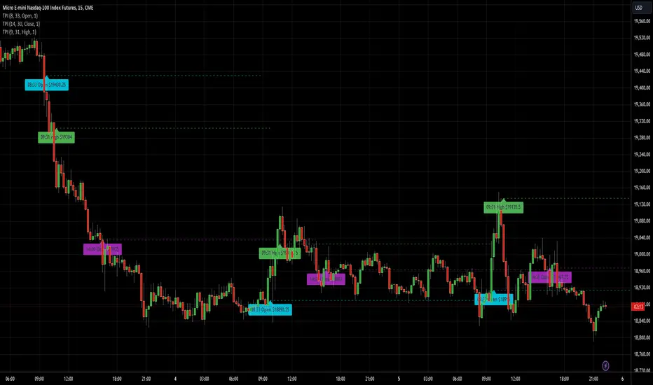
AnyTimeAndPrice
This indicator allows users to input a specific start time and display the price of a lower timeframe on a higher timeframe chart. It offers customization options for:
- Display name
- Label color
- Line extension
By adding multiple instances of the AnyTimeframeTimeAndPrice indicator, each customized for different times and prices, you can create a powerful and flexible tool for analyzing market data. Here's a potential setup:
1. Instance 1:
- Time: 08:23
- Price: Open
- Display Name: "8:23 Open"
- Label Color: Green
2. Instance 2:
- Time: 12:47
- Price: High
- Display Name: "12:47 High"
- Label Color: Red
3. Instance 3:
- Time: 15:19
- Price: Low
- Display Name: "3:19 Low"
- Label Color: Blue
4. Instance 4:
- Time: 16:53
- Price: Close
- Display Name: "4:53 Close"
- Label Color: Yellow
By having multiple instances, you can:
- Track different times and prices on the same chart
- Customize the display names, label colors, and line extensions for each instance
- Easily compare and analyze the relationships between different times and prices
This setup can be particularly useful for:
- Identifying key levels and support/resistance areas
- Analyzing market trends and patterns
- Making more informed trading decisions
Inputs:
1. AnyStartHour: Integer input for the start hour (default: 09, range: 0-23)
2. AnyStartMinute: Integer input for the start minute (default: 30, range: 0-59)
3. Sourcename: String input for the display name (default: "Open", options: "Open", "Close", "High", "Low")
4. Src_col: Color input for the label color (default: aqua)
5. linetimeExtMulti: Integer input for the line time extension (default: 1, range: 1-5)
Calculations:
1. AnyinputStartTime: Timestamp for the input start time
2. inputhour and inputminute: Hour and minute components of the input start time
3. formattedAnyTime: Formatted string for the input start time (HH:mm)
4. currenttime: Current timestamp
5. currenthour and currentminute: Hour and minute components of the current time
6. formattedTime: Formatted string for the current time (HH:mm)
7. onTime and okTime: Boolean flags for checking if the current time matches the input start time or is within the session
8. firstbartime: Timestamp for the first bar of the session
9. dailyminutesfromSource: Calculation for the daily minutes from the source
10. anyminSrcArray: Request security lower timeframe array for the source
11. ltf (lower timeframe): Integer variable for tracking the lower timeframe
12. Sourcevalue: Float variable for storing the source value
13. linetimeExt: Integer variable for line extension (calculated from linetimeExtMulti)
Logic:
1. Check if the current time matches the input start time or is within the session
2. If true, plot a line and label with the source value and formatted time
3. If not, check if the current time is within the daily session and plot a line and label accordingly
Notes:
- The script uses request.security_lower_tf to request data from a lower timeframe
- The script uses line.new and label.new to plot lines and labels on the chart
- The script uses str.format_time to format timestamps as strings (HH:mm)
- The script uses xloc.bar_time to position lines and labels at the bar time
This script allows users to input a specific start time and display the price of a lower timeframe on a higher timeframe chart, with options for customizing the display name, label color, and line extension.
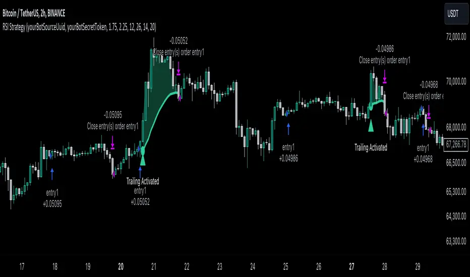
RSI Trend Following StrategyOverview
The RSI Trend Following Strategy utilizes Relative Strength Index (RSI) to enter the trade for the potential trend continuation. It uses Stochastic indicator to check is the price is not in overbought territory and the MACD to measure the current price momentum. Moreover, it uses the 200-period EMA to filter the counter trend trades with the higher probability. The strategy opens only long trades.
Unique Features
Dynamic stop-loss system: Instead of fixed stop-loss level strategy utilizes average true range (ATR) multiplied by user given number subtracted from the position entry price as a dynamic stop loss level.
Configurable Trading Periods: Users can tailor the strategy to specific market windows, adapting to different market conditions.
Two layers trade filtering system: Strategy utilizes MACD and Stochastic indicators measure the current momentum and overbought condition and use 200-period EMA to filter trades against major trend.
Trailing take profit level: After reaching the trailing profit activation level script activates the trailing of long trade using EMA. More information in methodology.
Wide opportunities for strategy optimization: Flexible strategy settings allows users to optimize the strategy entries and exits for chosen trading pair and time frame.
Methodology
The strategy opens long trade when the following price met the conditions:
RSI is above 50 level.
MACD line shall be above the signal line
Both lines of Stochastic shall be not higher than 80 (overbought territory)
Candle’s low shall be above the 200 period EMA
When long trade is executed, strategy set the stop-loss level at the price ATR multiplied by user-given value below the entry price. This level is recalculated on every next candle close, adjusting to the current market volatility.
At the same time strategy set up the trailing stop validation level. When the price crosses the level equals entry price plus ATR multiplied by user-given value script starts to trail the price with trailing EMA(by default = 20 period). If price closes below EMA long trade is closed. When the trailing starts, script prints the label “Trailing Activated”.
Strategy settings
In the inputs window user can setup the following strategy settings:
ATR Stop Loss (by default = 1.75)
ATR Trailing Profit Activation Level (by default = 2.25)
MACD Fast Length (by default = 12, period of averaging fast MACD line)
MACD Fast Length (by default = 26, period of averaging slow MACD line)
MACD Signal Smoothing (by default = 9, period of smoothing MACD signal line)
Oscillator MA Type (by default = EMA, available options: SMA, EMA)
Signal Line MA Type (by default = EMA, available options: SMA, EMA)
RSI Length (by default = 14, period for RSI calculation)
Trailing EMA Length (by default = 20, period for EMA, which shall be broken close the trade after trailing profit activation)
Justification of Methodology
This trading strategy is designed to leverage a combination of technical indicators—Relative Strength Index (RSI), Moving Average Convergence Divergence (MACD), Stochastic Oscillator, and the 200-period Exponential Moving Average (EMA)—to determine optimal entry points for long trades. Additionally, the strategy uses the Average True Range (ATR) for dynamic risk management to adapt to varying market conditions. Let's look in details for which purpose each indicator is used for and why it is used in this combination.
Relative Strength Index (RSI) is a momentum indicator used in technical analysis to measure the speed and change of price movements in a financial market. It helps traders identify whether an asset is potentially overbought (overvalued) or oversold (undervalued), which can indicate a potential reversal or continuation of the current trend.
How RSI Works? RSI tracks the strength of recent price changes. It compares the average gains and losses over a specific period (usually 14 periods) to assess the momentum of an asset. Average gain is the average of all positive price changes over the chosen period. It reflects how much the price has typically increased during upward movements. Average loss is the average of all negative price changes over the same period. It reflects how much the price has typically decreased during downward movements.
RSI calculates these average gains and losses and compares them to create a value between 0 and 100. If the RSI value is above 70, the asset is generally considered overbought, meaning it might be due for a price correction or reversal downward. Conversely, if the RSI value is below 30, the asset is considered oversold, suggesting it could be poised for an upward reversal or recovery. RSI is a useful tool for traders to determine market conditions and make informed decisions about entering or exiting trades based on the perceived strength or weakness of an asset's price movements.
This strategy uses RSI as a short-term trend approximation. If RSI crosses over 50 it means that there is a high probability of short-term trend change from downtrend to uptrend. Therefore RSI above 50 is our first trend filter to look for a long position.
The MACD (Moving Average Convergence Divergence) is a popular momentum and trend-following indicator used in technical analysis. It helps traders identify changes in the strength, direction, momentum, and duration of a trend in an asset's price.
The MACD consists of three components:
MACD Line: This is the difference between a short-term Exponential Moving Average (EMA) and a long-term EMA, typically calculated as: MACD Line = 12 period EMA − 26 period EMA
Signal Line: This is a 9-period EMA of the MACD Line, which helps to identify buy or sell signals. When the MACD Line crosses above the Signal Line, it can be a bullish signal (suggesting a buy); when it crosses below, it can be a bearish signal (suggesting a sell).
Histogram: The histogram shows the difference between the MACD Line and the Signal Line, visually representing the momentum of the trend. Positive histogram values indicate increasing bullish momentum, while negative values indicate increasing bearish momentum.
This strategy uses MACD as a second short-term trend filter. When MACD line crossed over the signal line there is a high probability that uptrend has been started. Therefore MACD line above signal line is our additional short-term trend filter. In conjunction with RSI it decreases probability of following false trend change signals.
The Stochastic Indicator is a momentum oscillator that compares a security's closing price to its price range over a specific period. It's used to identify overbought and oversold conditions. The indicator ranges from 0 to 100, with readings above 80 indicating overbought conditions and readings below 20 indicating oversold conditions.
It consists of two lines:
%K: The main line, calculated using the formula (CurrentClose−LowestLow)/(HighestHigh−LowestLow)×100 . Highest and lowest price taken for 14 periods.
%D: A smoothed moving average of %K, often used as a signal line.
This strategy uses stochastic to define the overbought conditions. The logic here is the following: we want to avoid long trades in the overbought territory, because when indicator reaches it there is a high probability that the potential move is gonna be restricted.
The 200-period EMA is a widely recognized indicator for identifying the long-term trend direction. The strategy only trades in the direction of this primary trend to increase the probability of successful trades. For instance, when the price is above the 200 EMA, only long trades are considered, aligning with the overarching trend direction.
Therefore, strategy uses combination of RSI and MACD to increase the probability that price now is in short-term uptrend, Stochastic helps to avoid the trades in the overbought (>80) territory. To increase the probability of opening long trades in the direction of a main trend and avoid local bounces we use 200 period EMA.
ATR is used to adjust the strategy risk management to the current market volatility. If volatility is low, we don’t need the large stop loss to understand the there is a high probability that we made a mistake opening the trade. User can setup the settings ATR Stop Loss and ATR Trailing Profit Activation Level to realize his own risk to reward preferences, but the unique feature of a strategy is that after reaching trailing profit activation level strategy is trying to follow the trend until it is likely to be finished instead of using fixed risk management settings. It allows sometimes to be involved in the large movements.
Backtest Results
Operating window: Date range of backtests is 2023.01.01 - 2024.08.01. It is chosen to let the strategy to close all opened positions.
Commission and Slippage: Includes a standard Binance commission of 0.1% and accounts for possible slippage over 5 ticks.
Initial capital: 10000 USDT
Percent of capital used in every trade: 30%
Maximum Single Position Loss: -3.94%
Maximum Single Profit: +15.78%
Net Profit: +1359.21 USDT (+13.59%)
Total Trades: 111 (36.04% win rate)
Profit Factor: 1.413
Maximum Accumulated Loss: 625.02 USDT (-5.85%)
Average Profit per Trade: 12.25 USDT (+0.40%)
Average Trade Duration: 40 hours
These results are obtained with realistic parameters representing trading conditions observed at major exchanges such as Binance and with realistic trading portfolio usage parameters.
How to Use
Add the script to favorites for easy access.
Apply to the desired timeframe and chart (optimal performance observed on 2h BTC/USDT).
Configure settings using the dropdown choice list in the built-in menu.
Set up alerts to automate strategy positions through web hook with the text: {{strategy.order.alert_message}}
Disclaimer:
Educational and informational tool reflecting Skyrex commitment to informed trading. Past performance does not guarantee future results. Test strategies in a simulated environment before live implementation
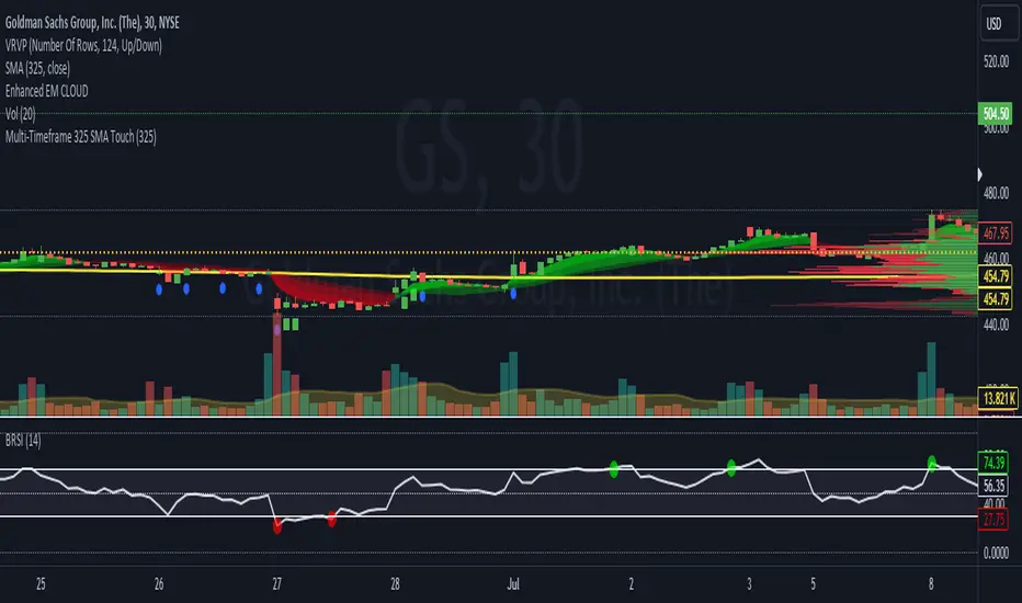
Multi-Timeframe 325 SMA TouchMulti-Timeframe 325 SMA Touch Indicator
This versatile indicator detects and visualizes when the price touches (crosses over or under) the 325-period Simple Moving Average (SMA) across multiple timeframes. It's designed to help traders identify potential support and resistance levels across various time horizons.
Key Features:
Monitors 7 different timeframes: 30 minutes, 1 hour, 2 hours, 4 hours, 6 hours, 12 hours, and 1 day.
Customizable: Each timeframe can be toggled on or off individually.
Visual cues: Unique shapes and colors for each timeframe make it easy to distinguish touches on different time scales.
Adjustable SMA length: While defaulted to 325 periods, the SMA length can be modified to suit your strategy.
Current timeframe SMA: Displays the 325 SMA on the chart for additional context.
How it Works:
The indicator checks for price touches on the 325 SMA for each selected timeframe. When a touch occurs, it plots a distinct shape below the price bar:
30 minutes: Blue circle
1 hour: Green square
2 hours: Red triangle (up)
4 hours: Purple diamond
6 hours: Teal triangle (down)
12 hours: Orange X
1 day: White circle
The 325 SMA for the current chart timeframe is also plotted as a yellow line for reference.
Use Cases:
Identify potential support and resistance levels across multiple timeframes
Spot confluences where touches occur on multiple timeframes simultaneously
Enhance your multi-timeframe analysis for more informed trading decisions
Use as a filter or confirmation tool in your existing trading strategy
Customization:
You can easily customize the indicator by adjusting the SMA length or toggling specific timeframes on/off to focus on the time horizons most relevant to your trading style.
Daily Levels Percentual [TOLK] Settings Crypto and ForexPercentage zones refer to specific areas or bands on the price chart of a financial asset that are bounded by percentages of change relative to a reference point, such as the opening price or a reference value from a previous move.
These zones are useful for identifying support and resistance levels, predicting possible price reversals, or setting price targets. For example, on a price chart, you can create percentage zones to observe how the price behaves when it reaches 1%, 2%, 5%, 10%, etc., above or below a certain point.
These zones can be used in conjunction with other technical analysis tools, such as Fibonacci, moving averages, or volume analysis, to improve decision-making in trading strategies.
The default indicator levels are as follows:
SETTINGS Crypto:
Crypto Level 1 > 1.0%
Crypto Level 2 > 1.618%
Crypto Level 3 > 2.0%
Crypto Level 4 > 2.618%
Crypto Level 5 > 3.618%
Crypto Level 6 > 4.618%
Crypto Level 7 > 5.0%
Crypto Level 8 > 7.618%
Crypto Level 9 > 10.0%
Crypto Level 10 > 12.618%
Crypto Level 11 > 13.618%
Crypto Level 12 > 15%
Crypto Level 13 > 17.618%
Crypto Level 14 > 20%
SETTINGS Forex:
Forex Level 1 > 0.10%
Forex Level 2 > 0.1618%
Forex Level 3 > 0.20%
Forex Level 4 > 0.2618%
Forex Level 5 > 0.3618%
Forex Level 6 > 0.4618%
Forex Level 7 > 0.50%
Forex Level 8 > 0.7618%
Forex Level 9 > 1.0%
Forex Level 10 > 1.2618%
Forex Level 11 > 1.3618%
Forex Level 12 > 1.50%
Forex Level 13 > 1.7618%
Forex Level 14 > 2.0%
Percentage Levels This approach helps identify critical price levels where the asset may encounter support or resistance, making it easier to make trading decisions based on price movement patterns.

MNQ/NQ Rotations [Tiestobob]### Indicator Description: MNQ/NQ Rotations
TO BE USED ONLY ON THE CONTINOUS CONTRACTS NQ1! and MNQ1! It will not work on others or the forward contracts of these.
#### Overview
The MNQ/NQ Rotations indicator is designed for traders of Nasdaq futures (MNQ and NQ) to visualize key price levels where typical market rotations occur. This indicator identifies and highlights the xxx.20 and xxx.80 levels based on empirical data and trading experience, allowing traders to recognize potential support and resistance points during trading sessions.
#### Key Features
- **Timeframe Selection**: The indicator allows users to specify a timeframe for identifying breakout candles, ensuring flexibility across different trading strategies.
- **Active Trading Range**: Users can define an active trading range, focusing the analysis on specific hours when the market is most active.
- **Visual Representation**: The indicator paints horizontal lines at key price levels (xxx.20 and xxx.80), extending them across a user-defined length to aid in visual analysis.
- **Customization**: Users can customize the color of the lines to match their charting preferences.
#### Inputs
- **Timeframe (`tf`)**: Defines the timeframe to select the breakout candle (default: 1 minute).
- **Active Trading Range (`session`)**: Specifies the time range for identifying breakout candles (default: 08:00-12:00).
- **Line Color (`line_color`)**: Allows customization of the line color (default: purple).
#### Logic
1. **Session Validation**: The indicator checks if the current bar falls within the specified active trading range.
2. **Price Point Calculation**: For each candle close, the indicator calculates the nearest xxx.20 and xxx.80 levels.
3. **Line Drawing**: Horizontal lines are drawn at these key levels, extending a specified length forward to highlight potential rotation points.
#### Use Cases
- **Support and Resistance Identification**: By highlighting the xxx.20 and xxx.80 levels, traders can easily spot areas where the market is likely to reverse or consolidate.
- **Breakout Trading**: Traders can use the indicator to identify breakout levels and set appropriate entry points.
- **Risk Management**: The visual cues provided by the indicator can help traders set more effective stop-loss and take-profit levels.
#### Example
A trader using a 1-minute timeframe with an active trading range from 08:00 to 12:00 will see horizontal lines painted at the nearest xxx.20 and xxx.80 levels for each candle close during this period. These lines serve as visual markers for typical rotation points, aiding in decision-making and trade planning.
#### Conclusion
The MNQ/NQ Rotations indicator is a powerful tool for traders looking to enhance their market analysis of Nasdaq futures. By focusing on empirically derived rotation levels, this indicator provides clear visual cues for identifying key price levels, supporting more informed trading decisions.
Ripster MTF CloudsDescription:
MTF EMA Cloud By Ripster
EMA Cloud System is a Trading System Invented by Ripster where areas are shaded between two desired EMAs. The concept implies the EMA cloud area serves as support or resistance for Intraday & Swing Trading. This can be utilized effectively on 10 Min for day trading and 1Hr/Daily for Swings. Ripster himself utilizes various combinations of the 5-12, 34-50, 8-9, 20-21 EMA clouds but the possibilities are endless to find what works best for you.
“Ideally, 5-12 or 5-13 EMA cloud acts as a fluid trendline for day trades. 8-9 EMA Clouds can be used as pullback Levels –(optional). Additionally, a high level price over or under 34-50 EMA clouds confirms either bullish or bearish bias on the price action for any timeframe” – Ripster
This indicator is an extension of the Ripster EMA Clouds. It allows you to visualize Exponential Moving Average (EMA) clouds from any time frame on your current chart, regardless of the chart's own time frame. This functionality is especially useful for traders who want to monitor higher time frame trends and support/resistance levels while trading on lower time frames.
What does this code do?
The Ripster MTF Clouds indicator displays two sets of EMA clouds. Each set consists of a short EMA and a long EMA. By default, the indicator uses Daily 20/21 and 50/55 EMAs, but you can customize these settings to fit your trading strategy. The EMAs are plotted on your chart along with their corresponding clouds, colored for easy differentiation:
EMA 1 (default 50/55): Plotted in blue.
EMA 2 (default 20/21): Plotted in teal.
The indicator uses the security function to fetch EMA values from higher time frames and plots them on your current chart, allowing you to see how these higher time frame EMAs interact with your current time frame's price action.
How to use this indicator:
Adjust Resolution:
Set the "Resolution" input to the time frame from which you want to fetch EMA values. For example, set it to "1H" if you want to see 1-hour EMAs on your current chart.
Customize EMAs:
Modify the "EMA 1 Short Length" and "EMA 1 Long Length" inputs to change the default 50/55 EMAs.
Adjust the "EMA 2 Short Length" and "EMA 2 Long Length" inputs to change the default 20/21 EMAs.
Monitor Clouds:
The indicator fills the area between the short and long EMAs, creating a cloud that helps visualize the trend. A blue cloud indicates the area between the EMA 1 pair, while a teal cloud indicates the area between the EMA 2 pair.
Use Multiple Instances:
You can add multiple instances of this indicator to your chart to monitor multiple higher time frames simultaneously. For instance, one instance can show daily clouds while another shows hourly clouds.
Integration with Trading Strategy:
Use this indicator to identify higher time frame trends and support/resistance levels, which can help improve your trading decisions on lower time frames.
For example, you can go long when the stock is above the 50-55 EMA clouds and 20-21 EMA clouds with daily resolution on a 10-minute chart and short when it is below it.
Similarly, you can short a stock under the 1-hour 34/50 EMA clouds while still trading on a 10-minute chart.
Pivot Points Level [TradingFinder] 4 Methods + Reversal lines🔵 Introduction
"Pivot Points" are places on the price chart where buyers and sellers are most active. Pivot points are calculated based on the previous day's price data and serve as reference points for traders to make decisions.
Types of Pivot Points :
Floor
Woodie
Camarilla
Fibonacci
🟣 Floor Pivot Points
Floor pivot points are widely used in technical analysis. The central pivot point (PP) serves as the main level of support or resistance, indicating the potential direction of the trend.
The first to third levels of resistance (R1, R2, R3) and support (S1, S2, S3) provide additional signals for potential trend reversals or continuations.
Floor Pivot Points Formula :
Pivot Point (PP): (H + L + C) / 3
First Resistance (R1): (2 * P) - L
Second Resistance (R2): P + H - L
Third Resistance (R3): H + 2 * (P - L)
First Support (S1): (2 * P) - H
Second Support (S2): P - H + L
Third Support (S3): L - 2 * (H - P)
🟣 Camarilla Pivot Points
Camarilla pivot points include eight levels that closely align with support and resistance. These points are particularly useful for setting stop-loss and profit targets.
Camarilla Pivot Points Formula :
Fourth Resistance (R4): (H - L) * 1.1 / 2 + C
Third Resistance (R3): (H - L) * 1.1 / 4 + C
Second Resistance (R2): (H - L) * 1.1 / 6 + C
First Resistance (R1): (H - L) * 1.1 / 12 + C
First Support (S1): C - (H - L) * 1.1 / 12
Second Support (S2): C - (H - L) * 1.1 / 6
Third Support (S3): C - (H - L) * 1.1 / 4
Fourth Support (S4): C - (H - L) * 1.1 / 2
🟣 Woodie Pivot Points
Woodie pivot points are similar to floor pivot points but place more emphasis on the closing price. This method often results in different pivot levels than the floor method.
Woodie Pivot Points Formula :
Pivot Point (PP): (H + L + 2 * C) / 4
First Resistance (R1): (2 * P) - L
Second Resistance (R2): P + H - L
First Support (S1): (2 * P) - H
Second Support (S2): P - H + L
🟣 Fibonacci Pivot Points
Fibonacci pivot points use the standard floor pivot points and then apply Fibonacci retracement levels to the range of the previous trading period. The common retracement levels used are 38.2%, 61.8%, and 100%.
Fibonacci Pivot Points Formula :
Pivot Point (PP): (H + L + C) / 3
Third Resistance (R3): PP + ((H - L) * 1.000)
Second Resistance (R2): PP + ((H - L) * 0.618)
First Resistance (R1): PP + ((H - L) * 0.382)
First Support (S1): PP - ((H - L) * 0.382)
Second Support (S2): PP - ((H - L) * 0.618)
Third Support (S3): PP - ((H - L) * 1.000)
These pivot point calculations help traders identify potential support and resistance levels, enabling more informed decision-making in their trading strategies.
🔵 How to Use
🟣 Two Methods for Trading Pivot Points
There are two primary methods for trading pivot points: trading with "pivot point breakouts" and trading with "price reversals."
🟣 Pivot Point Breakout
A breakout through pivot lines provides a significant signal to the trader, indicating a change in market sentiment. When an upward breakout occurs and the price crosses these lines, a trader can enter a long position and place their stop-loss below the pivot point (P).
Similarly, if a downward breakout happens, a short order can be placed below the pivot point.
When trading with pivot point breakouts, if the upward trend breaks, the first and second support levels can be the trader's profit targets. In a downward trend, the first and second resistance levels will serve this role.
🟣 Price Reversal
Another method for trading pivot points is waiting for the price to reverse from the support and resistance levels. To execute this strategy, one should trade in the opposite direction of the trend as the price reverses from the pivot point.
It's worth noting that although traders use this tool in higher time frames, it yields better results in shorter time frames such as one-hour, 30-minute, and 15-minute intervals.

Daye's Quarterly TheoryDaye's Quarterly Theory Indicator
Description
The Daye's Quarterly Theory Indicator divides trading time into smaller units to help traders identify potential accumulation, manipulation, distribution, and reversal/continuation phases within a day. It applies these time divisions to your charts, offering visual guidance aligned with ICT's PO3 concept:
Accumulation (A): The phase where positions are accumulated.
Manipulation (M): The phase where the market moves against the prevailing trend to trap traders.
Distribution (D): The phase where accumulated positions are distributed.
Reversal/Continuation (X): The phase indicating either a reversal or continuation of the trend.
This indicator breaks down time into quarters at different levels:
Daily Quarters:
Q1: 18:00 - 00:00 (Asia)
Q2: 00:00 - 06:00 (London)
Q3: 06:00 - 12:00 (NY AM)
Q4: 12:00 - 18:00 (NY PM)
90-Minute Quarters:
Q1: 18:00 - 19:30
Q2: 19:30 - 21:00
Q3: 21:00 - 22:30
Q4: 22:30 - 00:00
Micro Quarters (22.5 minutes) (Displayed on 7-minute TF or lower):
Q1: 18:00 - 18:22:30
Q2: 18:22:30 - 18:45
Q3: 18:45 - 19:07:30
Q4: 19:07:30 - 19:30
Features
Time Box Visualization: Highlights different quarters of the trading day to help visualize market phases.
Customizable Colors: Allows users to set different colors for daily, 90-minute, and micro quarters.
Flexible Settings: Designed to work out-of-the-box on both light and dark background charts.
ICT PO3 Alignment: Helps traders align their strategies with ICT's Accumulation, Manipulation, Distribution, and Reversal/Continuation phases.
Usage
Apply this indicator to your NQ1! or ES1! charts and observe the confluence with ICT's macro times. Use it to predict potential market phases and optimize your trading strategy by buying after manipulation down or selling after manipulation up.
Note: The indicator's display may vary based on the timeframe viewed and broker feeds. Back-test and research for best results on your preferred assets.

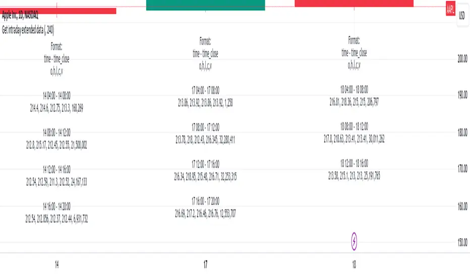
Get intraday extended dataIf you have interacted with Pine for some time, you probably noticed that if you are using DWM resolutions, you will not be able to obtain complete data from the extended intraday ticker using the usual functions request.security() and request.security_lower_tf(). This is quite logical if you understand the principle of mapping data from the secure context to the main one. The main reason is the different opening and closing times of the intraday data with extended clocks and DWM.
This script visualizes one of the approaches to solving this problem. I will briefly describe the principle of operation:
For example, take the symbol NASDAQ:AAPL.
Our main resolution is 1D, but we want to receive extended data from a 4-hour interval. The daytime bar opens at 09:30 and closes at 16:00. The same period at a resolution of 4 hours covers 4 bars:
04:00 - 08:00
08:00 - 12:00
12:00 - 16:00
16:00 - 20:00
So, if we use the request.security_lower_tf() function, we will not get the bars 04:00 - 08:00 and 16:00 - 20:00 because their closing times are not within the range of the main context (09:30 - 16:00).
If we use the request.security() function, we will get the bar 04:00 - 08:00, but we will not get the bar 16:00 - 20:00 because its closing time will be in the future, and it is impossible to get values from the future.
So, what I propose is to use the upgraded request.security() function, inside which another function will be executed, storing all the bars in a var array and putting the post-market bars in the array of the next day. Next, all we have to do is isolate these bars, place them in the previous array, and remove them from the current one.
I visualized the received data simply as text, but you can do it differently using the proposed mechanism.
In order for everything to work, you need to fill in the inputs correctly:
"Symbol for calculate" - This is the symbol from which we will receive extended data.
"Intraday data period" - The period from which we will receive extended data.
"Specify your chart timeframe here" - This is an input that allows you to operate with data from the main context while being inside the secure one. Enter your current chart timeframe here. If there are problems, a warning will appear informing you about this.
If you want to use these developments, take the get_data() function, it will return:
1. the number of past items - it is useful for outputting values in real time, because it is not possible to simply delete them there, because they will always arrive and it is easier to make a slice with an indentation for this number
2. cleared object of type Inner_data containing arrays of open, high, low, close, volume, time, time_close intraday data
3. its same value from the previous bar
RiskMetrics█ OVERVIEW
This library is a tool for Pine programmers that provides functions for calculating risk-adjusted performance metrics on periodic price returns. The calculations used by this library's functions closely mirror those the Broker Emulator uses to calculate strategy performance metrics (e.g., Sharpe and Sortino ratios) without depending on strategy-specific functionality.
█ CONCEPTS
Returns, risk, and volatility
The return on an investment is the relative gain or loss over a period, often expressed as a percentage. Investment returns can originate from several sources, including capital gains, dividends, and interest income. Many investors seek the highest returns possible in the quest for profit. However, prudent investing and trading entails evaluating such returns against the associated risks (i.e., the uncertainty of returns and the potential for financial losses) for a clearer perspective on overall performance and sustainability.
One way investors and analysts assess the risk of an investment is by analyzing its volatility , i.e., the statistical dispersion of historical returns. Investors often use volatility in risk estimation because it provides a quantifiable way to gauge the expected extent of fluctuation in returns. Elevated volatility implies heightened uncertainty in the market, which suggests higher expected risk. Conversely, low volatility implies relatively stable returns with relatively minimal fluctuations, thus suggesting lower expected risk. Several risk-adjusted performance metrics utilize volatility in their calculations for this reason.
Risk-free rate
The risk-free rate represents the rate of return on a hypothetical investment carrying no risk of financial loss. This theoretical rate provides a benchmark for comparing the returns on a risky investment and evaluating whether its excess returns justify the risks. If an investment's returns are at or below the theoretical risk-free rate or the risk premium is below a desired amount, it may suggest that the returns do not compensate for the extra risk, which might be a call to reassess the investment.
Since the risk-free rate is a theoretical concept, investors often utilize proxies for the rate in practice, such as Treasury bills and other government bonds. Conventionally, analysts consider such instruments "risk-free" for a domestic holder, as they are a form of government obligation with a low perceived likelihood of default.
The average yield on short-term Treasury bills, influenced by economic conditions, monetary policies, and inflation expectations, has historically hovered around 2-3% over the long term. This range also aligns with central banks' inflation targets. As such, one may interpret a value within this range as a minimum proxy for the risk-free rate, as it may correspond to the minimum rate required to maintain purchasing power over time.
The built-in Sharpe and Sortino ratios that strategies calculate and display in the Performance Summary tab use a default risk-free rate of 2%, and the metrics in this library's example code use the same default rate. Users can adjust this value to fit their analysis needs.
Risk-adjusted performance
Risk-adjusted performance metrics gauge the effectiveness of an investment by considering its returns relative to the perceived risk. They aim to provide a more well-rounded picture of performance by factoring in the level of risk taken to achieve returns. Investors can utilize such metrics to help determine whether the returns from an investment justify the risks and make informed decisions.
The two most commonly used risk-adjusted performance metrics are the Sharpe ratio and the Sortino ratio.
1. Sharpe ratio
The Sharpe ratio , developed by Nobel laureate William F. Sharpe, measures the performance of an investment compared to a theoretically risk-free asset, adjusted for the investment risk. The ratio uses the following formula:
Sharpe Ratio = (𝑅𝑎 − 𝑅𝑓) / 𝜎𝑎
Where:
• 𝑅𝑎 = Average return of the investment
• 𝑅𝑓 = Theoretical risk-free rate of return
• 𝜎𝑎 = Standard deviation of the investment's returns (volatility)
A higher Sharpe ratio indicates a more favorable risk-adjusted return, as it signifies that the investment produced higher excess returns per unit of increase in total perceived risk.
2. Sortino ratio
The Sortino ratio is a modified form of the Sharpe ratio that only considers downside volatility , i.e., the volatility of returns below the theoretical risk-free benchmark. Although it shares close similarities with the Sharpe ratio, it can produce very different values, especially when the returns do not have a symmetrical distribution, since it does not penalize upside and downside volatility equally. The ratio uses the following formula:
Sortino Ratio = (𝑅𝑎 − 𝑅𝑓) / 𝜎𝑑
Where:
• 𝑅𝑎 = Average return of the investment
• 𝑅𝑓 = Theoretical risk-free rate of return
• 𝜎𝑑 = Downside deviation (standard deviation of negative excess returns, or downside volatility)
The Sortino ratio offers an alternative perspective on an investment's return-generating efficiency since it does not consider upside volatility in its calculation. A higher Sortino ratio signifies that the investment produced higher excess returns per unit of increase in perceived downside risk.
█ CALCULATIONS
Return period detection
Calculating risk-adjusted performance metrics requires collecting returns across several periods of a given size. Analysts may use different period sizes based on the context and their preferences. However, two widely used standards are monthly or daily periods, depending on the available data and the investment's duration. The built-in ratios displayed in the Strategy Tester utilize returns from either monthly or daily periods in their calculations based on the following logic:
• Use monthly returns if the history of closed trades spans at least two months.
• Use daily returns if the trades span at least two days but less than two months.
• Do not calculate the ratios if the trade data spans fewer than two days.
This library's `detectPeriod()` function applies related logic to available chart data rather than trade data to determine which period is appropriate:
• It returns true if the chart's data spans at least two months, indicating that it's sufficient to use monthly periods.
• It returns false if the chart's data spans at least two days but not two months, suggesting the use of daily periods.
• It returns na if the length of the chart's data covers less than two days, signifying that the data is insufficient for meaningful ratio calculations.
It's important to note that programmers should only call `detectPeriod()` from a script's global scope or within the outermost scope of a function called from the global scope, as it requires the time value from the first bar to accurately measure the amount of time covered by the chart's data.
Collecting periodic returns
This library's `getPeriodicReturns()` function tracks price return data within monthly or daily periods and stores the periodic values in an array . It uses a `detectPeriod()` call as the condition to determine whether each element in the array represents the return over a monthly or daily period.
The `getPeriodicReturns()` function has two overloads. The first overload requires two arguments and outputs an array of monthly or daily returns for use in the `sharpe()` and `sortino()` methods. To calculate these returns:
1. The `percentChange` argument should be a series that represents percentage gains or losses. The values can be bar-to-bar return percentages on the chart timeframe or percentages requested from a higher timeframe.
2. The function compounds all non-na `percentChange` values within each monthly or daily period to calculate the period's total return percentage. When the `percentChange` represents returns from a higher timeframe, ensure the requested data includes gaps to avoid compounding redundant values.
3. After a period ends, the function queues the compounded return into the array , removing the oldest element from the array when its size exceeds the `maxPeriods` argument.
The resulting array represents the sequence of closed returns over up to `maxPeriods` months or days, depending on the available data.
The second overload of the function includes an additional `benchmark` parameter. Unlike the first overload, this version tracks and collects differences between the `percentChange` and the specified `benchmark` values. The resulting array represents the sequence of excess returns over up to `maxPeriods` months or days. Passing this array to the `sharpe()` and `sortino()` methods calculates generalized Information ratios , which represent the risk-adjustment performance of a sequence of returns compared to a risky benchmark instead of a risk-free rate. For consistency, ensure the non-na times of the `benchmark` values align with the times of the `percentChange` values.
Ratio methods
This library's `sharpe()` and `sortino()` methods respectively calculate the Sharpe and Sortino ratios based on an array of returns compared to a specified annual benchmark. Both methods adjust the annual benchmark based on the number of periods per year to suit the frequency of the returns:
• If the method call does not include a `periodsPerYear` argument, it uses `detectPeriod()` to determine whether the returns represent monthly or daily values based on the chart's history. If monthly, the method divides the `annualBenchmark` value by 12. If daily, it divides the value by 365.
• If the method call does specify a `periodsPerYear` argument, the argument's value supersedes the automatic calculation, facilitating custom benchmark adjustments, such as dividing by 252 when analyzing collected daily stock returns.
When the array passed to these methods represents a sequence of excess returns , such as the result from the second overload of `getPeriodicReturns()`, use an `annualBenchmark` value of 0 to avoid comparing those excess returns to a separate rate.
By default, these methods only calculate the ratios on the last available bar to minimize their resource usage. Users can override this behavior with the `forceCalc` parameter. When the value is true , the method calculates the ratio on each call if sufficient data is available, regardless of the bar index.
Look first. Then leap.
█ FUNCTIONS & METHODS
This library contains the following functions:
detectPeriod()
Determines whether the chart data has sufficient coverage to use monthly or daily returns
for risk metric calculations.
Returns: (bool) `true` if the period spans more than two months, `false` if it otherwise spans more
than two days, and `na` if the data is insufficient.
getPeriodicReturns(percentChange, maxPeriods)
(Overload 1 of 2) Tracks periodic return percentages and queues them into an array for ratio
calculations. The span of the chart's historical data determines whether the function uses
daily or monthly periods in its calculations. If the chart spans more than two months,
it uses "1M" periods. Otherwise, if the chart spans more than two days, it uses "1D"
periods. If the chart covers less than two days, it does not store changes.
Parameters:
percentChange (float) : (series float) The change percentage. The function compounds non-na values from each
chart bar within monthly or daily periods to calculate the periodic changes.
maxPeriods (simple int) : (simple int) The maximum number of periodic returns to store in the returned array.
Returns: (array) An array containing the overall percentage changes for each period, limited
to the maximum specified by `maxPeriods`.
getPeriodicReturns(percentChange, benchmark, maxPeriods)
(Overload 2 of 2) Tracks periodic excess return percentages and queues the values into an
array. The span of the chart's historical data determines whether the function uses
daily or monthly periods in its calculations. If the chart spans more than two months,
it uses "1M" periods. Otherwise, if the chart spans more than two days, it uses "1D"
periods. If the chart covers less than two days, it does not store changes.
Parameters:
percentChange (float) : (series float) The change percentage. The function compounds non-na values from each
chart bar within monthly or daily periods to calculate the periodic changes.
benchmark (float) : (series float) The benchmark percentage to compare against `percentChange` values.
The function compounds non-na values from each bar within monthly or
daily periods and subtracts the results from the compounded `percentChange` values to
calculate the excess returns. For consistency, ensure this series has a similar history
length to the `percentChange` with aligned non-na value times.
maxPeriods (simple int) : (simple int) The maximum number of periodic excess returns to store in the returned array.
Returns: (array) An array containing monthly or daily excess returns, limited
to the maximum specified by `maxPeriods`.
method sharpeRatio(returnsArray, annualBenchmark, forceCalc, periodsPerYear)
Calculates the Sharpe ratio for an array of periodic returns.
Callable as a method or a function.
Namespace types: array
Parameters:
returnsArray (array) : (array) An array of periodic return percentages, e.g., returns over monthly or
daily periods.
annualBenchmark (float) : (series float) The annual rate of return to compare against `returnsArray` values. When
`periodsPerYear` is `na`, the function divides this value by 12 to calculate a
monthly benchmark if the chart's data spans at least two months or 365 for a daily
benchmark if the data otherwise spans at least two days. If `periodsPerYear`
has a specified value, the function divides the rate by that value instead.
forceCalc (bool) : (series bool) If `true`, calculates the ratio on every call. Otherwise, ratio calculation
only occurs on the last available bar. Optional. The default is `false`.
periodsPerYear (simple int) : (simple int) If specified, divides the annual rate by this value instead of the value
determined by the time span of the chart's data.
Returns: (float) The Sharpe ratio, which estimates the excess return per unit of total volatility.
method sortinoRatio(returnsArray, annualBenchmark, forceCalc, periodsPerYear)
Calculates the Sortino ratio for an array of periodic returns.
Callable as a method or a function.
Namespace types: array
Parameters:
returnsArray (array) : (array) An array of periodic return percentages, e.g., returns over monthly or
daily periods.
annualBenchmark (float) : (series float) The annual rate of return to compare against `returnsArray` values. When
`periodsPerYear` is `na`, the function divides this value by 12 to calculate a
monthly benchmark if the chart's data spans at least two months or 365 for a daily
benchmark if the data otherwise spans at least two days. If `periodsPerYear`
has a specified value, the function divides the rate by that value instead.
forceCalc (bool) : (series bool) If `true`, calculates the ratio on every call. Otherwise, ratio calculation
only occurs on the last available bar. Optional. The default is `false`.
periodsPerYear (simple int) : (simple int) If specified, divides the annual rate by this value instead of the value
determined by the time span of the chart's data.
Returns: (float) The Sortino ratio, which estimates the excess return per unit of downside
volatility.

Hybrid Overbought/Oversold OverlayIntroduction
This is a new representation of my well-known oscillator Hybrid Overbought/Oversold Detector overlaid on the chart. The script utilizes the following 12 different oscillators to bring forth a new indicator which I call it Hybrid OB/OS .
Utilized Oscillators
The utilized oscillators here are:
Bollinger Bands %B
Chaikin Money Flow (CMF)
Chande Momentum Oscillator (CMO)
Commodity Channel Index (CCI)
Disparity Index (DIX)
Keltner Channel %K
Money Flow Index (MFI)
Rate Of Change (ROC)
Relative Strength Index (RSI)
Relative Vigor Index (RVI/RVGI)
Stochastic
Twiggs Money Flow (TMF)
The challenging part of utilizing mentioned oscillators was that some of their formulas range are not similar and some of them does not have a mathematical range at all. So I used a normalization function to normalize all their output values to (0, 100) interval.
Overbought/Oversold Levels Calculation
I noticed that the levels which considered as OB/OS level by various traders for each of the utilized oscillators are so different, e.g., many traders consider 30 as OS level and 70 as OB level for RSI and some others take 20 and 80 as the levels, or some traders consider 20 and 80 as OS/OB levels for Stochastic oscillator. Also these levels could be different on different assets, e.g., OB/OS levels for CCI on EURUSD chart might be 80 and 20 while the levels on BTCUSDT chart might be 75 and 25, and so on.
So I decided to make a routine to automate the calculation of these levels using historical data. By this feature, my indicator would calculate the corresponding levels for the oscillators on current chart and then decide about the overbought/oversold situation of each one, which leads to a more accurate Hybrid OB/OS indication.
As the result, if all 12 individual oscillators say it's overbought/oversold, the Hybrid OB/OS shows 100% overbought/oversold, vice versa, if none of them say it's overbought/oversold, the Hybrid OB/OS shows 0, and so on.
The Overlaying Oscillator Problem!
A programming-related challenge here was that Pine Script assigns two separate spaces to the oscillators and the overlaid indicators, and the programmers are limited to use just one of them in each of their codes.
Knowing this, I was forced to simulate the oscillator space on the chart and display my oscillator as a diagram somehow. Of course it won't be as nice as the oscillator itself, because the relation between the main chart bars and the oscillator bars could not be obtained, but it's better than nothing!
Settings and Usage
The indicator settings contain some options about the calculations, the diagram display and the signals appearance. By default they are fine, but you could change them as you prefer.
This indicator is better to be used alongside other indicators as a confirmation (specially in counter-trend strategies I believe). Also it generates an external signal which you could use it in your own designed indicators as well.
Feel free to test it and also the former form of the Hybrid OB/OS . Good Luck!
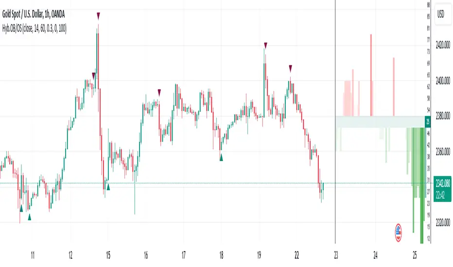
Earnings Line+Growth stock investors are concerned with Earnings per share that is growing, Sales (Revenue) that is growing and Increasing gross margins. This indicator helps view each of these parameters.
On the chart is Tesla (TSLA) gross margin (blue line) on a 12 trailing months basis (TTM). As you can see, TSLA's margins appear to be eroding.
The user selects one of the following parameters to display from the input drop down menu:
"EARNINGS_PER_SHARE_BASIC", "TOTAL_REVENUE", or "GROSS_MARGIN".
The value axis for your selection will appear on the left side of the chart.
The user also selects one of the following periods: "FY", "FQ" or "TTM" (Fiscal year, fiscal quarter or 12-trailing months). You have an option to display the inputs by checking the box. This is useful as a reminder but can be removed if the label is in the way.
The chart will render on any chart time scale, however longer time scales will probably be of more value. Weekly charts work well.
It is not possible to display more than one line simultaneously because of axis incompatibilities. However, it is possible to load this indicator multiple times and select different items in each. In this case additional left-side scales will be shown as well as additional lines. Common pairings are Revenue (Sales) and Earnings, or, Revenue and Gross Margin.
@ jmikes

LMACD - Logarithmic MACD Weekly BTC Index [Logue]Logarithmic Moving Average Convergence Divergence (LMACD) Weekly Indicator - The LMACD is a momentum indicator that measures the strength of a trend using 12-period and 26-period moving averages. The weekly LMACD for this indicator is calculated by determining the difference between the log (base 10) of the 12-week and 26-week exponential moving averages. Larger positive numbers indicate a larger positive momentum.
For tops: The default setting for tops is based on decreasing "strength" of BTC tops. A decreasing linear function (trigger = slope * time + intercept) was fit to past cycle tops for this indicator and is used as the default to signal macro tops. The user can change the slope and intercept of the line by changing the slope and/or intercept factor. The user also has the option to indicate tops based on a horizontal line via a settings selection. This line default value is 0.125. This indicator is triggered for a top when the LMACD is above the trigger value.
For bottoms: Bottoms are displayed based on a horizontal line with a default setting of -0.07. The indicator is triggered for a bottom when the LMACD is below the bottom trigger value.

Moving Average PropertiesThis indicator calculates and visualizes the Relative Smoothness (RS) and Relative Lag (RL) or call it accuracy of a selected moving average (MA) in comparison to the SMA of length 2 (the lowest possible length for a moving average and also the one closest to the price).
Median RS (Relative Smoothness):
Interpretation: The median RS represents the median value of the Relative Smoothness calculated for the selected moving average across a specified look-back period (max bar lookback is set at 3000).
Significance: A more negative (larger) median RS suggests that the chosen moving average has exhibited smoother price behavior compared to a simple moving average over the analyzed period. A less negative value indicates a relatively choppier price movement.
Median RL (Relative Lag):
Interpretation: The median RL represents the median value of the Relative Lag calculated for the selected moving average compared to a simple moving average of length 2.
Significance: A higher median RL indicates that the chosen moving average tends to lag more compared to a simple moving average. Conversely, lower values suggest less lag in the selected moving average.
Ratio of Median RS to Median RL:
Interpretation: This ratio is calculated by dividing the median RS by the median RL.
Significance: Traders might use this ratio to assess the balance between smoothness and lag in the chosen moving average. This a measure of for every % of lag what is the smoothness achieved. This can be used a benchmark to decide what length to choose for a MA to get an equivalent value between two stocks. For example a TESLA stock on a 15 minute time frame with a length of 12 has a value (ratio of RS/RL) of -150 , where as APPLE stock of length 35 on a 15 minute chart also has a value (ratio of RS/RL) of -150.
I imply that a MA of length 12 working on TESLA stock is equivalent to MA of length 35 on a APPLE stock. (THIS IS A EXAMPLE).
My assumption is that finding the right moving average length for a stock isn't a one-size-fits-all situation. It's not just about using a fixed length; it's about adapting to the unique characteristics of each stock. I believe that what works for one stock might not work for another because they have different levels of smoothness or lag in their price movements. So, instead of applying the same length to all stocks, I suggest adjusting the length of the moving average to match the values that we know work best for achieving the desired smoothness or lag or its ratio (RS/RL). This way, we're customizing the indicator for each stock, tailoring it to their individual behaviors rather than sticking to a one-size-fits-all approach.
Users can choose from various types of moving averages (EMA, SMA, WMA, VWMA, HMA) and customize the length of the moving average. RS measures the smoothness of the MA, while RL measures its lag compared to a simple moving average. The script plots the median RS and RL values, the selected MA, and the ratio of median RS to median RL on the price chart. Traders can use this information to assess the performance of different moving averages and potentially inform their trading decisions.

Clustered Asset Moving Average @shrilssThe Clustered Asset Moving Average script is designed to provide traders with a unique perspective on a cluster of multiple assets. By combining the closing prices and volumes of 12 specified assets, this indicator calculates a Clustered Moving Average to reveal potential trends and market sentiment within this asset cluster.
Key Features:
- Asset Cluster Analysis:
The script considers 12 assets, including well-known names such as Google (GOOG), Microsoft (MSFT), Apple (AAPL), Tesla (TSLA), and others.
It calculates the price and volume of each asset to form a comprehensive view of the asset cluster.
- Clustered Moving Average Calculation:
The Asset Price and Volume are combined to calculate the Clustered Moving Average
This moving average reflects the relationship between the aggregated price and volume of the specified assets.
- Multiple Exponential Moving Averages (EMA):
The script includes three EMAs (10, 25, and 100) applied to the Clustered Moving Average, providing different time perspectives.
Users can customize the visibility of each EMA based on their trading preferences.
- Visual Representation:
The indicator offers a visual representation of the Clustered Moving Average, allowing traders to quickly identify trends and potential reversal points.
Different EMAs are color-coded, enhancing visual clarity.
HolidayLibrary "Holiday"
- Full Control over Holidays and Daylight Savings Time (DLS)
The Holiday Library is an essential tool for traders and analysts who engage in backtesting and live trading . This comprehensive library enables the incorporation of crucial calendar elements - specifically Daylight Savings Time (DLS) adjustments and public holidays - into trading strategies and backtesting environments.
Key Features:
- DLS Adjustments: The library takes into account the shifts in time due to Daylight Savings. This feature is particularly vital for backtesting strategies, as DLS can impact trading hours, which in turn affects the volatility and liquidity in the market. Accurate DLS adjustments ensure that backtesting scenarios are as close to real-life conditions as possible.
- Comprehensive Holiday Metadata: The library includes a rich set of holiday metadata, allowing for the detailed scheduling of trading activities around public holidays. This feature is crucial for avoiding skewed results in backtesting, where holiday trading sessions might differ significantly in terms of volume and price movement.
- Customizable Holiday Schedules: Users can add or remove specific holidays, tailoring the library to fit various regional market schedules or specific trading requirements.
- Visualization Aids: The library supports on-chart labels, making it visually intuitive to identify holidays and DLS shifts directly on trading charts.
Use Cases:
1. Strategy Development: When developing trading strategies, it’s important to account for non-trading days and altered trading hours due to holidays and DLS. This library enables a realistic and accurate representation of these factors.
2. Risk Management: Trading around holidays can be riskier due to thinner liquidity and greater volatility. By integrating holiday data, traders can better manage their risk exposure.
3. Backtesting Accuracy: For backtesting to be effective, it must simulate the actual market conditions as closely as possible. Incorporating holidays and DLS adjustments contributes to more reliable and realistic backtesting results.
4. Global Trading: For traders active in multiple global markets, this library provides an easy way to handle different holiday schedules and DLS shifts across regions.
The Holiday Library is a versatile tool that enhances the precision and realism of trading simulations and strategy development . Its integration into the trading workflow is straightforward and beneficial for both novice and experienced traders.
EasterAlgo(_year)
Calculates the date of Easter Sunday for a given year using the Anonymous Gregorian algorithm.
`Gauss Algorithm for Easter Sunday` was developed by the mathematician Carl Friedrich Gauss
This algorithm is based on the cycles of the moon and the fact that Easter always falls on the first Sunday after the first ecclesiastical full moon that occurs on or after March 21.
While it's not considered to be 100% accurate due to rare exceptions, it does give the correct date in most cases.
It's important to note that Gauss's formula has been found to be inaccurate for some 21st-century years in the Gregorian calendar. Specifically, the next suggested failure years are 2038, 2051.
This function can be used for Good Friday (Friday before Easter), Easter Sunday, and Easter Monday (following Monday).
en.wikipedia.org
Parameters:
_year (int) : `int` - The year for which to calculate the date of Easter Sunday. This should be a four-digit year (YYYY).
Returns: tuple - The month (1-12) and day (1-31) of Easter Sunday for the given year.
easterInit()
Inits the date of Easter Sunday and Good Friday for a given year.
Returns: tuple - The month (1-12) and day (1-31) of Easter Sunday and Good Friday for the given year.
isLeapYear(_year)
Determine if a year is a leap year.
Parameters:
_year (int) : `int` - 4 digit year to check => YYYY
Returns: `bool` - true if input year is a leap year
method timezoneHelper(utc)
Helper function to convert UTC time.
Namespace types: series int, simple int, input int, const int
Parameters:
utc (int) : `int` - UTC time shift in hours.
Returns: `string`- UTC time string with shift applied.
weekofmonth()
Function to find the week of the month of a given Unix Time.
Returns: number - The week of the month of the specified UTC time.
dayLightSavingsAdjustedUTC(utc, adjustForDLS)
dayLightSavingsAdjustedUTC
Parameters:
utc (int) : `int` - The normal UTC timestamp to be used for reference.
adjustForDLS (bool) : `bool` - Flag indicating whether to adjust for daylight savings time (DLS).
Returns: `int` - The adjusted UTC timestamp for the given normal UTC timestamp.
getDayOfYear(monthOfYear, dayOfMonth, weekOfMonth, dayOfWeek, lastOccurrenceInMonth, holiday)
Function gets the day of the year of a given holiday (1-366)
Parameters:
monthOfYear (int)
dayOfMonth (int)
weekOfMonth (int)
dayOfWeek (int)
lastOccurrenceInMonth (bool)
holiday (string)
Returns: `int` - The day of the year of the holiday 1-366.
method buildMap(holidayMap, holiday, monthOfYear, weekOfMonth, dayOfWeek, dayOfMonth, lastOccurrenceInMonth, closingTime)
Function to build the `holidaysMap`.
Namespace types: map
Parameters:
holidayMap (map) : `map` - The map of holidays.
holiday (string) : `string` - The name of the holiday.
monthOfYear (int) : `int` - The month of the year of the holiday.
weekOfMonth (int) : `int` - The week of the month of the holiday.
dayOfWeek (int) : `int` - The day of the week of the holiday.
dayOfMonth (int) : `int` - The day of the month of the holiday.
lastOccurrenceInMonth (bool) : `bool` - Flag indicating whether the holiday is the last occurrence of the day in the month.
closingTime (int) : `int` - The closing time of the holiday.
Returns: `map` - The updated map of holidays
holidayInit(addHolidaysArray, removeHolidaysArray, defaultHolidays)
Initializes a HolidayStorage object with predefined US holidays.
Parameters:
addHolidaysArray (array) : `array` - The array of additional holidays to be added.
removeHolidaysArray (array) : `array` - The array of holidays to be removed.
defaultHolidays (bool) : `bool` - Flag indicating whether to include the default holidays.
Returns: `map` - The map of holidays.
Holidays(utc, addHolidaysArray, removeHolidaysArray, adjustForDLS, displayLabel, defaultHolidays)
Main function to build the holidays object, this is the only function from this library that should be needed. \
all functionality should be available through this function. \
With the exception of initializing a `HolidayMetaData` object to add a holiday or early close. \
\
**Default Holidays:** \
`DLS begin`, `DLS end`, `New Year's Day`, `MLK Jr. Day`, \
`Washington Day`, `Memorial Day`, `Independence Day`, `Labor Day`, \
`Columbus Day`, `Veterans Day`, `Thanksgiving Day`, `Christmas Day` \
\
**Example**
```
HolidayMetaData valentinesDay = HolidayMetaData.new(holiday="Valentine's Day", monthOfYear=2, dayOfMonth=14)
HolidayMetaData stPatricksDay = HolidayMetaData.new(holiday="St. Patrick's Day", monthOfYear=3, dayOfMonth=17)
HolidayMetaData addHolidaysArray = array.from(valentinesDay, stPatricksDay)
string removeHolidaysArray = array.from("DLS begin", "DLS end")
܂Holidays = Holidays(
܂ utc=-6,
܂ addHolidaysArray=addHolidaysArray,
܂ removeHolidaysArray=removeHolidaysArray,
܂ adjustForDLS=true,
܂ displayLabel=true,
܂ defaultHolidays=true,
܂ )
plot(Holidays.newHoliday ? open : na, title="newHoliday", color=color.red, linewidth=4, style=plot.style_circles)
```
Parameters:
utc (int) : `int` - The UTC time shift in hours
addHolidaysArray (array) : `array` - The array of additional holidays to be added
removeHolidaysArray (array) : `array` - The array of holidays to be removed
adjustForDLS (bool) : `bool` - Flag indicating whether to adjust for daylight savings time (DLS)
displayLabel (bool) : `bool` - Flag indicating whether to display a label on the chart
defaultHolidays (bool) : `bool` - Flag indicating whether to include the default holidays
Returns: `HolidayObject` - The holidays object | Holidays = (holidaysMap: map, newHoliday: bool, holiday: string, dayString: string)
HolidayMetaData
HolidayMetaData
Fields:
holiday (series string) : `string` - The name of the holiday.
dayOfYear (series int) : `int` - The day of the year of the holiday.
monthOfYear (series int) : `int` - The month of the year of the holiday.
dayOfMonth (series int) : `int` - The day of the month of the holiday.
weekOfMonth (series int) : `int` - The week of the month of the holiday.
dayOfWeek (series int) : `int` - The day of the week of the holiday.
lastOccurrenceInMonth (series bool)
closingTime (series int) : `int` - The closing time of the holiday.
utc (series int) : `int` - The UTC time shift in hours.
HolidayObject
HolidayObject
Fields:
holidaysMap (map) : `map` - The map of holidays.
newHoliday (series bool) : `bool` - Flag indicating whether today is a new holiday.
activeHoliday (series bool) : `bool` - Flag indicating whether today is an active holiday.
holiday (series string) : `string` - The name of the holiday.
dayString (series string) : `string` - The day of the week of the holiday.