Ultimate Oscillator Trading StrategyThe Ultimate Oscillator Trading Strategy implemented in Pine Script™ is based on the Ultimate Oscillator (UO), a momentum indicator developed by Larry Williams in 1976. The UO is designed to measure price momentum over multiple timeframes, providing a more comprehensive view of market conditions by considering short-term, medium-term, and long-term trends simultaneously. This strategy applies the UO as a mean-reversion tool, seeking to capitalize on temporary deviations from the mean price level in the asset’s movement (Williams, 1976).
Strategy Overview:
Calculation of the Ultimate Oscillator (UO):
The UO combines price action over three different periods (short-term, medium-term, and long-term) to generate a weighted momentum measure. The default settings used in this strategy are:
Short-term: 6 periods (adjustable between 2 and 10).
Medium-term: 14 periods (adjustable between 6 and 14).
Long-term: 20 periods (adjustable between 10 and 20).
The UO is calculated as a weighted average of buying pressure and true range across these periods. The weights are designed to give more emphasis to short-term momentum, reflecting the short-term mean-reversion behavior observed in financial markets (Murphy, 1999).
Entry Conditions:
A long position is opened when the UO value falls below 30, indicating that the asset is potentially oversold. The value of 30 is a common threshold that suggests the price may have deviated significantly from its mean and could be due for a reversal, consistent with mean-reversion theory (Jegadeesh & Titman, 1993).
Exit Conditions:
The long position is closed when the current close price exceeds the previous day’s high. This rule captures the reversal and price recovery, providing a defined point to take profits.
The use of previous highs as exit points aligns with breakout and momentum strategies, as it indicates sufficient strength for a price recovery (Fama, 1970).
Scientific Basis and Rationale:
Momentum and Mean-Reversion:
The strategy leverages two well-established phenomena in financial markets: momentum and mean-reversion. Momentum, identified in earlier studies like those by Jegadeesh and Titman (1993), describes the tendency of assets to continue in their direction of movement over short periods. Mean-reversion, as discussed by Poterba and Summers (1988), indicates that asset prices tend to revert to their mean over time after short-term deviations. This dual approach aims to buy assets when they are temporarily oversold and capitalize on their return to the mean.
Multi-timeframe Analysis:
The UO’s incorporation of multiple timeframes (short, medium, and long) provides a holistic view of momentum, unlike single-period oscillators such as the RSI. By combining data across different timeframes, the UO offers a more robust signal and reduces the risk of false entries often associated with single-period momentum indicators (Murphy, 1999).
Trading and Market Efficiency:
Studies in behavioral finance, such as those by Shiller (2003), show that short-term inefficiencies and behavioral biases can lead to overreactions in the market, resulting in price deviations. This strategy seeks to exploit these temporary inefficiencies, using the UO as a signal to identify potential entry points when the market sentiment may have overly pushed the price away from its average.
Strategy Performance:
Backtests of this strategy show promising results, with profit factors exceeding 2.5 when the default settings are optimized. These results are consistent with other studies on short-term trading strategies that capitalize on mean-reversion patterns (Jegadeesh & Titman, 1993). The use of a dynamic, multi-period indicator like the UO enhances the strategy’s adaptability, making it effective across different market conditions and timeframes.
Conclusion:
The Ultimate Oscillator Trading Strategy effectively combines momentum and mean-reversion principles to trade on temporary market inefficiencies. By utilizing multiple periods in its calculation, the UO provides a more reliable and comprehensive measure of momentum, reducing the likelihood of false signals and increasing the profitability of trades. This aligns with modern financial research, showing that strategies based on mean-reversion and multi-timeframe analysis can be effective in capturing short-term price movements.
References:
Fama, E. F. (1970). Efficient Capital Markets: A Review of Theory and Empirical Work. The Journal of Finance, 25(2), 383-417.
Jegadeesh, N., & Titman, S. (1993). Returns to Buying Winners and Selling Losers: Implications for Stock Market Efficiency. The Journal of Finance, 48(1), 65-91.
Murphy, J. J. (1999). Technical Analysis of the Financial Markets: A Comprehensive Guide to Trading Methods and Applications. New York Institute of Finance.
Poterba, J. M., & Summers, L. H. (1988). Mean Reversion in Stock Prices: Evidence and Implications. Journal of Financial Economics, 22(1), 27-59.
Shiller, R. J. (2003). From Efficient Markets Theory to Behavioral Finance. Journal of Economic Perspectives, 17(1), 83-104.
Williams, L. (1976). Ultimate Oscillator. Market research and technical trading analysis.
Cari dalam skrip untuk "10年期国债+交易单位+价格"

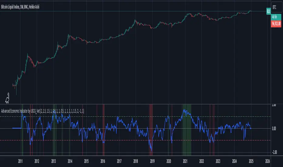
Advanced Economic Indicator by USCG_VetAdvanced Economic Indicator by USCG_Vet
tldr:
This comprehensive TradingView indicator combines multiple economic and financial metrics into a single, customizable composite index. By integrating key indicators such as the yield spread, commodity ratios, stock indices, and the Federal Reserve's QE/QT activities, it provides a holistic view of the economic landscape. Users can adjust the components and their weights to tailor the indicator to their analysis, aiding in forecasting economic conditions and market trends.
Detailed Description
Overview
The Advanced Economic Indicator is designed to provide traders and investors with a powerful tool to assess the overall economic environment. By aggregating a diverse set of economic indicators and financial market data into a single composite index, it helps identify potential turning points in the economy and financial markets.
Key Features:
Comprehensive Coverage: Includes 14 critical economic and financial indicators.
Customizable Components: Users can select which indicators to include.
Adjustable Weights: Assign weights to each component based on perceived significance.
Visual Signals: Clear plotting with threshold lines and background highlights.
Alerts: Set up alerts for when the composite index crosses user-defined thresholds.
Included Indicators
Yield Spread (10-Year Treasury Yield minus 3-Month Treasury Yield)
Copper/Gold Ratio
High Yield Spread (HYG/IEF Ratio)
Stock Market Performance (S&P 500 Index - SPX)
Bitcoin Performance (BLX)
Crude Oil Prices (CL1!)
Volatility Index (VIX)
U.S. Dollar Index (DXY)
Inflation Expectations (TIP ETF)
Consumer Confidence (XLY ETF)
Housing Market Index (XHB)
Manufacturing PMI (XLI ETF)
Unemployment Rate (Inverse SPY as Proxy)
Federal Reserve QE/QT Activities (Fed Balance Sheet - WALCL)
How to Use the Indicator
Configuring the Indicator:
Open Settings: Click on the gear icon (⚙️) next to the indicator's name.
Inputs Tab: You'll find a list of all components with checkboxes and weight inputs.
Including/Excluding Components
Checkboxes: Check or uncheck the box next to each component to include or exclude it from the composite index.
Default State: By default, all components are included.
Adjusting Component Weights:
Weight Inputs: Next to each component's checkbox is a weight input field.
Default Weights: Pre-assigned based on economic significance but fully adjustable.
Custom Weights: Enter your desired weight for each component to reflect your analysis.
Threshold Settings:
Bearish Threshold: Default is -1.0. Adjust to set the level below which the indicator signals potential economic downturns.
Bullish Threshold: Default is 1.0. Adjust to set the level above which the indicator signals potential economic upswings.
Setting the Timeframe:
Weekly Timeframe Recommended: Due to the inclusion of the Fed's balance sheet data (updated weekly), it's best to use this indicator on a weekly chart.
Changing Timeframe: Select 1W (weekly) from the timeframe options at the top of the chart.
Interpreting the Indicator:
Composite Index Line
Plot: The blue line represents the composite economic indicator.
Movement: Observe how the line moves relative to the threshold lines.
Threshold Lines
Zero Line (Gray Dotted): Indicates the neutral point.
Bearish Threshold (Red Dashed): Crossing below suggests potential economic weakness.
Bullish Threshold (Green Dashed): Crossing above suggests potential economic strength.
Background Highlights
Red Background: When the composite index is below the bearish threshold.
Green Background: When the composite index is above the bullish threshold.
No Color: When the composite index is between the thresholds.
Understanding the Components
1. Yield Spread
Description: The difference between the 10-year and 3-month U.S. Treasury yields.
Economic Significance: An inverted yield curve (negative spread) has historically preceded recessions.
2. Copper/Gold Ratio
Description: The price ratio of copper to gold.
Economic Significance: Copper is tied to industrial demand; gold is a safe-haven asset. The ratio indicates risk sentiment.
3. High Yield Spread (HYG/IEF Ratio)
Description: Ratio of high-yield corporate bonds (HYG) to intermediate-term Treasury bonds (IEF).
Economic Significance: Reflects investor appetite for risk; widening spreads can signal credit stress.
4. Stock Market Performance (SPX)
Description: S&P 500 Index levels.
Economic Significance: Broad measure of U.S. equity market performance.
5. Bitcoin Performance (BLX)
Description: Bitcoin Liquid Index price.
Economic Significance: Represents risk appetite in speculative assets.
6. Crude Oil Prices (CL1!)
Description: Front-month crude oil futures price.
Economic Significance: Influences inflation and consumer spending.
7. Volatility Index (VIX)
Description: Market's expectation of volatility (fear gauge).
Economic Significance: High VIX indicates market uncertainty; inverted in the indicator to align directionally.
8. U.S. Dollar Index (DXY)
Description: Value of the U.S. dollar relative to a basket of foreign currencies.
Economic Significance: Affects international trade and commodity prices; inverted in the indicator.
9. Inflation Expectations (TIP ETF)
Description: iShares TIPS Bond ETF prices.
Economic Significance: Reflects market expectations of inflation.
10. Consumer Confidence (XLY ETF)
Description: Consumer Discretionary Select Sector SPDR Fund prices.
Economic Significance: Proxy for consumer confidence and spending.
11. Housing Market Index (XHB)
Description: SPDR S&P Homebuilders ETF prices.
Economic Significance: Indicator of the housing market's health.
12. Manufacturing PMI (XLI ETF)
Description: Industrial Select Sector SPDR Fund prices.
Economic Significance: Proxy for manufacturing activity.
13. Unemployment Rate (Inverse SPY as Proxy)
Description: Inverse of the SPY ETF price.
Economic Significance: Represents unemployment trends; higher inverse SPY suggests higher unemployment.
14. Federal Reserve QE/QT Activities (Fed Balance Sheet - WALCL)
Description: Total assets held by the Federal Reserve.
Economic Significance: Indicates liquidity injections (QE) or withdrawals (QT); impacts interest rates and asset prices.
Customization and Advanced Usage
Adjusting Weights:
Purpose: Emphasize components you believe are more predictive or relevant.
Method: Increase or decrease the weight value next to each component.
Example: If you think the yield spread is particularly important, you might assign it a higher weight.
Disclaimer
This indicator is for educational and informational purposes only. It is not financial advice. Trading and investing involve risks, including possible loss of principal. Always conduct your own analysis and consult with a professional financial advisor before making investment decisions.
Burst PowerThe Burst Power indicator is to be used for Indian markets where most stocks have a maximum price band limit of 20%.
This indicator is intended to identify stocks with high potential for significant price movements. By analysing historical price action over a user-defined lookback period, it calculates a Burst Power score that reflects the stock's propensity for rapid and substantial moves. This can be helpful for stock selection in strategies involving momentum bursts, swing trading, or identifying stocks with explosive potential.
Key Components
____________________
Significant Move Counts:
5% Moves: Counts the number of days within the lookback period where the stock had a positive close-to-close move between 5% and 10%.
10% Moves: Counts the number of days with a positive close-to-close move between 10% and 19%.
19% Moves: Counts the number of days with a positive close-to-close move of 19% or more.
Maximum Price Move (%):
Identifies the largest positive close-to-close percentage move within the lookback period, along with the date it occurred.
Burst Power Score:
A composite score calculated using the counts of significant moves: Burst Power =(Count5%/5) +(Count10%/2) + (Count19%/0.5)
The score is then rounded to the nearest whole number.
A higher Burst Power score indicates a higher frequency of significant price bursts.
Visual Indicators:
Table Display: Presents all the calculated data in a customisable table on the chart.
Markers on Chart: Plots markers on the chart where significant moves occurred, aiding visual analysis.
Using the Lookback Period
____________________________
The lookback period determines how much historical data the indicator analyses. Users can select from predefined options:
3 Months
6 Months
1 Year
3 Years
5 Years
A shorter lookback period focuses on recent price action, which may be more relevant for short-term trading strategies. A longer lookback period provides a broader historical context, useful for identifying long-term patterns and behaviors.
Interpreting the Burst Power Score
__________________________________
High Burst Power Score (≥15):
Indicates the stock frequently experiences significant price moves.
Suitable for traders seeking quick momentum bursts and swing trading opportunities.
Stocks with high scores may be more volatile but offer potential for rapid gains.
Moderate Burst Power Score (10 to 14):
Suggests occasional significant price movements.
May suit traders looking for a balance between volatility and stability.
Low Burst Power Score (<10):
Reflects fewer significant price bursts.
Stocks are more likely to exhibit longer, sustainable, but slower price trends.
May be preferred by traders focusing on steady growth or longer-term investments.
Note: Trading involves uncertainties, and the Burst Power score should be considered as one of many factors in a comprehensive trading strategy. It is essential to incorporate broader market analysis and risk management practices.
Customisation Options
_________________________
The indicator offers several customisation settings to tailor the display and functionality to individual preferences:
Display Mode:
Full Mode: Shows the detailed table with all components, including significant move counts, maximum price move, and the Burst Power score.
Mini Mode: Displays only the Burst Power score and its corresponding indicator (green, orange, or red circle).
Show Latest Date Column:
Toggle the display of the "Latest Date" column in the table, which shows the most recent occurrence of each significant move category.
Theme (Dark Mode):
Switch between Dark Mode and Light Mode for better visual integration with your chart's color scheme.
Table Position and Size:
Position: Place the table at various locations on the chart (top, middle, bottom; left, center, right).
Size: Adjust the table's text size (tiny, small, normal, large, huge, auto) for optimal readability.
Header Size: Customise the font size of the table headers (Small, Medium, Large).
Color Settings:
Disable Colors in Table: Option to display the table without background colors, which can be useful for printing or if colors are distracting.
Bullish Closing Filter:
Another customisation here is to count a move only when the closing for the day is strong. For this, we have an additional filter to see if close is within the chosen % of the range of the day. Closing within the top 1/3, for instance, indicates a way more bullish day tha, say, closing within the bottom 25%.
Move Markers on chart:
The indicator also marks out days with significant moves. You can choose to hide or show the markers on the candles/bars.
Practical Applications
________________________
Momentum Trading: High Burst Power scores can help identify stocks that are likely to experience rapid price movements, suitable for momentum traders.
Swing Trading: Traders looking for short- to medium-term opportunities may focus on stocks with moderate to high Burst Power scores.
Positional Trading: Lower Burst Power scores may indicate steadier stocks that are less prone to volatility, aligning with long-term investment strategies.
Risk Management: Understanding a stock's propensity for significant moves can aid in setting appropriate stop-loss and take-profit levels.
Disclaimer: Trading involves significant risk, and past performance is not indicative of future results. The Burst Power indicator is intended for educational purposes and should not be construed as financial advice. Always conduct thorough research and consult with a qualified financial professional before making investment decisions.

Open-Close Absolute Difference with Threshold CountsThe Open-Close Absolute Difference with Threshold Counts indicator is a versatile tool designed to help traders analyze the volatility and price movements within any given timeframe on their charts. This indicator calculates the absolute difference between the open and close prices for each bar, providing a clear visualization through a color-coded histogram.
Key features include:
• Timeframe Flexibility: Utilizes the current chart’s timeframe, whether it’s a 5-minute, hourly, or daily chart.
• Custom Thresholds: Allows you to set up to four custom threshold levels (Thresholds A, B, C, and D) with default values of 10, 15, 25, and 35, respectively.
• Period Customization: Enables you to define the number of bars (N) over which the indicator calculates the counts, with a default of 100 bars.
• Visual Threshold Lines: Plots horizontal dashed lines on the histogram representing each threshold for easy visual reference.
• Dynamic Counting: Counts and displays the number of times the absolute difference is less than or greater than each threshold within the specified period.
• Customizable Table Position: Offers the flexibility to position the results table anywhere on the chart (e.g., Top Right, Bottom Left).
How It Works:
1. Absolute Difference Calculation:
• For each bar on the chart, the indicator calculates the absolute difference between the open and close prices.
• This difference is plotted as a histogram:
• Green Bars: Close price is higher than the open price.
• Red Bars: Close price is lower than the open price.
2. Threshold Comparison and Counting:
• Compares the absolute difference to each of the four thresholds.
• Determines whether the difference is less than or greater than each threshold.
• Utilizes the ta.sum() function to count occurrences over the specified number of bars (N).
3. Results Table:
• Displays a table with three columns:
• Left Column: Counts where the absolute difference is less than the threshold.
• Middle Column: The threshold value.
• Right Column: Counts where the absolute difference is greater than the threshold.
• The table updates dynamically and can be positioned anywhere on the chart according to your preference.
4. Threshold Lines on Histogram:
• Plots horizontal dashed lines at each threshold level.
• Each line is color-coded for distinction:
• Threshold A: Yellow
• Threshold B: Orange
• Threshold C: Purple
• Threshold D: Blue
How to Use:
1. Add the Indicator to Your Chart:
• Open the Pine Editor on TradingView.
• Copy and paste the provided code into the editor.
• Click “Add to Chart.”
2. Configure Settings:
• Number of Bars (N):
• Set the period over which you want to calculate the counts (default is 100).
• Thresholds A, B, C, D:
• Input your desired threshold values (defaults are 10, 15, 25, 35).
• Table Position:
• Choose where you want the results table to appear on the chart:
• Options include “Top Left,” “Top Center,” “Top Right,” “Bottom Left,” “Bottom Center,” “Bottom Right.”
3. Interpret the Histogram:
• Observe the absolute differences plotted as a histogram.
• Use the color-coded bars to quickly assess whether the close price was higher or lower than the open price.
4. Analyze the Counts Table:
• Review the counts of occurrences where the absolute difference was less than or greater than each threshold.
• Use this data to gauge volatility and price movement intensity over the specified period.
5. Visual Reference with Threshold Lines:
• Refer to the horizontal dashed lines on the histogram to see how the absolute differences align with your thresholds.
Example Use Case:
Suppose you’re analyzing a 5-minute chart for a particular stock and want to understand its short-term volatility:
• Set the Number of Bars (N) to 50 to analyze the recent 50 bars.
• Adjust Thresholds based on the typical price movements of the stock, e.g., Threshold A: 0.5, Threshold B: 1.0, Threshold C: 1.5, Threshold D: 2.0.
• Position the Table at the “Top Right” for easy viewing.
By doing so, you can:
• Quickly see how often the stock experiences significant price movements within 5-minute intervals.
• Make informed decisions about entry and exit points based on the volatility patterns.
• Customize the thresholds and periods as market conditions change.
Benefits:
• Customizable Analysis: Tailor the indicator to fit various trading styles and timeframes.
• Quick Visualization: Instantly assess market volatility and price movement direction.
• Enhanced Decision-Making: Use the counts and visual cues to make more informed trading decisions.
• User-Friendly Interface: Simple configuration and clear display of information.
Note: Always test the indicator with different settings to find the configuration that best suits your trading strategy. This indicator should be used as part of a comprehensive analysis and not as the sole basis for trading decisions.
Daksh RSI POINT to ShootHere are the key points and features of the Pine Script provided:
### 1. **Indicator Settings**:
- The indicator is named **"POINT and Shoot"** and is set for non-overlay (`overlay=false`) on the chart.
- `max_bars_back=4000` is defined, indicating the maximum number of bars that the script can reference.
### 2. **Input Parameters**:
- `Src` (Source): The price source, default is `close`.
- `rsilen` (RSI Length): The length for calculating RSI, default is 20.
- `linestylei`: Style for the trend lines (`Solid` or `Dashed`).
- `linewidth`: Width of the plotted lines, between 1 and 4.
- `showbroken`: Option to show broken trend lines.
- `extendlines`: Option to extend trend lines.
- `showpivot`: Show pivot points (highs and lows).
- `showema`: Show a weighted moving average (WMA) line.
- `len`: Length for calculating WMA, default is 9.
### 3. **RSI Calculation**:
- Calculates a custom RSI value using relative moving averages (`ta.rma`), and optionally uses On-Balance Volume (`ta.obv`) if `indi` is set differently.
- Plots RSI values as a green or red line depending on its position relative to the WMA.
### 4. **Pivot Points**:
- Utilizes the `ta.pivothigh` and `ta.pivotlow` functions to detect pivot highs and lows over the defined period.
- Stores up to 10 recent pivot points for highs and lows.
### 5. **Trend Line Drawing**:
- Lines are drawn based on pivot highs and lows.
- Calculates potential trend lines using linear interpolation and validates them by checking if subsequent bars break or respect the trend.
- If the trend is broken, and `showbroken` is enabled, it draws dotted lines to represent these broken trends.
### 6. **Line Management**:
- Initializes multiple lines (`l1` to `l20` and `t1` to `t20`) and uses these lines for drawing uptrend and downtrend lines.
- The maximum number of lines is set to 20 for uptrends and 20 for downtrends, due to a limit on the total number of lines that can be displayed on the chart.
### 7. **Line Style and Color**:
- Defines different colors for uptrend lines (`ulcolor = color.red`) and downtrend lines (`dlcolor = color.blue`).
- Line styles are determined by user input (`linestyle`) and use either solid or dashed patterns.
- Broken lines use a dotted style to indicate invalidated trends.
### 8. **Pivot Point Plotting**:
- Plots labels "H" and "L" for pivot highs and lows, respectively, to visually indicate turning points on the chart.
### 9. **Utility Functions**:
- Uses helper functions to get the values and positions of the last 10 pivot points, such as `getloval`, `getlopos`, `gethival`, and `gethipos`.
- The script uses custom logic for line placement based on whether the pivots are lower lows or higher highs, with lines adjusted dynamically based on price movement.
### 10. **Plotting and Visuals**:
- The main RSI line is plotted using a color gradient based on its position relative to the WMA.
- Horizontal lines (`hline1` and `hline2`) are used for visual reference at RSI levels of 60 and 40.
- Filled regions between these horizontal lines provide visual cues for potential overbought or oversold zones.
These are the main highlights of the script, which focuses on trend detection, visualization of pivot points, and dynamic line plotting based on price action.
Bullish Gap Up DetectionThis indicator is designed to identify gap-up trading opportunities in real-time. A gap-up occurs when the opening price of a stock is higher than the previous day's high, signaling potential bullish momentum.
Key Features :
Gap Detection : The indicator detects when today’s open is above yesterday’s high and remains above that level throughout the trading session.
Visual Alerts : A triangle shape appears below the price bar when a gap-up condition is met, providing clear visual signals for traders to consider potential entry points.
EMA Analysis : The indicator incorporates two Exponential Moving Averages:
10-day EMA: Used to assess short-term price trends and help determine if the stock is currently in an upward momentum phase.
20-day EMA: Provides additional context for medium-term trends, ensuring that gaps are only considered when the stock is in a favorable trend.
The indicator confirms that the 10-day EMA is above the 20-day EMA, indicating bullish sentiment in the market.
This indicator can be used in various trading strategies to capitalize on momentum following gap-up openings. It’s suitable for day traders and swing traders looking for entry points in trending stocks.
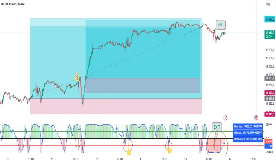
Power MarketPower Market Indicator
Description: The Power Market Indicator is designed to help traders assess market strength and make informed decisions for entering and exiting positions. This innovative indicator provides a comprehensive view of the evolution of Simple Moving Averages (SMA) over different periods and offers a clear measure of market strength through a total score.
Key Features:
Multi-Period SMA Analysis:
Calculates Simple Moving Averages (SMA) for 10 different periods ranging from 10 to 100.
Provides detailed analysis by comparing the current closing price with these SMAs.
Market Strength Measurement:
Assesses market strength by calculating a total score based on the relationship between the closing price and the SMAs.
The total score is displayed as a histogram with distinct colors for positive and negative values.
Smoothed Curve for Better View:
A smoothing of the total score is applied using a 5-period Simple Moving Average to represent the overall trend more smoothly.
Dynamic Information Table:
Real-time display of the maximum and minimum values among the SMAs, as well as the difference between these values, providing valuable insights into the variability of moving averages.
Visual Reference Lines:
Horizontal lines at zero, +50, and -50 for easy evaluation of key score levels.
How to Use the Indicator:
Position Entries: Use high positive scores to identify buying opportunities when market strength is strong.
Position Exits: Negative scores may signal market weakness, allowing you to exit positions or wait for a better opportunity.
Data Analysis: The table helps you understand the variability of SMAs, offering additional context for your trading decisions.
This powerful tool provides an in-depth view of market dynamics and helps you navigate your trading strategies with greater confidence. Embrace the Power Market Indicator and optimize your trading decisions today!
ADX & DI with dynamic threshold indicator
ADX and DI with Dynamic Threshold
This Pine Script indicator, "ADX & DI with Dynamic Threshold," helps traders detect trends, trend reversals, and trend strength using the Average Directional Index (ADX) and the Directional Indexes (DI+ and DI-). It incorporates a dynamic threshold calculated using the average ADX over a user-defined period, along with a fixed minimum threshold, making trend detection more flexible and adaptable.
ADX and Directional Indexes (DI+ and DI-)
ADX measures the strength of a trend, while DI+ and DI- measure the direction of the trend. High DI+ signals upward price strength, and high DI- signals downward price strength.
Dynamic Threshold
A threshold based on the average ADX over a certain number of periods, ensuring the indicator adapts to market conditions. The threshold is compared to DI+ and DI- to generate trend signals.
Fixed Minimum Threshold
A user-defined minimum threshold ensures that signals are only generated in markets with a certain level of trend strength, preventing false signals in low-trending markets.
Visual Highlights
The background color highlights:
Green for potential uptrend,
Red for potential downtrend, and
Orange when directional movement is strong but trend strength is weak, helping traders avoid false signals in sideways markets.
Customization
Several input parameters allow for complete customization of the indicator, ensuring it can adapt to different timeframes and assets.
How to Use
Length (len)
This is the smoothing period used to calculate the ADX and DI+/- values. Range: 5 to 50 (default: 14).
Threshold Period (th_period)
Determines the number of periods over which the dynamic ADX threshold is calculated. Range: 5 to 200 (default: 50).
Fixed Minimum Threshold (fixed_th)
The minimum ADX value that must be exceeded for the indicator to trigger signals. Range: 10 to 40 (default: 20).
Smoothing Method
Choose between SMA (Simple Moving Average) or EMA (Exponential Moving Average) for smoothing the true range and directional movement calculations.
DI+ (Green)
Indicates the strength of upward price movements.
DI- (Red)
Indicates the strength of downward price movements.
ADX (Navy)
Indicates the overall strength of the trend, regardless of direction.
Dynamic Threshold (Gray)
The dynamic threshold used for comparing ADX values.
Fixed Threshold Line
A dotted black line showing the user-defined minimum threshold for ADX.
Green Background
Indicates a potential uptrend when DI+ > DI- and ADX is above the threshold.
Red Background
Indicates a potential downtrend when DI- > DI+ and ADX is above the threshold.
Orange Background
Indicates that DI+ or DI- are strong, but ADX is weak, suggesting a lack of trend strength despite directional movement, which could lead to false signals.
Adjust the length (len) based on the volatility of the asset. A lower len (e.g., 10) may be suitable for faster timeframes (like 5-min charts), while a higher value (e.g., 20-30) may work better on longer timeframes.
Use the threshold period (th_period) to fine-tune the dynamic ADX threshold. A higher value smooths the dynamic threshold over a longer period, making it more resistant to sudden volatility.
Fixed Threshold (fixed_th) should be set based on the strength of trends you want to capture. A higher value (e.g., 30-40) is more conservative and will only trigger signals in very strong trends.
Example Usage
This indicator can be used to:
Identify trends: When the ADX crosses the threshold and DI+ or DI- is dominant, indicating an uptrend or downtrend.
Spot trend reversals: When DI+ and DI- cross each other with a strong ADX reading.
Avoid false signals: By recognizing when DI+ or DI- are strong, but the ADX is below the threshold (highlighted in orange).
Conclusion
The ADX and DI with Dynamic Threshold indicator is a versatile tool for trend-following strategies. It adapts to market conditions using dynamic and fixed thresholds and provides clear visual signals to help traders make informed decisions about market direction and trend strength.
By adjusting the various input parameters, this indicator can be tailored to any asset class or timeframe, making it suitable for all types of traders, from scalpers to swing traders.
Feel free to experiment with different settings and incorporate this indicator into your trading strategy for enhanced market analysis.

Larry Connors RSI 3 StrategyThe Larry Connors RSI 3 Strategy is a short-term mean-reversion trading strategy. It combines a moving average filter and a modified version of the Relative Strength Index (RSI) to identify potential buying opportunities in an uptrend. The strategy assumes that a short-term pullback within a long-term uptrend is an opportunity to buy at a discount before the trend resumes.
Components of the Strategy:
200-Day Simple Moving Average (SMA): The price must be above the 200-day SMA, indicating a long-term uptrend.
2-Period RSI: This is a very short-term RSI, used to measure the speed and magnitude of recent price changes. The standard RSI is typically calculated over 14 periods, but Connors uses just 2 periods to capture extreme overbought and oversold conditions.
Three-Day RSI Drop: The RSI must decline for three consecutive days, with the first drop occurring from an RSI reading above 60.
RSI Below 10: After the three-day drop, the RSI must reach a level below 10, indicating a highly oversold condition.
Buy Condition: All the above conditions must be satisfied to trigger a buy order.
Sell Condition: The strategy closes the position when the RSI rises above 70, signaling that the asset is overbought.
Who Was Larry Connors?
Larry Connors is a trader, author, and founder of Connors Research, a firm specializing in quantitative trading research. He is best known for developing strategies that focus on short-term market movements. Connors co-authored several popular books, including "Street Smarts: High Probability Short-Term Trading Strategies" with Linda Raschke, which has become a staple among traders seeking reliable, rule-based strategies. His research often emphasizes simplicity and robust testing, which appeals to both retail and institutional traders.
Scientific Foundations
The Relative Strength Index (RSI), originally developed by J. Welles Wilder in 1978, is a momentum oscillator that measures the speed and change of price movements. It oscillates between 0 and 100 and is typically used to identify overbought or oversold conditions in an asset. However, the use of a 2-period RSI in Connors' strategy is unconventional, as most traders rely on longer periods, such as 14. Connors' research showed that using a shorter period like 2 can better capture short-term reversals, particularly when combined with a longer-term trend filter such as the 200-day SMA.
Connors' strategies, including this one, are built on empirical research using historical data. For example, in a study of over 1,000 signals generated by this strategy, Connors found that it performed consistently well across various markets, especially when trading ETFs and large-cap stocks (Connors & Alvarez, 2009).
Risks and Considerations
While the Larry Connors RSI 3 Strategy is backed by empirical research, it is not without risks:
Mean-Reversion Assumption: The strategy is based on the premise that markets revert to the mean. However, in strong trending markets, the strategy may underperform as prices can remain oversold or overbought for extended periods.
Short-Term Nature: The strategy focuses on very short-term movements, which can result in frequent trading. High trading frequency can lead to increased transaction costs, which may erode profits.
Market Conditions: The strategy performs best in certain market environments, particularly in stable uptrends. In highly volatile or strongly trending markets, the strategy's performance can deteriorate.
Data and Backtesting Limitations: While backtests may show positive results, they rely on historical data and do not account for future market conditions, slippage, or liquidity issues.
Scientific literature suggests that while technical analysis strategies like this can be effective in certain market conditions, they are not foolproof. According to Lo et al. (2000), technical strategies may show patterns that are statistically significant, but these patterns often diminish once they are widely adopted by traders.
References
Connors, L., & Alvarez, C. (2009). Short-Term Trading Strategies That Work. TradingMarkets Publishing Group.
Lo, A. W., Mamaysky, H., & Wang, J. (2000). Foundations of Technical Analysis: Computational Algorithms, Statistical Inference, and Empirical Implementation. The Journal of Finance, 55(4), 1705-1770.
Wilder, J. W. (1978). New Concepts in Technical Trading Systems. Trend Research

Grid Bot Parabolic [xxattaxx]🟩 The Grid Bot Parabolic, a continuation of the Grid Bot Simulator Series , enhances traditional gridbot theory by employing a dynamic parabolic curve to visualize potential support and resistance levels. This adaptability is particularly useful in volatile or trending markets, enabling traders to explore grid-based strategies and gain deeper market insights. The grids are divided into customizable trade zones that trigger signals as prices move into new zones, empowering traders to gain deeper insights into market dynamics and potential turning points.
While traditional grid bots excel in ranging markets, the Grid Bot Parabolic’s introduction of acceleration and curvature adds new dimensions, enabling its use in trending markets as well. It can function as a traditional grid bot with horizontal lines, a tilted grid bot with linear slopes, or a fully parabolic grid with curves. This dynamic nature allows the indicator to adapt to various market conditions, providing traders with a versatile tool for visualizing dynamic support and resistance levels.
🔑 KEY FEATURES 🔑
Adaptable Grid Structures (Horizontal, Linear, Curved)
Buy and Sell Signals with Multiple Trigger/Confirmation Conditions
Secondary Buy and Secondary Sell Signals
Projected Grid Lines
Customizable Grid Spacing and Zones
Acceleration and Curvature Control
Sensitivity Adjustments
📐 GRID STRUCTURES 📐
Beyond its core parabolic functionality, the Parabolic Grid Bot offers a range of grid configurations to suit different market conditions and trading preferences. By adjusting the "Acceleration" and "Curvature" parameters, you can transform the grid's structure:
Parabolic Grids
Setting both acceleration and curvature to non-zero values results in a parabolic grid.This configuration can be particularly useful for visualizing potential turning points and trend reversals. Example: Accel = 10, Curve = -10)
Linear Grids
With a non-zero acceleration and zero curvature, the grid tilts to represent a linear trend, aiding in identifying potential support and resistance levels during trending phases. Example: Accel =1.75, Curve = 0
Horizontal Grids
When both acceleration and curvature are set to zero, the indicator reverts to a traditional grid bot with horizontal lines, suitable for ranging markets. Example: Accel=0, Curve=0
⚙️ INITIAL SETUP ⚙️
1.Adding the Indicator to Your Chart
Locate a Starting Point: To begin, visually identify a price point on your chart where you want the grid to start.This point will anchor your grid.
2. Setting Up the Grid
Add the Grid Bot Parabolic Indicator to your chart. A “Start Time/Price” dialog will appear
CLICK on the chart at your chosen start point. This will anchor the start point and open a "Confirm Inputs" dialog box.
3. Configure Settings. In the dialog box, you can set the following:
Acceleration: Adjust how quickly the grid reacts to price changes.
Curve: Define the shape of the parabola.
Intervals: Determine the distance between grid levels.
If you choose to keep the default settings, with acceleration set to 0 and curve set to 0, the grid will display as traditional horizontal lines. The grid will align with your selected price point, and you can adjust the settings at any time through the indicator’s settings panel.
⚙️ CONFIGURATION AND SETTINGS ⚙️
Grid Settings
Accel (Acceleration): Controls how quickly the price reacts to changes over time.
Curve (Curvature): Defines the overall shape of the parabola.
Intervals (Grid Spacing): Determines the vertical spacing between the grid lines.
Sensitivity: Fine tunes the magnitude of Acceleration and Curve.
Buy Zones & Sell Zones: Define the number of grid levels used for potential buy and sell signals.
* Each zone is represented on the chart with different colors:
* Green: Buy Zones
* Red: Sell Zones
* Yellow: Overlap (Buy and Sell Zones intersect)
* Gray: Neutral areas
Trigger: Chooses which part of the candlestick is used to trigger a signal.
* `Wick`: Uses the high or low of the candlestick
* `Close`: Uses the closing price of the candlestick
* `Midpoint`: Uses the middle point between the high and low of the candlestick
* `SWMA`: Uses the Symmetrical Weighted Moving Average
Confirm: Specifies how a signal is confirmed.
* `Reverse`: The signal is confirmed if the price moves in the opposite direction of the initial trigger
* `Touch`: The signal is confirmed when the price touches the specified level or zone
Sentiment: Determines the market sentiment, which can influence signal generation.
* `Slope`: Sentiment is based on the direction of the curve, reflecting the current trend
* `Long`: Sentiment is bullish, favoring buy signals
* `Short`: Sentiment is bearish, favoring sell signals
* `Neutral`: Sentiment is neutral. No secondary signals will be generated
Show Signals: Toggles the display of buy and sell signals on the chart
Chart Settings
Grid Colors: These colors define the visual appearance of the grid lines
Projected: These colors define the visual appearance of the projected lines
Parabola/SWMA: Adjust colors as needed. These are disabled by default.
Time/Price
Start Time & Start Price: These set the starting point for the parabolic curve.
* These fields are automatically populated when you add the indicator to the chart and click on an initial location
* These can be adjusted manually in the settings panel, but he easiest way to change these is by directly interacting with the start point on the chart
Please note: Time and Price must be adjusted for each chart when switching assets. For example, a Start Price on BTCUSD of $60,000 will not work on an ETHUSD chart.
🤖 ALGORITHM AND CALCULATION 🤖
The Parabolic Function
At the core of the Parabolic Grid Bot lies the parabolic function, which calculates a dynamic curve that adapts to price action over time. This curve serves as the foundation for visualizing potential support and resistance levels.
The shape and behavior of the parabola are influenced by three key user-defined parameters:
Acceleration: This parameter controls the rate of change of the curve's slope, influencing its tilt or steepness. A higher acceleration value results in a more pronounced tilt, while a lower value leads to a gentler slope. This applies to both curved and linear grid configurations.
Curvature: This parameter introduces and controls the curvature or bend of the grid. A higher curvature value results in a more pronounced parabolic shape, while a lower value leads to a flatter curve or even a straight line (when set to zero).
Sensitivity: This setting fine-tunes the overall responsiveness of the grid, influencing how strongly the Acceleration and Curvature parameters affect its shape. Increasing sensitivity amplifies the impact of these parameters, making the grid more adaptable to price changes but potentially leading to more frequent adjustments. Decreasing sensitivity reduces their impact, resulting in a more stable grid structure with fewer adjustments. It may be necessary to adjust Sensitivity when switching between different assets or timeframes to ensure optimal scaling and responsiveness.
The parabolic function combines these parameters to generate a curve that visually represents the potential path of price movement. By understanding how these inputs influence the parabola's shape and behavior, traders can gain valuable insights into potential support and resistance areas, aiding in their decision-making process.
Sentiment
The Parabolic Grid Bot incorporates sentiment to enhance signal generation. The "Sentiment" input allows you to either:
Manually specify the market sentiment: Choose between 'Long' (bullish), 'Short' (bearish), or 'Neutral'.
Let the script determine sentiment based on the slope of the parabolic curve: If 'Slope' is selected, the sentiment will be considered 'Long' when the curve is sloping upwards, 'Short' when it's sloping downwards, and 'Neutral' when it's flat.
Buy and Sell Signals
The Parabolic Grid Bot generates buy and sell signals based on the interaction between the price and the grid levels.
Trigger: The "Trigger" input determines which part of the candlestick is used to trigger a signal (wick, close, midpoint, or SWMA).
Confirmation: The "Confirm" input specifies how a signal is confirmed ('Reverse' or 'Touch').
Zones: The number of "Buy Zones" and "Sell Zones" determines the areas on the grid where buy and sell signals can be generated.
When the trigger condition is met within a buy zone and the confirmation criteria are satisfied, a buy signal is generated. Similarly, a sell signal is generated when the trigger and confirmation occur within a sell zone.
Secondary Signals
Secondary signals are generated when a regular buy or sell signal contradicts the prevailing sentiment. For example:
A buy signal in a bearish market (Sentiment = 'Short') would be considered a "secondary buy" signal.
A sell signal in a bullish market (Sentiment = 'Long') would be considered a "secondary sell" signal.
These secondary signals are visually represented on the chart using hollow triangles, differentiating them from regular signals (filled triangles).
While they can be interpreted as potential contrarian trade opportunities, secondary signals can also serve other purposes within a grid trading strategy:
Exit Signals: A secondary signal can suggest a potential shift in market sentiment or a weakening trend. This could be a cue to consider exiting an existing position, even if it's currently profitable, to lock in gains before a potential reversal
Risk Management: In a strong trend, secondary signals might offer opportunities for cautious counter-trend trades with controlled risk. These trades could utilize smaller position sizes or tighter stop-losses to manage potential downside if the main trend continues
Dollar-Cost Averaging (DCA): During a prolonged trend, the parabolic curve might generate multiple secondary signals in the opposite direction. These signals could be used to implement a DCA strategy, gradually accumulating a position at potentially favorable prices as the market retraces or consolidates within the larger trend
Secondary signals should be interpreted with caution and considered in conjunction with other technical indicators and market context. They provide additional insights into potential market reversals or consolidation phases within a broader trend, aiding in adapting your grid trading strategy to the evolving market dynamics.
Examples
Trigger=Wick, Confirm=Touch. Signals are generated when the wick touches the next gridline.
Trigger=Close, Confirm=Touch. Signals require the close to touch the next gridline.
Trigger=SWMA, Confirm=Reverse. Signals are triggered when the Symmetrically Weighted Moving Average reverse crosses the next gridline.
🧠THEORY AND RATIONALE 🧠
The innovative approach of the Parabolic Grid Bot can be better understood by first examining the limitations of traditional grid trading strategies and exploring how this indicator addresses them by incorporating principles of market cycles and dynamic price behavior
Traditional Grid Bots: One-Dimensional and Static
Traditional grid bots operate on a simple premise: they divide the price chart into a series of equally spaced horizontal lines, creating a grid of trading zones. These bots excel in ranging markets where prices oscillate within a defined range. Buy and sell orders are placed at these grid levels, aiming to profit from mean reversion as prices bounce between the support and resistance zones.
However, traditional grid bots face challenges in trending markets. As the market moves in one direction, the bot continues to place orders in that direction, leading to a stacking of positions. If the market eventually reverses, these stacked trades can be profitable, amplifying gains. But the risk lies in the potential for the market to continue trending, leaving the trader with a series of losing trades on the wrong side of the market
The Parabolic Grid Bot: Adding Dimensions
The Parabolic Grid Bot addresses the limitations of traditional grid bots by introducing two additional dimensions:
Acceleration (Second Dimension): This parameter introduces a second dimension to the grid, allowing it to tilt upwards or downwards to align with the prevailing market trend. A positive acceleration creates an upward-sloping grid, suitable for uptrends, while a negative acceleration results in a downward-sloping grid, ideal for downtrends. The magnitude of acceleration controls the steepness of the tilt, enabling you to fine-tune the grid's responsiveness to the trend's strength
Curvature (Third Dimension): This parameter adds a third dimension to the grid by introducing a parabolic curve. The curve's shape, ranging from gentle bends to sharp turns, is controlled by the curvature value. This flexibility allows the grid to closely mirror the market's evolving structure, potentially identifying turning points and trend reversals.
Mean Reversion in Trending Markets
Even in trending markets, the Parabolic Grid Bot can help identify opportunities for mean reversion strategies. While the grid may be tilted to reflect the trend, the buy and sell zones can capture short-term price oscillations or consolidations within the broader trend. This allows traders to potentially pinpoint entry and exit points based on temporary pullbacks or reversals.
Visualize and Adapt
The Parabolic Grid Bot acts as a visual aid, enhancing your understanding of market dynamics. It allows you to "see the curve" by adapting the grid to the market's patterns. If the market shows a parabolic shape, like an upward curve followed by a peak and a downward turn (similar to a head and shoulders pattern), adjust the Accel and Curve to match. This highlights potential areas of interest for further analysis.
Beyond Straight Lines: Visualizing Market Cycle
Traditional technical analysis often employs straight lines, such as trend lines and support/resistance levels, to interpret market movements. However, many analysts, including Brian Millard, contend that these lines can be misleading. They propose that what might appear as a straight line could represent just a small part of a larger curve or cycle that's not fully visible on the chart.
Markets are inherently cyclical, marked by phases of expansion, contraction, and reversal. The Parabolic Grid Bot acknowledges this cyclical behavior by offering a dynamic, curved grid that adapts to these shifts. This approach helps traders move beyond the limitations of straight lines and visualize potential support and resistance levels in a way that better reflects the market's true nature
By capturing these cyclical patterns, whether subtle or pronounced, the Parabolic Grid Bot offers a nuanced understanding of market dynamics, potentially leading to more accurate interpretations of price action and informed trading decisions.
⚠️ DISCLAIMER⚠️
This indicator utilizes a parabolic curve fitting approach to visualize potential support and resistance levels. The mathematical formulas employed have been designed with adaptability and scalability in mind, aiming to accommodate various assets and price ranges. While the resulting curves may visually resemble parabolas, it's important to note that they might not strictly adhere to the precise mathematical definition of a parabola.
The indicator's calculations have been tested and generally produce reliable results. However, no guarantees are made regarding their absolute mathematical accuracy. Traders are encouraged to use this tool as part of their broader analysis and decision-making process, combining it with other technical indicators and market context.
Please remember that trading involves inherent risks, and past performance is not indicative of future results. It is always advisable to conduct your own research and exercise prudent risk management before making any trading decisions.
🧠 BEYOND THE CODE 🧠
The Parabolic Grid Bot, like the other grid bots in this series, is designed with education and community collaboration in mind. Its open-source nature encourages exploration, experimentation, and the development of new grid trading strategies. We hope this indicator serves as a framework and a starting point for future innovations in the field of grid trading.
Your comments, suggestions, and discussions are invaluable in shaping the future of this project. We welcome your feedback and look forward to seeing how you utilize and enhance the Parabolic Grid Bot.

QQQ and SPY Price Levels [MW]Introduction:
Don’t let SPY and QQQ resistance levels hurt your futures trading anymore. The QQQ and SPY Price Levels indicator automagically provides easily accessible QQQ price levels for NASDAQ-related charts such as QQQ, /NQ and /MNQ futures, and leveraged ETFs such as TQQQ and SQQQ as well as for SPY price levels for S&P 500-related charts such as SPY, /ES and /MES futures, SPX, and leveraged ETFs such as UPRO and SPXU. If you’ve ever traded futures, or anything QQQ- or SPY-related and wanted to know at what price would the corresponding asset reach a key whole number level of QQQ or SPY, like 400, 440, 445, or even 447.50, this tool is for you. Key 10x, 5x, and even 2.5x multiples of QQQ and SPY can act as support or resistance for other related-assets. Until now, there hasn’t been an indicator that can serve as an easy visual cue to know exactly when that is about to happen across assets.
This indicator is a fork of the original SPY Price Levels indicator, which only considered SPY-related assets.
Settings:
QQQ/SPY 2.5x: Show closest levels above and below that are multiples of 2.5 on QQQ
QQQ/SPY 5x: Show closest levels above and below that are multiples of 5 on QQQ
QQQ/SPY 10x: Show closest levels above and below that are multiples of 10 on QQQ
Show QQQ/SPY Price Label: Show the current QQQ/SPY price
Extend lines to the left: Extend label lines for each price level to the beginning of the chart
Calculations:
This indicator defines the ratio between the price of QQQ/SPY and another NASDAQ/S&P-related asset and uses that multiplier once the user-defined price increments are defined. For example, if /MNQ is at 19000 and QQQ is at 465, then the ratio would be 40.8.
The incremental QQQ levels that are above and below the QQQ price are calculated using the following equations:
qqqLevelUp = _multiplier * math.ceil(_qqqClose / _multiplier)
qqqLevelDown = _multiplier * math.floor(_qqqClose / _multiplier)
The conversion ratio is then multiplied by that amount to get the final estimated corresponding price using the calculation:
levelUp := _conversion * qqqLevelUp
levelDown := _conversion * qqqLevelDown
For leveraged assets, the conversion must be used on the difference between the current QQQ price and the incremental upper and lower levels.
For example, the calculation for the next level up looks like the following:
levelUpDelta := math.abs(_qqqClose - qqqLevelUp)
levelUp := close + _conversion * (levelUpDelta * _leverage)
This logic is identical for SPY-related assets.
How to Use:
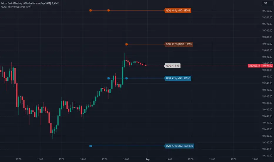
The QQQ and SPY Price Levels indicator aims to be as unobtrusive as possible. The default view shows 3 labels and 2 lines that are all aligned to the right of the main chart, so that it interferes as little as possible with any other indicators. It can be added to any /NQ or /MNQ futures chart, SQQQ, TQQQ, and, of course, QQQ as well as any /ES /MES futures chart, SPXU, UPRO, SPX, and of course SPY. The most immediate price levels for each multiplier appears above and below the current price along with the price of QQQ/SPY.
For example, MNQU2024 is currently at 19594. By looking at the indicator the next QQQ increment below is at 475, or 19556 on the MNQU2024 chart. This potential support is marked with a green label that shows both prices. The next increment above is at QQQ 477.50, or 19659 on the MESU2024 chart. And the QQQ price itself, is also shown (and can be removed) at 475.92.
QQQ and SPY price increments of 2.5, 5, and 10 tend to consistently act at the very least as emotional support and resistance levels. Weak, or weakening volume and/or momentum when these levels are hit can trigger a strong rejection, and can sometimes precipitate lengthy consolidation periods at those levels. Watching an NASDAQ- and S&P 500-related asset come to a halt, fall off a cliff, or react in some other unintuitive way could very well be the result of a QQQ/SPY level being reached. Even though many of us know that this relationship exists, it’s easy to forget. So, this indicator helps to ensure that its users keep that relationship front and center.
By extending the lines into the past on QQQ/SPY and their related assets, you can see what reactions happened at these key levels.
Other Usage Notes and Limitations:
The calculations used only provide an estimated relationship or a close approximation, and are not exact.
It's important for traders to be aware of the limitations of any indicator and to use them as part of a broader, well-rounded trading strategy that includes risk management, fundamental analysis, and other tools that can help with reducing false signals, determining trend direction, and providing additional confirmation for a trade decision. Diversifying strategies and not relying solely on one type of indicator or analysis can help mitigate some of these risks.
Yield Curve InversionThe Yield Curve Inversion indicator is a tool designed to help traders and analysts visualize and interpret the dynamics between the US 10-year and 2-year Treasury yields. This indicator is particularly useful for identifying yield curve inversions, often seen as a precursor to economic recessions.
Features and Interpretations
Display Modes: Choose between "Spread Mode" to visualize the yield spread indicating normal (green) or inverted (red) curves, or "Both Yields Mode" to view both yields.
Yield Spread: A plotted difference between 10-year and 2-year yields, with a zero line marking inversion. A negative spread suggests potential economic downturns.
Color Coding: Green for a normal yield curve (10Y > 2Y) and red for an inverted curve (2Y > 10Y).
Legend: Provides quick reference to yield curve states for easier interpretation.
This indicator is for educational and informational purposes only. It should not be considered financial advice or a recommendation to buy or sell any financial instruments. Users should conduct their own research and consult with a financial advisor before making investment decisions. The creator of this indicator is not responsible for any financial losses incurred through its use.

Super RSI: Multi-Timeframe, Multi-RSI-MA, Multi Symbol [DucTri]█ Overview
RSI is a very popular indicator that almost every trader knows about. I created this indicator with the goal of helping you use RSI more conveniently and effectively.
█ Uses
Monitor the RSI of 10 currency pairs simultaneously.
The first column shows the RSI of the current currency pair.
RSI below 30 will have a Red background, and above 70 will have a Green background.
Display multiple RSI lines with different lengths (or timeframes).
Displays 3 RSI with 3 different lengths 7, 14 and 21
Displays two RSI lines with two different timeframes. The purple line shows RSI (14) for the 1H timeframe, and the blue line shows RSI (14) for the 4H timeframe.
Display MA and Bollinger Band lines for RSI.
Shows the RSI line along with two MA lines of the RSI: EMA (9) in blue and WMA (45) in red.
Identify RSI Divergence with custom settings
█ Input
- You can have up to three RSI lines, with customizable lengths and timeframes.
- You also have up to three RSI-MA lines, where you can customize the MA type and length.
- You can track RSI for up to 10 currency pairs at the same time.
- Additionally, you can change how the top (or bottom) is determined when identifying divergence.
█ Alerts
Send alerts when two RSI lines cross. For example, when the RSI 14 crosses above the RSI 21, or the RSI on the 1H timeframe crosses above the RSI on the 4H timeframe.*
Send alerts when RSI crosses above or below the RSI-MA line.
Send alerts when two RSI-MA lines cross. For example, when the RSI-EMA (9) crosses above the RSI-WMA (45).*
Send alerts when Divergence (Convergence) appears.
Send alerts when any currency pair in the monitored list shows an Overbought or Oversold signal.

Inverted Yield Curve (US01Y/US10Y Ratio)This indicator calculates and visualizes the ratio between the US 1-Year Treasury Yield (US01Y) and the US 10-Year Treasury Yield (US10Y). It provides a clear visual representation of the relationship between short-term and long-term interest rates, which can be a valuable tool for analyzing market conditions, potential recessions, or shifts in economic outlook.
Features:
US01Y/US10Y Ratio: The indicator plots the ratio between the 1-Year and 10-Year US Treasury Yields as a smooth curve.
Dynamic Highlighting: Portions of the curve where the ratio exceeds 1 are highlighted in red, making it easy to identify periods where short-term rates surpass long-term rates—a key signal often associated with economic shifts or inversions.
Customizable Appearance: The main curve is plotted in a light blue color for clear visibility against most chart backgrounds.
Use Cases:
Yield Curve Analysis: This indicator helps traders and analysts monitor the yield curve, specifically focusing on the relationship between short-term and long-term interest rates.
Recession Signals: An inverted yield curve, where the ratio exceeds 1, can be an early warning signal for potential economic downturns.
Market Sentiment: Use the indicator to gauge shifts in investor sentiment by tracking changes in the yield curve over time.
How to Use:
Add the script to your TradingView chart.
The light blue curve represents the ratio of US01Y/US10Y.
Red highlights indicate periods where the ratio exceeds 1, signaling potential yield curve inversion.
This indicator is ideal for traders, investors, and economists looking to incorporate yield curve analysis into their trading strategies or economic forecasts.

Daily Levels Percentual [TOLK] Settings Crypto and ForexPercentage zones refer to specific areas or bands on the price chart of a financial asset that are bounded by percentages of change relative to a reference point, such as the opening price or a reference value from a previous move.
These zones are useful for identifying support and resistance levels, predicting possible price reversals, or setting price targets. For example, on a price chart, you can create percentage zones to observe how the price behaves when it reaches 1%, 2%, 5%, 10%, etc., above or below a certain point.
These zones can be used in conjunction with other technical analysis tools, such as Fibonacci, moving averages, or volume analysis, to improve decision-making in trading strategies.
The default indicator levels are as follows:
SETTINGS Crypto:
Crypto Level 1 > 1.0%
Crypto Level 2 > 1.618%
Crypto Level 3 > 2.0%
Crypto Level 4 > 2.618%
Crypto Level 5 > 3.618%
Crypto Level 6 > 4.618%
Crypto Level 7 > 5.0%
Crypto Level 8 > 7.618%
Crypto Level 9 > 10.0%
Crypto Level 10 > 12.618%
Crypto Level 11 > 13.618%
Crypto Level 12 > 15%
Crypto Level 13 > 17.618%
Crypto Level 14 > 20%
SETTINGS Forex:
Forex Level 1 > 0.10%
Forex Level 2 > 0.1618%
Forex Level 3 > 0.20%
Forex Level 4 > 0.2618%
Forex Level 5 > 0.3618%
Forex Level 6 > 0.4618%
Forex Level 7 > 0.50%
Forex Level 8 > 0.7618%
Forex Level 9 > 1.0%
Forex Level 10 > 1.2618%
Forex Level 11 > 1.3618%
Forex Level 12 > 1.50%
Forex Level 13 > 1.7618%
Forex Level 14 > 2.0%
Percentage Levels This approach helps identify critical price levels where the asset may encounter support or resistance, making it easier to make trading decisions based on price movement patterns.

Wedge Pop & Drop [QuantVue]A "Wedge Pop" is a trading pattern popularized by Oliver Kell, a notable trader who won the 2020 US Investing Championship with a remarkable return of 941%. This pattern, often referred to as "The Money Pattern" in his trading strategy, serves as a critical signal indicating the beginning of a new uptrend in a stock.
A Wedge Pop occurs when a stock first trades up through the moving averages after reaching a downside extension. Conversely, a Wedge Drop refers to the first time a stock trades down through the moving averages after reaching an upside extension.
How the Indicator Works:
The indicator uses the Average True Range (ATR) and the 10-period Exponential Moving Average (10 EMA) to identify upside and downside extensions. An upside extension occurs when the low of the current bar is greater than 1.5 (default) times the ATR above the moving average. A downside extension occurs when the high of the current bar is less than 1.5 times the ATR below the moving average.
Once an extension has been reached, the first time the security trades back through the moving averages, it triggers a Wedge Pop/Drop.
Give this indicator a BOOST and COMMENT your thoughts below!
We hope you enjoy.
Cheers!

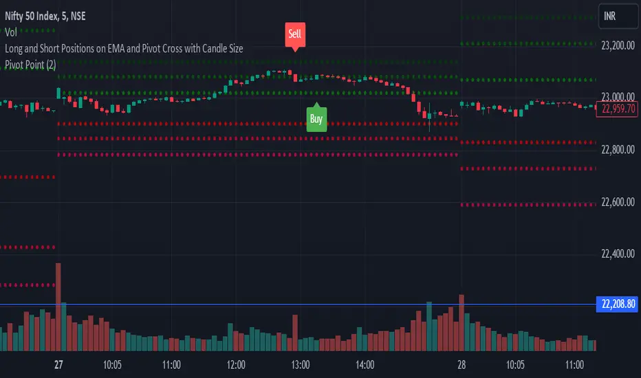
Long and Short Positions on EMA and Pivot Cross with Candle Size
This Pine Script indicator identifies long and short trading signals based on specific criteria involving candle body size, EMA, and pivot levels.
Long Position ("Buy" Signal): A "Buy" signal is triggered when a green candle (close > open) with a body size of at least 10 crosses above the 9 EMA and any of the daily pivot levels (R1, R2, R3, R4, R5, S1, S2, S3, S4, S5).
Short Position ("Sell" Signal): A "Sell" signal is triggered when a red candle (close < open) with a body size of at least 10 crosses below the 9 EMA and any of the pivot levels.
The script plots only the "Buy" and "Sell" signals on the chart, without displaying the EMA or pivot levels.
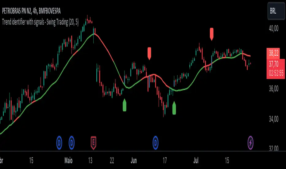
Trend identifier with signals - Swing TradingIndicator Objective
The "Trend identifier with signals - Swing Trading" indicator is designed to help traders identify market trends and provide clear visual signals for potential buy and sell points based on the interaction of price with the 20-period moving average.
How the Indicator Works
20-Period Moving Average:
The indicator calculates the 20-period simple moving average (SMA), which is a common tool for smoothing out price fluctuations and identifying the overall market direction.
The moving average is plotted on the chart, changing color according to the identified trend:
Green: Indicates an uptrend.
Red: Indicates a downtrend.
Gray: Indicates a neutral or undefined market condition.
Trend Identification on the Daily Chart:
The indicator checks the trend based on an adjustable period (default is 5 periods):
Uptrend: When the short-term moving average (5 periods) is above the long-term moving average (10 periods).
Downtrend: When the short-term moving average (5 periods) is below the long-term moving average (10 periods).
Signal for Touching the Moving Average:
When the price crosses the 20-period moving average, the candles are colored purple to indicate that there was a touch on the moving average.
This helps identify critical points where the price may reverse or continue its trend.
Trend Signal:
Green Flag: Appears below the candle when there is a touch on the moving average and the trend is up, suggesting a potential buy point.
Red Flag: Appears above the candle when there is a touch on the moving average and the trend is down, suggesting a potential sell point.
Lateral Zone Identification:
The indicator also checks if the price touched the moving average for 5 consecutive candles, indicating a possible consolidation or lateral zone.
If this occurs, a message "Possible Lateral Zone" is shown on the chart, helping the trader avoid trades in a market without a clear direction.
How the Indicator Helps Traders
Clear Trend Identification:
By changing the color of the moving average according to the trend (green for up, red for down), the indicator provides a clear visualization of market direction.
This allows traders to align their trades with the prevailing trend, increasing the probability of success.
Visual Buy and Sell Signals:
The green and red flags provide direct visual signals for potential entry and exit points, based on the interaction of price with the moving average.
This is particularly useful for novice traders who may struggle to identify these points on their own.
Risk Management and Trade Planning:
Identifying lateral zones helps traders avoid trading in trendless markets, where price movements are more unpredictable.
This improves risk management and allows traders to focus on more favorable opportunities.
[SGM Return Distribution]Code Description
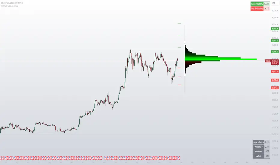
This Pine Script™ is designed to analyze the distribution of historical returns of a financial asset and project future confidence levels. It uses statistical techniques to estimate the probability of winning and losing as well as displaying confidence bands and distribution statistics.
User Entries
Length (252): The number of days used to calculate statistics.
Offset (20): Offset used to project future values.
Projection Days (10): Number of days projected into the future.
Smoothing Confidence Levels (10): Smoothing confidence bands.
Display Settings
Plot Distribution: Shows the distribution of returns.
Show Probabilities: Shows winning and losing probabilities.
Show Distribution Stats: Shows distribution statistics.
Show Confidence Bands: Shows confidence bands.
Show Confidence Lines: Shows confidence lines.
Calculations and Features
Distribution of Yields:
Calculates logarithmic returns and their statistics (average, volatility, skewness, kurtosis).
Projects the average and volatility over the projected number of days.
Displays the distribution of returns as a histogram.
Confidence Interval:
Uses the inv_norm function to calculate Z scores for different confidence levels.
Calculates the upper and lower bounds of the confidence bands.
Probability Display:
Calculates and displays win and loss probabilities based on the distribution of returns.
Statistics Display:
Shows key statistics such as mean, volatility, skewness and kurtosis.
Trust Bands and Lines:
Shows confidence bands and lines based on calculated confidence levels.
Mathematical Assumptions Used
Logarithmic Returns: Returns are calculated using the logarithm of prices, which is common for financial time series because it makes returns independent of price level.
Normal Distribution for Confidence Bands: Confidence interval calculations are based on the assumption that returns follow a normal distribution.
Average and Volatility Projection: Average returns and volatility are projected over a future period assuming they remain constant.
Skewness and Kurtosis: Although these measures are calculated for understanding the distribution of returns, they are not used in box projections but can provide additional information about the distribution of historical returns.
Use in Trading
Risk Estimation: Confidence bands can help estimate likely future price levels, which is crucial for determining strike levels and risk management.
Risk Management: Use confidence bands to set stop-loss and take-profit levels.
Probability Analysis: Win and loss probabilities can help assess a position's likelihood of success.
Potential Problems
Assumption of Normality for Confidence Bands: Financial returns do not always follow a normal distribution, especially in the presence of extreme events (fat tails).
Stationarity: Assuming that return statistics (average, volatility) remain constant over time can be erroneous in volatile market periods.
Limited Historical Data: Using a limited history (252 days) may not capture all possible behaviors of the asset.
Input Parameters: Results can be sensitive to the input parameters chosen (length, offset, etc.).
Percentages from 52 Week HighThis script is helpful for anyone that wants to monitor 5, 10, 20, 30, 40, 50% drops from the 52 week moving high.
I have been using a version of this script for a few years now and thought I would share it back with the community as I wrote it in 2021 to find quick deals when flipping through charts of stocks I've been watching. I never seemed to find anything doing this simple yet intuitive thing and I found myself regularly computing these lines manually on each chart. This will save you from having to do that as it automatically draws each level on your chart based on the recent 52 week or daily high.
I recently added the ability to turn on/off different levels and defaulted to setting 5, 10, and 20 % drops from the 52 week high. You can also change this to be a 52 day moving high if that's your preference.
Please let me know if you have ideas for modification as I wanted to share this with the community given I had not seen anything out there giving me what I wanted - which is why I wrote it.
All the best friends.

T3 [RATE OF CHANGE] by SKiNNiEHDeveloped by Tim Tillson, the Tilson Moving Average (T3) is a trend indicator with the advantage of having less lag than other ones. That is, a faster moving average. The T3 moving average is an "indicator of an indicator" as it includes several EMAs of another EMA. Unlike other moving averages, the t3 adds the so-called volume factor, a value between 0 and 1.
The T3 RATE OF CHANGE by SKiNNiEH is a unique indicator that integrates the T3 moving average with a normalized Rate of Change (RoC) calculation. Unlike traditional T3 moving averages, this indicator provides additional smoothing modes (SINGLE, DOUBLE & TRIPLE) for the T3, whilst enhancing visual feedback of the plotted line by generating a dynamic line thickness, a dynamic line color & brightness and trade entry bars, offering traders a more dynamic view of market conditions without going "overboard" with settings.
How It Works
Visualization
The T3 line varies in thickness and color based on the RoC values, giving traders visual cues about market strength and direction.
Thicker and brighter lines indicate stronger trends, while thinner and duller lines suggest weaker trends.
Rate of Change Filte r
This filter refines trend detection by using the line thickness measurement.
Adjustable from 0 (disabled) to 4, where higher settings only consider stronger trends for signals.
The T3 line turns gray when the filter is triggered or when the RoC is extremely low, signaling a weak or neutral market.
T3 Calculation (mode)
SINGLE
The T3 calculation is applied once to the closing price.
This mode has the least smoothing effect and the least lag. It reacts more quickly to price changes but is less smooth.
DOUBLE
The T3 calculation is applied twice sequentially.
The first T3 calculation smooths the closing price.
The second T3 calculation smooths the result of the first T3 calculation.
This mode provides more smoothing and introduces more lag compared to SINGLE mode. It is smoother but reacts slower to price changes.
TRIPLE
The T3 calculation is applied three times sequentially.
The first T3 calculation smooths the closing price.
The second T3 calculation smooths the result of the first T3 calculation.
The third T3 calculation smooths the result of the second T3 calculation.
This mode provides the most smoothing and introduces the most lag by reacting the slowest to price changes.
Rate of Change (RoC) Calculation
The script calculates the Rate of Change (RoC) for the T3 values based on the selected mode (SINGLE, DOUBLE, TRIPLE). The RoC measures the percentage change between the most recent value and a value in the past. The measurement is then normalized in three different ranges.
Normalization 5: Determines T3 line thickness on a scale from 0 - 5
Normalization 10: Determines T3 color brightness on a scale from 0 - 10
Normalization 100: Determines Rate of Change percentage
Rate of Change Filter
The script uses the RoC filter to refine the trend detection logic. By using the line thickness measurement, a filter can be enabled by setting this input on 1 - 4. As an example, setting this to 4 means that only a line thickness of 5 would be considered for a trade signal. Setting this to 0 disables the filter. The T3 line will turn gray when the filter is triggered, the T3 line can also turn gray without the filter, when the Rate of Change is extremely low.
Trade Signals
A trade signal is printed as a vertical green or red bar when the following conditions are met:
Long:
Closing price is above the T3 line
Rate of Change percentage is above 0
Previous trade signal was a short signal **
Rate of Change is not filtered
Short:
Closing price is below the T3 line
Rate of Change percentage is below 0
Previous trade signal was a long signal **
Rate of Change is not filtered
** Or this is the very first recorded trade signal
It should be noted that the trade signals in this script are trade entry signals, not trade exit signals. Use at your own risk.
Instructions for Use
Setting Up the Indicator
Apply the indicator to your trading chart.
Choose the desired T3 mode (SINGLE, DOUBLE, TRIPLE) based on your need for smoothing and lag.
Set the desired length (lookback period).
Set the desired factor between 0 and 1 (increments of 0.1)
Choose an overall line thickness and brightness that suits your screen and taste preferences.
Apply the Rate of Change filter. Setting this to 0 will disable the filter
Tip: use the trade entry vertical bars as a visual calibration tool the adjust mode, length, factor and filter.
Interpreting Visual Cues
Observe the T3 line's thickness: thicker lines indicate stronger trends, while thinner lines suggest weaker trends.
Observe the T3 line's color and color brightness: green indicates a more bullish trend, while red indicates a more bearish trend. A brighter color suggest a stronger trend. A gray color means the RoC is very low / neutral, or the RoC filter is active.
Observe the T3 line's location relative to price: below price indicates a more bullish trend, above price indicates a more bearish trend. The T3 line distance from price can also be an indication of trend strength.
Observe vertical bars: a vertical bar is printed green when long conditions are met, a vertical bar is printed red when short conditions are met. See the rules that explain the trigger for this bar above.
Alerts
Go to the settings tab, set the condition to T3.RoC.S + LONG or SHORT.
Enter an alert name and message.
Configure your notification preferences in the notifications tab and create the alert
Notifications-tab: Choose your notification preferences
Create the alert.

Liquidity Swings & SweepsThis Pine script indicator is designed to create a visual representation liquidity as identified by swing Highs/Lows along with an indication of the liquidity level that was swept, optionally rating the strength of the sweep based on time & price.
Relevance:
Liquidity levels & sweeps are crucial for many SMC/ICT setups and can indicate a point at which the price changes direction or may re-trace in an opposite direction to provide additional liquidity for continued move in the original direction. Additionally, liquidity levels may provide targets for setups, as price action will often seek to take out those levels as they main contain many buy/sell stops.
How It Works:
The indicator tracks all swing points, as identified using user-defined strength of the swing. Once a swing is formed that meets the criteria, it is represented by a horizontal line starting at the price of the current swing until the last bar on the chart. While the swing is valid, this line will continue to be extended until the swing is invalid or a new swing is formed. Upon identifying a new swing, the indicator then scans the earlier swings in the same direction looking for a point of greatest liquidity that was taken by the current swing. This level is then denoted by dashed horizontal line, connecting earlier swing point to the current. At the same time any liquidity zones between the two swings are automatically removed from the chart if they had previously been rendered on the chart. If the setting to enable scan for maximum liquidity is enabled, then while looking back, the indicator will look for lowest low or highest high that was taken by the current swing point, which may not be a swing itself, however, is a lowest/highest price point taken (mitigated) by the current swing, which in many cases will be better price then then the one represented by previous swing. If the option to render sweep label is enabled, the sweep line will also be completed by a label, that will score the sweep and a tooltip showing the details of the level swept and the time it took to sweep it. The score explained further in configurability section ranks the strength of the sweep based on time and is complemented by price (difference in price between the two liquidity levels).
Configurability:
A user may configure the strength of the swing using both left/right strength (number of bars) as well as optionally instruct the indicator to seek the lowest/highest price point which may not be previous swing that was taken out by newly formed swing.
From appearance perspective liquidity level colors & line width presenting the liquidity/swing can be configured. There is also an option to render the liquidity sweep label that will generate an icon-based rating of the liquidity sweep and a tooltip that provides details on the scope of the swing, which includes liquidity level swept and when it was formed along with the time it took to sweep the liquidity.
Rating is of sweeps is primarily based on time with a secondary reference to price
💥- Best rating, very strong sweep with an hourly or better liquidity sweep
🔥- Second rating, strong sweep with 15 – 59 minute liquidity sweep, or 5+ minute sweep of 10+ points
✅- Third rating, ok sweep with 5 - 15 minute liquidity sweep, or lower-time-frame sweep of 10+ points
❄️ - Weakest sweep, with liquidity of 5 or less minutes swept
What makes this indicator different:
Designed with high performance in mind, to reduce impact on chart render time.
Only keeps valid liquidity levels & sweeps on the chart
Automatically removes previously taken liquidity levels
Ranks liquidity sweeps to indicate strength of the sweep

Moving Average Crossover Swing StrategyMoving Average Crossover Swing Strategy
**Overview:**
The basic concept of this strategy is to generate a signal when a faster/shorter length moving average crosses over (for Longs) or crosses under (for Shorts) a medium/longer length moving average. All of which are customizable. This strategy can work on any timeframe, however the daily is the timeframe used for the default settings and screenshots, as it was designed to be a multi-day swing strategy. Once a signal has been confirmed with a candle close, based on user options, the strategy will enter the trade on the open of the next candle.
The crossover strategy is nothing new to trading, but what can make this strategy unique and helpful, is the addition of further confirmation points, ATR based stop loss and take profit targets, optional early exit criteria, customizable to your needs and style, and just about everything visual can be toggled on/off. This strategy is based on a Trend (MA) indicator and a Momentum (MACD) indicator. While a Volume-based indicator is not shown here, one could consider using their favorite from that category to further compliment the signal idea.
It should be noted that depending on the time frame, direction(s) chosen, the signal options, confirmation options, and exit options selected, that a ticker may not produce more than 100 trades on the back test. Depending on your style and frequency, one could consider adjusting options and/or testing multiple tickers. It should also be noted that this strategy simply tests the underlying stock prices, not options contracts. And of course, testing this strategy against historical data does not assume that the same results will occur in future price action.
Shoutout given to Ripster's Clouds Indicator as pieces of that code were taken and modified to create both the Cloud visualization effects, and the Moving Average Pair Plots that are implemented in this strategy.
BASIC DEFAULTS
All can be changed as normal
Initial capital = 10,000
Order Sizing = 25% of equity (use the "Inputs" tab to modify this)
Pyramiding = 0
Commission = 0.65 USD per order
Price Verification = 1 tick
Slippage = 1 tick
RISK MANAGMENT
You will notice two different percentage options and ATR multipliers. This strategy will adjust position sizing by not exceeding either one of those % values based on the ATR (Average True Range) of the symbol and the multipliers selected, should the stock hit the stop loss price.
For Example, lets assume these values are true:
Account size = $10,000,
Max Risk = 1% of account size
Max Position Size = 25% of the account size
Stock Price = 23.45
ATR = 3.5
ATR Stop Loss Multiplier = 1.4
Then the formulas would be:
ACCT_SIZE * MaxRisk_% = 10000 * .01 = $100 (MaxCashRisk)
-----
MaxCashRisk / (ATR * ATR_SL_MULTIPLIER) = 100 / (3.5 * 1.4) = 20.4 Shares based on Max Cash Risk
-----
(ACCT_SIZE * MaxEquity_%) / STOCK_PRICE = (10000 * .25) / 23.45 = 106.61 Shares based on Max Equity Allocation
The minimum value of each of those options is then used, which in this case would be to purchase 20 shares so as not to exceed the max dollar risk should the stock reach the stop loss target. Likewise, if the ATR were to be much lower, say 0.48 cents, and all else the same, then the strategy would purchase the 106 shares based on Max Equity Allocation because the Max Cash Risk would require 149.25 shares.
MOVING AVERAGE OPTIONS
Select between and change the length & type of up to 5 pairs (10 total) of moving averages
The "Show Cloud-x" option will display a fill color between the "a" and "b" pairs
All moving averages lines can be toggled on/off in the "Style" tab, as well as adjusting their colors.
Visualization features do not affect calculations, meaning you could have all or nothing on the chart and the strategy will still produce results
SIGNAL CHOICES
Choose the fast/shorter length MA and the medium/longer length MA to determine the entry signal
CONFIRMATION OPTIONS
Both of these have customizable values and can be toggled on/off
A candle close over a slower/much longer length moving average
An additional cross-over (cross-under for Shorts) on the MACD indicator using default MACD values. While the MACD indicator is not necessary to have on the chart, it can help to add that for visualization. The calculations will perform whether the indicator is on the chart or not.
EARLY EXIT CRITERIA
Both can be toggled on/off with customizable values
MA Cross Exit will exit the trade early if the select moving averages cross-under (for longs) or cross-over (for shorts), indicating a potential reversal.
Max Bars in Trades will act as a last-resort exit by simply calculating the amount of full bars the trade has been open, and exiting on the opening of the next bar. For example: the default value is 8 bars, so after 8 full bars in the trade, if no other exit has been triggered (Stop Loss, Take Profit, or MA Cross(if enabled)), then the trade will exit at the opening of the 9th bar.
Finally, there is a table displaying the amount of trades taken for each side, and the amount & percent of both early exits. This table can be turned off in the "Style" tab
ADDITIONAL PLOTS
MACD (Moving Average Convergence/Divergence):
- The MACD is an optional confirmation indicator for this strategy.
- Plotting the indicator is not necessary for the strategy to work, but it can be helpful to visually see the status and position of the MACD if this feature is enabled in the strategy
- This helps to identify if there is also momentum behind the entry signal
