ZigZag█ Overview
This Pine Script™ library provides a comprehensive implementation of the ZigZag indicator using advanced object-oriented programming techniques. It serves as a developer resource rather than a standalone indicator, enabling Pine Script™ programmers to incorporate sophisticated ZigZag calculations into their own scripts.
Pine Script™ libraries contain reusable code that can be imported into indicators, strategies, and other libraries. For more information, consult the Libraries section of the Pine Script™ User Manual.
█ About the Original
This library is based on TradingView's official ZigZag implementation .
The original code provides a solid foundation with user-defined types and methods for calculating ZigZag pivot points.
█ What is ZigZag?
The ZigZag indicator filters out minor price movements to highlight significant market trends.
It works by:
1. Identifying significant pivot points (local highs and lows)
2. Connecting these points with straight lines
3. Ignoring smaller price movements that fall below a specified threshold
Traders typically use ZigZag for:
- Trend confirmation
- Identifying support and resistance levels
- Pattern recognition (such as Elliott Waves)
- Filtering out market noise
The algorithm identifies pivot points by analyzing price action over a specified number of bars, then only changes direction when price movement exceeds a user-defined percentage threshold.
█ My Enhancements
This modified version extends the original library with several key improvements:
1. Support and Resistance Visualization
- Adds horizontal lines at pivot points
- Customizable line length (offset from pivot)
- Adjustable line width and color
- Option to extend lines to the right edge of the chart
2. Support and Resistance Zones
- Creates semi-transparent zone areas around pivot points
- Customizable width for better visibility of important price levels
- Separate colors for support (lows) and resistance (highs)
- Visual representation of price areas rather than just single lines
3. Zig Zag Lines
- Separate colors for upward and downward ZigZag movements
- Visually distinguishes between bullish and bearish price swings
- Customizable colors for text
- Width customization
4. Enhanced Settings Structure
- Added new fields to the Settings type to support the additional features
- Extended Pivot type with supportResistance and supportResistanceZone fields
- Comprehensive configuration options for visual elements
These enhancements make the ZigZag more useful for technical analysis by clearly highlighting support/resistance levels and zones, and providing clearer visual cues about market direction.
█ Technical Implementation
This library leverages Pine Script™'s user-defined types (UDTs) to create a robust object-oriented architecture:
- Settings : Stores configuration parameters for calculation and display
- Pivot : Represents pivot points with their visual elements and properties
- ZigZag : Manages the overall state and behavior of the indicator
The implementation follows best practices from the Pine Script™ User Manual's Style Guide and uses advanced language features like methods and object references. These UDTs represent Pine Script™'s most advanced feature set, enabling sophisticated data structures and improved code organization.
For newcomers to Pine Script™, it's recommended to understand the language fundamentals before working with the UDT implementation in this library.
█ Usage Example
//@version=6
indicator("ZigZag Example", overlay = true, shorttitle = 'ZZA', max_bars_back = 5000, max_lines_count = 500, max_labels_count = 500, max_boxes_count = 500)
import andre_007/ZigZag/1 as ZIG
var group_1 = "ZigZag Settings"
//@variable Draw Zig Zag on the chart.
bool showZigZag = input.bool(true, "Show Zig-Zag Lines", group = group_1, tooltip = "If checked, the Zig Zag will be drawn on the chart.", inline = "1")
// @variable The deviation percentage from the last local high or low required to form a new Zig Zag point.
float deviationInput = input.float(5.0, "Deviation (%)", minval = 0.00001, maxval = 100.0,
tooltip = "The minimum percentage deviation from a previous pivot point required to change the Zig Zag's direction.", group = group_1, inline = "2")
// @variable The number of bars required for pivot detection.
int depthInput = input.int(10, "Depth", minval = 1, tooltip = "The number of bars required for pivot point detection.", group = group_1, inline = "3")
// @variable registerPivot (series bool) Optional. If `true`, the function compares a detected pivot
// point's coordinates to the latest `Pivot` object's `end` chart point, then
// updates the latest `Pivot` instance or adds a new instance to the `ZigZag`
// object's `pivots` array. If `false`, it does not modify the `ZigZag` object's
// data. The default is `true`.
bool allowZigZagOnOneBarInput = input.bool(true, "Allow Zig Zag on One Bar", tooltip = "If checked, the Zig Zag calculation can register a pivot high and pivot low on the same bar.",
group = group_1, inline = "allowZigZagOnOneBar")
var group_2 = "Display Settings"
// @variable The color of the Zig Zag's lines (up).
color lineColorUpInput = input.color(color.green, "Line Colors for Up/Down", group = group_2, inline = "4")
// @variable The color of the Zig Zag's lines (down).
color lineColorDownInput = input.color(color.red, "", group = group_2, inline = "4",
tooltip = "The color of the Zig Zag's lines")
// @variable The width of the Zig Zag's lines.
int lineWidthInput = input.int(1, "Line Width", minval = 1, tooltip = "The width of the Zig Zag's lines.", group = group_2, inline = "w")
// @variable If `true`, the Zig Zag will also display a line connecting the last known pivot to the current `close`.
bool extendInput = input.bool(true, "Extend to Last Bar", tooltip = "If checked, the last pivot will be connected to the current close.",
group = group_1, inline = "5")
// @variable If `true`, the pivot labels will display their price values.
bool showPriceInput = input.bool(true, "Display Reversal Price",
tooltip = "If checked, the pivot labels will display their price values.", group = group_2, inline = "6")
// @variable If `true`, each pivot label will display the volume accumulated since the previous pivot.
bool showVolInput = input.bool(true, "Display Cumulative Volume",
tooltip = "If checked, the pivot labels will display the volume accumulated since the previous pivot.", group = group_2, inline = "7")
// @variable If `true`, each pivot label will display the change in price from the previous pivot.
bool showChgInput = input.bool(true, "Display Reversal Price Change",
tooltip = "If checked, the pivot labels will display the change in price from the previous pivot.", group = group_2, inline = "8")
// @variable Controls whether the labels show price changes as raw values or percentages when `showChgInput` is `true`.
string priceDiffInput = input.string("Absolute", "", options = ,
tooltip = "Controls whether the labels show price changes as raw values or percentages when 'Display Reversal Price Change' is checked.",
group = group_2, inline = "8")
// @variable If `true`, the Zig Zag will display support and resistance lines.
bool showSupportResistanceInput = input.bool(true, "Show Support/Resistance Lines",
tooltip = "If checked, the Zig Zag will display support and resistance lines.", group = group_2, inline = "9")
// @variable The number of bars to extend the support and resistance lines from the last pivot point.
int supportResistanceOffsetInput = input.int(50, "Support/Resistance Offset", minval = 0,
tooltip = "The number of bars to extend the support and resistance lines from the last pivot point.", group = group_2, inline = "10")
// @variable The width of the support and resistance lines.
int supportResistanceWidthInput = input.int(1, "Support/Resistance Width", minval = 1,
tooltip = "The width of the support and resistance lines.", group = group_2, inline = "11")
// @variable The color of the support lines.
color supportColorInput = input.color(color.red, "Support/Resistance Color", group = group_2, inline = "12")
// @variable The color of the resistance lines.
color resistanceColorInput = input.color(color.green, "", group = group_2, inline = "12",
tooltip = "The color of the support/resistance lines.")
// @variable If `true`, the support and resistance lines will be drawn as zones.
bool showSupportResistanceZoneInput = input.bool(true, "Show Support/Resistance Zones",
tooltip = "If checked, the support and resistance lines will be drawn as zones.", group = group_2, inline = "12-1")
// @variable The color of the support zones.
color supportZoneColorInput = input.color(color.new(color.red, 70), "Support Zone Color", group = group_2, inline = "12-2")
// @variable The color of the resistance zones.
color resistanceZoneColorInput = input.color(color.new(color.green, 70), "", group = group_2, inline = "12-2",
tooltip = "The color of the support/resistance zones.")
// @variable The width of the support and resistance zones.
int supportResistanceZoneWidthInput = input.int(10, "Support/Resistance Zone Width", minval = 1,
tooltip = "The width of the support and resistance zones.", group = group_2, inline = "12-3")
// @variable If `true`, the support and resistance lines will extend to the right of the chart.
bool supportResistanceExtendInput = input.bool(false, "Extend to Right",
tooltip = "If checked, the lines will extend to the right of the chart.", group = group_2, inline = "13")
// @variable References a `Settings` instance that defines the `ZigZag` object's calculation and display properties.
var ZIG.Settings settings =
ZIG.Settings.new(
devThreshold = deviationInput,
depth = depthInput,
lineColorUp = lineColorUpInput,
lineColorDown = lineColorDownInput,
textUpColor = lineColorUpInput,
textDownColor = lineColorDownInput,
lineWidth = lineWidthInput,
extendLast = extendInput,
displayReversalPrice = showPriceInput,
displayCumulativeVolume = showVolInput,
displayReversalPriceChange = showChgInput,
differencePriceMode = priceDiffInput,
draw = showZigZag,
allowZigZagOnOneBar = allowZigZagOnOneBarInput,
drawSupportResistance = showSupportResistanceInput,
supportResistanceOffset = supportResistanceOffsetInput,
supportResistanceWidth = supportResistanceWidthInput,
supportColor = supportColorInput,
resistanceColor = resistanceColorInput,
supportResistanceExtend = supportResistanceExtendInput,
supportResistanceZoneWidth = supportResistanceZoneWidthInput,
drawSupportResistanceZone = showSupportResistanceZoneInput,
supportZoneColor = supportZoneColorInput,
resistanceZoneColor = resistanceZoneColorInput
)
// @variable References a `ZigZag` object created using the `settings`.
var ZIG.ZigZag zigZag = ZIG.newInstance(settings)
// Update the `zigZag` on every bar.
zigZag.update()
//#endregion
The example code demonstrates how to create a ZigZag indicator with customizable settings. It:
1. Creates a Settings object with user-defined parameters
2. Instantiates a ZigZag object using these settings
3. Updates the ZigZag on each bar to detect new pivot points
4. Automatically draws lines and labels when pivots are detected
This approach provides maximum flexibility while maintaining readability and ease of use.
Cari dalam skrip untuk "12月4号是什么星座"

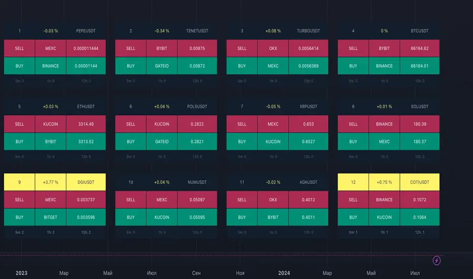
ArbitrageDashboardv3310824This indicator allows you to monitor the spread (difference in exchange rates) between two assets in real-time for up to 12 trading pairs simultaneously.
⚙️ How does the indicator work?
In the settings menu, you can select two trading pairs, such as BTCUSDT on Binance and BTCUSDT on Bybit. The script then fetches prices from both exchanges and compares them, calculating the percentage difference (spread). This process is repeated for all 12 trading pairs added in the settings. The script works only with the assets and exchanges available on TradingView.
⚡️ How to use it?
When the spread is negative, it means the asset's price on the first exchange is lower than on the second. By buying on the first exchange and selling on the second, you can make a profit (taking into account the exchange fees). When the spread is positive, the opposite is true. The buy prices and exchanges are shown in a green Buy row, while sell prices and exchanges are displayed in a red Sell row. If the spread is zero, prices are the same on both exchanges, and no arbitrage opportunity exists. For better accuracy, use the smallest timeframe available in your TradingView subscription, such as minute or second intervals.
🕒 Arbitrage Situation Counter
For each trading pair, the table below the Buy row shows the number of arbitrage situations within a specified timeframe. An arbitrage situation occurs when the spread exceeds the Signal Threshold Level set by the user. Each time this happens, the counter increases by one. It only counts situations that occurred within the selected timeframe, such as the past hour for a 1-hour period. You can track arbitrage situations for up to three different periods simultaneously, ranging from 5 minutes to 24 hours. This counter helps evaluate the potential for arbitrage in the selected trading pairs. If a pair shows only 1-2 arbitrage situations per hour, it might be better to look for another pair.
🔔 Setting Up Alerts
In the script settings, you can set the Spread Signal Threshold. When the spread reaches this level, the table for that asset will be highlighted. This threshold also acts as a signal for setting up alerts. To set alerts, go to the Alerts tab in the TradingView menu on the right, click "Create Alert", and select this indicator under "Condition". You can then name the alert and finish the setup by clicking "Create".
We, the authors, have long been involved in cryptocurrency arbitrage and created this script for our own trading, but you can use it for any assets and markets as you see fit.
We also offer lighter versions of the indicator that track the spread for one or three trading pairs. These versions also display the spread chart, which can be useful for historical analysis. If the full indicator is too resource-intensive for your device, try these lighter versions:
🧩 Arbitrage Spread v1 : 1 pair + 1 chart
🧩 Arbitrage Spread v2 : 3 pairs + 3 charts
If your hardware can handle it, you can use the 12-pair version as a dashboard and add one of the versions with a spread chart for a detailed view of one or three pairs.
--
Этот индикатор позволяет в реальном времени отслеживать изменение спреда (разницы в цене) между двумя активами для 12 торговых пар одновременно.
⚙️ Как работает индикатор?
В меню настроек индикатора пользователь выбирает две торговые пары, например BTCUSDT на бирже Binance и BTCUSDT на бирже Bybit. Скрипт получает цены с обеих бирж и сравнивает их, рассчитывая процентное отклонение (спред). Этот процесс выполняется для всех 12 торговых пар, указанных в настройках. Скрипт работает только с теми активами и биржами, которые доступны на TradingView.
⚡️ Как использовать?
Когда спред отрицательный, это означает, что цена на первый актив ниже, чем на второй. В таком случае можно купить актив на первой бирже и продать на второй, получив прибыль (не забывая учитывать биржевые комиссии). Когда спред положительный, ситуация обратная. Биржи и цены для покупки отображаются в зеленой строке Buy, а для продажи – в красной строке Sell. При нулевом спреде цены на обеих биржах одинаковы, и арбитражная ситуация отсутствует.
Для повышения точности индикатора используйте минимально доступный таймфрейм на TradingView – минутный или секундный.
🕒 Счетчик арбитражных ситуаций
По каждой торговой паре в таблице под строкой Buy отображается количество арбитражных ситуаций за определенный промежуток времени. Арбитражная ситуация возникает, когда спред превышает установленный пользователем сигнальный уровень (Signal Threshold Level). При каждом превышении этого уровня счетчик увеличивается на единицу. Счетчик учитывает арбитражные ситуации за определенный период, например, за последний час для 1-часового периода (1h). Можно отслеживать количество арбитражных ситуаций одновременно для трех временных периодов от 5 минут до суток.
Счетчик помогает оценить перспективность арбитража выбранных пар. Если за час на паре было всего 1-2 арбитражные ситуации, возможно, лучше поискать другую пару.
🔔 Настройка оповещений
В настройках скрипта можно задать пороговое значение спреда (Spread Signal Threshold). Когда спред достигнет этого уровня, таблица для данного актива будет подсвечена. Этот уровень также служит сигналом для настройки оповещений.
Для настройки оповещений откройте вкладку «Оповещения» в меню TradingView справа. Нажмите кнопку «Создать оповещение». В открывшемся окне в строке «Условие» выберите данный индикатор. Затем задайте название и завершите настройку, нажав кнопку «Создать».
Мы, авторы этого скрипта, давно занимаемся арбитражем криптовалют и создали его для себя, но вы можете использовать его для любых активов и на любых рынках по своему усмотрению.
У нас также есть более простая версия индикатора, которая отслеживает спред для одной или трех торговых пар. В этих версиях можно просматривать график самого спреда, что полезно для оценки его динамики. Если этот индикатор кажется вам или вашему устройству слишком тяжелым, вы можете воспользоваться облегченными версиями:
🧩 Arbitrage Spread v1 : 1 пара + 1 график
🧩 Arbitrage Spread v2 : 3 пары + 3 графика
Если ваше оборудование позволяет, вы можете добавить несколько индикаторов на экран. Например, использовать версию с 12 парами как дашборд, а одну из версий с графиком спреда для более детального анализа по одному или трем инструментам.
PubLibTrendLibrary "PubLibTrend"
trend, multi-part trend, double trend and multi-part double trend conditions for indicator and strategy development
rlut()
return line uptrend condition
Returns: bool
dt()
downtrend condition
Returns: bool
ut()
uptrend condition
Returns: bool
rldt()
return line downtrend condition
Returns: bool
dtop()
double top condition
Returns: bool
dbot()
double bottom condition
Returns: bool
rlut_1p()
1-part return line uptrend condition
Returns: bool
rlut_2p()
2-part return line uptrend condition
Returns: bool
rlut_3p()
3-part return line uptrend condition
Returns: bool
rlut_4p()
4-part return line uptrend condition
Returns: bool
rlut_5p()
5-part return line uptrend condition
Returns: bool
rlut_6p()
6-part return line uptrend condition
Returns: bool
rlut_7p()
7-part return line uptrend condition
Returns: bool
rlut_8p()
8-part return line uptrend condition
Returns: bool
rlut_9p()
9-part return line uptrend condition
Returns: bool
rlut_10p()
10-part return line uptrend condition
Returns: bool
rlut_11p()
11-part return line uptrend condition
Returns: bool
rlut_12p()
12-part return line uptrend condition
Returns: bool
rlut_13p()
13-part return line uptrend condition
Returns: bool
rlut_14p()
14-part return line uptrend condition
Returns: bool
rlut_15p()
15-part return line uptrend condition
Returns: bool
rlut_16p()
16-part return line uptrend condition
Returns: bool
rlut_17p()
17-part return line uptrend condition
Returns: bool
rlut_18p()
18-part return line uptrend condition
Returns: bool
rlut_19p()
19-part return line uptrend condition
Returns: bool
rlut_20p()
20-part return line uptrend condition
Returns: bool
rlut_21p()
21-part return line uptrend condition
Returns: bool
rlut_22p()
22-part return line uptrend condition
Returns: bool
rlut_23p()
23-part return line uptrend condition
Returns: bool
rlut_24p()
24-part return line uptrend condition
Returns: bool
rlut_25p()
25-part return line uptrend condition
Returns: bool
rlut_26p()
26-part return line uptrend condition
Returns: bool
rlut_27p()
27-part return line uptrend condition
Returns: bool
rlut_28p()
28-part return line uptrend condition
Returns: bool
rlut_29p()
29-part return line uptrend condition
Returns: bool
rlut_30p()
30-part return line uptrend condition
Returns: bool
dt_1p()
1-part downtrend condition
Returns: bool
dt_2p()
2-part downtrend condition
Returns: bool
dt_3p()
3-part downtrend condition
Returns: bool
dt_4p()
4-part downtrend condition
Returns: bool
dt_5p()
5-part downtrend condition
Returns: bool
dt_6p()
6-part downtrend condition
Returns: bool
dt_7p()
7-part downtrend condition
Returns: bool
dt_8p()
8-part downtrend condition
Returns: bool
dt_9p()
9-part downtrend condition
Returns: bool
dt_10p()
10-part downtrend condition
Returns: bool
dt_11p()
11-part downtrend condition
Returns: bool
dt_12p()
12-part downtrend condition
Returns: bool
dt_13p()
13-part downtrend condition
Returns: bool
dt_14p()
14-part downtrend condition
Returns: bool
dt_15p()
15-part downtrend condition
Returns: bool
dt_16p()
16-part downtrend condition
Returns: bool
dt_17p()
17-part downtrend condition
Returns: bool
dt_18p()
18-part downtrend condition
Returns: bool
dt_19p()
19-part downtrend condition
Returns: bool
dt_20p()
20-part downtrend condition
Returns: bool
dt_21p()
21-part downtrend condition
Returns: bool
dt_22p()
22-part downtrend condition
Returns: bool
dt_23p()
23-part downtrend condition
Returns: bool
dt_24p()
24-part downtrend condition
Returns: bool
dt_25p()
25-part downtrend condition
Returns: bool
dt_26p()
26-part downtrend condition
Returns: bool
dt_27p()
27-part downtrend condition
Returns: bool
dt_28p()
28-part downtrend condition
Returns: bool
dt_29p()
29-part downtrend condition
Returns: bool
dt_30p()
30-part downtrend condition
Returns: bool
ut_1p()
1-part uptrend condition
Returns: bool
ut_2p()
2-part uptrend condition
Returns: bool
ut_3p()
3-part uptrend condition
Returns: bool
ut_4p()
4-part uptrend condition
Returns: bool
ut_5p()
5-part uptrend condition
Returns: bool
ut_6p()
6-part uptrend condition
Returns: bool
ut_7p()
7-part uptrend condition
Returns: bool
ut_8p()
8-part uptrend condition
Returns: bool
ut_9p()
9-part uptrend condition
Returns: bool
ut_10p()
10-part uptrend condition
Returns: bool
ut_11p()
11-part uptrend condition
Returns: bool
ut_12p()
12-part uptrend condition
Returns: bool
ut_13p()
13-part uptrend condition
Returns: bool
ut_14p()
14-part uptrend condition
Returns: bool
ut_15p()
15-part uptrend condition
Returns: bool
ut_16p()
16-part uptrend condition
Returns: bool
ut_17p()
17-part uptrend condition
Returns: bool
ut_18p()
18-part uptrend condition
Returns: bool
ut_19p()
19-part uptrend condition
Returns: bool
ut_20p()
20-part uptrend condition
Returns: bool
ut_21p()
21-part uptrend condition
Returns: bool
ut_22p()
22-part uptrend condition
Returns: bool
ut_23p()
23-part uptrend condition
Returns: bool
ut_24p()
24-part uptrend condition
Returns: bool
ut_25p()
25-part uptrend condition
Returns: bool
ut_26p()
26-part uptrend condition
Returns: bool
ut_27p()
27-part uptrend condition
Returns: bool
ut_28p()
28-part uptrend condition
Returns: bool
ut_29p()
29-part uptrend condition
Returns: bool
ut_30p()
30-part uptrend condition
Returns: bool
rldt_1p()
1-part return line downtrend condition
Returns: bool
rldt_2p()
2-part return line downtrend condition
Returns: bool
rldt_3p()
3-part return line downtrend condition
Returns: bool
rldt_4p()
4-part return line downtrend condition
Returns: bool
rldt_5p()
5-part return line downtrend condition
Returns: bool
rldt_6p()
6-part return line downtrend condition
Returns: bool
rldt_7p()
7-part return line downtrend condition
Returns: bool
rldt_8p()
8-part return line downtrend condition
Returns: bool
rldt_9p()
9-part return line downtrend condition
Returns: bool
rldt_10p()
10-part return line downtrend condition
Returns: bool
rldt_11p()
11-part return line downtrend condition
Returns: bool
rldt_12p()
12-part return line downtrend condition
Returns: bool
rldt_13p()
13-part return line downtrend condition
Returns: bool
rldt_14p()
14-part return line downtrend condition
Returns: bool
rldt_15p()
15-part return line downtrend condition
Returns: bool
rldt_16p()
16-part return line downtrend condition
Returns: bool
rldt_17p()
17-part return line downtrend condition
Returns: bool
rldt_18p()
18-part return line downtrend condition
Returns: bool
rldt_19p()
19-part return line downtrend condition
Returns: bool
rldt_20p()
20-part return line downtrend condition
Returns: bool
rldt_21p()
21-part return line downtrend condition
Returns: bool
rldt_22p()
22-part return line downtrend condition
Returns: bool
rldt_23p()
23-part return line downtrend condition
Returns: bool
rldt_24p()
24-part return line downtrend condition
Returns: bool
rldt_25p()
25-part return line downtrend condition
Returns: bool
rldt_26p()
26-part return line downtrend condition
Returns: bool
rldt_27p()
27-part return line downtrend condition
Returns: bool
rldt_28p()
28-part return line downtrend condition
Returns: bool
rldt_29p()
29-part return line downtrend condition
Returns: bool
rldt_30p()
30-part return line downtrend condition
Returns: bool
dut()
double uptrend condition
Returns: bool
ddt()
double downtrend condition
Returns: bool
dut_1p()
1-part double uptrend condition
Returns: bool
dut_2p()
2-part double uptrend condition
Returns: bool
dut_3p()
3-part double uptrend condition
Returns: bool
dut_4p()
4-part double uptrend condition
Returns: bool
dut_5p()
5-part double uptrend condition
Returns: bool
dut_6p()
6-part double uptrend condition
Returns: bool
dut_7p()
7-part double uptrend condition
Returns: bool
dut_8p()
8-part double uptrend condition
Returns: bool
dut_9p()
9-part double uptrend condition
Returns: bool
dut_10p()
10-part double uptrend condition
Returns: bool
dut_11p()
11-part double uptrend condition
Returns: bool
dut_12p()
12-part double uptrend condition
Returns: bool
dut_13p()
13-part double uptrend condition
Returns: bool
dut_14p()
14-part double uptrend condition
Returns: bool
dut_15p()
15-part double uptrend condition
Returns: bool
dut_16p()
16-part double uptrend condition
Returns: bool
dut_17p()
17-part double uptrend condition
Returns: bool
dut_18p()
18-part double uptrend condition
Returns: bool
dut_19p()
19-part double uptrend condition
Returns: bool
dut_20p()
20-part double uptrend condition
Returns: bool
dut_21p()
21-part double uptrend condition
Returns: bool
dut_22p()
22-part double uptrend condition
Returns: bool
dut_23p()
23-part double uptrend condition
Returns: bool
dut_24p()
24-part double uptrend condition
Returns: bool
dut_25p()
25-part double uptrend condition
Returns: bool
dut_26p()
26-part double uptrend condition
Returns: bool
dut_27p()
27-part double uptrend condition
Returns: bool
dut_28p()
28-part double uptrend condition
Returns: bool
dut_29p()
29-part double uptrend condition
Returns: bool
dut_30p()
30-part double uptrend condition
Returns: bool
ddt_1p()
1-part double downtrend condition
Returns: bool
ddt_2p()
2-part double downtrend condition
Returns: bool
ddt_3p()
3-part double downtrend condition
Returns: bool
ddt_4p()
4-part double downtrend condition
Returns: bool
ddt_5p()
5-part double downtrend condition
Returns: bool
ddt_6p()
6-part double downtrend condition
Returns: bool
ddt_7p()
7-part double downtrend condition
Returns: bool
ddt_8p()
8-part double downtrend condition
Returns: bool
ddt_9p()
9-part double downtrend condition
Returns: bool
ddt_10p()
10-part double downtrend condition
Returns: bool
ddt_11p()
11-part double downtrend condition
Returns: bool
ddt_12p()
12-part double downtrend condition
Returns: bool
ddt_13p()
13-part double downtrend condition
Returns: bool
ddt_14p()
14-part double downtrend condition
Returns: bool
ddt_15p()
15-part double downtrend condition
Returns: bool
ddt_16p()
16-part double downtrend condition
Returns: bool
ddt_17p()
17-part double downtrend condition
Returns: bool
ddt_18p()
18-part double downtrend condition
Returns: bool
ddt_19p()
19-part double downtrend condition
Returns: bool
ddt_20p()
20-part double downtrend condition
Returns: bool
ddt_21p()
21-part double downtrend condition
Returns: bool
ddt_22p()
22-part double downtrend condition
Returns: bool
ddt_23p()
23-part double downtrend condition
Returns: bool
ddt_24p()
24-part double downtrend condition
Returns: bool
ddt_25p()
25-part double downtrend condition
Returns: bool
ddt_26p()
26-part double downtrend condition
Returns: bool
ddt_27p()
27-part double downtrend condition
Returns: bool
ddt_28p()
28-part double downtrend condition
Returns: bool
ddt_29p()
29-part double downtrend condition
Returns: bool
ddt_30p()
30-part double downtrend condition
Returns: bool

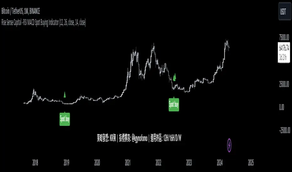
Rise Sense Capital - RSI MACD Spot Buying IndicatorToday, I'll share a spot buying strategy shared by a member @KR陳 within the DATA Trader Alliance Alpha group. First, you need to prepare two indicators:
今天分享一個DATA交易者聯盟Alpha群組裏面的群友@KR陳分享的現貨買入策略。
首先需要準備兩個指標
RSI Indicator (Relative Strength Index) - RSI is a technical analysis tool based on price movements over a period of time to evaluate the speed and magnitude of price changes. RSI calculates the changes in price over a period to determine whether the recent trend is relatively strong (bullish) or weak (bearish).
RSI指標,(英文全名:Relative Strength Index),中文稱為「相對強弱指標」,是一種以股價漲跌為基礎,在一段時間內的收盤價,用於評估價格變動的速度 (快慢) 與變化 (幅度) 的技術分析工具,RSI藉由計算一段期間內股價的漲跌變化,判斷最近的趨勢屬於偏強 (偏多) 還是偏弱 (偏空)。
MACD Indicator (Moving Average Convergence & Divergence) - MACD is a technical analysis tool proposed by Gerald Appel in the 1970s. It is commonly used in trading to determine trend reversals by analyzing the convergence and divergence of fast and slow lines.
MACD 指標 (Moving Average Convergence & Divergence) 中文名為平滑異同移動平均線指標,MACD 是在 1970 年代由美國人 Gerald Appel 所提出,是一項歷史悠久且經常在交易中被使用的技術分析工具,原理是利用快慢線的交錯,藉以判斷股價走勢的轉折。
In MACD analysis, the most commonly used values are 12, 26, and 9, known as MACD (12,26,9). The market often uses the MACD indicator to determine the future direction of assets and to identify entry and exit points.
在 MACD 的技術分析中,最常用的值為 12 天、26 天、9 天,也稱為 MACD (12,26,9),市場常用 MACD 指標來判斷操作標的的後市走向,確定波段漲幅並找到進、出場點。
Strategy analysis by member KR陳:
策略解析 by群友 KR陳 :
Condition 1: RSI value in the previous candle is below oversold zone(30).
條件1:RSI 在前一根的數值低於超賣區(30)
buycondition1 = RSI <30
Condition 2: MACD histogram changes from decreasing to increasing.
條件2:MACD柱由遞減轉遞增
buycondition2 = hist >hist and hist
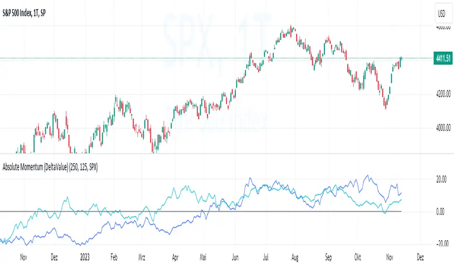
Absolute Momentum (Time Series Momentum)Absolute momentum , also known as time series momentum , focuses on the trend of an asset's own past performance to predict its future performance. It involves analyzing an asset's own historical performance, rather than comparing it to other assets.
The strategy determines whether an asset's price is exhibiting an upward (positive momentum) or downward (negative momentum) trend by assessing the asset's return over a given period (standard look-back period: 12 months or approximately 250 trading days). Some studies recommend calculating momentum by deducting the corresponding Treasury bill rate from the measured performance.
Absolute Momentum Indicator
The Absolute Momentum Indicator displays the rolling 12-month performance (measured over 250 trading days) and plots it against a horizontal line representing 0%. If the indicator crosses above this line, it signifies positive absolute momentum, and conversely, crossing below indicates negative momentum. An additional, optional look-back period input field can be accessed through the settings.
Hint: This indicator is a simplified version, as some academic approaches measure absolute momentum by subtracting risk-free rates from the 12-month performance. However, even with higher rates, the values will still remain close to the 0% line.
Benefits of Absolute Momentum
Absolute momentum, which should not be confused with relative momentum or the momentum indicator, serves as a timing instrument for both individual assets and entire markets.
Gary Antonacci , a key contributor to the absolute momentum strategy (find study below), emphasizes its effectiveness in multi-asset portfolios and its importance in long-only investing. This is particularly evident in a) reducing downside volatility and b) mitigating behavioral biases.
Moskowitz, Ooi, and Pedersen document significant 'time series momentum' across various asset classes, including equity index, currency, commodity, and bond futures, in 58 liquid instruments (find study below). There's a notable persistence in returns ranging from one to 12 months, which tends to partially reverse over longer periods. This pattern aligns with sentiment theories suggesting initial under-reaction followed by delayed over-reaction.
Despite its surprising ease of implementation, the academic community has successfully measured the effects of absolute momentum across decades and in every major asset class, including stocks, bonds, commodities, and foreign exchange (FX).
Strategies for Implementing Absolute Momentum:
To Buy a Stock:
Select a Look-Back Period: Choose a historical period to analyze the stock's performance. A common period is 12 months, but this can vary based on your investment strategy.
Calculate Excess Return: Determine the stock's excess return over this period. You can also assume a risk-free rate of "0" to simplify the process.
Evaluate Momentum:
If the excess return is positive, it indicates positive absolute momentum. This suggests the stock is in an upward trend and could be a good buying opportunity.
If the excess return is negative, it suggests negative momentum, and you might want to delay buying.
Consider further conditions: Align your decision with broader market trends, economic indicators, or fundamental analysis, for additional context.
To Sell a Stock You Own:
Regularly Monitor Performance: Use the same look-back period as for buying (e.g., 12 months) to regularly assess the stock's performance.
Check for Negative Momentum: Calculate the excess return for the look-back period. Again, you can assume a risk-free rate of "0" to simplify the process. If the stock shows negative momentum, it might be time to consider selling.
Consider further conditions:Align your decision with broader market trends, economic indicators, or fundamental analysis, for additional context.
Important note: Note: Entering a position (i.e., buying) based on positive absolute momentum doesn't necessarily mean you must sell it if it later exhibits negative absolute momentum. You can initiate a position using positive absolute momentum as an entry indicator and then continue holding it based on other criteria, such as fundamental analysis.
General Tips:
Reassessment Frequency: Decide how often you will reassess the momentum (monthly, quarterly, etc.).
Remember, while absolute momentum provides a systematic approach, it's recommendable to consider it as part of a broader investment strategy that includes diversification, risk management, fundamental analysis, etc.
Relevant Capital Market Studies:
Antonacci, Gary. "Absolute momentum: A simple rule-based strategy and universal trend-following overlay." Available at SSRN 2244633 (2013)
Moskowitz, Tobias J., Yao Hua Ooi, and Lasse Heje Pedersen. "Time series momentum." Journal of financial economics 104.2 (2012): 228-250
S&P 500 Quandl Data & RatiosTradingView has a little-known integration that allows you to pull in 3rd party data-sets from Nasdaq Data Link, also known as Quandl. Today, I am open-sourcing for the community an indicator that uses the Quandl integration to pull in historical data and ratios on the S&P500. I originally coded this to study macro P/E ratios during peaks and troughs of boom/bust cycles.
The indicator pulls in each of the following datasets, as defined and provided by Quandl. The user can select which datasets to pull in using the indicator settings:
Dividend Yield : S&P 500 dividend yield (12 month dividend per share)/price. Yields following June 2022 (including the current yield) are estimated based on 12 month dividends through June 2022, as reported by S&P. Sources: Standard & Poor's for current S&P 500 Dividend Yield. Robert Shiller and his book Irrational Exuberance for historic S&P 500 Dividend Yields.
Price Earning Ratio : Price to earnings ratio, based on trailing twelve month as reported earnings. Current PE is estimated from latest reported earnings and current market price. Source: Robert Shiller and his book Irrational Exuberance for historic S&P 500 PE Ratio.
CAPE/Shiller PE Ratio : Shiller PE ratio for the S&P 500. Price earnings ratio is based on average inflation-adjusted earnings from the previous 10 years, known as the Cyclically Adjusted PE Ratio (CAPE Ratio), Shiller PE Ratio, or PE 10 FAQ. Data courtesy of Robert Shiller from his book, Irrational Exuberance.
Earnings Yield : S&P 500 Earnings Yield. Earnings Yield = trailing 12 month earnings divided by index price (or inverse PE) Yields following March, 2022 (including current yield) are estimated based on 12 month earnings through March, 2022 the latest reported by S&P. Source: Standard & Poor's
Price Book Ratio : S&P 500 price to book value ratio. Current price to book ratio is estimated based on current market price and S&P 500 book value as of March, 2022 the latest reported by S&P. Source: Standard & Poor's
Price Sales Ratio : S&P 500 Price to Sales Ratio (P/S or Price to Revenue). Current price to sales ratio is estimated based on current market price and 12 month sales ending March, 2022 the latest reported by S&P. Source: Standard & Poor's
Inflation Adjusted SP500 : Inflation adjusted SP500. Other than the current price, all prices are monthly average closing prices. Sources: Standard & Poor's Robert Shiller and his book Irrational Exuberance for historic S&P 500 prices, and historic CPIs.
Revenue Per Share : Trailing twelve month S&P 500 Sales Per Share (S&P 500 Revenue Per Share) non-inflation adjusted current dollars. Source: Standard & Poor's
Earnings Per Share : S&P 500 Earnings Per Share. 12-month real earnings per share inflation adjusted, constant August, 2022 dollars. Sources: Standard & Poor's for current S&P 500 Earnings. Robert Shiller and his book Irrational Exuberance for historic S&P 500 Earnings.
Disclaimer: This is not financial advice. Open-source scripts I publish in the community are largely meant to spark ideas that can be used as building blocks for part of a more robust trade management strategy. If you would like to implement a version of any script, I would recommend making significant additions/modifications to the strategy & risk management functions. If you don’t know how to program in Pine, then hire a Pine-coder. We can help!

Argo II - (alerts for 3commas composite bots) - publicThis script lets users create BUY/SELL alerts for 3commas composite bots (1 alert = 12 pairs) in a simple way, based on a built in set of indicators that can be tweaked to work together or alone through the study settings.
There is a version of this script for single pair bots, with slightly more features here .
If the user choses to create both BUY and SELL signals from the study settings, the (1) alert created will send both BUY and SELL signals for all 12 pairs selected. At this stage, the script forces the user to select 12 pairs in the study settings. If less pairs are inserted, it will not work. Also, the script will only send alerts for the pairs selected in the study settings, not for the current chart (if different).
How to use:
- Add the script to the current chart
- Open the study settings , insert bot details and select 12 pairs. You should write the pairs manually, using the format BTC , ADA, ETH, etc. They MUST be in capital letters or 3commas will not recognize them.
- Still in the study settings, tweak the deal start/close conditions from various indicators until happy. The study will plot the entry / exit points below the current chart (1 = buy, 2 = sell)
- Make sure your strategy works for all the pairs you have selected, simply by checking each chart with the same study settings
- When happy, right click on the "..." next to the study name, then "Add alert'".
- Under "Condition", on the second line, chose "Any alert () function call". Add the webhook from 3commas, give it a name, and "create".
That's it.
Notes:
- If you insert coins that are not available for the quote currency and exchange of your choosing, the script will not work and return an error.
- Make sure you run tests with paper trading or dummy bots (i.e without actual bot ID) to ensure your alerts trigger as intended on all coins.
- If alerts trigger too much (i.e they all trigger at the same time for all coins), Trading View will stop the alert. So probably not ideal for a scalping bot. It could also be the sign the script doesn't work as intended.
- The script is a bit slow on my side. I am a beginner in pinescript, so if anyone knows how to simplify it, please let me know.
- if anyone knows how to tell the script to function with less than 12 pairs (when not filling the 12 fields in the setting), please also let me know :)
XPloRR MA-Buy ATR-Trailing-Stop Long Term Strategy Beating B&HXPloRR MA-Buy ATR-MA-Trailing-Stop Strategy
Long term MA Trailing Stop strategy to beat Buy&Hold strategy
None of the strategies that I tested can beat the long term Buy&Hold strategy. That's the reason why I wrote this strategy.
Purpose: beat Buy&Hold strategy with around 10 trades. 100% capitalize sold trade into new trade.
My buy strategy is triggered by the EMA(blue) crossing over the SMA curve(orange).
My sell strategy is triggered by another EMA(lime) of the close value crossing the trailing stop(green) value.
The trailing stop value(green) is set to a multiple of the ATR(15) value.
ATR(15) is the SMA(15) value of the difference between high and low values.
Every stock has it's own "DNA", so first thing to do is find the right parameters to get the best strategy values voor EMA, SMA and Trailing Stop.
Then keep using these parameter for future buy/sell signals only for that particular stock.
Do the same for other stocks.
Here are the parameters:
Exponential MA: buy trigger when crossing over the SMA value (use values between 11-50)
Simple MA: buy trigger when EMA crosses over the SMA value (use values between 20 and 200)
Stop EMA: sell trigger when Stop EMA of close value crosses under the trailing stop value (use values between 8 and 16)
Trailing Stop #ATR: defines the trailing stop value as a multiple of the ATR(15) value
Example parameters for different stocks (Start capital: 1000, Order=100% of equity, Period 1/1/2005 to now):
BAR(Barco): EMA=11, SMA=82, StopEMA=12, Stop#ATR=9
Buy&HoldProfit: 45.82%, NetProfit: 294.7%, #Trades:8, %Profit:62.5%, ProfitFactor: 12.539
AAPL(Apple): EMA=12, SMA=45, StopEMA=12, Stop#ATR=6
Buy&HoldProfit: 2925.86%, NetProfit: 4035.92%, #Trades:10, %Profit:60%, ProfitFactor: 6.36
BEKB(Bekaert): EMA=12, SMA=42, StopEMA=12, Stop#ATR=7
Buy&HoldProfit: 81.11%, NetProfit: 521.37%, #Trades:10, %Profit:60%, ProfitFactor: 2.617
SOLB(Solvay): EMA=12, SMA=63, StopEMA=11, Stop#ATR=8
Buy&HoldProfit: 43.61%, NetProfit: 151.4%, #Trades:8, %Profit:75%, ProfitFactor: 3.794
PHIA(Philips): EMA=11, SMA=80, StopEMA=8, Stop#ATR=10
Buy&HoldProfit: 56.79%, NetProfit: 198.46%, #Trades:6, %Profit:83.33%, ProfitFactor: 23.07
I am very curious to see the parameters for your stocks and please make suggestions to improve this strategy.

Adaptive Genesis Engine [AGE]ADAPTIVE GENESIS ENGINE (AGE)
Pure Signal Evolution Through Genetic Algorithms
Where Darwin Meets Technical Analysis
🧬 WHAT YOU'RE GETTING - THE PURE INDICATOR
This is a technical analysis indicator - it generates signals, visualizes probability, and shows you the evolutionary process in real-time. This is NOT a strategy with automatic execution - it's a sophisticated signal generation system that you control .
What This Indicator Does:
Generates Long/Short entry signals with probability scores (35-88% range)
Evolves a population of up to 12 competing strategies using genetic algorithms
Validates strategies through walk-forward optimization (train/test cycles)
Visualizes signal quality through premium gradient clouds and confidence halos
Displays comprehensive metrics via enhanced dashboard
Provides alerts for entries and exits
Works on any timeframe, any instrument, any broker
What This Indicator Does NOT Do:
Execute trades automatically
Manage positions or calculate position sizes
Place orders on your behalf
Make trading decisions for you
This is pure signal intelligence. AGE tells you when and how confident it is. You decide whether and how much to trade.
🔬 THE SCIENCE: GENETIC ALGORITHMS MEET TECHNICAL ANALYSIS
What Makes This Different - The Evolutionary Foundation
Most indicators are static - they use the same parameters forever, regardless of market conditions. AGE is alive . It maintains a population of competing strategies that evolve, adapt, and improve through natural selection principles:
Birth: New strategies spawn through crossover breeding (combining DNA from fit parents) plus random mutation for exploration
Life: Each strategy trades virtually via shadow portfolios, accumulating wins/losses, tracking drawdown, and building performance history
Selection: Strategies are ranked by comprehensive fitness scoring (win rate, expectancy, drawdown control, signal efficiency)
Death: Weak strategies are culled periodically, with elite performers (top 2 by default) protected from removal
Evolution: The gene pool continuously improves as successful traits propagate and unsuccessful ones die out
This is not curve-fitting. Each new strategy must prove itself on out-of-sample data through walk-forward validation before being trusted for live signals.
🧪 THE DNA: WHAT EVOLVES
Every strategy carries a 10-gene chromosome controlling how it interprets market data:
Signal Sensitivity Genes
Entropy Sensitivity (0.5-2.0): Weight given to market order/disorder calculations. Low values = conservative, require strong directional clarity. High values = aggressive, act on weaker order signals.
Momentum Sensitivity (0.5-2.0): Weight given to RSI/ROC/MACD composite. Controls responsiveness to momentum shifts vs. mean-reversion setups.
Structure Sensitivity (0.5-2.0): Weight given to support/resistance positioning. Determines how much price location within swing range matters.
Probability Adjustment Genes
Probability Boost (-0.10 to +0.10): Inherent bias toward aggressive (+) or conservative (-) entries. Acts as personality trait - some strategies naturally optimistic, others pessimistic.
Trend Strength Requirement (0.3-0.8): Minimum trend conviction needed before signaling. Higher values = only trades strong trends, lower values = acts in weak/sideways markets.
Volume Filter (0.5-1.5): Strictness of volume confirmation. Higher values = requires strong volume, lower values = volume less important.
Risk Management Genes
ATR Multiplier (1.5-4.0): Base volatility scaling for all price levels. Controls whether strategy uses tight or wide stops/targets relative to ATR.
Stop Multiplier (1.0-2.5): Stop loss tightness. Lower values = aggressive profit protection, higher values = more breathing room.
Target Multiplier (1.5-4.0): Profit target ambition. Lower values = quick scalping exits, higher values = swing trading holds.
Adaptation Gene
Regime Adaptation (0.0-1.0): How much strategy adjusts behavior based on detected market regime (trending/volatile/choppy). Higher values = more reactive to regime changes.
The Magic: AGE doesn't just try random combinations. Through tournament selection and fitness-weighted crossover, successful gene combinations spread through the population while unsuccessful ones fade away. Over 50-100 bars, you'll see the population converge toward genes that work for YOUR instrument and timeframe.
📊 THE SIGNAL ENGINE: THREE-LAYER SYNTHESIS
Before any strategy generates a signal, AGE calculates probability through multi-indicator confluence:
Layer 1 - Market Entropy (Information Theory)
Measures whether price movements exhibit directional order or random walk characteristics:
The Math:
Shannon Entropy = -Σ(p × log(p))
Market Order = 1 - (Entropy / 0.693)
What It Means:
High entropy = choppy, random market → low confidence signals
Low entropy = directional market → high confidence signals
Direction determined by up-move vs down-move dominance over lookback period (default: 20 bars)
Signal Output: -1.0 to +1.0 (bearish order to bullish order)
Layer 2 - Momentum Synthesis
Combines three momentum indicators into single composite score:
Components:
RSI (40% weight): Normalized to -1/+1 scale using (RSI-50)/50
Rate of Change (30% weight): Percentage change over lookback (default: 14 bars), clamped to ±1
MACD Histogram (30% weight): Fast(12) - Slow(26), normalized by ATR
Why This Matters: RSI catches mean-reversion opportunities, ROC catches raw momentum, MACD catches momentum divergence. Weighting favors RSI for reliability while keeping other perspectives.
Signal Output: -1.0 to +1.0 (strong bearish to strong bullish)
Layer 3 - Structure Analysis
Evaluates price position within swing range (default: 50-bar lookback):
Position Classification:
Bottom 20% of range = Support Zone → bullish bounce potential
Top 20% of range = Resistance Zone → bearish rejection potential
Middle 60% = Neutral Zone → breakout/breakdown monitoring
Signal Logic:
At support + bullish candle = +0.7 (strong buy setup)
At resistance + bearish candle = -0.7 (strong sell setup)
Breaking above range highs = +0.5 (breakout confirmation)
Breaking below range lows = -0.5 (breakdown confirmation)
Consolidation within range = ±0.3 (weak directional bias)
Signal Output: -1.0 to +1.0 (bearish structure to bullish structure)
Confluence Voting System
Each layer casts a vote (Long/Short/Neutral). The system requires minimum 2-of-3 agreement (configurable 1-3) before generating a signal:
Examples:
Entropy: Bullish, Momentum: Bullish, Structure: Neutral → Signal generated (2 long votes)
Entropy: Bearish, Momentum: Neutral, Structure: Neutral → No signal (only 1 short vote)
All three bullish → Signal generated with +5% probability bonus
This is the key to quality. Single indicators give too many false signals. Triple confirmation dramatically improves accuracy.
📈 PROBABILITY CALCULATION: HOW CONFIDENCE IS MEASURED
Base Probability:
Raw_Prob = 50% + (Average_Signal_Strength × 25%)
Then AGE applies strategic adjustments:
Trend Alignment:
Signal with trend: +4%
Signal against strong trend: -8%
Weak/no trend: no adjustment
Regime Adaptation:
Trending market (efficiency >50%, moderate vol): +3%
Volatile market (vol ratio >1.5x): -5%
Choppy market (low efficiency): -2%
Volume Confirmation:
Volume > 70% of 20-bar SMA: no change
Volume below threshold: -3%
Volatility State (DVS Ratio):
High vol (>1.8x baseline): -4% (reduce confidence in chaos)
Low vol (<0.7x baseline): -2% (markets can whipsaw in compression)
Moderate elevated vol (1.0-1.3x): +2% (trending conditions emerging)
Confluence Bonus:
All 3 indicators agree: +5%
2 of 3 agree: +2%
Strategy Gene Adjustment:
Probability Boost gene: -10% to +10%
Regime Adaptation gene: scales regime adjustments by 0-100%
Final Probability: Clamped between 35% (minimum) and 88% (maximum)
Why These Ranges?
Below 35% = too uncertain, better not to signal
Above 88% = unrealistic, creates overconfidence
Sweet spot: 65-80% for quality entries
🔄 THE SHADOW PORTFOLIO SYSTEM: HOW STRATEGIES COMPETE
Each active strategy maintains a virtual trading account that executes in parallel with real-time data:
Shadow Trading Mechanics
Entry Logic:
Calculate signal direction, probability, and confluence using strategy's unique DNA
Check if signal meets quality gate:
Probability ≥ configured minimum threshold (default: 65%)
Confluence ≥ configured minimum (default: 2 of 3)
Direction is not zero (must be long or short, not neutral)
Verify signal persistence:
Base requirement: 2 bars (configurable 1-5)
Adapts based on probability: high-prob signals (75%+) enter 1 bar faster, low-prob signals need 1 bar more
Adjusts for regime: trending markets reduce persistence by 1, volatile markets add 1
Apply additional filters:
Trend strength must exceed strategy's requirement gene
Regime filter: if volatile market detected, probability must be 72%+ to override
Volume confirmation required (volume > 70% of average)
If all conditions met for required persistence bars, enter shadow position at current close price
Position Management:
Entry Price: Recorded at close of entry bar
Stop Loss: ATR-based distance = ATR × ATR_Mult (gene) × Stop_Mult (gene) × DVS_Ratio
Take Profit: ATR-based distance = ATR × ATR_Mult (gene) × Target_Mult (gene) × DVS_Ratio
Position: +1 (long) or -1 (short), only one at a time per strategy
Exit Logic:
Check if price hit stop (on low) or target (on high) on current bar
Record trade outcome in R-multiples (profit/loss normalized by ATR)
Update performance metrics:
Total trades counter incremented
Wins counter (if profit > 0)
Cumulative P&L updated
Peak equity tracked (for drawdown calculation)
Maximum drawdown from peak recorded
Enter cooldown period (default: 8 bars, configurable 3-20) before next entry allowed
Reset signal age counter to zero
Walk-Forward Tracking:
During position lifecycle, trades are categorized:
Training Phase (first 250 bars): Trade counted toward training metrics
Testing Phase (next 75 bars): Trade counted toward testing metrics (out-of-sample)
Live Phase (after WFO period): Trade counted toward overall metrics
Why Shadow Portfolios?
No lookahead bias (uses only data available at the bar)
Realistic execution simulation (entry on close, stop/target checks on high/low)
Independent performance tracking for true fitness comparison
Allows safe experimentation without risking capital
Each strategy learns from its own experience
🏆 FITNESS SCORING: HOW STRATEGIES ARE RANKED
Fitness is not just win rate. AGE uses a comprehensive multi-factor scoring system:
Core Metrics (Minimum 3 trades required)
Win Rate (30% of fitness):
WinRate = Wins / TotalTrades
Normalized directly (0.0-1.0 scale)
Total P&L (30% of fitness):
Normalized_PnL = (PnL + 300) / 600
Clamped 0.0-1.0. Assumes P&L range of -300R to +300R for normalization scale.
Expectancy (25% of fitness):
Expectancy = Total_PnL / Total_Trades
Normalized_Expectancy = (Expectancy + 30) / 60
Clamped 0.0-1.0. Rewards consistency of profit per trade.
Drawdown Control (15% of fitness):
Normalized_DD = 1 - (Max_Drawdown / 15)
Clamped 0.0-1.0. Penalizes strategies that suffer large equity retracements from peak.
Sample Size Adjustment
Quality Factor:
<50 trades: 1.0 (full weight, small sample)
50-100 trades: 0.95 (slight penalty for medium sample)
100 trades: 0.85 (larger penalty for large sample)
Why penalize more trades? Prevents strategies from gaming the system by taking hundreds of tiny trades to inflate statistics. Favors quality over quantity.
Bonus Adjustments
Walk-Forward Validation Bonus:
if (WFO_Validated):
Fitness += (WFO_Efficiency - 0.5) × 0.1
Strategies proven on out-of-sample data receive up to +10% fitness boost based on test/train efficiency ratio.
Signal Efficiency Bonus (if diagnostics enabled):
if (Signals_Evaluated > 10):
Pass_Rate = Signals_Passed / Signals_Evaluated
Fitness += (Pass_Rate - 0.1) × 0.05
Rewards strategies that generate high-quality signals passing the quality gate, not just profitable trades.
Final Fitness: Clamped at 0.0 minimum (prevents negative fitness values)
Result: Elite strategies typically achieve 0.50-0.75 fitness. Anything above 0.60 is excellent. Below 0.30 is prime candidate for culling.
🔬 WALK-FORWARD OPTIMIZATION: ANTI-OVERFITTING PROTECTION
This is what separates AGE from curve-fitted garbage indicators.
The Three-Phase Process
Every new strategy undergoes a rigorous validation lifecycle:
Phase 1 - Training Window (First 250 bars, configurable 100-500):
Strategy trades normally via shadow portfolio
All trades count toward training performance metrics
System learns which gene combinations produce profitable patterns
Tracks independently: Training_Trades, Training_Wins, Training_PnL
Phase 2 - Testing Window (Next 75 bars, configurable 30-200):
Strategy continues trading without any parameter changes
Trades now count toward testing performance metrics (separate tracking)
This is out-of-sample data - strategy has never seen these bars during "optimization"
Tracks independently: Testing_Trades, Testing_Wins, Testing_PnL
Phase 3 - Validation Check:
Minimum_Trades = 5 (configurable 3-15)
IF (Train_Trades >= Minimum AND Test_Trades >= Minimum):
WR_Efficiency = Test_WinRate / Train_WinRate
Expectancy_Efficiency = Test_Expectancy / Train_Expectancy
WFO_Efficiency = (WR_Efficiency + Expectancy_Efficiency) / 2
IF (WFO_Efficiency >= 0.55): // configurable 0.3-0.9
Strategy.Validated = TRUE
Strategy receives fitness bonus
ELSE:
Strategy receives 30% fitness penalty
ELSE:
Validation deferred (insufficient trades in one or both periods)
What Validation Means
Validated Strategy (Green "✓ VAL" in dashboard):
Performed at least 55% as well on unseen data compared to training data
Gets fitness bonus: +(efficiency - 0.5) × 0.1
Receives priority during tournament selection for breeding
More likely to be chosen as active trading strategy
Unvalidated Strategy (Orange "○ TRAIN" in dashboard):
Failed to maintain performance on test data (likely curve-fitted to training period)
Receives 30% fitness penalty (0.7x multiplier)
Makes strategy prime candidate for culling
Can still trade but with lower selection probability
Insufficient Data (continues collecting):
Hasn't completed both training and testing periods yet
OR hasn't achieved minimum trade count in both periods
Validation check deferred until requirements met
Why 55% Efficiency Threshold?
If a strategy earned 10R during training but only 5.5R during testing, it still proved an edge exists beyond random luck. Requiring 100% efficiency would be unrealistic - market conditions change between periods. But requiring >50% ensures the strategy didn't completely degrade on fresh data.
The Protection: Strategies that work great on historical data but fail on new data are automatically identified and penalized. This prevents the population from being polluted by overfitted strategies that would fail in live trading.
🌊 DYNAMIC VOLATILITY SCALING (DVS): ADAPTIVE STOP/TARGET PLACEMENT
AGE doesn't use fixed stop distances. It adapts to current volatility conditions in real-time.
Four Volatility Measurement Methods
1. ATR Ratio (Simple Method):
Current_Vol = ATR(14) / Close
Baseline_Vol = SMA(Current_Vol, 100)
Ratio = Current_Vol / Baseline_Vol
Basic comparison of current ATR to 100-bar moving average baseline.
2. Parkinson (High-Low Range Based):
For each bar: HL = log(High / Low)
Parkinson_Vol = sqrt(Σ(HL²) / (4 × Period × log(2)))
More stable than close-to-close volatility. Captures intraday range expansion without overnight gap noise.
3. Garman-Klass (OHLC Based):
HL_Term = 0.5 × ²
CO_Term = (2×log(2) - 1) × ²
GK_Vol = sqrt(Σ(HL_Term - CO_Term) / Period)
Most sophisticated estimator. Incorporates all four price points (open, high, low, close) plus gap information.
4. Ensemble Method (Default - Median of All Three):
Ratio_1 = ATR_Current / ATR_Baseline
Ratio_2 = Parkinson_Current / Parkinson_Baseline
Ratio_3 = GK_Current / GK_Baseline
DVS_Ratio = Median(Ratio_1, Ratio_2, Ratio_3)
Why Ensemble?
Takes median to avoid outliers and false spikes
If ATR jumps but range-based methods stay calm, median prevents overreaction
If one method fails, other two compensate
Most robust approach across different market conditions
Sensitivity Scaling
Scaled_Ratio = (Raw_Ratio) ^ Sensitivity
Sensitivity 0.3: Cube root - heavily dampens volatility impact
Sensitivity 0.5: Square root - moderate dampening
Sensitivity 0.7 (Default): Balanced response to volatility changes
Sensitivity 1.0: Linear - full 1:1 volatility impact
Sensitivity 1.5: Exponential - amplified response to volatility spikes
Safety Clamps: Final DVS Ratio always clamped between 0.5x and 2.5x baseline to prevent extreme position sizing or stop placement errors.
How DVS Affects Shadow Trading
Every strategy's stop and target distances are multiplied by the current DVS ratio:
Stop Loss Distance:
Stop_Distance = ATR × ATR_Mult (gene) × Stop_Mult (gene) × DVS_Ratio
Take Profit Distance:
Target_Distance = ATR × ATR_Mult (gene) × Target_Mult (gene) × DVS_Ratio
Example Scenario:
ATR = 10 points
Strategy's ATR_Mult gene = 2.5
Strategy's Stop_Mult gene = 1.5
Strategy's Target_Mult gene = 2.5
DVS_Ratio = 1.4 (40% above baseline volatility - market heating up)
Stop = 10 × 2.5 × 1.5 × 1.4 = 52.5 points (vs. 37.5 in normal vol)
Target = 10 × 2.5 × 2.5 × 1.4 = 87.5 points (vs. 62.5 in normal vol)
Result:
During volatility spikes: Stops automatically widen to avoid noise-based exits, targets extend for bigger moves
During calm periods: Stops tighten for better risk/reward, targets compress for realistic profit-taking
Strategies adapt risk management to match current market behavior
🧬 THE EVOLUTIONARY CYCLE: SPAWN, COMPETE, CULL
Initialization (Bar 1)
AGE begins with 4 seed strategies (if evolution enabled):
Seed Strategy #0 (Balanced):
All sensitivities at 1.0 (neutral)
Zero probability boost
Moderate trend requirement (0.4)
Standard ATR/stop/target multiples (2.5/1.5/2.5)
Mid-level regime adaptation (0.5)
Seed Strategy #1 (Momentum-Focused):
Lower entropy sensitivity (0.7), higher momentum (1.5)
Slight probability boost (+0.03)
Higher trend requirement (0.5)
Tighter stops (1.3), wider targets (3.0)
Seed Strategy #2 (Entropy-Driven):
Higher entropy sensitivity (1.5), lower momentum (0.8)
Slight probability penalty (-0.02)
More trend tolerant (0.6)
Wider stops (1.8), standard targets (2.5)
Seed Strategy #3 (Structure-Based):
Balanced entropy/momentum (0.8/0.9), high structure (1.4)
Slight probability boost (+0.02)
Lower trend requirement (0.35)
Moderate risk parameters (1.6/2.8)
All seeds start with WFO validation bypassed if WFO is disabled, or must validate if enabled.
Spawning New Strategies
Timing (Adaptive):
Historical phase: Every 30 bars (configurable 10-100)
Live phase: Every 200 bars (configurable 100-500)
Automatically switches to live timing when barstate.isrealtime triggers
Conditions:
Current population < max population limit (default: 8, configurable 4-12)
At least 2 active strategies exist (need parents)
Available slot in population array
Selection Process:
Run tournament selection 3 times with different seeds
Each tournament: randomly sample active strategies, pick highest fitness
Best from 3 tournaments becomes Parent 1
Repeat independently for Parent 2
Ensures fit parents but maintains diversity
Crossover Breeding:
For each of 10 genes:
Parent1_Fitness = fitness
Parent2_Fitness = fitness
Weight1 = Parent1_Fitness / (Parent1_Fitness + Parent2_Fitness)
Gene1 = parent1's value
Gene2 = parent2's value
Child_Gene = Weight1 × Gene1 + (1 - Weight1) × Gene2
Fitness-weighted crossover ensures fitter parent contributes more genetic material.
Mutation:
For each gene in child:
IF (random < mutation_rate):
Gene_Range = GENE_MAX - GENE_MIN
Noise = (random - 0.5) × 2 × mutation_strength × Gene_Range
Mutated_Gene = Clamp(Child_Gene + Noise, GENE_MIN, GENE_MAX)
Historical mutation rate: 20% (aggressive exploration)
Live mutation rate: 8% (conservative stability)
Mutation strength: 12% of gene range (configurable 5-25%)
Initialization of New Strategy:
Unique ID assigned (total_spawned counter)
Parent ID recorded
Generation = max(parent generations) + 1
Birth bar recorded (for age tracking)
All performance metrics zeroed
Shadow portfolio reset
WFO validation flag set to false (must prove itself)
Result: New strategy with hybrid DNA enters population, begins trading in next bar.
Competition (Every Bar)
All active strategies:
Calculate their signal based on unique DNA
Check quality gate with their thresholds
Manage shadow positions (entries/exits)
Update performance metrics
Recalculate fitness score
Track WFO validation progress
Strategies compete indirectly through fitness ranking - no direct interaction.
Culling Weak Strategies
Timing (Adaptive):
Historical phase: Every 60 bars (configurable 20-200, should be 2x spawn interval)
Live phase: Every 400 bars (configurable 200-1000, should be 2x spawn interval)
Minimum Adaptation Score (MAS):
Initial MAS = 0.10
MAS decays: MAS × 0.995 every cull cycle
Minimum MAS = 0.03 (floor)
MAS represents the "survival threshold" - strategies below this fitness level are vulnerable.
Culling Conditions (ALL must be true):
Population > minimum population (default: 3, configurable 2-4)
At least one strategy has fitness < MAS
Strategy's age > culling interval (prevents premature culling of new strategies)
Strategy is not in top N elite (default: 2, configurable 1-3)
Culling Process:
Find worst strategy:
For each active strategy:
IF (age > cull_interval):
Fitness = base_fitness
IF (not WFO_validated AND WFO_enabled):
Fitness × 0.7 // 30% penalty for unvalidated
IF (Fitness < MAS AND Fitness < worst_fitness_found):
worst_strategy = this_strategy
worst_fitness = Fitness
IF (worst_strategy found):
Count elite strategies with fitness > worst_fitness
IF (elite_count >= elite_preservation_count):
Deactivate worst_strategy (set active flag = false)
Increment total_culled counter
Elite Protection:
Even if a strategy's fitness falls below MAS, it survives if fewer than N strategies are better. This prevents culling when population is generally weak.
Result: Weak strategies removed from population, freeing slots for new spawns. Gene pool improves over time.
Selection for Display (Every Bar)
AGE chooses one strategy to display signals:
Best fitness = -1
Selected = none
For each active strategy:
Fitness = base_fitness
IF (WFO_validated):
Fitness × 1.3 // 30% bonus for validated strategies
IF (Fitness > best_fitness):
best_fitness = Fitness
selected_strategy = this_strategy
Display selected strategy's signals on chart
Result: Only the highest-fitness (optionally validated-boosted) strategy's signals appear as chart markers. Other strategies trade invisibly in shadow portfolios.
🎨 PREMIUM VISUALIZATION SYSTEM
AGE includes sophisticated visual feedback that standard indicators lack:
1. Gradient Probability Cloud (Optional, Default: ON)
Multi-layer gradient showing signal buildup 2-3 bars before entry:
Activation Conditions:
Signal persistence > 0 (same directional signal held for multiple bars)
Signal probability ≥ minimum threshold (65% by default)
Signal hasn't yet executed (still in "forming" state)
Visual Construction:
7 gradient layers by default (configurable 3-15)
Each layer is a line-fill pair (top line, bottom line, filled between)
Layer spacing: 0.3 to 1.0 × ATR above/below price
Outer layers = faint, inner layers = bright
Color transitions from base to intense based on layer position
Transparency scales with probability (high prob = more opaque)
Color Selection:
Long signals: Gradient from theme.gradient_bull_mid to theme.gradient_bull_strong
Short signals: Gradient from theme.gradient_bear_mid to theme.gradient_bear_strong
Base transparency: 92%, reduces by up to 8% for high-probability setups
Dynamic Behavior:
Cloud grows/shrinks as signal persistence increases/decreases
Redraws every bar while signal is forming
Disappears when signal executes or invalidates
Performance Note: Computationally expensive due to linefill objects. Disable or reduce layers if chart performance degrades.
2. Population Fitness Ribbon (Optional, Default: ON)
Histogram showing fitness distribution across active strategies:
Activation: Only draws on last bar (barstate.islast) to avoid historical clutter
Visual Construction:
10 histogram layers by default (configurable 5-20)
Plots 50 bars back from current bar
Positioned below price at: lowest_low(100) - 1.5×ATR (doesn't interfere with price action)
Each layer represents a fitness threshold (evenly spaced min to max fitness)
Layer Logic:
For layer_num from 0 to ribbon_layers:
Fitness_threshold = min_fitness + (max_fitness - min_fitness) × (layer / layers)
Count strategies with fitness ≥ threshold
Height = ATR × 0.15 × (count / total_active)
Y_position = base_level + ATR × 0.2 × layer
Color = Gradient from weak to strong based on layer position
Line_width = Scaled by height (taller = thicker)
Visual Feedback:
Tall, bright ribbon = healthy population, many fit strategies at high fitness levels
Short, dim ribbon = weak population, few strategies achieving good fitness
Ribbon compression (layers close together) = population converging to similar fitness
Ribbon spread = diverse fitness range, active selection pressure
Use Case: Quick visual health check without opening dashboard. Ribbon growing upward over time = population improving.
3. Confidence Halo (Optional, Default: ON)
Circular polyline around entry signals showing probability strength:
Activation: Draws when new position opens (shadow_position changes from 0 to ±1)
Visual Construction:
20-segment polyline forming approximate circle
Center: Low - 0.5×ATR (long) or High + 0.5×ATR (short)
Radius: 0.3×ATR (low confidence) to 1.0×ATR (elite confidence)
Scales with: (probability - min_probability) / (1.0 - min_probability)
Color Coding:
Elite (85%+): Cyan (theme.conf_elite), large radius, minimal transparency (40%)
Strong (75-85%): Strong green (theme.conf_strong), medium radius, moderate transparency (50%)
Good (65-75%): Good green (theme.conf_good), smaller radius, more transparent (60%)
Moderate (<65%): Moderate green (theme.conf_moderate), tiny radius, very transparent (70%)
Technical Detail:
Uses chart.point array with index-based positioning
5-bar horizontal spread for circular appearance (±5 bars from entry)
Curved=false (Pine Script polyline limitation)
Fill color matches line color but more transparent (88% vs line's transparency)
Purpose: Instant visual probability assessment. No need to check dashboard - halo size/brightness tells the story.
4. Evolution Event Markers (Optional, Default: ON)
Visual indicators of genetic algorithm activity:
Spawn Markers (Diamond, Cyan):
Plots when total_spawned increases on current bar
Location: bottom of chart (location.bottom)
Color: theme.spawn_marker (cyan/bright blue)
Size: tiny
Indicates new strategy just entered population
Cull Markers (X-Cross, Red):
Plots when total_culled increases on current bar
Location: bottom of chart (location.bottom)
Color: theme.cull_marker (red/pink)
Size: tiny
Indicates weak strategy just removed from population
What It Tells You:
Frequent spawning early = population building, active exploration
Frequent culling early = high selection pressure, weak strategies dying fast
Balanced spawn/cull = healthy evolutionary churn
No markers for long periods = stable population (evolution plateaued or optimal genes found)
5. Entry/Exit Markers
Clear visual signals for selected strategy's trades:
Long Entry (Triangle Up, Green):
Plots when selected strategy opens long position (position changes 0 → +1)
Location: below bar (location.belowbar)
Color: theme.long_primary (green/cyan depending on theme)
Transparency: Scales with probability:
Elite (85%+): 0% (fully opaque)
Strong (75-85%): 10%
Good (65-75%): 20%
Acceptable (55-65%): 35%
Size: small
Short Entry (Triangle Down, Red):
Plots when selected strategy opens short position (position changes 0 → -1)
Location: above bar (location.abovebar)
Color: theme.short_primary (red/pink depending on theme)
Transparency: Same scaling as long entries
Size: small
Exit (X-Cross, Orange):
Plots when selected strategy closes position (position changes ±1 → 0)
Location: absolute (at actual exit price if stop/target lines enabled)
Color: theme.exit_color (orange/yellow depending on theme)
Transparency: 0% (fully opaque)
Size: tiny
Result: Clean, probability-scaled markers that don't clutter chart but convey essential information.
6. Stop Loss & Take Profit Lines (Optional, Default: ON)
Visual representation of shadow portfolio risk levels:
Stop Loss Line:
Plots when selected strategy has active position
Level: shadow_stop value from selected strategy
Color: theme.short_primary with 60% transparency (red/pink, subtle)
Width: 2
Style: plot.style_linebr (breaks when no position)
Take Profit Line:
Plots when selected strategy has active position
Level: shadow_target value from selected strategy
Color: theme.long_primary with 60% transparency (green, subtle)
Width: 2
Style: plot.style_linebr (breaks when no position)
Purpose:
Shows where shadow portfolio would exit for stop/target
Helps visualize strategy's risk/reward ratio
Useful for manual traders to set similar levels
Disable for cleaner chart (recommended for presentations)
7. Dynamic Trend EMA
Gradient-colored trend line that visualizes trend strength:
Calculation:
EMA(close, trend_length) - default 50 period (configurable 20-100)
Slope calculated over 10 bars: (current_ema - ema ) / ema × 100
Color Logic:
Trend_direction:
Slope > 0.1% = Bullish (1)
Slope < -0.1% = Bearish (-1)
Otherwise = Neutral (0)
Trend_strength = abs(slope)
Color = Gradient between:
- Neutral color (gray/purple)
- Strong bullish (bright green) if direction = 1
- Strong bearish (bright red) if direction = -1
Gradient factor = trend_strength (0 to 1+ scale)
Visual Behavior:
Faint gray/purple = weak/no trend (choppy conditions)
Light green/red = emerging trend (low strength)
Bright green/red = strong trend (high conviction)
Color intensity = trend strength magnitude
Transparency: 50% (subtle, doesn't overpower price action)
Purpose: Subconscious awareness of trend state without checking dashboard or indicators.
8. Regime Background Tinting (Subtle)
Ultra-low opacity background color indicating detected market regime:
Regime Detection:
Efficiency = directional_movement / total_range (over trend_length bars)
Vol_ratio = current_volatility / average_volatility
IF (efficiency > 0.5 AND vol_ratio < 1.3):
Regime = Trending (1)
ELSE IF (vol_ratio > 1.5):
Regime = Volatile (2)
ELSE:
Regime = Choppy (0)
Background Colors:
Trending: theme.regime_trending (dark green, 92-93% transparency)
Volatile: theme.regime_volatile (dark red, 93% transparency)
Choppy: No tint (normal background)
Purpose:
Subliminal regime awareness
Helps explain why signals are/aren't generating
Trending = ideal conditions for AGE
Volatile = fewer signals, higher thresholds applied
Choppy = mixed signals, lower confidence
Important: Extremely subtle by design. Not meant to be obvious, just subconscious context.
📊 ENHANCED DASHBOARD
Comprehensive real-time metrics in single organized panel (top-right position):
Dashboard Structure (5 columns × 14 rows)
Header Row:
Column 0: "🧬 AGE PRO" + phase indicator (🔴 LIVE or ⏪ HIST)
Column 1: "POPULATION"
Column 2: "PERFORMANCE"
Column 3: "CURRENT SIGNAL"
Column 4: "ACTIVE STRATEGY"
Column 0: Market State
Regime (📈 TREND / 🌊 CHAOS / ➖ CHOP)
DVS Ratio (current volatility scaling factor, format: #.##)
Trend Direction (▲ BULL / ▼ BEAR / ➖ FLAT with color coding)
Trend Strength (0-100 scale, format: #.##)
Column 1: Population Metrics
Active strategies (count / max_population)
Validated strategies (WFO passed / active total)
Current generation number
Total spawned (all-time strategy births)
Total culled (all-time strategy deaths)
Column 2: Aggregate Performance
Total trades across all active strategies
Aggregate win rate (%) - color-coded:
Green (>55%)
Orange (45-55%)
Red (<45%)
Total P&L in R-multiples - color-coded by positive/negative
Best fitness score in population (format: #.###)
MAS - Minimum Adaptation Score (cull threshold, format: #.###)
Column 3: Current Signal Status
Status indicator:
"▲ LONG" (green) if selected strategy in long position
"▼ SHORT" (red) if selected strategy in short position
"⏳ FORMING" (orange) if signal persisting but not yet executed
"○ WAITING" (gray) if no active signal
Confidence percentage (0-100%, format: #.#%)
Quality assessment:
"🔥 ELITE" (cyan) for 85%+ probability
"✓ STRONG" (bright green) for 75-85%
"○ GOOD" (green) for 65-75%
"- LOW" (dim) for <65%
Confluence score (X/3 format)
Signal age:
"X bars" if signal forming
"IN TRADE" if position active
"---" if no signal
Column 4: Selected Strategy Details
Strategy ID number (#X format)
Validation status:
"✓ VAL" (green) if WFO validated
"○ TRAIN" (orange) if still in training/testing phase
Generation number (GX format)
Personal fitness score (format: #.### with color coding)
Trade count
P&L and win rate (format: #.#R (##%) with color coding)
Color Scheme:
Panel background: theme.panel_bg (dark, low opacity)
Panel headers: theme.panel_header (slightly lighter)
Primary text: theme.text_primary (bright, high contrast)
Secondary text: theme.text_secondary (dim, lower contrast)
Positive metrics: theme.metric_positive (green)
Warning metrics: theme.metric_warning (orange)
Negative metrics: theme.metric_negative (red)
Special markers: theme.validated_marker, theme.spawn_marker
Update Frequency: Only on barstate.islast (current bar) to minimize CPU usage
Purpose:
Quick overview of entire system state
No need to check multiple indicators
Trading decisions informed by population health, regime state, and signal quality
Transparency into what AGE is thinking
🔍 DIAGNOSTICS PANEL (Optional, Default: OFF)
Detailed signal quality tracking for optimization and debugging:
Panel Structure (3 columns × 8 rows)
Position: Bottom-right corner (doesn't interfere with main dashboard)
Header Row:
Column 0: "🔍 DIAGNOSTICS"
Column 1: "COUNT"
Column 2: "%"
Metrics Tracked (for selected strategy only):
Total Evaluated:
Every signal that passed initial calculation (direction ≠ 0)
Represents total opportunities considered
✓ Passed:
Signals that passed quality gate and executed
Green color coding
Percentage of evaluated signals
Rejection Breakdown:
⨯ Probability:
Rejected because probability < minimum threshold
Most common rejection reason typically
⨯ Confluence:
Rejected because confluence < minimum required (e.g., only 1 of 3 indicators agreed)
⨯ Trend:
Rejected because signal opposed strong trend
Indicates counter-trend protection working
⨯ Regime:
Rejected because volatile regime detected and probability wasn't high enough to override
Shows regime filter in action
⨯ Volume:
Rejected because volume < 70% of 20-bar average
Indicates volume confirmation requirement
Color Coding:
Passed count: Green (success metric)
Rejection counts: Red (failure metrics)
Percentages: Gray (neutral, informational)
Performance Cost: Slight CPU overhead for tracking counters. Disable when not actively optimizing settings.
How to Use Diagnostics
Scenario 1: Too Few Signals
Evaluated: 200
Passed: 10 (5%)
⨯ Probability: 120 (60%)
⨯ Confluence: 40 (20%)
⨯ Others: 30 (15%)
Diagnosis: Probability threshold too high for this strategy's DNA.
Solution: Lower min probability from 65% to 60%, or allow strategy more time to evolve better DNA.
Scenario 2: Too Many False Signals
Evaluated: 200
Passed: 80 (40%)
Strategy win rate: 45%
Diagnosis: Quality gate too loose, letting low-quality signals through.
Solution: Raise min probability to 70%, or increase min confluence to 3 (all indicators must agree).
Scenario 3: Regime-Specific Issues
⨯ Regime: 90 (45% of rejections)
Diagnosis: Frequent volatile regime detection blocking otherwise good signals.
Solution: Either accept fewer trades during chaos (recommended), or disable regime filter if you want signals regardless of market state.
Optimization Workflow:
Enable diagnostics
Run 200+ bars
Analyze rejection patterns
Adjust settings based on data
Re-run and compare pass rate
Disable diagnostics when satisfied
⚙️ CONFIGURATION GUIDE
🧬 Evolution Engine Settings
Enable AGE Evolution (Default: ON):
ON: Full genetic algorithm (recommended for best results)
OFF: Uses only 4 seed strategies, no spawning/culling (static population for comparison testing)
Max Population (4-12, Default: 8):
Higher = more diversity, more exploration, slower performance
Lower = faster computation, less exploration, risk of premature convergence
Sweet spot: 6-8 for most use cases
4 = minimum for meaningful evolution
12 = maximum before diminishing returns
Min Population (2-4, Default: 3):
Safety floor - system never culls below this count
Prevents population extinction during harsh selection
Should be at least half of max population
Elite Preservation (1-3, Default: 2):
Top N performers completely immune to culling
Ensures best genes always survive
1 = minimal protection, aggressive selection
2 = balanced (recommended)
3 = conservative, slower gene pool turnover
Historical: Spawn Interval (10-100, Default: 30):
Bars between spawning new strategies during historical data
Lower = faster evolution, more exploration
Higher = slower evolution, more evaluation time per strategy
30 bars = ~1-2 hours on 15min chart
Historical: Cull Interval (20-200, Default: 60):
Bars between culling weak strategies during historical data
Should be 2x spawn interval for balanced churn
Lower = aggressive selection pressure
Higher = patient evaluation
Live: Spawn Interval (100-500, Default: 200):
Bars between spawning during live trading
Much slower than historical for stability
Prevents population chaos during live trading
200 bars = ~1.5 trading days on 15min chart
Live: Cull Interval (200-1000, Default: 400):
Bars between culling during live trading
Should be 2x live spawn interval
Conservative removal during live trading
Historical: Mutation Rate (0.05-0.40, Default: 0.20):
Probability each gene mutates during breeding (20% = 2 out of 10 genes on average)
Higher = more exploration, slower convergence
Lower = more exploitation, faster convergence but risk of local optima
20% balances exploration vs exploitation
Live: Mutation Rate (0.02-0.20, Default: 0.08):
Mutation rate during live trading
Much lower for stability (don't want population to suddenly degrade)
8% = mostly inherits parent genes with small tweaks
Mutation Strength (0.05-0.25, Default: 0.12):
How much genes change when mutated (% of gene's total range)
0.05 = tiny nudges (fine-tuning)
0.12 = moderate jumps (recommended)
0.25 = large leaps (aggressive exploration)
Example: If gene range is 0.5-2.0, 12% strength = ±0.18 possible change
📈 Signal Quality Settings
Min Signal Probability (0.55-0.80, Default: 0.65):
Quality gate threshold - signals below this never generate
0.55-0.60 = More signals, accept lower confidence (higher risk)
0.65 = Institutional-grade balance (recommended)
0.70-0.75 = Fewer but higher-quality signals (conservative)
0.80+ = Very selective, very few signals (ultra-conservative)
Min Confluence Score (1-3, Default: 2):
Required indicator agreement before signal generates
1 = Any single indicator can trigger (not recommended - too many false signals)
2 = Requires 2 of 3 indicators agree (RECOMMENDED for balance)
3 = All 3 must agree (very selective, few signals, high quality)
Base Persistence Bars (1-5, Default: 2):
Base bars signal must persist before entry
System adapts automatically:
High probability signals (75%+) enter 1 bar faster
Low probability signals (<68%) need 1 bar more
Trending regime: -1 bar (faster entries)
Volatile regime: +1 bar (more confirmation)
1 = Immediate entry after quality gate (responsive but prone to whipsaw)
2 = Balanced confirmation (recommended)
3-5 = Patient confirmation (slower but more reliable)
Cooldown After Trade (3-20, Default: 8):
Bars to wait after exit before next entry allowed
Prevents overtrading and revenge trading
3 = Minimal cooldown (active trading)
8 = Balanced (recommended)
15-20 = Conservative (position trading)
Entropy Length (10-50, Default: 20):
Lookback period for market order/disorder calculation
Lower = more responsive to regime changes (noisy)
Higher = more stable regime detection (laggy)
20 = works across most timeframes
Momentum Length (5-30, Default: 14):
Period for RSI/ROC calculations
14 = standard (RSI default)
Lower = more signals, less reliable
Higher = fewer signals, more reliable
Structure Length (20-100, Default: 50):
Lookback for support/resistance swing range
20 = short-term swings (day trading)
50 = medium-term structure (recommended)
100 = major structure (position trading)
Trend EMA Length (20-100, Default: 50):
EMA period for trend detection and direction bias
20 = short-term trend (responsive)
50 = medium-term trend (recommended)
100 = long-term trend (position trading)
ATR Period (5-30, Default: 14):
Period for volatility measurement
14 = standard ATR
Lower = more responsive to vol changes
Higher = smoother vol calculation
📊 Volatility Scaling (DVS) Settings
Enable DVS (Default: ON):
Dynamic volatility scaling for adaptive stop/target placement
Highly recommended to leave ON
OFF only for testing fixed-distance stops
DVS Method (Default: Ensemble):
ATR Ratio: Simple, fast, single-method (good for beginners)
Parkinson: High-low range based (good for intraday)
Garman-Klass: OHLC based (sophisticated, considers gaps)
Ensemble: Median of all three (RECOMMENDED - most robust)
DVS Memory (20-200, Default: 100):
Lookback for baseline volatility comparison
20 = very responsive to vol changes (can overreact)
100 = balanced adaptation (recommended)
200 = slow, stable baseline (minimizes false vol signals)
DVS Sensitivity (0.3-1.5, Default: 0.7):
How much volatility affects scaling (power-law exponent)
0.3 = Conservative, heavily dampens vol impact (cube root)
0.5 = Moderate dampening (square root)
0.7 = Balanced response (recommended)
1.0 = Linear, full 1:1 vol response
1.5 = Aggressive, amplified response (exponential)
🔬 Walk-Forward Optimization Settings
Enable WFO (Default: ON):
Out-of-sample validation to prevent overfitting
Highly recommended to leave ON
OFF only for testing or if you want unvalidated strategies
Training Window (100-500, Default: 250):
Bars for in-sample optimization
100 = fast validation, less data (risky)
250 = balanced (recommended) - about 1-2 months on daily, 1-2 weeks on 15min
500 = patient validation, more data (conservative)
Testing Window (30-200, Default: 75):
Bars for out-of-sample validation
Should be ~30% of training window
30 = minimal test (fast validation)
75 = balanced (recommended)
200 = extensive test (very conservative)
Min Trades for Validation (3-15, Default: 5):
Required trades in BOTH training AND testing periods
3 = minimal sample (risky, fast validation)
5 = balanced (recommended)
10+ = conservative (slow validation, high confidence)
WFO Efficiency Threshold (0.3-0.9, Default: 0.55):
Minimum test/train performance ratio required
0.30 = Very loose (test must be 30% as good as training)
0.55 = Balanced (recommended) - test must be 55% as good
0.70+ = Strict (test must closely match training)
Higher = fewer validated strategies, lower risk of overfitting
🎨 Premium Visuals Settings
Visual Theme:
Neon Genesis: Cyberpunk aesthetic (cyan/magenta/purple)
Carbon Fiber: Industrial look (blue/red/gray)
Quantum Blue: Quantum computing (blue/purple/pink)
Aurora: Northern lights (teal/orange/purple)
⚡ Gradient Probability Cloud (Default: ON):
Multi-layer gradient showing signal buildup
Turn OFF if chart lags or for cleaner look
Cloud Gradient Layers (3-15, Default: 7):
More layers = smoother gradient, more CPU intensive
Fewer layers = faster, blockier appearance
🎗️ Population Fitness Ribbon (Default: ON):
Histogram showing fitness distribution
Turn OFF for cleaner chart
Ribbon Layers (5-20, Default: 10):
More layers = finer fitness detail
Fewer layers = simpler histogram
⭕ Signal Confidence Halo (Default: ON):
Circular indicator around entry signals
Size/brightness scales with probability
Minimal performance cost
🔬 Evolution Event Markers (Default: ON):
Diamond (spawn) and X (cull) markers
Shows genetic algorithm activity
Minimal performance cost
🎯 Stop/Target Lines (Default: ON):
Shows shadow portfolio stop/target levels
Turn OFF for cleaner chart (recommended for screenshots/presentations)
📊 Enhanced Dashboard (Default: ON):
Comprehensive metrics panel
Should stay ON unless you want zero overlays
🔍 Diagnostics Panel (Default: OFF):
Detailed signal rejection tracking
Turn ON when optimizing settings
Turn OFF during normal use (slight performance cost)
📈 USAGE WORKFLOW - HOW TO USE THIS INDICATOR
Phase 1: Initial Setup & Learning
Add AGE to your chart
Recommended timeframes: 15min, 30min, 1H (best signal-to-noise ratio)
Works on: 5min (day trading), 4H (swing trading), Daily (position trading)
Load 1000+ bars for sufficient evolution history
Let the population evolve (100+ bars minimum)
First 50 bars: Random exploration, poor results expected
Bars 50-150: Population converging, fitness improving
Bars 150+: Stable performance, validated strategies emerging
Watch the dashboard metrics
Population should grow toward max capacity
Generation number should advance regularly
Validated strategies counter should increase
Best fitness should trend upward toward 0.50-0.70 range
Observe evolution markers
Diamond markers (cyan) = new strategies spawning
X markers (red) = weak strategies being culled
Frequent early activity = healthy evolution
Activity slowing = population stabilizing
Be patient. Evolution takes time. Don't judge performance before 150+ bars.
Phase 2: Signal Observation
Watch signals form
Gradient cloud builds up 2-3 bars before entry
Cloud brightness = probability strength
Cloud thickness = signal persistence
Check signal quality
Look at confidence halo size when entry marker appears
Large bright halo = elite setup (85%+)
Medium halo = strong setup (75-85%)
Small halo = good setup (65-75%)
Verify market conditions
Check trend EMA color (green = uptrend, red = downtrend, gray = choppy)
Check background tint (green = trending, red = volatile, clear = choppy)
Trending background + aligned signal = ideal conditions
Review dashboard signal status
Current Signal column shows:
Status (Long/Short/Forming/Waiting)
Confidence % (actual probability value)
Quality assessment (Elite/Strong/Good)
Confluence score (2/3 or 3/3 preferred)
Only signals meeting ALL quality gates appear on chart. If you're not seeing signals, population is either still learning or market conditions aren't suitable.
Phase 3: Manual Trading Execution
When Long Signal Fires:
Verify confidence level (dashboard or halo size)
Confirm trend alignment (EMA sloping up, green color)
Check regime (preferably trending or choppy, avoid volatile)
Enter long manually on your broker platform
Set stop loss at displayed stop line level (if lines enabled), or use your own risk management
Set take profit at displayed target line level, or trail manually
Monitor position - exit if X marker appears (signal reversal)
When Short Signal Fires:
Same verification process
Confirm downtrend (EMA sloping down, red color)
Enter short manually
Use displayed stop/target levels or your own
AGE tells you WHEN and HOW CONFIDENT. You decide WHETHER and HOW MUCH.
Phase 4: Set Up Alerts (Never Miss a Signal)
Right-click on indicator name in legend
Select "Add Alert"
Choose condition:
"AGE Long" = Long entry signal fired
"AGE Short" = Short entry signal fired
"AGE Exit" = Position reversal/exit signal
Set notification method:
Sound alert (popup on chart)
Email notification
Webhook to phone/trading platform
Mobile app push notification
Name the alert (e.g., "AGE BTCUSD 15min Long")
Save alert
Recommended: Set alerts for both long and short, enable mobile push notifications. You'll get alerted in real-time even if not watching charts.
Phase 5: Monitor Population Health
Weekly Review:
Check dashboard Population column:
Active count should be near max (6-8 of 8)
Validated count should be >50% of active
Generation should be advancing (1-2 per week typical)
Check dashboard Performance column:
Aggregate win rate should be >50% (target: 55-65%)
Total P&L should be positive (may fluctuate)
Best fitness should be >0.50 (target: 0.55-0.70)
MAS should be declining slowly (normal adaptation)
Check Active Strategy column:
Selected strategy should be validated (✓ VAL)
Personal fitness should match best fitness
Trade count should be accumulating
Win rate should be >50%
Warning Signs:
Zero validated strategies after 300+ bars = settings too strict or market unsuitable
Best fitness stuck <0.30 = population struggling, consider parameter adjustment
No spawning/culling for 200+ bars = evolution stalled (may be optimal or need reset)
Aggregate win rate <45% sustained = system not working on this instrument/timeframe
Health Check Pass:
50%+ strategies validated
Best fitness >0.50
Aggregate win rate >52%
Regular spawn/cull activity
Selected strategy validated
Phase 6: Optimization (If Needed)
Enable Diagnostics Panel (bottom-right) for data-driven tuning:
Problem: Too Few Signals
Evaluated: 200
Passed: 8 (4%)
⨯ Probability: 140 (70%)
Solutions:
Lower min probability: 65% → 60% or 55%
Reduce min confluence: 2 → 1
Lower base persistence: 2 → 1
Increase mutation rate temporarily to explore new genes
Check if regime filter is blocking signals (⨯ Regime high?)
Problem: Too Many False Signals
Evaluated: 200
Passed: 90 (45%)
Win rate: 42%
Solutions:
Raise min probability: 65% → 70% or 75%
Increase min confluence: 2 → 3
Raise base persistence: 2 → 3
Enable WFO if disabled (validates strategies before use)
Check if volume filter is being ignored (⨯ Volume low?)
Problem: Counter-Trend Losses
⨯ Trend: 5 (only 5% rejected)
Losses often occur against trend
Solutions:
System should already filter trend opposition
May need stronger trend requirement
Consider only taking signals aligned with higher timeframe trend
Use longer trend EMA (50 → 100)
Problem: Volatile Market Whipsaws
⨯ Regime: 100 (50% rejected by volatile regime)
Still getting stopped out frequently
Solutions:
System is correctly blocking volatile signals
Losses happening because vol filter isn't strict enough
Consider not trading during volatile periods (respect the regime)
Or disable regime filter and accept higher risk
Optimization Workflow:
Enable diagnostics
Run 200+ bars with current settings
Analyze rejection patterns and win rate
Make ONE change at a time (scientific method)
Re-run 200+ bars and compare results
Keep change if improvement, revert if worse
Disable diagnostics when satisfied
Never change multiple parameters at once - you won't know what worked.
Phase 7: Multi-Instrument Deployment
AGE learns independently on each chart:
Recommended Strategy:
Deploy AGE on 3-5 different instruments
Different asset classes ideal (e.g., ES futures, EURUSD, BTCUSD, SPY, Gold)
Each learns optimal strategies for that instrument's personality
Take signals from all 5 charts
Natural diversification reduces overall risk
Why This Works:
When one market is choppy, others may be trending
Different instruments respond to different news/catalysts
Portfolio-level win rate more stable than single-instrument
Evolution explores different parameter spaces on each chart
Setup:
Same settings across all charts (or customize if preferred)
Set alerts for all
Take every validated signal across all instruments
Position size based on total account (don't overleverage any single signal)
⚠️ REALISTIC EXPECTATIONS - CRITICAL READING
What AGE Can Do
✅ Generate probability-weighted signals using genetic algorithms
✅ Evolve strategies in real-time through natural selection
✅ Validate strategies on out-of-sample data (walk-forward optimization)
✅ Adapt to changing market conditions automatically over time
✅ Provide comprehensive metrics on population health and signal quality
✅ Work on any instrument, any timeframe, any broker
✅ Improve over time as weak strategies are culled and fit strategies breed
What AGE Cannot Do
❌ Win every trade (typical win rate: 55-65% at best)
❌ Predict the future with certainty (markets are probabilistic, not deterministic)
❌ Work perfectly from bar 1 (needs 100-150 bars to learn and stabilize)
❌ Guarantee profits under all market conditions
❌ Replace your trading discipline and risk management
❌ Execute trades automatically (this is an indicator, not a strategy)
❌ Prevent all losses (drawdowns are normal and expected)
❌ Adapt instantly to regime changes (re-learning takes 50-100 bars)
Performance Realities
Typical Performance After Evolution Stabilizes (150+ bars):
Win Rate: 55-65% (excellent for trend-following systems)
Profit Factor: 1.5-2.5 (realistic for validated strategies)
Signal Frequency: 5-15 signals per 100 bars (quality over quantity)
Drawdown Periods: 20-40% of time in equity retracement (normal trading reality)
Max Consecutive Losses: 5-8 losses possible even with 60% win rate (probability says this is normal)
Evolution Timeline:
Bars 0-50: Random exploration, learning phase - poor results expected, don't judge yet
Bars 50-150: Population converging, fitness climbing - results improving
Bars 150-300: Stable performance, most strategies validated - consistent results
Bars 300+: Mature population, optimal genes dominant - best results
Market Condition Dependency:
Trending Markets: AGE excels - clear directional moves, high-probability setups
Choppy Markets: AGE struggles - fewer signals generated, lower win rate
Volatile Markets: AGE cautious - higher rejection rate, wider stops, fewer trades
Market Regime Changes:
When market shifts from trending to choppy overnight
Validated strategies can become temporarily invalidated
AGE will adapt through evolution, but not instantly
Expect 50-100 bar re-learning period after major regime shifts
Fitness may temporarily drop then recover
This is NOT a holy grail. It's a sophisticated signal generator that learns and adapts using genetic algorithms. Your success depends on:
Patience during learning periods (don't abandon after 3 losses)
Proper position sizing (risk 0.5-2% per trade, not 10%)
Following signals consistently (cherry-picking defeats statistical edge)
Not abandoning system prematurely (give it 200+ bars minimum)
Understanding probability (60% win rate means 40% of trades WILL lose)
Respecting market conditions (trending = trade more, choppy = trade less)
Managing emotions (AGE is emotionless, you need to be too)
Expected Drawdowns:
Single-strategy max DD: 10-20% of equity (normal)
Portfolio across multiple instruments: 5-15% (diversification helps)
Losing streaks: 3-5 consecutive losses expected periodically
No indicator eliminates risk. AGE manages risk through:
Quality gates (rejecting low-probability signals)
Confluence requirements (multi-indicator confirmation)
Persistence requirements (no knee-jerk reactions)
Regime awareness (reduced trading in chaos)
Walk-forward validation (preventing overfitting)
But it cannot prevent all losses. That's inherent to trading.
🔧 TECHNICAL SPECIFICATIONS
Platform: TradingView Pine Script v5
Indicator Type: Overlay indicator (plots on price chart)
Execution Type: Signals only - no automatic order placement
Computational Load:
Moderate to High (genetic algorithms + shadow portfolios)
8 strategies × shadow portfolio simulation = significant computation
Premium visuals add additional load (gradient cloud, fitness ribbon)
TradingView Resource Limits (Built-in Caps):
Max Bars Back: 500 (sufficient for WFO and evolution)
Max Labels: 100 (plenty for entry/exit markers)
Max Lines: 150 (adequate for stop/target lines)
Max Boxes: 50 (not heavily used)
Max Polylines: 100 (confidence halos)
Recommended Chart Settings:
Timeframe: 15min to 1H (optimal signal/noise balance)
5min: Works but noisier, more signals
4H/Daily: Works but fewer signals
Bars Loaded: 1000+ (ensures sufficient evolution history)
Replay Mode: Excellent for testing without risk
Performance Optimization Tips:
Disable gradient cloud if chart lags (most CPU intensive visual)
Disable fitness ribbon if still laggy
Reduce cloud layers from 7 to 3
Reduce ribbon layers from 10 to 5
Turn off diagnostics panel unless actively tuning
Close other heavy indicators to free resources
Browser/Platform Compatibility:
Works on all modern browsers (Chrome, Firefox, Safari, Edge)
Mobile app supported (full functionality on phone/tablet)
Desktop app supported (best performance)
Web version supported (may be slower on older computers)
Data Requirements:
Real-time or delayed data both work
No special data feeds required
Works with TradingView's standard data
Historical + live data seamlessly integrated
🎓 THEORETICAL FOUNDATIONS
AGE synthesizes advanced concepts from multiple disciplines:
Evolutionary Computation
Genetic Algorithms (Holland, 1975): Population-based optimization through natural selection metaphor
Tournament Selection: Fitness-based parent selection with diversity preservation
Crossover Operators: Fitness-weighted gene recombination from two parents
Mutation Operators: Random gene perturbation for exploration of new parameter space
Elitism: Preservation of top N performers to prevent loss of best solutions
Adaptive Parameters: Different mutation rates for historical vs. live phases
Technical Analysis
Support/Resistance: Price structure within swing ranges
Trend Following: EMA-based directional bias
Momentum Analysis: RSI, ROC, MACD composite indicators
Volatility Analysis: ATR-based risk scaling
Volume Confirmation: Trade activity validation
Information Theory
Shannon Entropy (1948): Quantification of market order vs. disorder
Signal-to-Noise Ratio: Directional information vs. random walk
Information Content: How much "information" a price move contains
Statistics & Probability
Walk-Forward Analysis: Rolling in-sample/out-of-sample optimization
Out-of-Sample Validation: Testing on unseen data to prevent overfitting
Monte Carlo Principles: Shadow portfolio simulation with realistic execution
Expectancy Theory: Win rate × avg win - loss rate × avg loss
Probability Distributions: Signal confidence quantification
Risk Management
ATR-Based Stops: Volatility-normalized risk per trade
Volatility Regime Detection: Market state classification (trending/choppy/volatile)
Drawdown Control: Peak-to-trough equity measurement
R-Multiple Normalization: Performance measurement in risk units
Machine Learning Concepts
Online Learning: Continuous adaptation as new data arrives
Fitness Functions: Multi-objective optimization (win rate + expectancy + drawdown)
Exploration vs. Exploitation: Balance between trying new strategies and using proven ones
Overfitting Prevention: Walk-forward validation as regularization
Novel Contribution:
AGE is the first TradingView indicator to apply genetic algorithms to real-time indicator parameter optimization while maintaining strict anti-overfitting controls through walk-forward validation.
Most "adaptive" indicators simply recalibrate lookback periods or thresholds. AGE evolves entirely new strategies through competitive selection - it's not parameter tuning, it's Darwinian evolution of trading logic itself.
The combination of:
Genetic algorithm population management
Shadow portfolio simulation for realistic fitness evaluation
Walk-forward validation to prevent overfitting
Multi-indicator confluence for signal quality
Dynamic volatility scaling for adaptive risk
...creates a system that genuinely learns and improves over time while avoiding the curse of curve-fitting that plagues most optimization approaches.
🏗️ DEVELOPMENT NOTES
This project represents months of intensive development, facing significant technical challenges:
Challenge 1: Making Genetics Actually Work
Early versions spawned garbage strategies that polluted the gene pool:
Random gene combinations produced nonsensical parameter sets
Weak strategies survived too long, dragging down population
No clear convergence toward optimal solutions
Solution:
Comprehensive fitness scoring (4 factors: win rate, P&L, expectancy, drawdown)
Elite preservation (top 2 always protected)
Walk-forward validation (unproven strategies penalized 30%)
Tournament selection (fitness-weighted breeding)
Adaptive culling (MAS decay creates increasing selection pressure)
Challenge 2: Balancing Evolution Speed vs. Stability
Too fast = population chaos, no convergence. Too slow = can't adapt to regime changes.
Solution:
Dual-phase timing: Fast evolution during historical (30/60 bar intervals), slow during live (200/400 bar intervals)
Adaptive mutation rates: 20% historical, 8% live
Spawn/cull ratio: Always 2:1 to prevent population collapse
Challenge 3: Shadow Portfolio Accuracy
Needed realistic trade simulation without lookahead bias:
Can't peek at future bars for exits
Must track multiple portfolios simultaneously
Stop/target checks must use bar's high/low correctly
Solution:
Entry on close (realistic)
Exit checks on current bar's high/low (realistic)
Independent position tracking per strategy
Cooldown periods to prevent unrealistic rapid re-entry
ATR-normalized P&L (R-multiples) for fair comparison across volatility regimes
Challenge 4: Pine Script Compilation Limits
Hit TradingView's execution limits multiple times:
Too many array operations
Too many variables
Too complex conditional logic
Solution:
Optimized data structures (single DNA array instead of 8 separate arrays)
Minimal visual overlays (only essential plots)
Efficient fitness calculations (vectorized where possible)
Strategic use of barstate.islast to minimize dashboard updates
Challenge 5: Walk-Forward Implementation
Standard WFO is difficult in Pine Script:
Can't easily "roll forward" through historical data
Can't re-optimize strategies mid-stream
Must work in real-time streaming environment
Solution:
Age-based phase detection (first 250 bars = training, next 75 = testing)
Separate metric tracking for train vs. test
Efficiency calculation at fixed interval (after test period completes)
Validation flag persists for strategy lifetime
Challenge 6: Signal Quality Control
Early versions generated too many signals with poor win rates:
Single indicators produced excessive noise
No trend alignment
No regime awareness
Instant entries on single-bar spikes
Solution:
Three-layer confluence system (entropy + momentum + structure)
Minimum 2-of-3 agreement requirement
Trend alignment checks (penalty for counter-trend)
Regime-based probability adjustments
Persistence requirements (signals must hold multiple bars)
Volume confirmation
Quality gate (probability + confluence thresholds)
The Result
A system that:
Truly evolves (not just parameter sweeps)
Truly validates (out-of-sample testing)
Truly adapts (ongoing competition and breeding)
Stays within TradingView's platform constraints
Provides institutional-quality signals
Maintains transparency (full metrics dashboard)
Development time: 3+ months of iterative refinement
Lines of code: ~1500 (highly optimized)
Test instruments: ES, NQ, EURUSD, BTCUSD, SPY, AAPL
Test timeframes: 5min, 15min, 1H, Daily
🎯 FINAL WORDS
The Adaptive Genesis Engine is not just another indicator - it's a living system that learns, adapts, and improves through the same principles that drive biological evolution. Every bar it observes adds to its experience. Every strategy it spawns explores new parameter combinations. Every strategy it culls removes weakness from the gene pool.
This is evolution in action on your charts.
You're not getting a static formula locked in time. You're getting a system that thinks , that competes , that survives through natural selection. The strongest strategies rise to the top. The weakest die. The gene pool improves generation after generation.
AGE doesn't claim to predict the future - it adapts to whatever the future brings. When markets shift from trending to choppy, from calm to volatile, from bullish to bearish - AGE evolves new strategies suited to the new regime.
Use it on any instrument. Any timeframe. Any market condition. AGE will adapt.
This indicator gives you the pure signal intelligence. How you choose to act on it - position sizing, risk management, execution discipline - that's your responsibility. AGE tells you when and how confident . You decide whether and how much .
Trust the process. Respect the evolution. Let Darwin work.
"In markets, as in nature, it is not the strongest strategies that survive, nor the most intelligent - but those most responsive to change."
Taking you to school. — Dskyz, Trade with insight. Trade with anticipation.
— Happy Holiday's

Quantum Rotational Field MappingQuantum Rotational Field Mapping (QRFM):
Phase Coherence Detection Through Complex-Plane Oscillator Analysis
Quantum Rotational Field Mapping applies complex-plane mathematics and phase-space analysis to oscillator ensembles, identifying high-probability trend ignition points by measuring when multiple independent oscillators achieve phase coherence. Unlike traditional multi-oscillator approaches that simply stack indicators or use boolean AND/OR logic, this system converts each oscillator into a rotating phasor (vector) in the complex plane and calculates the Coherence Index (CI) —a mathematical measure of how tightly aligned the ensemble has become—then generates signals only when alignment, phase direction, and pairwise entanglement all converge.
The indicator combines three mathematical frameworks: phasor representation using analytic signal theory to extract phase and amplitude from each oscillator, coherence measurement using vector summation in the complex plane to quantify group alignment, and entanglement analysis that calculates pairwise phase agreement across all oscillator combinations. This creates a multi-dimensional confirmation system that distinguishes between random oscillator noise and genuine regime transitions.
What Makes This Original
Complex-Plane Phasor Framework
This indicator implements classical signal processing mathematics adapted for market oscillators. Each oscillator—whether RSI, MACD, Stochastic, CCI, Williams %R, MFI, ROC, or TSI—is first normalized to a common scale, then converted into a complex-plane representation using an in-phase (I) and quadrature (Q) component. The in-phase component is the oscillator value itself, while the quadrature component is calculated as the first difference (derivative proxy), creating a velocity-aware representation.
From these components, the system extracts:
Phase (φ) : Calculated as φ = atan2(Q, I), representing the oscillator's position in its cycle (mapped to -180° to +180°)
Amplitude (A) : Calculated as A = √(I² + Q²), representing the oscillator's strength or conviction
This mathematical approach is fundamentally different from simply reading oscillator values. A phasor captures both where an oscillator is in its cycle (phase angle) and how strongly it's expressing that position (amplitude). Two oscillators can have the same value but be in opposite phases of their cycles—traditional analysis would see them as identical, while QRFM sees them as 180° out of phase (contradictory).
Coherence Index Calculation
The core innovation is the Coherence Index (CI) , borrowed from physics and signal processing. When you have N oscillators, each with phase φₙ, you can represent each as a unit vector in the complex plane: e^(iφₙ) = cos(φₙ) + i·sin(φₙ).
The CI measures what happens when you sum all these vectors:
Resultant Vector : R = Σ e^(iφₙ) = Σ cos(φₙ) + i·Σ sin(φₙ)
Coherence Index : CI = |R| / N
Where |R| is the magnitude of the resultant vector and N is the number of active oscillators.
The CI ranges from 0 to 1:
CI = 1.0 : Perfect coherence—all oscillators have identical phase angles, vectors point in the same direction, creating maximum constructive interference
CI = 0.0 : Complete decoherence—oscillators are randomly distributed around the circle, vectors cancel out through destructive interference
0 < CI < 1 : Partial alignment—some clustering with some scatter
This is not a simple average or correlation. The CI captures phase synchronization across the entire ensemble simultaneously. When oscillators phase-lock (align their cycles), the CI spikes regardless of their individual values. This makes it sensitive to regime transitions that traditional indicators miss.
Dominant Phase and Direction Detection
Beyond measuring alignment strength, the system calculates the dominant phase of the ensemble—the direction the resultant vector points:
Dominant Phase : φ_dom = atan2(Σ sin(φₙ), Σ cos(φₙ))
This gives the "average direction" of all oscillator phases, mapped to -180° to +180°:
+90° to -90° (right half-plane): Bullish phase dominance
+90° to +180° or -90° to -180° (left half-plane): Bearish phase dominance
The combination of CI magnitude (coherence strength) and dominant phase angle (directional bias) creates a two-dimensional signal space. High CI alone is insufficient—you need high CI plus dominant phase pointing in a tradeable direction. This dual requirement is what separates QRFM from simple oscillator averaging.
Entanglement Matrix and Pairwise Coherence
While the CI measures global alignment, the entanglement matrix measures local pairwise relationships. For every pair of oscillators (i, j), the system calculates:
E(i,j) = |cos(φᵢ - φⱼ)|
This represents the phase agreement between oscillators i and j:
E = 1.0 : Oscillators are in-phase (0° or 360° apart)
E = 0.0 : Oscillators are in quadrature (90° apart, orthogonal)
E between 0 and 1 : Varying degrees of alignment
The system counts how many oscillator pairs exceed a user-defined entanglement threshold (e.g., 0.7). This entangled pairs count serves as a confirmation filter: signals require not just high global CI, but also a minimum number of strong pairwise agreements. This prevents false ignitions where CI is high but driven by only two oscillators while the rest remain scattered.
The entanglement matrix creates an N×N symmetric matrix that can be visualized as a web—when many cells are bright (high E values), the ensemble is highly interconnected. When cells are dark, oscillators are moving independently.
Phase-Lock Tolerance Mechanism
A complementary confirmation layer is the phase-lock detector . This calculates the maximum phase spread across all oscillators:
For all pairs (i,j), compute angular distance: Δφ = |φᵢ - φⱼ|, wrapping at 180°
Max Spread = maximum Δφ across all pairs
If max spread < user threshold (e.g., 35°), the ensemble is considered phase-locked —all oscillators are within a narrow angular band.
This differs from entanglement: entanglement measures pairwise cosine similarity (magnitude of alignment), while phase-lock measures maximum angular deviation (tightness of clustering). Both must be satisfied for the highest-conviction signals.
Multi-Layer Visual Architecture
QRFM includes six visual components that represent the same underlying mathematics from different perspectives:
Circular Orbit Plot : A polar coordinate grid showing each oscillator as a vector from origin to perimeter. Angle = phase, radius = amplitude. This is a real-time snapshot of the complex plane. When vectors converge (point in similar directions), coherence is high. When scattered randomly, coherence is low. Users can see phase alignment forming before CI numerically confirms it.
Phase-Time Heat Map : A 2D matrix with rows = oscillators and columns = time bins. Each cell is colored by the oscillator's phase at that time (using a gradient where color hue maps to angle). Horizontal color bands indicate sustained phase alignment over time. Vertical color bands show moments when all oscillators shared the same phase (ignition points). This provides historical pattern recognition.
Entanglement Web Matrix : An N×N grid showing E(i,j) for all pairs. Cells are colored by entanglement strength—bright yellow/gold for high E, dark gray for low E. This reveals which oscillators are driving coherence and which are lagging. For example, if RSI and MACD show high E but Stochastic shows low E with everything, Stochastic is the outlier.
Quantum Field Cloud : A background color overlay on the price chart. Color (green = bullish, red = bearish) is determined by dominant phase. Opacity is determined by CI—high CI creates dense, opaque cloud; low CI creates faint, nearly invisible cloud. This gives an atmospheric "feel" for regime strength without looking at numbers.
Phase Spiral : A smoothed plot of dominant phase over recent history, displayed as a curve that wraps around price. When the spiral is tight and rotating steadily, the ensemble is in coherent rotation (trending). When the spiral is loose or erratic, coherence is breaking down.
Dashboard : A table showing real-time metrics: CI (as percentage), dominant phase (in degrees with directional arrow), field strength (CI × average amplitude), entangled pairs count, phase-lock status (locked/unlocked), quantum state classification ("Ignition", "Coherent", "Collapse", "Chaos"), and collapse risk (recent CI change normalized to 0-100%).
Each component is independently toggleable, allowing users to customize their workspace. The orbit plot is the most essential—it provides intuitive, visual feedback on phase alignment that no numerical dashboard can match.
Core Components and How They Work Together
1. Oscillator Normalization Engine
The foundation is creating a common measurement scale. QRFM supports eight oscillators:
RSI : Normalized from to using overbought/oversold levels (70, 30) as anchors
MACD Histogram : Normalized by dividing by rolling standard deviation, then clamped to
Stochastic %K : Normalized from using (80, 20) anchors
CCI : Divided by 200 (typical extreme level), clamped to
Williams %R : Normalized from using (-20, -80) anchors
MFI : Normalized from using (80, 20) anchors
ROC : Divided by 10, clamped to
TSI : Divided by 50, clamped to
Each oscillator can be individually enabled/disabled. Only active oscillators contribute to phase calculations. The normalization removes scale differences—a reading of +0.8 means "strongly bullish" regardless of whether it came from RSI or TSI.
2. Analytic Signal Construction
For each active oscillator at each bar, the system constructs the analytic signal:
In-Phase (I) : The normalized oscillator value itself
Quadrature (Q) : The bar-to-bar change in the normalized value (first derivative approximation)
This creates a 2D representation: (I, Q). The phase is extracted as:
φ = atan2(Q, I) × (180 / π)
This maps the oscillator to a point on the unit circle. An oscillator at the same value but rising (positive Q) will have a different phase than one that is falling (negative Q). This velocity-awareness is critical—it distinguishes between "at resistance and stalling" versus "at resistance and breaking through."
The amplitude is extracted as:
A = √(I² + Q²)
This represents the distance from origin in the (I, Q) plane. High amplitude means the oscillator is far from neutral (strong conviction). Low amplitude means it's near zero (weak/transitional state).
3. Coherence Calculation Pipeline
For each bar (or every Nth bar if phase sample rate > 1 for performance):
Step 1 : Extract phase φₙ for each of the N active oscillators
Step 2 : Compute complex exponentials: Zₙ = e^(i·φₙ·π/180) = cos(φₙ·π/180) + i·sin(φₙ·π/180)
Step 3 : Sum the complex exponentials: R = Σ Zₙ = (Σ cos φₙ) + i·(Σ sin φₙ)
Step 4 : Calculate magnitude: |R| = √
Step 5 : Normalize by count: CI_raw = |R| / N
Step 6 : Smooth the CI: CI = SMA(CI_raw, smoothing_window)
The smoothing step (default 2 bars) removes single-bar noise spikes while preserving structural coherence changes. Users can adjust this to control reactivity versus stability.
The dominant phase is calculated as:
φ_dom = atan2(Σ sin φₙ, Σ cos φₙ) × (180 / π)
This is the angle of the resultant vector R in the complex plane.
4. Entanglement Matrix Construction
For all unique pairs of oscillators (i, j) where i < j:
Step 1 : Get phases φᵢ and φⱼ
Step 2 : Compute phase difference: Δφ = φᵢ - φⱼ (in radians)
Step 3 : Calculate entanglement: E(i,j) = |cos(Δφ)|
Step 4 : Store in symmetric matrix: matrix = matrix = E(i,j)
The matrix is then scanned: count how many E(i,j) values exceed the user-defined threshold (default 0.7). This count is the entangled pairs metric.
For visualization, the matrix is rendered as an N×N table where cell brightness maps to E(i,j) intensity.
5. Phase-Lock Detection
Step 1 : For all unique pairs (i, j), compute angular distance: Δφ = |φᵢ - φⱼ|
Step 2 : Wrap angles: if Δφ > 180°, set Δφ = 360° - Δφ
Step 3 : Find maximum: max_spread = max(Δφ) across all pairs
Step 4 : Compare to tolerance: phase_locked = (max_spread < tolerance)
If phase_locked is true, all oscillators are within the specified angular cone (e.g., 35°). This is a boolean confirmation filter.
6. Signal Generation Logic
Signals are generated through multi-layer confirmation:
Long Ignition Signal :
CI crosses above ignition threshold (e.g., 0.80)
AND dominant phase is in bullish range (-90° < φ_dom < +90°)
AND phase_locked = true
AND entangled_pairs >= minimum threshold (e.g., 4)
Short Ignition Signal :
CI crosses above ignition threshold
AND dominant phase is in bearish range (φ_dom < -90° OR φ_dom > +90°)
AND phase_locked = true
AND entangled_pairs >= minimum threshold
Collapse Signal :
CI at bar minus CI at current bar > collapse threshold (e.g., 0.55)
AND CI at bar was above 0.6 (must collapse from coherent state, not from already-low state)
These are strict conditions. A high CI alone does not generate a signal—dominant phase must align with direction, oscillators must be phase-locked, and sufficient pairwise entanglement must exist. This multi-factor gating dramatically reduces false signals compared to single-condition triggers.
Calculation Methodology
Phase 1: Oscillator Computation and Normalization
On each bar, the system calculates the raw values for all enabled oscillators using standard Pine Script functions:
RSI: ta.rsi(close, length)
MACD: ta.macd() returning histogram component
Stochastic: ta.stoch() smoothed with ta.sma()
CCI: ta.cci(close, length)
Williams %R: ta.wpr(length)
MFI: ta.mfi(hlc3, length)
ROC: ta.roc(close, length)
TSI: ta.tsi(close, short, long)
Each raw value is then passed through a normalization function:
normalize(value, overbought_level, oversold_level) = 2 × (value - oversold) / (overbought - oversold) - 1
This maps the oscillator's typical range to , where -1 represents extreme bearish, 0 represents neutral, and +1 represents extreme bullish.
For oscillators without fixed ranges (MACD, ROC, TSI), statistical normalization is used: divide by a rolling standard deviation or fixed divisor, then clamp to .
Phase 2: Phasor Extraction
For each normalized oscillator value val:
I = val (in-phase component)
Q = val - val (quadrature component, first difference)
Phase calculation:
phi_rad = atan2(Q, I)
phi_deg = phi_rad × (180 / π)
Amplitude calculation:
A = √(I² + Q²)
These values are stored in arrays: osc_phases and osc_amps for each oscillator n.
Phase 3: Complex Summation and Coherence
Initialize accumulators:
sum_cos = 0
sum_sin = 0
For each oscillator n = 0 to N-1:
phi_rad = osc_phases × (π / 180)
sum_cos += cos(phi_rad)
sum_sin += sin(phi_rad)
Resultant magnitude:
resultant_mag = √(sum_cos² + sum_sin²)
Coherence Index (raw):
CI_raw = resultant_mag / N
Smoothed CI:
CI = SMA(CI_raw, smoothing_window)
Dominant phase:
phi_dom_rad = atan2(sum_sin, sum_cos)
phi_dom_deg = phi_dom_rad × (180 / π)
Phase 4: Entanglement Matrix Population
For i = 0 to N-2:
For j = i+1 to N-1:
phi_i = osc_phases × (π / 180)
phi_j = osc_phases × (π / 180)
delta_phi = phi_i - phi_j
E = |cos(delta_phi)|
matrix_index_ij = i × N + j
matrix_index_ji = j × N + i
entangle_matrix = E
entangle_matrix = E
if E >= threshold:
entangled_pairs += 1
The matrix uses flat array storage with index mapping: index(row, col) = row × N + col.
Phase 5: Phase-Lock Check
max_spread = 0
For i = 0 to N-2:
For j = i+1 to N-1:
delta = |osc_phases - osc_phases |
if delta > 180:
delta = 360 - delta
max_spread = max(max_spread, delta)
phase_locked = (max_spread < tolerance)
Phase 6: Signal Evaluation
Ignition Long :
ignition_long = (CI crosses above threshold) AND
(phi_dom > -90 AND phi_dom < 90) AND
phase_locked AND
(entangled_pairs >= minimum)
Ignition Short :
ignition_short = (CI crosses above threshold) AND
(phi_dom < -90 OR phi_dom > 90) AND
phase_locked AND
(entangled_pairs >= minimum)
Collapse :
CI_prev = CI
collapse = (CI_prev - CI > collapse_threshold) AND (CI_prev > 0.6)
All signals are evaluated on bar close. The crossover and crossunder functions ensure signals fire only once when conditions transition from false to true.
Phase 7: Field Strength and Visualization Metrics
Average Amplitude :
avg_amp = (Σ osc_amps ) / N
Field Strength :
field_strength = CI × avg_amp
Collapse Risk (for dashboard):
collapse_risk = (CI - CI) / max(CI , 0.1)
collapse_risk_pct = clamp(collapse_risk × 100, 0, 100)
Quantum State Classification :
if (CI > threshold AND phase_locked):
state = "Ignition"
else if (CI > 0.6):
state = "Coherent"
else if (collapse):
state = "Collapse"
else:
state = "Chaos"
Phase 8: Visual Rendering
Orbit Plot : For each oscillator, convert polar (phase, amplitude) to Cartesian (x, y) for grid placement:
radius = amplitude × grid_center × 0.8
x = radius × cos(phase × π/180)
y = radius × sin(phase × π/180)
col = center + x (mapped to grid coordinates)
row = center - y
Heat Map : For each oscillator row and time column, retrieve historical phase value at lookback = (columns - col) × sample_rate, then map phase to color using a hue gradient.
Entanglement Web : Render matrix as table cell with background color opacity = E(i,j).
Field Cloud : Background color = (phi_dom > -90 AND phi_dom < 90) ? green : red, with opacity = mix(min_opacity, max_opacity, CI).
All visual components render only on the last bar (barstate.islast) to minimize computational overhead.
How to Use This Indicator
Step 1 : Apply QRFM to your chart. It works on all timeframes and asset classes, though 15-minute to 4-hour timeframes provide the best balance of responsiveness and noise reduction.
Step 2 : Enable the dashboard (default: top right) and the circular orbit plot (default: middle left). These are your primary visual feedback tools.
Step 3 : Optionally enable the heat map, entanglement web, and field cloud based on your preference. New users may find all visuals overwhelming; start with dashboard + orbit plot.
Step 4 : Observe for 50-100 bars to let the indicator establish baseline coherence patterns. Markets have different "normal" CI ranges—some instruments naturally run higher or lower coherence.
Understanding the Circular Orbit Plot
The orbit plot is a polar grid showing oscillator vectors in real-time:
Center point : Neutral (zero phase and amplitude)
Each vector : A line from center to a point on the grid
Vector angle : The oscillator's phase (0° = right/east, 90° = up/north, 180° = left/west, -90° = down/south)
Vector length : The oscillator's amplitude (short = weak signal, long = strong signal)
Vector label : First letter of oscillator name (R = RSI, M = MACD, etc.)
What to watch :
Convergence : When all vectors cluster in one quadrant or sector, CI is rising and coherence is forming. This is your pre-signal warning.
Scatter : When vectors point in random directions (360° spread), CI is low and the market is in a non-trending or transitional regime.
Rotation : When the cluster rotates smoothly around the circle, the ensemble is in coherent oscillation—typically seen during steady trends.
Sudden flips : When the cluster rapidly jumps from one side to the opposite (e.g., +90° to -90°), a phase reversal has occurred—often coinciding with trend reversals.
Example: If you see RSI, MACD, and Stochastic all pointing toward 45° (northeast) with long vectors, while CCI, TSI, and ROC point toward 40-50° as well, coherence is high and dominant phase is bullish. Expect an ignition signal if CI crosses threshold.
Reading Dashboard Metrics
The dashboard provides numerical confirmation of what the orbit plot shows visually:
CI : Displays as 0-100%. Above 70% = high coherence (strong regime), 40-70% = moderate, below 40% = low (poor conditions for trend entries).
Dom Phase : Angle in degrees with directional arrow. ⬆ = bullish bias, ⬇ = bearish bias, ⬌ = neutral.
Field Strength : CI weighted by amplitude. High values (> 0.6) indicate not just alignment but strong alignment.
Entangled Pairs : Count of oscillator pairs with E > threshold. Higher = more confirmation. If minimum is set to 4, you need at least 4 pairs entangled for signals.
Phase Lock : 🔒 YES (all oscillators within tolerance) or 🔓 NO (spread too wide).
State : Real-time classification:
🚀 IGNITION: CI just crossed threshold with phase-lock
⚡ COHERENT: CI is high and stable
💥 COLLAPSE: CI has dropped sharply
🌀 CHAOS: Low CI, scattered phases
Collapse Risk : 0-100% scale based on recent CI change. Above 50% warns of imminent breakdown.
Interpreting Signals
Long Ignition (Blue Triangle Below Price) :
Occurs when CI crosses above threshold (e.g., 0.80)
Dominant phase is in bullish range (-90° to +90°)
All oscillators are phase-locked (within tolerance)
Minimum entangled pairs requirement met
Interpretation : The oscillator ensemble has transitioned from disorder to coherent bullish alignment. This is a high-probability long entry point. The multi-layer confirmation (CI + phase direction + lock + entanglement) ensures this is not a single-oscillator whipsaw.
Short Ignition (Red Triangle Above Price) :
Same conditions as long, but dominant phase is in bearish range (< -90° or > +90°)
Interpretation : Coherent bearish alignment has formed. High-probability short entry.
Collapse (Circles Above and Below Price) :
CI has dropped by more than the collapse threshold (e.g., 0.55) over a 5-bar window
CI was previously above 0.6 (collapsing from coherent state)
Interpretation : Phase coherence has broken down. If you are in a position, this is an exit warning. If looking to enter, stand aside—regime is transitioning.
Phase-Time Heat Map Patterns
Enable the heat map and position it at bottom right. The rows represent individual oscillators, columns represent time bins (most recent on left).
Pattern: Horizontal Color Bands
If a row (e.g., RSI) shows consistent color across columns (say, green for several bins), that oscillator has maintained stable phase over time. If all rows show horizontal bands of similar color, the entire ensemble has been phase-locked for an extended period—this is a strong trending regime.
Pattern: Vertical Color Bands
If a column (single time bin) shows all cells with the same or very similar color, that moment in time had high coherence. These vertical bands often align with ignition signals or major price pivots.
Pattern: Rainbow Chaos
If cells are random colors (red, green, yellow mixed with no pattern), coherence is low. The ensemble is scattered. Avoid trading during these periods unless you have external confirmation.
Pattern: Color Transition
If you see a row transition from red to green (or vice versa) sharply, that oscillator has phase-flipped. If multiple rows do this simultaneously, a regime change is underway.
Entanglement Web Analysis
Enable the web matrix (default: opposite corner from heat map). It shows an N×N grid where N = number of active oscillators.
Bright Yellow/Gold Cells : High pairwise entanglement. For example, if the RSI-MACD cell is bright gold, those two oscillators are moving in phase. If the RSI-Stochastic cell is bright, they are entangled as well.
Dark Gray Cells : Low entanglement. Oscillators are decorrelated or in quadrature.
Diagonal : Always marked with "—" because an oscillator is always perfectly entangled with itself.
How to use :
Scan for clustering: If most cells are bright, coherence is high across the board. If only a few cells are bright, coherence is driven by a subset (e.g., RSI and MACD are aligned, but nothing else is—weak signal).
Identify laggards: If one row/column is entirely dark, that oscillator is the outlier. You may choose to disable it or monitor for when it joins the group (late confirmation).
Watch for web formation: During low-coherence periods, the matrix is mostly dark. As coherence builds, cells begin lighting up. A sudden "web" of connections forming visually precedes ignition signals.
Trading Workflow
Step 1: Monitor Coherence Level
Check the dashboard CI metric or observe the orbit plot. If CI is below 40% and vectors are scattered, conditions are poor for trend entries. Wait.
Step 2: Detect Coherence Building
When CI begins rising (say, from 30% to 50-60%) and you notice vectors on the orbit plot starting to cluster, coherence is forming. This is your alert phase—do not enter yet, but prepare.
Step 3: Confirm Phase Direction
Check the dominant phase angle and the orbit plot quadrant where clustering is occurring:
Clustering in right half (0° to ±90°): Bullish bias forming
Clustering in left half (±90° to 180°): Bearish bias forming
Verify the dashboard shows the corresponding directional arrow (⬆ or ⬇).
Step 4: Wait for Signal Confirmation
Do not enter based on rising CI alone. Wait for the full ignition signal:
CI crosses above threshold
Phase-lock indicator shows 🔒 YES
Entangled pairs count >= minimum
Directional triangle appears on chart
This ensures all layers have aligned.
Step 5: Execute Entry
Long : Blue triangle below price appears → enter long
Short : Red triangle above price appears → enter short
Step 6: Position Management
Initial Stop : Place stop loss based on your risk management rules (e.g., recent swing low/high, ATR-based buffer).
Monitoring :
Watch the field cloud density. If it remains opaque and colored in your direction, the regime is intact.
Check dashboard collapse risk. If it rises above 50%, prepare for exit.
Monitor the orbit plot. If vectors begin scattering or the cluster flips to the opposite side, coherence is breaking.
Exit Triggers :
Collapse signal fires (circles appear)
Dominant phase flips to opposite half-plane
CI drops below 40% (coherence lost)
Price hits your profit target or trailing stop
Step 7: Post-Exit Analysis
After exiting, observe whether a new ignition forms in the opposite direction (reversal) or if CI remains low (transition to range). Use this to decide whether to re-enter, reverse, or stand aside.
Best Practices
Use Price Structure as Context
QRFM identifies when coherence forms but does not specify where price will go. Combine ignition signals with support/resistance levels, trendlines, or chart patterns. For example:
Long ignition near a major support level after a pullback: high-probability bounce
Long ignition in the middle of a range with no structure: lower probability
Multi-Timeframe Confirmation
Open QRFM on two timeframes simultaneously:
Higher timeframe (e.g., 4-hour): Use CI level to determine regime bias. If 4H CI is above 60% and dominant phase is bullish, the market is in a bullish regime.
Lower timeframe (e.g., 15-minute): Execute entries on ignition signals that align with the higher timeframe bias.
This prevents counter-trend trades and increases win rate.
Distinguish Between Regime Types
High CI, stable dominant phase (State: Coherent) : Trending market. Ignitions are continuation signals; collapses are profit-taking or reversal warnings.
Low CI, erratic dominant phase (State: Chaos) : Ranging or choppy market. Avoid ignition signals or reduce position size. Wait for coherence to establish.
Moderate CI with frequent collapses : Whipsaw environment. Use wider stops or stand aside.
Adjust Parameters to Instrument and Timeframe
Crypto/Forex (high volatility) : Lower ignition threshold (0.65-0.75), lower CI smoothing (2-3), shorter oscillator lengths (7-10).
Stocks/Indices (moderate volatility) : Standard settings (threshold 0.75-0.85, smoothing 5-7, oscillator lengths 14).
Lower timeframes (5-15 min) : Reduce phase sample rate to 1-2 for responsiveness.
Higher timeframes (daily+) : Increase CI smoothing and oscillator lengths for noise reduction.
Use Entanglement Count as Conviction Filter
The minimum entangled pairs setting controls signal strictness:
Low (1-2) : More signals, lower quality (acceptable if you have other confirmation)
Medium (3-5) : Balanced (recommended for most traders)
High (6+) : Very strict, fewer signals, highest quality
Adjust based on your trade frequency preference and risk tolerance.
Monitor Oscillator Contribution
Use the entanglement web to see which oscillators are driving coherence. If certain oscillators are consistently dark (low E with all others), they may be adding noise. Consider disabling them. For example:
On low-volume instruments, MFI may be unreliable → disable MFI
On strongly trending instruments, mean-reversion oscillators (Stochastic, RSI) may lag → reduce weight or disable
Respect the Collapse Signal
Collapse events are early warnings. Price may continue in the original direction for several bars after collapse fires, but the underlying regime has weakened. Best practice:
If in profit: Take partial or full profit on collapse
If at breakeven/small loss: Exit immediately
If collapse occurs shortly after entry: Likely a false ignition; exit to avoid drawdown
Collapses do not guarantee immediate reversals—they signal uncertainty .
Combine with Volume Analysis
If your instrument has reliable volume:
Ignitions with expanding volume: Higher conviction
Ignitions with declining volume: Weaker, possibly false
Collapses with volume spikes: Strong reversal signal
Collapses with low volume: May just be consolidation
Volume is not built into QRFM (except via MFI), so add it as external confirmation.
Observe the Phase Spiral
The spiral provides a quick visual cue for rotation consistency:
Tight, smooth spiral : Ensemble is rotating coherently (trending)
Loose, erratic spiral : Phase is jumping around (ranging or transitional)
If the spiral tightens, coherence is building. If it loosens, coherence is dissolving.
Do Not Overtrade Low-Coherence Periods
When CI is persistently below 40% and the state is "Chaos," the market is not in a regime where phase analysis is predictive. During these times:
Reduce position size
Widen stops
Wait for coherence to return
QRFM's strength is regime detection. If there is no regime, the tool correctly signals "stand aside."
Use Alerts Strategically
Set alerts for:
Long Ignition
Short Ignition
Collapse
Phase Lock (optional)
Configure alerts to "Once per bar close" to avoid intrabar repainting and noise. When an alert fires, manually verify:
Orbit plot shows clustering
Dashboard confirms all conditions
Price structure supports the trade
Do not blindly trade alerts—use them as prompts for analysis.
Ideal Market Conditions
Best Performance
Instruments :
Liquid, actively traded markets (major forex pairs, large-cap stocks, major indices, top-tier crypto)
Instruments with clear cyclical oscillator behavior (avoid extremely illiquid or manipulated markets)
Timeframes :
15-minute to 4-hour: Optimal balance of noise reduction and responsiveness
1-hour to daily: Slower, higher-conviction signals; good for swing trading
5-minute: Acceptable for scalping if parameters are tightened and you accept more noise
Market Regimes :
Trending markets with periodic retracements (where oscillators cycle through phases predictably)
Breakout environments (coherence forms before/during breakout; collapse occurs at exhaustion)
Rotational markets with clear swings (oscillators phase-lock at turning points)
Volatility :
Moderate to high volatility (oscillators have room to move through their ranges)
Stable volatility regimes (sudden VIX spikes or flash crashes may create false collapses)
Challenging Conditions
Instruments :
Very low liquidity markets (erratic price action creates unstable oscillator phases)
Heavily news-driven instruments (fundamentals may override technical coherence)
Highly correlated instruments (oscillators may all reflect the same underlying factor, reducing independence)
Market Regimes :
Deep, prolonged consolidation (oscillators remain near neutral, CI is chronically low, few signals fire)
Extreme chop with no directional bias (oscillators whipsaw, coherence never establishes)
Gap-driven markets (large overnight gaps create phase discontinuities)
Timeframes :
Sub-5-minute charts: Noise dominates; oscillators flip rapidly; coherence is fleeting and unreliable
Weekly/monthly: Oscillators move extremely slowly; signals are rare; better suited for long-term positioning than active trading
Special Cases :
During major economic releases or earnings: Oscillators may lag price or become decorrelated as fundamentals overwhelm technicals. Reduce position size or stand aside.
In extremely low-volatility environments (e.g., holiday periods): Oscillators compress to neutral, CI may be artificially high due to lack of movement, but signals lack follow-through.
Adaptive Behavior
QRFM is designed to self-adapt to poor conditions:
When coherence is genuinely absent, CI remains low and signals do not fire
When only a subset of oscillators aligns, entangled pairs count stays below threshold and signals are filtered out
When phase-lock cannot be achieved (oscillators too scattered), the lock filter prevents signals
This means the indicator will naturally produce fewer (or zero) signals during unfavorable conditions, rather than generating false signals. This is a feature —it keeps you out of low-probability trades.
Parameter Optimization by Trading Style
Scalping (5-15 Minute Charts)
Goal : Maximum responsiveness, accept higher noise
Oscillator Lengths :
RSI: 7-10
MACD: 8/17/6
Stochastic: 8-10, smooth 2-3
CCI: 14-16
Others: 8-12
Coherence Settings :
CI Smoothing Window: 2-3 bars (fast reaction)
Phase Sample Rate: 1 (every bar)
Ignition Threshold: 0.65-0.75 (lower for more signals)
Collapse Threshold: 0.40-0.50 (earlier exit warnings)
Confirmation :
Phase Lock Tolerance: 40-50° (looser, easier to achieve)
Min Entangled Pairs: 2-3 (fewer oscillators required)
Visuals :
Orbit Plot + Dashboard only (reduce screen clutter for fast decisions)
Disable heavy visuals (heat map, web) for performance
Alerts :
Enable all ignition and collapse alerts
Set to "Once per bar close"
Day Trading (15-Minute to 1-Hour Charts)
Goal : Balance between responsiveness and reliability
Oscillator Lengths :
RSI: 14 (standard)
MACD: 12/26/9 (standard)
Stochastic: 14, smooth 3
CCI: 20
Others: 10-14
Coherence Settings :
CI Smoothing Window: 3-5 bars (balanced)
Phase Sample Rate: 2-3
Ignition Threshold: 0.75-0.85 (moderate selectivity)
Collapse Threshold: 0.50-0.55 (balanced exit timing)
Confirmation :
Phase Lock Tolerance: 30-40° (moderate tightness)
Min Entangled Pairs: 4-5 (reasonable confirmation)
Visuals :
Orbit Plot + Dashboard + Heat Map or Web (choose one)
Field Cloud for regime backdrop
Alerts :
Ignition and collapse alerts
Optional phase-lock alert for advance warning
Swing Trading (4-Hour to Daily Charts)
Goal : High-conviction signals, minimal noise, fewer trades
Oscillator Lengths :
RSI: 14-21
MACD: 12/26/9 or 19/39/9 (longer variant)
Stochastic: 14-21, smooth 3-5
CCI: 20-30
Others: 14-20
Coherence Settings :
CI Smoothing Window: 5-10 bars (very smooth)
Phase Sample Rate: 3-5
Ignition Threshold: 0.80-0.90 (high bar for entry)
Collapse Threshold: 0.55-0.65 (only significant breakdowns)
Confirmation :
Phase Lock Tolerance: 20-30° (tight clustering required)
Min Entangled Pairs: 5-7 (strong confirmation)
Visuals :
All modules enabled (you have time to analyze)
Heat Map for multi-bar pattern recognition
Web for deep confirmation analysis
Alerts :
Ignition and collapse
Review manually before entering (no rush)
Position/Long-Term Trading (Daily to Weekly Charts)
Goal : Rare, very high-conviction regime shifts
Oscillator Lengths :
RSI: 21-30
MACD: 19/39/9 or 26/52/12
Stochastic: 21, smooth 5
CCI: 30-50
Others: 20-30
Coherence Settings :
CI Smoothing Window: 10-14 bars
Phase Sample Rate: 5 (every 5th bar to reduce computation)
Ignition Threshold: 0.85-0.95 (only extreme alignment)
Collapse Threshold: 0.60-0.70 (major regime breaks only)
Confirmation :
Phase Lock Tolerance: 15-25° (very tight)
Min Entangled Pairs: 6+ (broad consensus required)
Visuals :
Dashboard + Orbit Plot for quick checks
Heat Map to study historical coherence patterns
Web to verify deep entanglement
Alerts :
Ignition only (collapses are less critical on long timeframes)
Manual review with fundamental analysis overlay
Performance Optimization (Low-End Systems)
If you experience lag or slow rendering:
Reduce Visual Load :
Orbit Grid Size: 8-10 (instead of 12+)
Heat Map Time Bins: 5-8 (instead of 10+)
Disable Web Matrix entirely if not needed
Disable Field Cloud and Phase Spiral
Reduce Calculation Frequency :
Phase Sample Rate: 5-10 (calculate every 5-10 bars)
Max History Depth: 100-200 (instead of 500+)
Disable Unused Oscillators :
If you only want RSI, MACD, and Stochastic, disable the other five. Fewer oscillators = smaller matrices, faster loops.
Simplify Dashboard :
Choose "Small" dashboard size
Reduce number of metrics displayed
These settings will not significantly degrade signal quality (signals are based on bar-close calculations, which remain accurate), but will improve chart responsiveness.
Important Disclaimers
This indicator is a technical analysis tool designed to identify periods of phase coherence across an ensemble of oscillators. It is not a standalone trading system and does not guarantee profitable trades. The Coherence Index, dominant phase, and entanglement metrics are mathematical calculations applied to historical price data—they measure past oscillator behavior and do not predict future price movements with certainty.
No Predictive Guarantee : High coherence indicates that oscillators are currently aligned, which historically has coincided with trending or directional price movement. However, past alignment does not guarantee future trends. Markets can remain coherent while prices consolidate, or lose coherence suddenly due to news, liquidity changes, or other factors not captured by oscillator mathematics.
Signal Confirmation is Probabilistic : The multi-layer confirmation system (CI threshold + dominant phase + phase-lock + entanglement) is designed to filter out low-probability setups. This increases the proportion of valid signals relative to false signals, but does not eliminate false signals entirely. Users should combine QRFM with additional analysis—support and resistance levels, volume confirmation, multi-timeframe alignment, and fundamental context—before executing trades.
Collapse Signals are Warnings, Not Reversals : A coherence collapse indicates that the oscillator ensemble has lost alignment. This often precedes trend exhaustion or reversals, but can also occur during healthy pullbacks or consolidations. Price may continue in the original direction after a collapse. Use collapses as risk management cues (tighten stops, take partial profits) rather than automatic reversal entries.
Market Regime Dependency : QRFM performs best in markets where oscillators exhibit cyclical, mean-reverting behavior and where trends are punctuated by retracements. In markets dominated by fundamental shocks, gap openings, or extreme low-liquidity conditions, oscillator coherence may be less reliable. During such periods, reduce position size or stand aside.
Risk Management is Essential : All trading involves risk of loss. Use appropriate stop losses, position sizing, and risk-per-trade limits. The indicator does not specify stop loss or take profit levels—these must be determined by the user based on their risk tolerance and account size. Never risk more than you can afford to lose.
Parameter Sensitivity : The indicator's behavior changes with input parameters. Aggressive settings (low thresholds, loose tolerances) produce more signals with lower average quality. Conservative settings (high thresholds, tight tolerances) produce fewer signals with higher average quality. Users should backtest and forward-test parameter sets on their specific instruments and timeframes before committing real capital.
No Repainting by Design : All signal conditions are evaluated on bar close using bar-close values. However, the visual components (orbit plot, heat map, dashboard) update in real-time during bar formation for monitoring purposes. For trade execution, rely on the confirmed signals (triangles and circles) that appear only after the bar closes.
Computational Load : QRFM performs extensive calculations, including nested loops for entanglement matrices and real-time table rendering. On lower-powered devices or when running multiple indicators simultaneously, users may experience lag. Use the performance optimization settings (reduce visual complexity, increase phase sample rate, disable unused oscillators) to improve responsiveness.
This system is most effective when used as one component within a broader trading methodology that includes sound risk management, multi-timeframe analysis, market context awareness, and disciplined execution. It is a tool for regime detection and signal confirmation, not a substitute for comprehensive trade planning.
Technical Notes
Calculation Timing : All signal logic (ignition, collapse) is evaluated using bar-close values. The barstate.isconfirmed or implicit bar-close behavior ensures signals do not repaint. Visual components (tables, plots) render on every tick for real-time feedback but do not affect signal generation.
Phase Wrapping : Phase angles are calculated in the range -180° to +180° using atan2. Angular distance calculations account for wrapping (e.g., the distance between +170° and -170° is 20°, not 340°). This ensures phase-lock detection works correctly across the ±180° boundary.
Array Management : The indicator uses fixed-size arrays for oscillator phases, amplitudes, and the entanglement matrix. The maximum number of oscillators is 8. If fewer oscillators are enabled, array sizes shrink accordingly (only active oscillators are processed).
Matrix Indexing : The entanglement matrix is stored as a flat array with size N×N, where N is the number of active oscillators. Index mapping: index(row, col) = row × N + col. Symmetric pairs (i,j) and (j,i) are stored identically.
Normalization Stability : Oscillators are normalized to using fixed reference levels (e.g., RSI overbought/oversold at 70/30). For unbounded oscillators (MACD, ROC, TSI), statistical normalization (division by rolling standard deviation) is used, with clamping to prevent extreme outliers from distorting phase calculations.
Smoothing and Lag : The CI smoothing window (SMA) introduces lag proportional to the window size. This is intentional—it filters out single-bar noise spikes in coherence. Users requiring faster reaction can reduce the smoothing window to 1-2 bars, at the cost of increased sensitivity to noise.
Complex Number Representation : Pine Script does not have native complex number types. Complex arithmetic is implemented using separate real and imaginary accumulators (sum_cos, sum_sin) and manual calculation of magnitude (sqrt(real² + imag²)) and argument (atan2(imag, real)).
Lookback Limits : The indicator respects Pine Script's maximum lookback constraints. Historical phase and amplitude values are accessed using the operator, with lookback limited to the chart's available bar history (max_bars_back=5000 declared).
Visual Rendering Performance : Tables (orbit plot, heat map, web, dashboard) are conditionally deleted and recreated on each update using table.delete() and table.new(). This prevents memory leaks but incurs redraw overhead. Rendering is restricted to barstate.islast (last bar) to minimize computational load—historical bars do not render visuals.
Alert Condition Triggers : alertcondition() functions evaluate on bar close when their boolean conditions transition from false to true. Alerts do not fire repeatedly while a condition remains true (e.g., CI stays above threshold for 10 bars fires only once on the initial cross).
Color Gradient Functions : The phaseColor() function maps phase angles to RGB hues using sine waves offset by 120° (red, green, blue channels). This creates a continuous spectrum where -180° to +180° spans the full color wheel. The amplitudeColor() function maps amplitude to grayscale intensity. The coherenceColor() function uses cos(phase) to map contribution to CI (positive = green, negative = red).
No External Data Requests : QRFM operates entirely on the chart's symbol and timeframe. It does not use request.security() or access external data sources. All calculations are self-contained, avoiding lookahead bias from higher-timeframe requests.
Deterministic Behavior : Given identical input parameters and price data, QRFM produces identical outputs. There are no random elements, probabilistic sampling, or time-of-day dependencies.
— Dskyz, Engineering precision. Trading coherence.

Dskyz (DAFE) Quantum Sentiment Flux - Beginners Dskyz (DAFE) Quantum Sentiment Flux - Beginners:
Welcome to the Dskyz (DAFE) Quantum Sentiment Flux - Beginners , a strategy and concept that’s your ultimate wingman for trading futures like MNQ, NQ, MES, and ES. This gem combines lightning-fast momentum signals, market sentiment smarts, and bulletproof risk management into a system so intuitive, even newbies can trade like pros. With clean DAFE visuals, preset modes for every vibe, and a revamped dashboard that’s basically a market GPS, this strategy makes futures trading feel like a high-octane sci-fi mission.
Built on the Dskyz (DAFE) legacy of Aurora Divergence, the Quantum Sentiment Flux is designed to empower beginners while giving seasoned traders a lean, sentiment-driven edge. It uses fast/slow EMA crossovers for entries, filters trades with VIX, SPX trends, and sector breadth, and keeps your account safe with adaptive stops and cooldowns. Tuned for more action with faster signals and a slick bottom-left dashboard, this updated version is ready to light up your charts and outsmart institutional traps. Let’s dive into why this strat’s a must-have and break down its brilliance.
Why Traders Need This Strategy
Futures markets are a wild ride—fast moves, volatility spikes (like the April 28, 2025 NQ 1k-point drop), and institutional games that can wreck unprepared traders. Beginners often get lost in complex systems or burned by impulsive trades. The Quantum Sentiment Flux is the antidote, offering:
Dead-Simple Setup: Preset modes (Aggressive, Balanced, Conservative) auto-tune signals, risk, and sizing, so you can trade without a quant degree.
Sentiment Superpower: VIX filter, SPX trend, and sector breadth visuals keep you aligned with market health, dodging chop and riding trends.
Ironclad Safety: Tighter ATR-based stops, 2:1 take-profits, and preset cooldowns protect your capital, even in chaotic sessions.
Next-Level Visuals: Green/red entry triangles, vibrant EMAs, a sector breadth background, and a beefed-up dashboard make signals and context pop.
DAFE Swagger: The clean aesthetics, sleek dashboard—ties it to Dskyz’s elite brand, making your charts a work of art.
Traders need this because it’s a plug-and-play system that blends beginner-friendly simplicity with pro-level market awareness. Whether you’re just starting or scalping 5min MNQ, this strat’s your key to trading with confidence and style.
Strategy Components
1. Core Signal Logic (High-Speed Momentum)
The strategy’s engine is a momentum-based system using fast and slow Exponential Moving Averages (EMAs), now tuned for faster, more frequent trades.
How It Works:
Fast/Slow EMAs: Fast EMA (Aggressive: 5, Balanced: 7, Conservative: 9 bars) and slow EMA (12/14/18 bars) track short-term vs. longer-term momentum.
Crossover Signals:
Buy: Fast EMA crosses above slow EMA, and trend_dir = 1 (fast EMA > slow EMA + ATR * strength threshold).
Sell: Fast EMA crosses below slow EMA, and trend_dir = -1 (fast EMA < slow EMA - ATR * strength threshold).
Strength Filter: ma_strength = fast EMA - slow EMA must exceed an ATR-scaled threshold (Aggressive: 0.15, Balanced: 0.18, Conservative: 0.25) for robust signals.
Trend Direction: trend_dir confirms momentum, filtering out weak crossovers in choppy markets.
Evolution:
Faster EMAs (down from 7–10/21–50) catch short-term trends, perfect for active futures markets.
Lower strength thresholds (0.15–0.25 vs. 0.3–0.5) make signals more sensitive, boosting trade frequency without sacrificing quality.
Preset tuning ensures beginners get optimized settings, while pros can tweak via mode selection.
2. Market Sentiment Filters
The strategy leans hard into market sentiment with a VIX filter, SPX trend analysis, and sector breadth visuals, keeping trades aligned with the big picture.
VIX Filter:
Logic: Blocks long entries if VIX > threshold (default: 20, can_long = vix_close < vix_limit). Shorts are always allowed (can_short = true).
Impact: Prevents longs during high-fear markets (e.g., VIX spikes in crashes), while allowing shorts to capitalize on downturns.
SPX Trend Filter:
Logic: Compares S&P 500 (SPX) close to its SMA (Aggressive: 5, Balanced: 8, Conservative: 12 bars). spx_trend = 1 (UP) if close > SMA, -1 (DOWN) if < SMA, 0 (FLAT) if neutral.
Impact: Provides dashboard context, encouraging trades that align with market direction (e.g., longs in UP trend).
Sector Breadth (Visual):
Logic: Tracks 10 sector ETFs (XLK, XLF, XLE, etc.) vs. their SMAs (same lengths as SPX). Each sector scores +1 (bullish), -1 (bearish), or 0 (neutral), summed as breadth (-10 to +10).
Display: Green background if breadth > 4, red if breadth < -4, else neutral. Dashboard shows sector trends (↑/↓/-).
Impact: Faster SMA lengths make breadth more responsive, reflecting sector rotations (e.g., tech surging, energy lagging).
Why It’s Brilliant:
- VIX filter adds pro-level volatility awareness, saving beginners from panic-driven losses.
- SPX and sector breadth give a 360° view of market health, boosting signal confidence (e.g., green BG + buy signal = high-probability trade).
- Shorter SMAs make sentiment visuals react faster, perfect for 5min charts.
3. Risk Management
The risk controls are a fortress, now tighter and more dynamic to support frequent trading while keeping accounts safe.
Preset-Based Risk:
Aggressive: Fast EMAs (5/12), tight stops (1.1x ATR), 1-bar cooldown. High trade frequency, higher risk.
Balanced: EMAs (7/14), 1.2x ATR stops, 1-bar cooldown. Versatile for most traders.
Conservative: EMAs (9/18), 1.3x ATR stops, 2-bar cooldown. Safer, fewer trades.
Impact: Auto-scales risk to match style, making it foolproof for beginners.
Adaptive Stops and Take-Profits:
Logic: Stops = entry ± ATR * atr_mult (1.1–1.3x, down from 1.2–2.0x). Take-profits = entry ± ATR * take_mult (2x stop distance, 2:1 reward/risk). Longs: stop below entry, TP above; shorts: vice versa.
Impact: Tighter stops increase trade turnover while maintaining solid risk/reward, adapting to volatility.
Trade Cooldown:
Logic: Preset-driven (Aggressive/Balanced: 1 bar, Conservative: 2 bars vs. old user-input 2). Ensures bar_index - last_trade_bar >= cooldown.
Impact: Faster cooldowns (especially Aggressive/Balanced) allow more trades, balanced by VIX and strength filters.
Contract Sizing:
Logic: User sets contracts (default: 1, max: 10), no preset cap (unlike old 7/5/3 suggestion).
Impact: Flexible but risks over-leverage; beginners should stick to low contracts.
Built To Be Reliable and Consistent:
- Tighter stops and faster cooldowns make it a high-octane system without blowing up accounts.
- Preset-driven risk removes guesswork, letting newbies trade confidently.
- 2:1 TPs ensure profitable trades outweigh losses, even in volatile sessions like April 27, 2025 ES slippage.
4. Trade Entry and Exit Logic
The entry/exit rules are simple yet razor-sharp, now with VIX filtering and faster signals:
Entry Conditions:
Long Entry: buy_signal (fast EMA crosses above slow EMA, trend_dir = 1), no position (strategy.position_size = 0), cooldown passed (can_trade), and VIX < 20 (can_long). Enters with user-defined contracts.
Short Entry: sell_signal (fast EMA crosses below slow EMA, trend_dir = -1), no position, cooldown passed, can_short (always true).
Logic: Tracks last_entry_bar for visuals, last_trade_bar for cooldowns.
Exit Conditions:
Stop-Loss/Take-Profit: ATR-based stops (1.1–1.3x) and TPs (2x stop distance). Longs exit if price hits stop (below) or TP (above); shorts vice versa.
No Other Exits: Keeps it straightforward, relying on stops/TPs.
5. DAFE Visuals
The visuals are pure DAFE magic, blending clean function with informative metrics utilized by professionals, now enhanced by faster signals and a responsive breadth background:
EMA Plots:
Display: Fast EMA (blue, 2px), slow EMA (orange, 2px), using faster lengths (5–9/12–18).
Purpose: Highlights momentum shifts, with crossovers signaling entries.
Sector Breadth Background:
Display: Green (90% transparent) if breadth > 4, red (90%) if breadth < -4, else neutral.
Purpose: Faster breadth_sma_len (5–12 vs. 10–50) reflects sector shifts in real-time, reinforcing signal strength.
- Visuals are intuitive, turning complex signals into clear buy/sell cues.
- Faster breadth background reacts to market rotations (e.g., tech vs. energy), giving a pro-level edge.
6. Sector Breadth Dashboard
The new bottom-left dashboard is a game-changer, a 3x16 table (black/gray theme) that’s your market command center:
Metrics:
VIX: Current VIX (red if > 20, gray if not).
SPX: Trend as “UP” (green), “DOWN” (red), or “FLAT” (gray).
Trade Longs: “OK” (green) if VIX < 20, “BLOCK” (red) if not.
Sector Breadth: 10 sectors (Tech, Financial, etc.) with trend arrows (↑ green, ↓ red, - gray).
Placeholder Row: Empty for future metrics (e.g., ATR, breadth score).
Purpose: Consolidates regime, volatility, market trend, and sector data, making decisions a breeze.
- VIX and SPX metrics add context, helping beginners avoid bad trades (e.g., no longs if “BLOCK”).
Sector arrows show market health at a glance, like a cheat code for sentiment.
Key Features
Beginner-Ready: Preset modes and clear visuals make futures trading a breeze.
Sentiment-Driven: VIX filter, SPX trend, and sector breadth keep you in sync with the market.
High-Frequency: Faster EMAs, tighter stops, and short cooldowns boost trade volume.
Safe and Smart: Adaptive stops/TPs and cooldowns protect capital while maximizing wins.
Visual Mastery: DAFE’s clean flair, EMAs, dashboard—makes trading fun and clear.
Backtestable: Lean code and fixed qty ensure accurate historical testing.
How to Use
Add to Chart: Load on a 5min MNQ/ES chart in TradingView.
Pick Preset: Aggressive (scalping), Balanced (versatile), or Conservative (safe). Balanced is default.
Set Contracts: Default 1, max 10. Stick low for safety.
Check Dashboard: Bottom-left shows preset, VIX, SPX, and sectors. “OK” + green breadth = strong buy.
Backtest: Run in strategy tester to compare modes.
Live Trade: Connect to Tradovate or similar. Watch for slippage (e.g., April 27, 2025 ES issues).
Replay Test: Try April 28, 2025 NQ drop to see VIX filter and stops in action.
Why It’s Brilliant
The Dskyz (DAFE) Quantum Sentiment Flux - Beginners is a masterpiece of simplicity and power. It takes pro-level tools—momentum, VIX, sector breadth—and wraps them in a system anyone can run. Faster signals and tighter stops make it a trading machine, while the VIX filter and dashboard keep you ahead of market chaos. The DAFE visuals and bottom-left command center turn your chart into a futuristic cockpit, guiding you through every trade. For beginners, it’s a safe entry to futures; for pros, it’s a scalping beast with sentiment smarts. This strat doesn’t just trade—it transforms how you see the market.
Final Notes
This is more than a strategy—it’s your launchpad to mastering futures with Dskyz (DAFE) flair. The Quantum Sentiment Flux blends accessibility, speed, and market savvy to help you outsmart the game. Load it, watch those triangles glow, and let’s make the markets your canvas!
Official Statement from Pine Script Team
(see TradingView help docs and forums):
"This warning may appear when you call functions such as ta.sma inside a request.security in a loop. There is no runtime impact. If you need to loop through a dynamic list of tickers, this cannot be avoided in the present version... Values will still be correct. Ignore this warning in such contexts."
(This publishing will most likely be taken down do to some miscellaneous rule about properly displaying charting symbols, or whatever. Once I've identified what part of the publishing they want to pick on, I'll adjust and repost.)
Use it with discipline. Use it with clarity. Trade smarter.
**I will continue to release incredible strategies and indicators until I turn this into a brand or until someone offers me a contract.
Created by Dskyz, powered by DAFE Trading Systems. Trade fast, trade bold.
VIX bottom/top with color scale [Ox_kali]📊 Introduction
━━━━━━━━━━━━━━━━━━━━━━━━━━━━━━━━━━━━━━━━━━━
The “VIX Bottom/Top with Color Scale” script is designed to provide an intuitive, color-coded visualization of the VIX (Volatility Index), helping traders interpret market sentiment and volatility extremes in real time.
It segments the VIX into clear threshold zones, each associated with a specific market condition—ranging from fear to calm—using a dynamic color-coded system.
This script offers significant value for the following reasons:
Intuitive Risk Interpretation: Color-coded zones make it easy to interpret market sentiment at a glance.
Dynamic Trend Detection: A 200-period SMA of the VIX is plotted and dynamically colored based on trend direction.
Customization and Flexibility: All colors are editable in the parameters panel, grouped under “## Color parameters ##”.
Visual Clarity: Key thresholds are marked with horizontal lines for quick reference.
Practical Trading Tool: Helps identify high-risk and low-risk environments based on volatility levels.
🔍 Key Indicators
━━━━━━━━━━━━━━━━━━━━━━━━━━━━━━━━━━━━━━━━━━━
VIX (CBOE Volatility Index) : Measures market volatility and investor fear.
SMA 200 : Long-term trendline of the VIX, with color-coded direction (green = uptrend, red = downtrend).
Color-coded VIX Levels:
🔴 33+ → Something bad just happened
🟠 23–33 → Something bad is happening
🟡 17–23 → Something bad might happen
🟢 14–17 → Nothing bad is happening
✅ 12–14 → Nothing bad will ever happen
🔵 <12 → Something bad is going to happen
🧠 Originality and Purpose
━━━━━━━━━━━━━━━━━━━━━━━━━━━━━━━━━━━━━━━━━━━
Unlike traditional VIX indicators that only plot a line, this script enhances interpretation through visual segmentation and dynamic trend tracking.
It serves as a risk-awareness tool that transforms the VIX into a simple, emotional market map.
This is the first version of the script, and future updates may include alerts, background fills, and more advanced features.
⚙️ How It Works
━━━━━━━━━━━━━━━━━━━━━━━━━━━━━━━━━━━━━━━━━━━
The script maps the current VIX value to a range and applies the corresponding color.
It calculates a SMA 200 and colors it green or red depending on its slope.
It displays horizontal dotted lines at key thresholds (12, 14, 17, 23, 33).
All colors are configurable via input parameters under the group: "## Color parameters ##".
🧭 Indicator Visualization and Interpretation
━━━━━━━━━━━━━━━━━━━━━━━━━━━━━━━━━━━━━━━━━━━
The VIX line changes color based on market condition zones.
The SMA line shows long-term direction with dynamic color.
Horizontal threshold lines visually mark the transitions between volatility zones.
Ideal for quickly identifying periods of fear, caution, or stability.
🛠️ Script Parameters
━━━━━━━━━━━━━━━━━━━━━━━━━━━━━━━━━━━━━━━━━━━
Grouped under “## Color parameters ##”, the following elements are customizable:
🎨 VIX Zone Colors:
33+ → Red
23–33 → Orange
17–23 → Yellow
14–17 → Light Green
12–14 → Dark Green
<12 → Blue
📈 SMA Colors:
Uptrend → Green
Downtrend → Red
These settings allow users to match the script’s visuals to their preferred chart style or theme.
✅ Conclusion
━━━━━━━━━━━━━━━━━━━━━━━━━━━━━━━━━━━━━━━━━━━
The “VIX Bottom/Top with Color Scale” is a clean, powerful script designed to simplify how traders view volatility.
By combining long-term trend data with real-time color-coded sentiment analysis, this script becomes a go-to reference for managing risk, timing trades, or simply staying in tune with market mood.
🧪 Notes
━━━━━━━━━━━━━━━━━━━━━━━━━━━━━━━━━━━━━━━━━━━
This is version 1 of the script. More features such as alert conditions, background fill, and dashboard elements may be added soon. Feedback is welcome!
💡 Color code concept inspired by the original VIX interpretation chart by @nsquaredvalue on Twitter. Big thanks for the visual clarity! 💡
⚠️ Disclaimer
━━━━━━━━━━━━━━━━━━━━━━━━━━━━━━━━━━━━━━━━━━━
This script is a visual tool designed to assist in market analysis. It does not guarantee future performance and should be used in conjunction with proper risk management. Past performance is not indicative of future results.
AEST High-Low MarkerOverview
This TradingView indicator, AEST High-Low Marker, is designed to mark the highest and lowest price levels observed between 5:00 PM and 6:00 PM AEST and extend these levels visually on the chart only between 5:00 PM and 12:00 AM AEST.
Functionality
Time Conversion for AEST
Since TradingView operates in UTC, the script translates AEST (UTC+10 or UTC+11 during daylight savings) into UTC time.
The script starts tracking from 5:00 PM AEST (7 AM UTC) to 6:00 PM AEST (8 AM UTC).
The high and low lines will be displayed only between 5:00 PM and 12:00 AM AEST (7 AM to 2 PM UTC).
Real-Time High & Low Calculation
The indicator dynamically updates the session high and low as new candles form during the 5 PM - 6 PM AEST period.
It captures the maximum high and minimum low during this timeframe.
Line Display Restrictions
The session high and low lines will only be drawn between 5:00 PM and 12:00 AM AEST to prevent chart clutter.
The lines disappear after 12:00 AM AEST.
Visual Representation
Blue Line: Marks the session high recorded between 5 PM - 6 PM AEST.
Red Line: Marks the session low recorded between 5 PM - 6 PM AEST.
Both lines extend until 12 AM AEST and then disappear.
Use Case
This indicator is useful for traders looking to track key price levels formed between 5 PM and 6 PM AEST and observe how price interacts with these levels until midnight.
It is particularly beneficial for intraday and short-term trading strategies, allowing users to identify potential support and resistance zones based on early evening price action.

Multi-Timeframe VWAP DashboardMulti-Timeframe VWAP Dashboard with Advanced Customization**
Unlock the power of **Volume-Weighted Average Price (VWAP)** across multiple timeframes with this highly customizable and feature-rich Pine Script. Designed for traders who demand precision and flexibility, this script provides a **comprehensive VWAP dashboard** that adapts to your trading style and strategy. Whether you're a day trader, swing trader, or long-term investor, this tool offers unparalleled insights into market trends and price levels.
---
### **Key Features:**
1. **Multi-Timeframe VWAP Calculation:**
- Calculate VWAP across **12-minute, 48-minute, 96-minute, 192-minute, daily, weekly, monthly, and even yearly timeframes**.
- Supports **custom timeframes** for tailored analysis.
2. **Price Source Selection:**
- Choose from multiple price sources for VWAP calculation, including **Open, High, Low, Close, HL2, HLC3, HLCC4, and All**.
- Optimize VWAP for **uptrends and downtrends** by selecting the most relevant price source.
3. **Customizable Labels:**
- Add **dynamic labels** to each VWAP line for quick reference.
- Customize label **colors, sizes, and offsets** to suit your chart setup.
- Display **price values** and **session types** (e.g., "12 Min", "Daily", "Weekly") directly on the chart.
4. **Advanced Session Detection:**
- Automatically detect new sessions for **intraday, daily, weekly, monthly, and yearly timeframes**.
- Ensures accurate VWAP calculations for each session.
5. **Plot Visibility Control:**
- Toggle the visibility of individual VWAP plots to **reduce clutter** and focus on the most relevant timeframes.
- Includes options for **short-term, medium-term, and long-term VWAPs**.
6. **Comprehensive Timeframe Coverage:**
- From **12-minute intervals** to **12-month intervals**, this script covers all major timeframes.
- Perfect for traders who analyze markets across multiple horizons.
7. **User-Friendly Inputs:**
- Intuitive input options for **timeframes, colors, labels, and offsets**.
- Easily customize the script to match your trading preferences.
8. **Dynamic Label Positioning:**
- Labels adjust automatically based on price movements and session changes.
- Choose from **multiple offset options** to position labels precisely.
9. **Miscellaneous Customization:**
- Adjust **text color, label size, and price display settings**.
- Enable or disable **price values** and **session type labels** for a cleaner chart.
---
### **Why Use This Script?**
- **Versatility:** Suitable for all trading styles, including scalping, day trading, swing trading, and long-term investing.
- **Precision:** Accurate VWAP calculations across multiple timeframes ensure you never miss key price levels.
- **Customization:** Tailor the script to your specific needs with a wide range of input options.
- **Clarity:** Dynamic labels and customizable plots make it easy to interpret market trends at a glance.
---
### **How It Works:**
1. **Select Your Price Source:**
- Choose the price source (e.g., Open, Close, HL2) for VWAP calculation based on your trading strategy.
2. **Choose Timeframes:**
- Define the timeframes for VWAP calculation, from intraday to yearly intervals.
3. **Customize Labels and Plots:**
- Enable or disable labels and plots for each timeframe.
- Adjust colors, sizes, and offsets to match your chart setup.
4. **Analyze Market Trends:**
- Use the VWAP lines and labels to identify **support/resistance levels**, **trend direction**, and **potential reversal points**.
5. **Adapt to Market Conditions:**
- Switch between timeframes and price sources to adapt to changing market conditions.
---
### **Ideal For:**
- **Day Traders:** Use short-term VWAPs (e.g., 12-minute, 48-minute) to identify intraday trends and key levels.
- **Swing Traders:** Leverage medium-term VWAPs (e.g., 96-minute, daily) to spot swing opportunities.
- **Long-Term Investors:** Analyze long-term VWAPs (e.g., weekly, monthly) to gauge overall market direction.
---
### **How to Get Started:**
1. Add the script to your TradingView chart.
2. Customize the inputs to match your trading preferences.
3. Analyze the VWAP lines and labels to make informed trading decisions.
---
### **Pro Tip:**
Combine this script with other technical indicators (e.g., moving averages, RSI) for a **holistic view** of the market. Use the VWAP lines as dynamic support/resistance levels to enhance your entry and exit strategies.
This script is a must-have tool for traders who value precision, flexibility, and clarity. Share it with your audience to help them elevate their trading game. Whether they're beginners or seasoned professionals, this **Multi-Timeframe VWAP Dashboard** will become an essential part of their toolkit.
Anchored Geometric Brownian Motion Projections w/EVAnchored GBM (Geometric Brownian Motion) Projections + EV & Confidence Bands
Version: Pine Script v6
Overlay: Yes
Author:
Published On:
Overview
The Anchored GBM Projections + EV & Confidence Bands indicator leverages the Geometric Brownian Motion (GBM) model to project future price movements based on historical data. By simulating multiple potential future price paths, it provides traders with insights into possible price trajectories, their expected values, and confidence intervals. Additionally, it offers a "Mean of EV" (EV of EV) line, representing the running average of expected values across the projection period.
Key Features
Anchor Time Setup:
Define a specific point in time from which the projections commence.
By default, it uses the current bar's timestamp but can be customized.
Projection Parameters:
Projection Candles (Bars): Determines the number of future bars (time periods) to project.
Number of Simulations: Specifies how many GBM paths to simulate, ensuring statistical relevance via the Central Limit Theorem (CLT).
Display Toggles:
Simulation Lines: Visual representation of individual GBM simulation paths.
Expected Value (EV) Line: The average price across all simulations at each projection bar.
Upper & Lower Confidence Bands: 95% confidence intervals indicating potential price boundaries.
EV of EV Line: Running average of EV values, providing a smoothed central tendency across the projection period. Additionally, this line often acts as an indicator of trend direction.
Visualization:
Clear and distinguishable lines with customizable colors and styles.
Overlayed on the price chart for direct comparison with actual price movements.
Mathematical Foundation
Geometric Brownian Motion (GBM):
Definition: GBM is a continuous-time stochastic process used to model stock prices. It assumes that the logarithm of the stock price follows a Brownian motion with drift.
Equation:
S(t)=S0⋅e(μ−12σ2)t+σW(t)
S(t)=S0⋅e(μ−21σ2)t+σW(t) Where:
S(t)S(t) = Stock price at time tt
S0S0 = Initial stock price
μμ = Drift coefficient (average return)
σσ = Volatility coefficient (standard deviation of returns)
W(t)W(t) = Wiener process (standard Brownian motion)
Drift (μμ) and Volatility (σσ):
Drift (μμ) represents the expected return of the stock.
Volatility (σσ) measures the stock's price fluctuation intensity.
Central Limit Theorem (CLT):
Principle: With a sufficiently large number of independent simulations, the distribution of the sample mean (EV) approaches a normal distribution, regardless of the underlying distribution.
Application: Ensures that the EV and confidence bands are statistically reliable.
Expected Value (EV) and Confidence Bands:
EV: The mean price across all simulations at each projection bar.
Confidence Bands: Range within which the actual price is expected to lie with a specified probability (e.g., 95%).
EV of EV (Mean of Sample Means):
Definition: Represents the running average of EV values across the projection period, offering a smoothed central tendency.
Methodology
Anchor Time Setup:
The indicator starts projecting from a user-defined Anchor Time. If not customized, it defaults to the current bar's timestamp.
Purpose: Allows users to analyze projections from a specific historical point or the latest market data.
Calculating Drift and Volatility:
Returns Calculation: Computes the logarithmic returns from the Anchor Time to the current bar.
returns=ln(StSt−1)
returns=ln(St−1St)
Drift (μμ): Calculated as the simple moving average (SMA) of returns over the period since the Anchor Time.
Volatility (σσ): Determined using the standard deviation (stdev) of returns over the same period.
Simulation Generation:
Number of Simulations: The user defines how many GBM paths to simulate (e.g., 30).
Projection Candles: Determines the number of future bars to project (e.g., 12).
Process:
For each simulation:
Start from the current close price.
For each projection bar:
Generate a random number zz from a standard normal distribution.
Calculate the next price using the GBM formula:
St+1=St⋅e(μ−12σ2)+σz
St+1=St⋅e(μ−21σ2)+σz
Store the projected price in an array.
Expected Value (EV) and Confidence Bands Calculation:
EV Path: At each projection bar, compute the mean of all simulated prices.
Variance and Standard Deviation: Calculate the variance and standard deviation of simulated prices to determine the confidence intervals.
Confidence Bands: Using the standard normal z-score (1.96 for 95% confidence), establish upper and lower bounds:
Upper Band=EV+z⋅σEV
Upper Band=EV+z⋅σEV
Lower Band=EV−z⋅σEV
Lower Band=EV−z⋅σEV
EV of EV (Running Average of EV Values):
Calculation: For each projection bar, compute the average of all EV values up to that bar.
EV of EV =1j+1∑k=0jEV
EV of EV =j+11k=0∑jEV
Visualization: Plotted as a dynamic line reflecting the evolving average EV across the projection period.
Visualization Elements
Simulation Lines:
Appearance: Semi-transparent blue lines representing individual GBM simulation paths.
Purpose: Illustrate a range of possible future price trajectories based on current drift and volatility.
Expected Value (EV) Line:
Appearance: Solid orange line.
Purpose: Shows the average projected price at each future bar across all simulations.
Confidence Bands:
Upper Band: Dashed green line indicating the upper 95% confidence boundary.
Lower Band: Dashed red line indicating the lower 95% confidence boundary.
Purpose: Highlight the range within which the price is statistically expected to remain with 95% confidence.
EV of EV Line:
Appearance: Dashed purple line.
Purpose: Displays the running average of EV values, providing a smoothed trend of the central tendency across the projection period. As the mean of sample means it approximates the population mean (i.e. the trend since the anchor point.)
Current Price:
Appearance: Semi-transparent white line.
Purpose: Serves as a reference point for comparing actual price movements against projected paths.
Usage Instructions
Configuring User Inputs:
Anchor Time:
Set to a specific timestamp to start projections from a historical point or leave it as default to use the current bar's time.
Projection Candles (Bars):
Define the number of future bars to project (e.g., 12). Adjust based on your trading timeframe and analysis needs.
Number of Simulations:
Specify the number of GBM paths to simulate (e.g., 30). Higher numbers yield more accurate EV and confidence bands but may impact performance.
Display Toggles:
Show Simulation Lines: Toggle to display or hide individual GBM simulation paths.
Show Expected Value Line: Toggle to display or hide the EV path.
Show Upper Confidence Band: Toggle to display or hide the upper confidence boundary.
Show Lower Confidence Band: Toggle to display or hide the lower confidence boundary.
Show EV of EV Line: Toggle to display or hide the running average of EV values.
Managing TradingView's Object Limits:
Understanding Limits:
TradingView imposes a limit on the number of graphical objects (e.g., lines) that can be rendered. High values for projection candles and simulations can quickly consume these limits. TradingView appears to only allow a total of 55 candles to be projected, so if you want to see two complete lines, you would have to set the projection length to 27: since 27 * 2 = 54 and 54 < 55.
Optimizing Performance:
Use Toggles: Enable only the necessary visual elements. For instance, disable simulation lines and confidence bands when focusing on the EV and EV of EV lines. You can also use the maximum projection length of 55 with the lower limit confidence band as the only line, visualizing a long horizon for your risk.
Adjust Parameters: Lower the number of projection candles or simulations to stay within object limits without compromising essential insights.
Interpreting the Indicator:
Simulation Lines (Blue):
Represent individual potential future price paths based on GBM. A wider spread indicates higher volatility.
Expected Value (EV) Line (Goldenrod):
Shows the mean projected price at each future bar, providing a central trend.
Confidence Bands (Green & Red):
Indicate the statistical range (95% confidence) within which the price is expected to remain.
EV of EV Line (Dotted Line - Goldenrod):
Reflects the running average of EV values, offering a smoothed perspective of expected price trends over the projection period.
Current Price (White):
Serves as a benchmark for assessing how actual prices compare to projected paths.
Practical Applications
Risk Management:
Confidence Bands: Help in identifying potential support and resistance levels based on statistical confidence intervals.
EV Path: Assists in setting realistic target prices and stop-loss levels aligned with projected expectations.
Trend Analysis:
EV of EV Line: Offers a smoothed trendline, aiding in identifying overarching market directions amidst price volatility. Indicative of the population mean/overall trend of the data since your anchor point.
Scenario Planning:
Simulation Lines: Enable traders to visualize multiple potential outcomes, fostering better decision-making under uncertainty.
Performance Evaluation:
Comparing Actual vs. Projected Prices: Assess how actual price movements align with projected scenarios, refining trading strategies over time.
Mathematical and Statistical Insights
Simulation Integrity:
Independence: Each simulation path is generated independently, ensuring unbiased and diverse projections.
Randomness: Utilizes a Gaussian random number generator to introduce variability in diffusion terms, mimicking real market randomness.
Statistical Reliability:
Central Limit Theorem (CLT): By simulating a sufficient number of paths (e.g., 30), the sample mean (EV) converges to the population mean, ensuring reliable EV and confidence band calculations.
Variance Calculation: Accurate computation of variance from simulation data ensures precise confidence intervals.
Dynamic Projections:
Running Average (EV of EV): Provides a cumulative perspective, allowing traders to observe how the average expectation evolves as the projection progresses.
Customization and Enhancements
Adjustable Parameters:
Tailor the projection length and simulation count to match your trading style and analysis depth.
Visual Customization:
Modify line colors, styles, and transparency to enhance clarity and fit chart aesthetics.
Extended Statistical Metrics:
Future iterations can incorporate additional metrics like median projections, skewness, or alternative confidence intervals.
Dynamic Recalculation:
Implement logic to automatically update projections as new data becomes available, ensuring real-time relevance.
Performance Considerations
Object Count Management:
High simulation counts and extended projection periods can lead to a significant number of graphical objects, potentially slowing down chart performance.
Solution: Utilize display toggles effectively and optimize projection parameters to balance detail with performance.
Computational Efficiency:
The script employs efficient array handling and conditional plotting to minimize unnecessary computations and object creation.
Conclusion
The Anchored GBM Projections + EV & Confidence Bands indicator is a robust tool for traders seeking to forecast potential future price movements using statistical models. By integrating Geometric Brownian Motion simulations with expected value calculations and confidence intervals, it offers a comprehensive view of possible market scenarios. The addition of the "EV of EV" line further enhances analytical depth by providing a running average of expected values, aiding in trend identification and strategic decision-making.
Hope it helps!
CSVParser█ OVERVIEW
The library contains functions for parsing and importing complex CSV configurations (with a special simple syntax) into a special hierarchical object (of type objProps ) as follows:
Functions:
parseConfig() - reads CSV text into an objProps object.
toT() - displays the contents of an objProps object in a table form, which allows to check the CSV text for syntax errors.
getPropAr() - returns objProps.arS array for child object with `prop` key in mpObj map (or na if not found)
This library is handy in allowing users to store presets for the scripts and switch between them (see, e.g., my HTF moving averages script where users can switch between several preset configuations of 24 MA's across 5 timeframes).
█ HOW THE SCRIPT WORKS.
The script works as follows:
all values read from config text are stored as strings
Nested brackets in config text create a named nested objects of objProps0, ... , objProps9 types.
objProps objects of each level have the following fields:
- array arS for storing values without names (e.g. "12, 23" will be imported into a string array arS as )
- map mpS for storing items with names (e.g. "tf = 60, length = 21" will be imported as <"tf", "60"> and <"length", "21"> pairs into mpS )
- map mpObj for storing nested objects (e.g. "TF1(tf=60, length(21,50,100))" creates a <"TF1, objProps0 object> pair in mpObj map property of the top level object (objProps) , "tf=60" is stored as <"tf", "60"> key-value pair in mpS map property of a next level object (objProps0) and "length (...)" creates a <"length", objProps1> pair in objProps0.mpObj map while length values are stored in objProps1.arS array as strings. Every opening bracket creates a next level objProps object.
If objects or properties with duplicate names are encountered only the latest is imported
(e.g. for "TF1(length(12,22)), TF1(tf=240)" only "TF1(tf=240)" will be imported
Line breaks are not regarded as part of syntax (i.e. values are imported with line breaks, you can supply
symbols "(" , ")" , "," and "=" are special characters and cannot be used within property values (with the exception of a quoted text as a value of a property as explained below)
named properties can have quoted text as their value. In that case special characters within quotation marks are regarded as normal characters. Text between "=" and opening quotation mark as well as text following the closing quotation mark and until next property value is ignored. E.g. "quote = ignored "The quote" also ignored" will be imported as <"quote", "The quote">. Quotation marks within quotes must be excaped with "\" .
if a key names happens to be a multi-line then only first line containing non-space characters (trimmed from spaces) is taken as a key.
")," or ") ," and similar do not create an empty ("") array item while ",," does. (",)" creates an "" array item)
█ CSV CONFIGURATION SYNTAX
Unnamed values: just list them comma separated and they will be imported into arS of the object of the current level.
Named values: use "=" sign as follows: "property1=value1, property2 = value2"
Value of several objects: Use brackets after the name of the object ant list all object properties within the brackets (including its child objects if necessary). E.g. "TF1(tf =60, length(21,200), TF2(tf=240, length(50,200)"
Named and unnamed values as well as objects can go in any order. E.g. "12, tf=60, 21" will be imported as follows: "12", "21" will go to arS array and <"tf", "60"> will go to mpS maP of objProps (the top level object).
You can play around and test your config text using demo in this library, just edit your text in script settings and see how it is parsed into objProps objects.
█ USAGE RECOMMENDATIONS AND SAMPLE USE
I suggest the following approach:
- create functions for your UDT which can set properties by name.
- create enumerator functions which iterates through all the property names (supplied as a const string array) and imports their values into the object
█ SAMPLE USE
A sample use of this library can be seen in my Multi-timeframe 24 moving averages + BB+SAR+Supertrend+VWAP script where settings for the MAs across many timeframes are imported from CSV configurations (presets).
█ FULL LIST OF FUNCTIONS AND PROPERTIES
nzs(_s, nz)
Like nz() but for strings. Returns `nz` arg (default = "") if _s is na.
Parameters:
_s (string)
nz (string)
method init(this)
Initializes objProps obj (creates child maps and arrays)
Namespace types: objProps
Parameters:
this (objProps)
method toT(this, nz)
Outputs objProps to string matrices for further display using autotable().
Namespace types: objProps, objProps1, ..., objProps9
Parameters:
this (objProps/objProps1/..../objProps9)
nz (string)
Returns: A tuple - value, merge and color matrix (autotable() parameters)
method parseConfig(this, s)
Reads config text into objProps (unnamed values into arS, named into mpS, sub-levels into mpObj)
Namespace types: objProps
Parameters:
this (objProps)
s (string)
method getPropArS(this, prop)
Returns a string array of values for a given property name `prop`. Looks for a key `prop` in objProps.mpObj
if finds pair returns obj.arS, otherwise returns na. Returns a reference to the original, not a copy.
Namespace types: objProps, objProps1, ..., objProps8
Parameters:
this (objProps/objProps1/..../objProps8)
prop (string)
method getPropVal(this, prop, id)
Checks if there is an array of values for property `prop` and returns its `id`'s element or na if not found
Namespace types: objProps, objProps1, ..., objProps8
Parameters:
this (objProps/objProps1/..../objProps8) : objProps object containing array of property values in a child objProp object corresponding to propertty name.
prop (string) : (string) Name of the property
id (int) : (int) Id of the element to be returned from the array pf property values
objProps9 type
Object for storing values read from CSV relating to a particular object or property name.
Fields:
mpS (map) : (map() Stores property values as pairs
arS (array) : (string ) Array of values
objProps, objProps0, ... objProps8 types
Object for storing values read from CSV relating to a particular object or property name.
Fields:
mpS (map) : (map() Stores property values as pairs
arS (array) : (string ) Array of values
mpObj (map) : (map() Stores objProps objects containing properties's data as pairs

@tk · fractal emas█ OVERVIEW
This script is an indicator that plots short, medium and long moving averages for multiple fractals. This script was based on sharks EMAs by rlvs indicator, that plots multiple rays for each fractals into the chart. The main feature of this indicator is the customizability. The calculation itself is simple as moving average.
█ MOTIVATION
The trader can customize all aspects of the plotted data. The text size, extended line length, the moving average type — exponential, simple, etc... — the length of fractal rays, line style, line width and visibility. To keep minimalist, this indicator simplifies the logic of line colors based on the purpose of each moving averages. To prevent overnoise the chart with multiple lines with multiple colors for each fractal timefraes, the trader needs to keep in mind that the all lines with the "short" moving average color for example, will represents the short moving averages lines for all fractals. This logic is applied for medium and long moving averages either.
█ CONCEPT
The trading concept to use this indicator is to make entries on uptrend or downtrend pullbacks when the asset price reaches the short, medium or long moving averages price levels. But this strategy don't works alone. It needs to be aligned together with others indicators like RSI, Chart Patterns, Support and Resistance, and so on... Even more confluences that you have, bigger are your chances to increase the probability for a successful trade. So, don't use this indicator alone. Compose a trading strategy and use it to improve your analysis.
█ CUSTOMIZATION
This indicator allows the trader to customize the following settings:
GENERAL
Text size
Changes the font size of the labels to improve accessibility.
Type: string
Options: `tiny`, `small`, `normal`, `large`.
Default: `small`
SHORT
Type
Select the Short Moving Average calculation type.
Type: string
Options: `EMA`, `SMA`, `HMA`, `VWMA`, `WMA`.
Default: `EMA`
Length
Changes the base length for the Short Moving Average calculation.
Type: int
Default: 12
Source
Changes the base source for the Short Moving Average calculation.
Type: float
Default: close
Color
The base color that will represent the Short Moving Average.
Type: color
Default: color.rgb(255, 235, 59) (yellow)
Fractal Style
The fractal ray line style.
Type: string
Options: `dotted`, `dashed`, `solid`.
Default: `dotted`
Fractal Width
The fractal ray line width.
Type: string
Options: `1px`, `2px`, `3px`, `4px`.
Default: `1px`
Fractal Ray Length
The fractal ray line length.
Type: int
Default: 12
MEDIUM
Type
Select the Medium Moving Average calculation type.
Type: string
Options: `EMA`, `SMA`, `HMA`, `VWMA`, `WMA`.
Default: `EMA`
Length
Changes the base length for the Medium Moving Average calculation.
Type: int
Default: 26
Source
Changes the base source for the Medium Moving Average calculation.
Type: float
Default: close
Color
The base color that will represent the Short Moving Average.
Type: color
Default: color.rgb(0, 230, 118) (lime)
Fractal Style
The fractal ray line style.
Type: string
Options: `dotted`, `dashed`, `solid`.
Default: `dotted`
Fractal Width
The fractal ray line width.
Type: string
Options: `1px`, `2px`, `3px`, `4px`.
Default: `1px`
Fractal Ray Length
The fractal ray line length.
Type: int
Default: 12
LONG
Type
Select the Long Moving Average calculation type.
Type: string
Options: `EMA`, `SMA`, `HMA`, `VWMA`, `WMA`.
Default: `EMA`
Length
Changes the base length for the Long Moving Average calculation.
Type: int
Default: 200
Source
Changes the base source for the Long Moving Average calculation.
Type: float
Default: close
Color
The base color that will represent the Short Moving Average.
Type: color
Default: color.rgb(255, 82, 82) (red)
Fractal Style
The fractal ray line style.
Type: string
Options: `dotted`, `dashed`, `solid`.
Default: `dotted`
Fractal Width
The fractal ray line width.
Type: string
Options: `1px`, `2px`, `3px`, `4px`.
Default: `1px`
Fractal Ray Length
The fractal ray line length.
Type: int
Default: 12
VISIBILITY
Show Fractal Rays · (Short)
Shows short moving average fractal rays.
Type: bool
Default: true
Show Fractal Rays · (Medium)
Shows short moving average fractal rays.
Type: bool
Default: true
Show Fractal Rays · (Long)
Shows short moving average fractal rays.
Type: bool
Default: true
█ FUNCTIONS
The script contains the following functions:
`fn_labelizeTimeFrame`
Labelize timeframe period in minutes and hours.
Parameters:
tf: (string) Timeframe period to be labelized.
Returns: (string) Labelized timeframe string.
`fn_builtInLineStyle`
Converts simple string to built-in line style variable value.
Parameters:
lineStyle: (string) The line style simple string.
Returns: (string) Built-in line style string value.
`fn_builtInLineWidth`
Converts simple pixel string to line width number value.
Parameters:
lineWidth: (string) The line width pixel simple string.
Returns: (string) Built-in line width number value.
`fn_requestFractal`
Requests fractal data based on `period` given an expression.
Parameters:
period: (string) The period timeframe of fractal.
expression: (series float) The expression to retrieve data from fractal.
Returns: (mixed) A result determined by `expression`.
`fn_plotRay`
Plots line after chart bars.
Parameters:
y: (float) Y axis line position.
label: (string) Label to be ploted after line.
color: (color) Line and label color.
length: (int) Line length.
show: (bool) Flag to display the line. (default: `true`)
lineStyle: (string) Line style to be applied. (default: `line.style_dotted`)
lineWidth: (int) Line width. (default: `1`)
Returns: void
`fn_plotEmaRay`
Plots moving average line for a specific period.
Parameters:
period: (simple string) Period of fractal to retrieve
expression: (series float) The expression to retrieve data from fractal.
color: (color) Line and label color.
length: (int) Line length. (default: `12`)
show: (bool) Flag to display the line. (default: `true`)
lineStyle: (string) Line style to be applied. (default: `line.style_dotted`)
lineWidth: (string) Line width. (default: `1px`)
Returns: void
`fn_plotExtendedEmaRay`
Draws extended line for current timeframe moving average.
Parameters:
coordY: (float) Extended line Y axis position.
textValue: (simple string) Extended line label text.
textColor: (color) Extended line text color.
length: (int) Extended length. (default: `5`)
Returns: void

Moving Average Rainbow (Stormer)This strategy is based and shown by trader and investor Alexandre Wolwacz "Stormer".
Overview
The strategy uses 12 moving averages (default EMA) to identify trends and generate trading signals opening positions.
Allowing to select the type of moving average and length to be used.
The conditions includes relationship between moving averages, the position of the current price relative to the moving averages, and the occurrence of certain price patterns.
Calculation
The mean moving averages is calculated by adding all the 12 moving averages and dividing by 12, the value is used to help to identify trend and possible condition to open position.
The 12 moving averages is spliced by 3 ranges, initial range (moving average lines 1 to 4), middle range (moving average lines 5 to 8) and end range (moving average lines 9 to 12). These ranges helps to identify potential trend and market turn over.
The moving average touch price is a relationship between the low price (uptrend) or high price (downtrend) with the moving average lines, it identifies where the price (low/high) has reached the the moving average line. Fetching the value to help for opening position, set stop loss and take profit.
Since the stop loss is based and set from the previous moving average touch price value, when position is about to be open and setting the stop loss value, there is a verification to check both current and previous moving average touch price to recalculate the stop loss value.
The turnover trend checks for a possible market turnover event, setting up a new profit target, this setting when enabled is to be helpful when a turnover occurs against the position to exit position with some profit based on highest high price if long or lowest low price if short.
The turnover signal is similar to turnover trend. The difference is that when this setting is enabled and it triggers, it simply exit the current position and opens up a reverse position, long goes short and short goes long. And there is an complement optional that checks current price exit profitable.
Entry Position
Long Position:
Price is higher than the mean moving averages. Meaning possible uptrend.
The lines of the middle range from the moving averages are in increasing order. Meaning possible uptrend.
The current high pierced up previous high.
Fetch the previous value of the moving average touch price. Meaning the low price has touched one of the moving average lines, which that value is conditioning to open position.
Short Position:
Price is lower than the mean moving averages. Meaning possible downtrend.
The lines of the middle range from the moving averages are in decreasing order. Meaning possible downtrend.
The current low pierced down previous low.
Fetch the previous value of the moving average touch price. Meaning the high price has touched one of the moving average lines, which that value is conditioning to open position.
Risk Management
Stop Loss:
The stop loss is based from the previous moving average touch price value, high price for short and low price for long or occurs an verification to check for both current and previous moving average touch price value and a recalculation is done to set the stop loss.
Take Profit:
According to the author, the profit target should be at least 1:1.6 the risk, so to have the strategy mathematically positive.
The profit target is configured input, can be increased or decreased.
It calculates the take profit based on the price of the stop loss with the profit target input.
Turnover Trend
Long Position:
The moving averages initial range lines signals a possible market turnover. Meaning long might be going short.
Fetches the highest high hit since the opening of the position, setting that value to the new profit target.
Short Position:
The moving averages initial range lines signals a possible market turnover. Meaning short might be going long.
Fetches the lowest low hit since the opening of the position, setting that value to the new profit target.
Economic Calendar EventsThis indicator provides an overlay of Events on the main chart, where each Event is visually represented by a Label and vertical Line, placed at the specified time interval for each Event.
Events are defined by user data as an input string on the settings widget panel for the indicator. The event data is a string (semicolon delimited) whose grammar is a representation of a collection of Event records, where each Event record is a comma-separated list of fields, which correspond to:
The name of the event.
The symbol or ticker to which the Event applies (or `*` if it should apply to all ticklers).
The timezone and then the year, month, day, hour, and minute of the event, respectively.
Each Event record is separated by the semicolon ";" character.
As an example , assume `evantData` is the string:
"SVB,*,UTC,2023,03,10,00,00;US CPI,*,UTC,2023,04,12,08,30;ETH Shanghai,ETHUSD,UTC,2023,04,12,08,30"
In the above case, there are 4 Events defined, three of which apply to all tickers and one applies only to ETHUSD, as follows:
The first event is named SVB and applies to all tickers at UTC time on March 10, 2023 at 12:00:00.
The second event is named US CPI and applies to all tickers at UTC time on April 12, 2023 at 08:30:00.
The third event is named ETH Shanghai and applies to the ETHUSD ticker at UTC time on April 12, 2023 at 08:30:00.
The fourth event is named FOMC Rates and applies to all tickers at UTC time on May 3, 2023 at 14:00:00.
The following is a BNF for defining event data:
market-events ::= event-record | event-record ";" market-events
event-record ::= event-name "," ticker ”,” event-timezone "," event-time
event-name ::= string
event-time>::= year "," month "," day "," hour "," minute
event-timezone ::= string
ticker ::= "*" | string
string ::= +
year ::= {4}
month ::= {2}
day ::= {2}
hour ::= {2}
minute ::= {2}
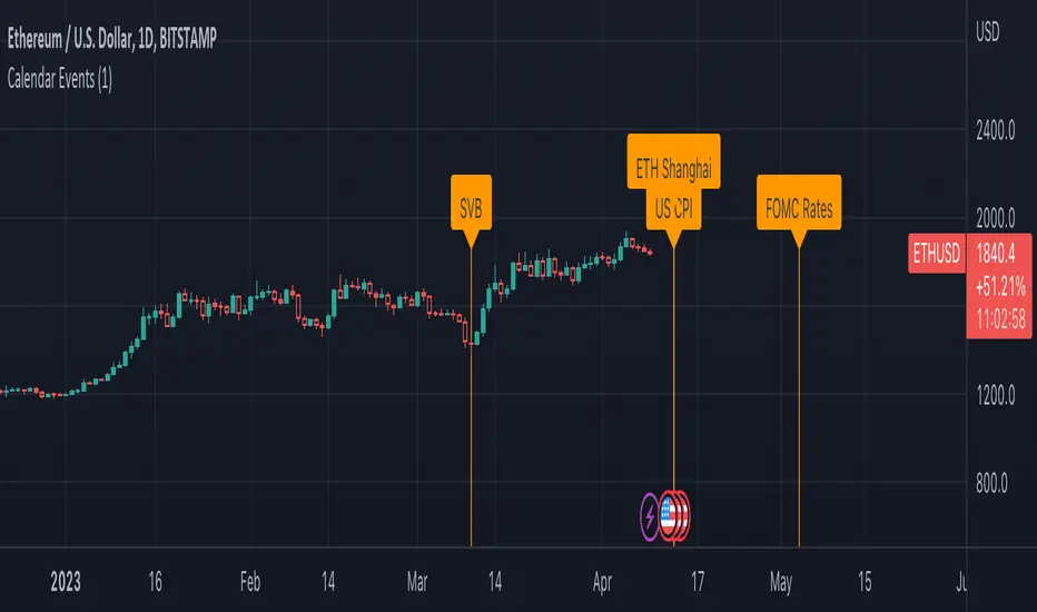
[BTX] Triple TRIX + MAsThis indicator suggest a strategy, which is quite similar to multiple MA or multiple RSI strategies.
This indicator can be used for all timeframes, all markets.
This indicator can help detect the market trend and momentum.
Default values are TRIX - 6, 12, and 24 periods and MA(8) for each TRIX line. You can choose what type of MA to be used (EMA or SMA).
How to exploit this indicator?
- When all of the lower TRIXs are ABOVE the higher one: TRIX(6) is above TRIX(12), and TRIX(12) is above TRIX(24), there is a BULLISH market.
- When all of the lower TRIXs are BELOW the higher one: TRIX(6) is below TRIX(12), and TRIX(12) is below TRIX(24), there is a BEARISH market.
- A crossover of the lower TRIX to the higher one indicates a BUY signal.
- A crossunder of the lower TRIX to the higher one indicates a SELL signal.
- TRIX crossover the Zero line can be considered as a STRONG bullish signal.
- TRIX crossunder the Zero line can be considered as a STRONG bearish signal.
- The MA of TRIX acts as a confirmation, it can be used as SELL signals.
- High slopes of TRIX lines can point out the high momentum of the current trend.
- Divergence patterns can be used with this indicator.
- And many more tricks.
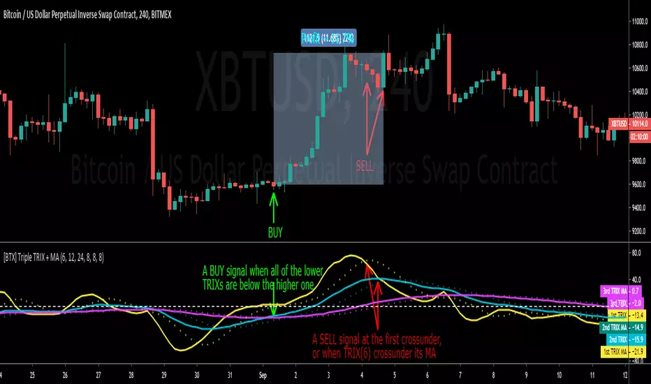
Fib,Guppy Multiple MA(FGMMA)(A/D & Volume Weight,SMA,EMA)[cI8DH]Features:
- 3 + 12 MAs (12 is chosen because Guppy has 12 MAs)
- MA types can be set to Simple, Exponential, Weighted, and Smoothed
- Volume weight can be applied to all available MAs (the built-in VWMA uses Simple MA)
- It is possible to count in only effective portions of the volume in the equation by using Accum/Dist Volume Weight
- Secondary smoothing (useful when volume weight is enabled)
- Predefined MA sets based on Fibonacci sequence (2,3,5,8,.., 377), Guppy (3,5,8,10,12,15 &30,35,40,45,50,60), and cI8DH (2,3,5,8,12,17 & 30,34,39,45,52,60)
Recommended settings:
- hlc3 as input source captures all the essential information encapsulated in a candle. I'd use hlc3 as the default option. In uptrend, "low" and in downtrend, "high" might give more relevant results when using MAs for structural analysis of a market. For commonly used MAs (EMA20, SMA50,100,200), "close" should be used due to their self-fulfilling prophecy effect.
- When you have volume weight above 0, you may want to use secondary smoothing.
- Try not to use Simple MA for smaller lengths (below 20). Sharp changes in the past (right before the period specified by the length) will affect the current value of MA dramatically leading to confusion.
- I am using the first 3 MAs for SMA 50,100,200. You can disable them from the MA type selector all at once when using Fib or Guppy ribbons.
MA-based analysis:
There are different ways of structuring a market. Geometrical (trend lines, channels, fans, patterns, etc) and Fib retracement-based structuring is very common among traders. MAs give an alternative way of analyzing markets. MA ribbons such as Guppy (6 slow and 6 fast-moving MAs) are popular for analyzing market flow. IMO default Guppy sets are a bit random as the numbers do not have an elegant sequence. So I proposed my sets based on increasing sequene spacing (+1). These two MA ribbons are good for market flow analysis but the spacing of the MAs are not ideal for structuring a market. Ribbons based on the Fib sequence is a better choice for structuring a market. This is the equivalent of Fib channels but in a more dynamic form. Among other things, MA Fib ribbon can be used to assess market momentum and to compare different stages of a market. Here are two "educational-only" examples:
Notes:
- Smoothed MA with length L = Exponential MA with length 2*L-1
- Read the background section in my ADP indicator to understand how A/D Volume is calculated

XPloRR MA-Trailing-Stop StrategyXPloRR MA-Trailing-Stop Strategy
Long term MA-Trailing-Stop strategy with Adjustable Signal Strength to beat Buy&Hold strategy
None of the strategies that I tested can beat the long term Buy&Hold strategy. That's the reason why I wrote this strategy.
Purpose: beat Buy&Hold strategy with around 10 trades. 100% capitalize sold trade into new trade.
My buy strategy is triggered by the fast buy EMA (blue) crossing over the slow buy SMA curve (orange) and the fast buy EMA has a certain up strength.
My sell strategy is triggered by either one of these conditions:
the EMA(6) of the close value is crossing under the trailing stop value (green) or
the fast sell EMA (navy) is crossing under the slow sell SMA curve (red) and the fast sell EMA has a certain down strength.
The trailing stop value (green) is set to a multiple of the ATR(15) value.
ATR(15) is the SMA(15) value of the difference between the high and low values.
The scripts shows a lot of graphical information:
The close value is shown in light-green. When the close value is lower then the buy value, the close value is shown in light-red. This way it is possible to evaluate the virtual losses during the trade.
the trailing stop value is shown in dark-green. When the sell value is lower then the buy value, the last color of the trade will be red (best viewed when zoomed)(in the example, there are 2 trades that end in gain and 2 in loss (red line at end))
the EMA and SMA values for both buy and sell signals are shown as a line
the buy and sell(close) signals are labeled in blue
How to use this strategy?
Every stock has it's own "DNA", so first thing to do is tune the right parameters to get the best strategy values voor EMA , SMA, Strength for both buy and sell and the Trailing Stop (#ATR).
Look in the strategy tester overview to optimize the values Percent Profitable and Net Profit (using the strategy settings icon, you can increase/decrease the parameters)
Then keep using these parameters for future buy/sell signals only for that particular stock.
Do the same for other stocks.
Important : optimizing these parameters is no guarantee for future winning trades!
Here are the parameters:
Fast EMA Buy: buy trigger when Fast EMA Buy crosses over the Slow SMA Buy value (use values between 10-20)
Slow SMA Buy: buy trigger when Fast EMA Buy crosses over the Slow SMA Buy value (use values between 30-100)
Minimum Buy Strength: minimum upward trend value of the Fast SMA Buy value (directional coefficient)(use values between 0-120)
Fast EMA Sell: sell trigger when Fast EMA Sell crosses under the Slow SMA Sell value (use values between 10-20)
Slow SMA Sell: sell trigger when Fast EMA Sell crosses under the Slow SMA Sell value (use values between 30-100)
Minimum Sell Strength: minimum downward trend value of the Fast SMA Sell value (directional coefficient)(use values between 0-120)
Trailing Stop (#ATR): the trailing stop value as a multiple of the ATR(15) value (use values between 2-20)
Example parameters for different stocks (Start capital: 1000, Order=100% of equity, Period 1/1/2005 to now) compared to the Buy&Hold Strategy(=do nothing):
BEKB(Bekaert): EMA-Buy=12, SMA-Buy=44, Strength-Buy=65, EMA-Sell=12, SMA-Sell=55, Strength-Sell=120, Stop#ATR=20
NetProfit: 996%, #Trades: 6, %Profitable: 83%, Buy&HoldProfit: 78%
BAR(Barco): EMA-Buy=16, SMA-Buy=80, Strength-Buy=44, EMA-Sell=12, SMA-Sell=45, Strength-Sell=82, Stop#ATR=9
NetProfit: 385%, #Trades: 7, %Profitable: 71%, Buy&HoldProfit: 55%
AAPL(Apple): EMA-Buy=12, SMA-Buy=45, Strength-Buy=40, EMA-Sell=19, SMA-Sell=45, Strength-Sell=106, Stop#ATR=8
NetProfit: 6900%, #Trades: 7, %Profitable: 71%, Buy&HoldProfit: 2938%
TNET(Telenet): EMA-Buy=12, SMA-Buy=45, Strength-Buy=27, EMA-Sell=19, SMA-Sell=45, Strength-Sell=70, Stop#ATR=14
NetProfit: 129%, #Trade

Back to zero: Understanding seriestype: pine series basic example
time required: 10 minutes
level: medium (need to know the "array" data variable as a generic programming concept, basic Pine syntax)
tl;dr how variables and series work in Pine
Pine is an array/vector language. That's something that twists how it behaves, and how we have to think about it. A lot of misunderstandings come from forgetting this fact. This example tries to clear that concept.
First, you need to know what an array is, and how it works in a programmig language. Also, having javascript under your belt helps too. If you don't, google "javascript array basic tutorial" is your friend :)
So, in pine arrays are called "series". Every variable is an array with values for each candle in the chart. if we do:
myVar = true
this is not a constant. It is a series of values for each candle, { true, true,....., true }
In practice, the result is the same, but we can access each of the values in the series, like myVar{0}, myVar{7}, myVar{anyNumber}....
Again, it is not a constant, since you can access/modify the each value individually
so, lets show it:
plot (myVar, clolor = gray)
this plots an horizontal line of value 1 ( 1 is equal to true ) so it's all good.
On to a more usual series:
tipicalSeries = close > open ? true : false
plot(tipicalSeries, color= blue)
This gives the expected result, a tipical up and down line with values at 1 or 0. Naturally, "tipicalSeries" is an array, the "ups" and "downs" are all stored under the same variable, indexed by the candles.
In Pine, the ZERO position in the array is the last one, which corresponds to the last candle on the right. Say you have a chart with 12 candles. The close would be the closing value of what we intuitively think as first candle, the one on the left. then close ... and so on.... until close , the value of the "last" candle, the one on the right. It actually helps to start thinking of the positions backwards, counting down to zero, rocket launch style :)
And back to our series. The myVar will also be the same size, from myVar to myVar .
When we do some operation with them, something simple like
if ( myVar == tipicalSeries)
what is really happening is that internally, Pine is checking each of the indexes, as in myVar == tipicalSeries , myVar == tipicalSeries .... myVar == tipicalSeries
And we can store that stuff to check it. simply:
result = (myVar == tipicalSeries) ? true : false //yes, this is the same as tipicalSeries, but we're not in a boolean logic tut ;)
plot (result)
The reason we can plot the result is that it is an array, not a single value. The example indicator i provide shows a plot where the values are obtained from different places in the array, this line here:
mySeries3 = mySeries2 and mySeries1
this creates a series that is the result of the PREVIOUS values stored (the zero index is the one most at the right, or the "current" one), which here just causes a shift in the plotted line by one candle.
Go ahead, grab a copy of my code, try to change the indexes and see the results. Understanding this stuff is critical to go deeper into Pine :)
