MTF Bullish/Bearish IndicatorThe script plots a bullish/bearish indicator by evaluating a variety of moving averages for a security across multiple timeframes. It's derived from built in Technical Analysis indicator published by TradingView. The result of evaluation is plotted on the chart in green light/red light format in a configurable location.
evaluated moving averages include
- SMA 10, 20, 30, 50, 100, 200
- EMA 10, 20, 30, 50, 100, 200
- Hull MA 9
- VWMA 20
- Ichimoku Cloud
moving averages are evaluated at chart timeframes and 5 min, 15 min, 30 min, 120 min, 240 min, and daily by default but can be customized.
Cari dalam skrip untuk "20日线角度大于0的股票"
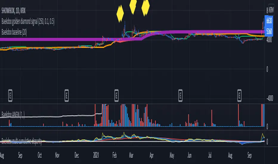
Baekdoo baselineHi forks,
I'm trader Baekdoosan who trading Equity from South Korea. This Baekdoo baseline will give you the idea of big whale's approximate average price. The idea behind this indicator is to combine volume and price. Here's one of the equation.
...
HT4=highest(volume, 250)
NewH4=valuewhen(volume>HT4 , (open+close+low+high+close)/5, 1)
result4=ema(NewH4, 20)
...
As you can see it will update when highest volume is updated by certain period of time. At that update will be the price of the close weighted price. and I put shift value of 20 (offset of input value) due to putting time theorem of Ichimoku Balance Table. 20 days means for 1 month of market day.
Why this idea work? It is mainly for the support / resistance. Resistance is made for lots of individual's buy. When the price goes down, they are tend to hold. As time goes by price getting high to their average price, then they are selling it with small profit or the same price or with small loss. So resistance is made by lots of individuals. And supports are made by small number of big whales. If we see the volume only, then we cannot differentiate easily for lots of individuals and small number of big whales. But lower price's large volume will most probably be the whale where higher price's large volume will most probably tons of individuals.
hope this will help your trading on equity as well as crypto. I didn't try it on futures. Best of luck all of you. Gazua~!
Multi-Length Stochastic Average [LuxAlgo]This indicator returns the average of stochastic oscillators with periods ranging from 4 to length . This allows for a slightly more reactive oscillator as well as having information regarding the position of the price relative to rolling maximums/minimums of different periods.
We introduce settings that allow for pre and post-smoothing, with selectable smoothing methods and periods for both steps.
Settings
Length: Period of the indicator, determine the maximum period of the stochastic oscillator used in the average
Source: Source input of the indicator
Pre-Smoothing (1st Input): Degree of smoothing applied to the source input
Pre-Smoothing (2nd Input): Pre-Smoothing Method
Post-Smoothing (1st Input): Degree of smoothing applied to the final oscillator output
Post-Smoothing (2nd Input): Post-Smoothing Method
Smoothing methods include a simple moving average, a triangular moving average, and a least-squares moving average (this method can induce overshoots during the post-smoothing step). The user can also select "None".
Usages
The "multi-length" aspect of technical indicators is something that hasn't been deeply explored yet such indicators can give us information regarding both short-term and long-term information which was the motivation for the creation of the indicator.
The Multi-length Stochastic Average allows us to quantify the price position relative to a multitude of highest/lowest levels.
In the example above the oscillator returns the average of stochastic oscillators with periods ranging from 4 to 20, as well as multiple rolling minimums with periods ranging from 4 to 20. We can see that when the price is equal to all rolling minimums the oscillator is equal to 0, the oscillator would return 100 if the price were equal to all rolling maximums with periods in that same range.
The oscillator can be interpreted like any scaled oscillator and can be used to estimate trend direction as well as trend strength.
Here we only make of use pre-smoothing by using a period 20 simple moving average. The indicator graphical elements such as colors/circles can help us determine potential directions trends might take.
Circles are displayed when the oscillator crosses over/under the 20/80 level. Such conditions offer better timing than waiting for the oscillator to be greater/lower than 50 and are less subjective to noise than simply looking at the direction taken by the oscillator. However, it can suffer from potential retracements in a trend more easily, this is illustrated in the chart above.

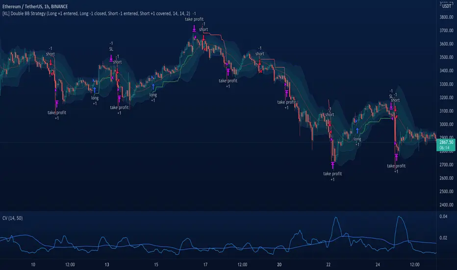
[KL] Double Bollinger Bands Strategy (for Crypto/FOREX)This strategy uses a setup consisting of two Bollinger Bands based on the 20 period 20-SMA +/-
(a) upper/lower bands of two standard deviations apart, and
(b) upper/lower bands of one standard deviation apart.
We consider price at +/- one standard deviation apart from 20-SMA as the "Neutral Zone".
If price closes above Neutral Zone after a period of consolidation, then it's an opportunity for entry. Strategy will long, anticipating for breakout.
The illustration below shows price closing above the Neutral Zone after a period of consolidation.
a.c-dn.net
Position is exited when prices closes at Neutral Zone (being lower than prior bars)
Optimized Keltner Channels SL/TP Strategy for BTCThis strategy is optimized for Bitcoin with the Keltner Channel Strategy, which is TradingView's built-in strategy. In the original Keltner Channel Strategy, it was difficult to predict the timing of entry because the Buy and Sell signals floated in the middle of the candle in real time. This strategy is convenient because if the bitcoin price hits the top or bottom of the Keltner Channel and closes the closing price, you can enter Buy or Sell at the next candle start price. In addition, this strategy provides Stop Loss and Take Profit functions to maximize profit.
_________________________________
Recommended settings are below.
- length: 9
- multiplier: 1
- source: close
- (v) Use EMA
- Bands Style: Average True Range
- ATR Length: 19
- Stop Loss (%): 20
- Take Profit (%) : 20
_________________________________
- length: 9
- multiplier: 1
- source: close
- (v) Use EMA
- Bands Style: Average True Range
- ATR Length: 18
- Stop Loss (%): 20
- Take Profit (%) : 5
_________________________________
▶ Usefulness and Originality
- Stop Loss and Take Profit functions are available
- Convenient Buy and Sell entry compared to the original Keltner Channel Strategy
- Optimized for BTCUSD market (maximizing profits)
___________________________________________
이 전략은 TradingView의 Built-in 전략인 Keltner Channel Strategy를 비트코인에 맞게 최적화되었습니다. 기존의 Keltner Channel Strategy는 Buy, Sell 신호가 캔들 중간에 실시간으로 떠서 진입 시점을 예측하기 어려운 불편함이 있었지만 이 전략은 비트코인 가격이 Keltner Channel 상단 혹은 하단을 찍고 종가를 마감하면 그 다음 캔들 시작가에서 Buy 혹은 Sell 진입이 가능하여 편리합니다. 또한, 이 전략은 Keltner Channel을 만나서 캔들을 마감한 가격 (bprice, sprice)을 시각적으로 plot을 제공하여 타점 및 차트를 보기에 편리하며 손절가 및 목표가를 지정한 백테스팅이 가능합니다.

[KBCUSTOM] Histogramified Stochastic RSI The public and regular stoch RSI does not come with a histogram which makes it hard to tell the magnitude of any cross. This version comes with one enabled by default and with includes buy and sell triggers on specified crosses.
Buy & Sell Options:
KB Cross Factor: this is the minimum stochastic change between candles that needs to be exceeded in order to trigger a buy or sell signal. For instance, if the previous candle has a value of -20, and the next one has 10, then the factor should be 30 in order for it to trigger a signal.
KB Cross Threshold: in order to minimize bad signals due to weak trend, you can set the minimum stochastic value any candle should have for an order signal to trigger. For instance, say the stochastic has a good cross factor (i.e. 30) and is met, and the stochastic has a value of 10 but your cross threshold is set at 20, then the signal will not trigger unless it is actually 20 or higher.
Let me know how it works.
Cheers.

Drawdown RangeHello death eaters, presenting a unique script which can be used for fundamental analysis or mean reversion based trades.
Process of deriving this table is as below:
Find out ATH for given day
Calculate the drawdown from ATH for the day and drawdown percentage
Based on the drawdown percentage, increment the count of basket which is based on input iNumber of ranges . For example, if number of ranges is 5, then there will be 5 baskets. First basket will fit drawdown percentage 0-20% and each subsequent ones will accommodate next 20% range.
Repeat the process from start to last bar. Once done, table will plot how much percentage of days belong to which basket.
For example, from the below chart of NASDAQ:AAPL
We can deduce following,
Historically stock has traded within 1% drawdown from ATH for 6.59% of time. This is the max amount of time stock has stayed in specific range of drawdown from ATH.
Stock has traded at the drawdown range of 82-83% from ATH for 0.17% of time. This is the least amount of time the stock has stayed in specific range of drawdown from ATH.
At present, stock is trading 2-3% below ATH and this has happened for about 2.46% of total days in trade
Maximum drawdown the stock has suffered is 83%
Lets take another example of NASDAQ:TSLA
Stock is trading at 21-22% below ATH. But, historically the max drawdown range where stock has traded is within 0-1%. Now, if we make this range to show 20 divisions instead of 100, it will look something like this:
Table suggests that stock is trading about 20-25% below ATH - which is right. But, table also suggests that stock has spent most number of days within this drawdown range when we divide it by 20 baskets instad of 100. I would probably wait for price to break out of this range before going long or short. At present, it seems a stage ranging stage. I might think about selling PUTs or covered CALLs outside this range.
Similarly, if you look at AMEX:SPY , 36% of the time, price has stayed within 5% from ATH - makes it a compelling bull case!!
NYSE:BABA is trading at 50-55% below ATH - which is the most it has retraced so far. In general, it is used to be within 15-20% from ATH
NOW, Bit of explanation on input options.
Number of Ranges : Says how many baskets the drawdown map needs to be divided into.
Reference : You can take ATH as reference or chose a time window between which the highest need to be considered for drawdown. This can be useful for megacaps which has gone beyond initial phase of uncertainity. There is no point looking at 80% drawdown AAPL had during 1990s. More approriate to look at it post 2000s where it started making higher impact and growth.
Cumulative Percentage : When this is unchecked, percentage division shows 0-nth percentage instad of percentage ranges. For example this is how it looks on SPY:
We can see that SPY has remained within 6% from ATH for more than 50% of the time.
Hope this is helpful. Happy trading :)
PS: this can be used in conjunction with Drawdown-Price-vs-Fundamentals to pick value stocks at discounted price while also keeping an eye on range tendencies of it.
Thanks to @mattX5 for the ideas and discussion today :)

[VJ] Hulk Smash IntraThis is a simple intraday strategy for working on Stocks or commodities based out on Super Trend and ever reliable ADX . You can modify the start time and end time based on your timezones. Session value should be from market start to the time you want to square-off
Important: The end time should be at least 2 minutes before the intraday square-off time set by your broker
Comment below if you get good returns
Strategy: Supertrend and ADX strength (Hulk Smash)
Indicators used :
Super trend is simple and easy to use indicator and gives a precise reading about an on going trend.It is built with two parameters, namely period and multiplier.The Buy and Sell signal modifies once the indicator tosses over the closing price. When the Super trend closes above the Price, a Buy signal is generated, and when the Super trend closes below the Price, a Sell signal is generated. In this case we use it only for direction .
ADX informs a trader when the market is trending.It filters out anti trend trades to help trend chasing indicators from frequent whipsaws
Multiplier is a vital input for Super trend. If the multiplier value is too high, then lesser number of signals is made.
Buying/Selling
• If the price is going UP, and the ADX indicator is also going UP, then we have the case for a bullish trend.
• The same is true if the price is going down and the ADX indicator is going UP. Then we have the case for a bearish trend.
• Value of ADX below 20 is called trading zone which implies non-trending market
• Trade with Strength only if the Super trend is validating
ADX Values
0 - 20 : Non Trending (Range bound market, phase of Accumulation/Distribution)
20-45 : Strong Signal (helpful for traders)
45-60 : Very strong trend (occur rarely, indicate exhaustion)
60 - 100 : Extremely strong trend (very rare, unsustainable trends, be ready for reversals)
Usage & Best setting :
Choose a good volatile stock and a time frame - 5m.
ADX Factor : vary as per info above
ST multiplier : 3
There is stop loss and take profit that can be used to optimise your trade
The template also includes daily square off based on your time.

Rolling ReturnsWhat does this indicator show?
This indicator shows the rolling return of a set lookback period.
The default indicator value is 20 which will show the rolling 20-day return because 20 trading days is 1 month.

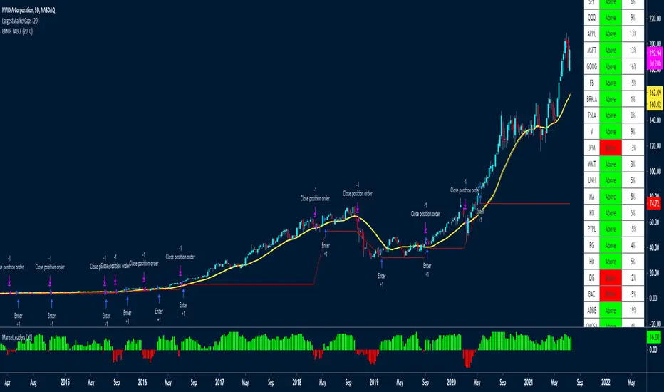
LargestMarketCapsThis trading system uses a MA to check if the LARGEST CAP stocks are above or below the MA.
You can see from the indicator below how well it manages to capture big moves.
It aggregates the data of all the tickers to create the histogram indicator at the bottom of the chart called MarketLeaders.
If a ticker is above its moving average, then the output will increase by +1 and -1 if a ticker is below its moving average.
This is a powerful system because it uses not only data from one stock but from the stocks that really affect the market big time. If those stocks don't do well, the market won't do well either.
Basically if all the market leaders are doing well, then this system will buy those 20 tickers and keep positions open until the MarketLeaders indicator crosses below 0 -- meaning red.
It also has a red stop loss line, with a wide 15% stop loss to keep us in the trades for the long term.
I've used a 5-day chart because I wanted fewer signals, but higher quality signals.
There are no profit targets, this exits when the indicator turns red -- meaning below 0 or if a position falls 15% in price.
The MA setting is adjustable, the default is 20
These are the tickers that the strategy and indicator currently looks at
The tickers will need to be updated every 6-12 months to remove and ad those who have dropped out of the largest 20 stocks.
It would be a good idea to create a watchlist and alerts for the Large Cap tickers so you can scroll through to see how the system performed on each ticker
"SPX"
"QQQ"
"AAPL"
"MSFT"
"GOOG"
"FB"
"BRK.A"
"TSLA"
"V"
"JPM"
"WMT"
"UNH"
"MA"
"KO"
"PYPL"
"PG"
"HD"
"DIS"
"BAC"
"ADBE"
"CMCSA"
"NKE"
RELATED IDEAS / Indicators
Market Leaders Ribbon
Market Leaders Large Performance Table
RedK Volume-Weighted Directional Efficiency Index (DXF)RedK Volume-Weighted Directional Efficiency Index (DXF) is a momentum indicator - that builds on Kaufman's Efficiency Ratio (ER) concept.
DXF utilizes a restricted +100/-100 oscillator to represent the "quality" of a trend, and does a good job in detecting the possibility of an upcoming trend change (in both direction and quality), improving our ability to make decisions on trade entries and exits.
Here's a quick background on Kaufman's Efficiency Ratio (ER)
------------------------------------------------------------------------------- Copied from internet sources -----------------------------
Developed by Perry Kaufman and introduced in his book “New Trading Systems and Methods”, the Efficiency Ratio reflects relative market speed to volatility. There are cases, when it is used as a filter, which helps a trader to avoid ”choppy” markets or trading ranges and to identify smoother trends.
ER is the result of dividing the net change in price movement during n-periods by the sum of all bar-to-bar price changes during the same n-periods. In case the market is trending smoother, then the ratio will be higher. In case the ratio shows readings in proximity to zero, this implies that market movement is inefficient and ”choppy”.
If the Efficiency Ratio shows a reading of +100, this means that the trading instrument is in a bull trend and trending with perfect efficiency.
If the Efficiency Ratio shows a reading of -100, this means that the trading instrument is in a bear trend and trending with perfect efficiency.
It is impossible for any instrument to have a perfect Efficiency ratio, because any movement against the major trend during the examined period of time would cause the ratio to drop.
If the Efficiency Ratio shows a reading above +30 (common setting for the "Significant Level"), this is indicative of a quality bull trend. If the ratio shows a reading below -30, this is indicative of a quality bear trend.
------------------------------------------------------------------------------- End of Copy -------------------------------------------------------------------------------------------------------
Kaufman also used the ER as basis for his famous Kaufman Adaptive Moving Average (KAMA).
Read more on ER & Kama here
How is DXF different from other ER-based indicators?
------------------------------------------------------------------
- Let's get the easy part out of the way: DXF has a "volume-weighting" option ✔
This option is OFF by default (to avoid errors with instruments with no volume data)
- once this option is applied, it provides the benefit of combining the volume effect into the calculation - those who appreciate the effect of volume on price action will hopefully find this option valuable
- The calculation of ER and how it can be "best utilized":
Let's examine the ER concept a bit closer: as a (math) concept, the (original) Efficiency Ratio (ER) takes the positive change of the price of an instrument during a certain period, and divide it by the sum of (absolute) price moves that were observed during that same period.
So, in the trader's language, we will be saying "out of a total of $20 moves (up and down) that MSFT did in the past 10 days, MSFT only made a net change of $5 up during that period" - so the "10-day ER" for MSFT in that case is 5/20 = 25% -- then we continue to observe that ongoing "10-day ER" and if it increases, we can expect that MSFT is going to establish a strong move (trend) up --- right?
the magic word here is to "observe the ongoing ER" - many of the ER based indicators just use the ER as calculated by Kaufman's original method. IMHO, these are just "point-in-time readings" - if we hope to get real insights from the ER, we need to take an average of that reading - for our "time window" we're interested in - and only then we can identify trends and patterns in the ER value as it changes during that windowss- DXF does that - and that allows a trader to say "the (weighted) 5-day average of the 10-day ER for MSFT is increasing, and that why i expect an up-trend" -- makes sense ? both the "Lookback" used to calculate the ER, and the Length of observed "window" for the Average ER are adjustable in DXF settings
Other Uses and Settings :
---------------------------------
- As a momentum indicator, DXF can predict an upcoming change of trend - cause that will reflect on the average ER value. There are few examples in the chart where the price move and ER trend *do not agree* - The trader can see these signs and take decisions accordingly
- DXF can help reveal best entries and exits: assume we are long-term bullish on MSFT, and we want to "buy the dip" - DXF can help reveal the time where price is recovering from extreme weakness - and that would be the ideal buy opportunities for us - exampled marked on the chart
- the Stepping & Smoothing options enable better visualization of the DXF plot. the "raw" DXF is still shown as a silver line.
- The "Significant Levels" option is available and is set to -20/+20 by default .. also adjustable in indicator settings.
- Please use DXF in combination with other trend and volume indicators, and with thorough chart / price action analysis and not in isolation to ensure you get proper signal confirmation for trades. In the chart above, you can see DXF combined with a moving average that can act as a filter and to confirm the price moves.
---------------------------------------------------
As usual, feedback & comments are welcome - if you find this work useful in your trading arsenal, please share a comment - i would be more than happy to learn about that. Good luck!

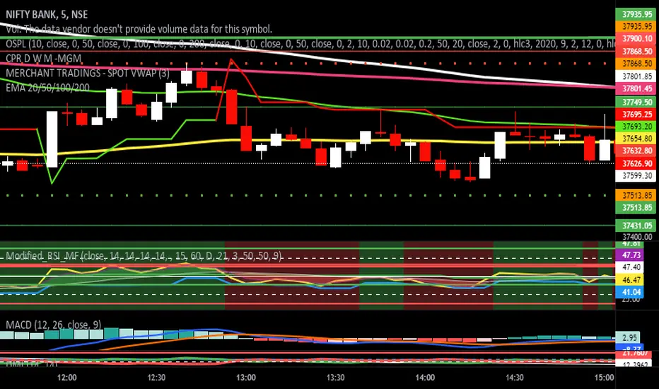
Modified RSI Multi-Time Frame (HM)Effective RSI with Multi-Timeframe with Hilema - Milega(HM) concept (HM=WMA -EMA). RSI Script is included with WMA and EMA band for RSI1 and it works very simple
i) When the RSI band turns to Green its a Buy signal. Normally whenever Bearish strength weakens and move towards the Bullish area, the WMA and EMA cross each other and that tends to provide a possible trend change. A trade at crossover normally provides a very good trading oppertunity. One can combine with some other Price action if needed for double confirmation.
ii)When RSI band turns to RED its a Sell signal. As explained in the point 1 , its a vice-versa where a crossover of WMA and EMA is perfect entry to get a good swing trade. Once can combine this tool with Price action for double confirmation.
iii) Using the Multi timeframe user could able to find the trend at higher timeframe to take double confirm on the trend strength and take a perfect oppertunity to take the trade.
By default, script uses the RSI with length 14, WMA 21 and EMA 3 which perfectly working for Index in NSE. Please change as per your requirement.
Apart from the above band, RSI is not have the different levels like 20/ 40 /50/60/80
Multi-timeframes currently set as
RSI1 - Same as Chart
RSI2 - 15 Min
RSI3 - 60 Min
RSI4 - Daily
Script has enabled the option to change the values for these timeframes as per the user requirement.
These ranges can be interpreted and acts as a probable swing points based on the trend and momentum.
40-60 - Neutral Range or Sideways
20 - 60 Bearish range
40 - 70 - Bullish range
Below 20 -- Over Sold Zone
Above 80 - over Bought zone
Also, the crossovers of the WMA and EMA on the RSI gives a very good momentum towards that trend.
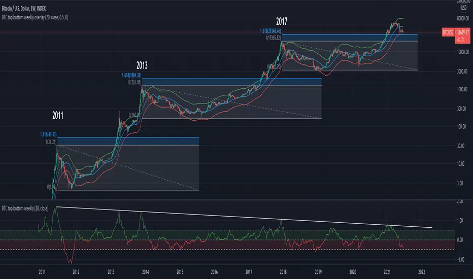
BTC top bottom weekly oscillatorThis indicator is based on the 20 weekly simple moving average and it could be used to help finding potential tops and bottoms on a weekly BTC chart.
This version uses an "oscillator" presentation, it fluctuates around the value zero.
The indicator plots 0 when the close price is near the 20 weekly moving average.
If it's below 0 it reflects the price being below the 20 weekly moving average, and opposite for above.
IT's possible to see how many times the price has hit the 0.5 coef support. In one case it hit 0.6 showing that the 0.5 support can be broken.
The indicator is calculated as Log(close / sma(close))
Instructions:
- Use with the symbol INDEX:BTCUSD so you can see the price since 2010
- Set the timeframe to weekly
Optionals:
- change the coef to 0.6 for a more conservative bottom
- change the coef to 0.4 for a more conservative top
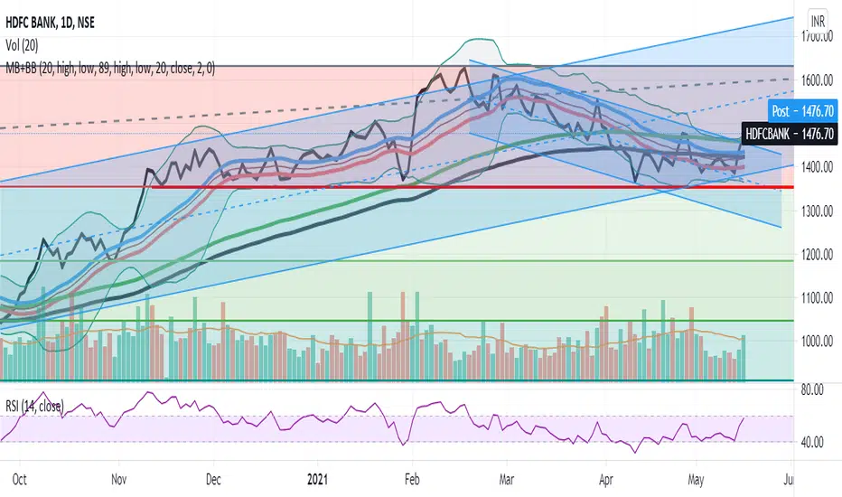
Magic BandBSE:DLF
I have integrated Moving average, Bollinger bands and Exponential moving average. It has two SMA,
The first thing is 20 SMA with blue coloured SMA line source as high and red coloured SMA line source as low, this together forms a band which can be used for a swing trade, usually useful in bull run of the stock and price tries to get support on this band.
the second thing in this is similar to the previous set up but it plots 89 period EMA, this becomes useful in the smaller timeframe when one step larger timeframe is near to 20 SMA band
the third thing is plots of Bollinger band with 20 SMA, which gives us an idea on volatility.
McClellan Oscillator for nifty 50This is a indicator which indicates breath of the market.
If found relevant do let me know!!
Only handpicked relevant 20 stocks (20 +ve indicator+ 20 -ve indicator) from different sector .
As there is the limit of 40 script allowed only.
Further modifications might be there if the limit is increased to 100 (50 +50 indicator) .

A simple double moving average system# This simple code is describing the double moving average system, thanks for the contribution of Lei and jchang264
# The moving average system is including the SMA(20,60,120) and EMA(20,60,120), which use the different colours and style
# The bar is using the different colours to describe the different state, for example the black one mean the season of the trendy didn't form, the blue mean to reach the first phase of the trendy, the state of gray bar just between the black and blue, The gold one mean the season of the trend has already forming (SMA20 > SMA60 > SMA120), which one I think it is important.
# Price mark mean the deduction price of 20, 60 and 120

Price Action IndexI've created a simple oscillator which I think does a good job of easily showing you when price is worth watching or not. I think all too often you get stuck looking at something like an RSI and end up trading noise.
From my observations and experiences, I've found that there are 2 major catalysts for price movement--
Price is either trending and reaches a top or bottom, or
Price is consolidating and ready to make a move in some direction
These movements can be seen quite well from a Bollinger Band, which is what mostly gave me the inspiration. When I watch a chart with a BB on it I see that either you're looking to trade price moving out of a squeeze or riding price up/down the band until it crosses over and makes a move to the moving average.
My solution was to multiply the direction of price by the strength of its deviation.
Price gets converted into a signal between -1.0 (bottom of the range) and 1.0 (top of the range)
Standard Deviation gets converted into a stochastic signal between 0 (next to no deviation from mean) and 100 (highest deviation in lookback)
These 2 get multiplied by each other
The result tells you if price action is trending bullish and if its approaching max strength (perhaps Overbought), example: Price is hitting highs (1.0) and deviation is also at its highest (100) = 100, opposite for bearish
Result can also tell you if price is at the top of the range but the deviation is so tiny and we're mostly pinned to the mean (1.0 * 5 = only 5)
How to Trade this Indicator--
If the indicator is stuck near the middle and purple:
- Don't make directional trades or you'll be eaten alive by the chop
- Good idea to sell options, Iron Condors/Butterflies, etc
- Wait for a move to breakout --> the purple will fade away and give way to a direction
--- As in all trading scenarios, be mindful of fakeouts/short moves to one direction that very quickly get reversed
If the indicator is heading higher:
- This would indicate there is a bull trend going on, get long
- If we are reaching the overbought area, this is an ideal place to take profits or look at spreads like Bearish Call Spreads (sell calls)
- I think you can make your own determination of when to sell by either selling when we're in the overbought area (if it reaches there) or staying bullish so long as it is above the zone
If the indicator is heading lower:
- Bear trend, shorting is possible
- Can use this as a contrarian signal to buy lows
A couple of charts with the indicator and a purple squeeze box I've drawn (can sometimes get noisy in real-time, but hindsight is 20/20)--
Bitcoin on Daily with default 20 length
Gamestop on 30 minute time frame with 100 length
Please feel free to use this indicator for your trading or your own indicators. This particular script is very stripped down/bare bones from what I have been working on as an ongoing project. If TradingView ever returns scripts you can sell, I would probably open that up for a small premium.

Rainbow Trend IndicatorThis is an indicator based on the MA rainbow concept. It is possible to choose between 15 or 20 MA's and if all 15 MA's is picked, the calculation will be calculated on 15 MA's and if 20 is picked the calculation is calculated on 20 MA's. The indicator will then be a line which is assigned a value from the calculation based on the MA's. If the line is above the dashed zero line, meaning the line's last value is a positive value, the price is in a uptrend and if the line is below the dashed zero line, meaning the line's last value is a negative value, the price is in a downtrend.
In short
If the line is green, the price is in a uptrend. If the line is red, the price is in a downtrend.

Koalafied RSI// Concept developed from RSI : The Complete Guide by John Hayden
// RSI is regarded as a momentum indicator. 2:1 momentum is associated with RSI values of 66.67 and 33.33 respectfully. In an Uptrend an RSI value of 40 should not be broken and in a downtrend
// a RSI value of 60 should not be exceeded. 4:1 momentum (RSI values of 80/20) can be associated with extreme market conditions, typically thought of as being Overbought or Oversold.
// Simple divergence provides a strong indication that the preceding trend will resume as soon as the retracement is completed. Multiple long-term divergences (not shown in this indicator)
// increase the likelihood that the preceding trend has ended.
// An Uptrend is indicated when:
// 1. RSI values remain in an 80/40 range
// 2. Presence of bearish divergences
// 3. Hidden bullish divergences are seen
// A Downtrend is indicated when:
// 1. RSI values remain in a 60/20 range
// 2. Presence of bullish divergence
// 3. Hidden bearish divergence is seen
// Personal additions to John Haydens concepts are horizontal pivot breaks and diagonal trendline breaks. The 80/20 line color shows the last break of horizontal pivot points, while the rsi
// line changes color with diagonal breaks. Additional support/resistance is shown by 66.67 and 33.33 lines.

Market Traffic LightThis indicator visualizes warning and panic signs, which are shown separately.
1. Section (Fear & Greed)
Approximation of the CNN Money Fear & Greed index based on code of user MagicEins. The index shows values between 0 (extreme fear, red) and 100 (extreme greed, green).
2. Section (warning signs)
VIX: Values above 20 are red and below green. The legend shows the value of the current bar including the change from the bar before. The average VIX is about 16. Values over 20 are a sign of stressed market.
Distribution days: A distribution day (loss to the day before > 0,2 % and higher volume) is marked with a yellow dot. In case there are more than four distributions days within 25 markets days the dot is orange. When big players redistribute their investments distribution days can occur. If this is done often (more than four times within 25 market days) it is possible that the markets changes or that a sector rotation occurs. For calculation distribution days futures of S&P 500 (ES1!) and NASDAQ (NQ1!) are used because the volume for this calculation is needed. TradingView does not support volumes for S&P 500 or NASDAQ directly.
Markets: A green/red dot signals that the market is above/below its 25-Daily-EMA. A green/red square signals that the market is above/below its 25-Weekly-EMA. Markets can give as a feeling about where investors store their money. E.g. when markets are falling but DUX (Down Jones Utility Average) is rising this means that investors put their money into save haven. This can be a sign that the markets will fall more.
3. Section (panic signs, = signs of reaching a low within a correction of a crash)
VIX-Reversion: A VIX reversion day (VIX > 20 & VIX high > VIX high of the day before & VIX high – VIX close > 3) is marked as a yellow dot
VVIX: A value equal or above 140 is marked with a yellow dot and shows absolute panic.
PCR Intra max: A value equal or above 1.4 is marked with a yellow dot.
New high/lows: New highs/lows are shown for AMEX, NYSE and NASDAQ. A yellow dot is shown if the ratio is less or equal than 0.01.
Down-Day: Down days are shown for AMEX, NYSE and NASDA. A yellow dot is shown if at least 90 % of the whole volume (up and down) is a down volume.
In Addition to the warning signs in the second section a check of the Advance Decline Line (NYSE and NASDAQ) for bullish and bearish divergences is useful. The whole set-up can be seen in the screenshot.
Only one signal normally does not give us a good prediction. Therefore we need to see these indication as a bundle. TradingView gives us the opportunity to check some striking market situations in the past. So feel free to test this indication for building up your own opinion.
Please feel free to comment in case of failures, improvements or experiences (good or bad).

MACD Trend CandlesThe script combines 2 indicators (MACD and Stoch-RSI) and puts them visually directly on the candles - can be used with normal OHLC candles or Heiken Ashi candles. Furthermore, you can derive divergences exremely easy directly visually from the candles as well. Lastly, a SMA 20 high and a SMA 20 low line build a trend channel.
Script is best used in trending markets to trade with the trend.
1) SMA trend channel:
* uptrend: close above
* downtrend: close below
* aggressive entry (uptrend) closing inside channel from below
* conservative entry (uptrend) closing above channel from inside
* hold (uptrend) until close below channel
* can be used accordingly for the downtrend
2) MACD candles
* visualization of the MACD histogram directly on the candles
* dark blue: histogram > 0 and histogram > histogram of previous candle
* light blue: histogram > 0 and histogram < histogram of previous candle
* orange: histogram < 0 and histogram < histogram of previous candle
* light blue: histogram < 0 and histogram > histogram of previous candle
* hold uptrend (dark/light blue candles) - combined with trend channel (above channel)
* hold downtrend (orange /yellow candles) - combined with trend channel (below channel)
* Color divergence: light blue candle > dark blue candle (price and MACD show divergence (bearish)
* Color divergence: yellow candle < orange candle (price and MACD show divergence (bullish)
* Trend change (0 line cross to upside) yellow or orange to dark blue
* Trend change (0 line cross to downside) dark or light blue to orange
3) Stoch RSI diamonds
* visualization of the STOCH-RSI as diamonds above or below the candle
* k, d line > 80: diamond above the candle
* k, d line < 20: diamond below the candle
* divergence caldle without diamond above > candle with diamond above (bearish divergence)
* divergence caldle without diamond below < candle with diamond below (bullish divergence)
Feel free to test each part individually and combine it with other indicators, e.g. BBands and Ichimoku Cloud - you will see it is a powerful visualization script
HAVE FUN

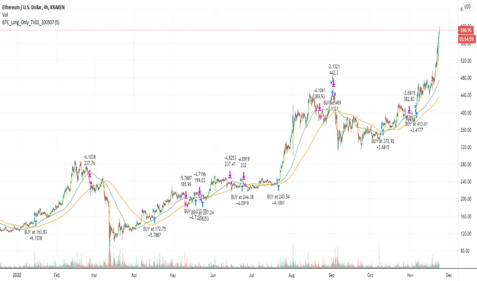
BTC and ETH Long strategy - version 2I wrote my first article in May 2020. See below
BTC and ETH Long strategy - version1
After 6 months, it is now time to check the result of my script for the last 6 months.
XBTUSD (4H): 14/05/2020 --> 22/11/2020 = +78% in 4 trades
ETHXBT (4H): 14/05/2020 --> 22/11/2020 = +21% in 9 trades
ETHUSD (4H): 14/05/2020 --> 22/11/2020 = +90% in 6 trades
Using the signals from this strategy to trade manually has shown that this was a bit frustrating because of the low rate of winning trades.
If you have to enter 100 trades and see 75% of them failing and 25% winning, this is frustrating. For sure the strategy makes good money but it is difficult to hold this mentality.
So, I have reviewed and modified it to get a higher winning rate.
After few days of work, tests and validation, I managed to get a wining rate close to 60%.
The key element was also to decrease the number of trades by using a higher time frame. (4H candles instead of 2H candles).
- Entry in position is based on
MACD, EMA (20), SMA (100), SMA (200) moving up
AND EMA (20) > SMA (100)
AND SMA (100) > SMA (200)
- Exit the position if: Stoploss is reached OR EMA (20) crossUnder SMA (100)
The goal of this new script is to be able to follow the signals manually and only make few trades per years.
I have also validated it against some other altcoins where some are giving very good results.
Here are some results for 2020 (from 01/01/2020 until now (22/11/2020). Those results are the one I get when using 4H candles.
ETH/USD: +144% in 8 trades.
BTC/USD: +120% in 7 trades.
ETH/BTC: +33% in 9 trades.
ICX/USD: +123% in 10 trades.
LINK/USD: +155% in 11 trades.
MLN/USD: +388% in 8 trades.
ADA/USD: +180% in 7 trades.
LINK/BTC: +97% in 10 trades.
The best is that above results are without considering compound effect. If you re-invest all gains done in each new trade, this will give you the below results :)
ETH/USD: +189% in 8 trades.
BTC/USD: +260% in 7 trades.
ETH/BTC: +29% in 9 trades.
ICX/USD: +112% in 10 trades.
LINK/USD: +222% in 11 trades.
MLN/USD: +793% in 8 trades.
ADA/USD: +319% in 7 trades.
LINK/BTC: +103% in 10 trades.
As you can see, the results are good and the number of trades for 11 months is not big, which allows the trader to place orders manually.
But still, I'm lazy :), so, I have also coded this strategy in HaasScript language which allows you to automate this strategy using the HaasOnline software specialized in automated crypto trading.
I hope that this strategy will give you ideas or will be the starting point for your own strategy.
Let me know if you need more details.
CCI-RSI MR Indicators:
Bollinger Bands (20 period, 2σ)
RSI (14 period) and Simple moving average of RSI (5 period)
CCI (20 period)
SMA (5 period)
Entry Conditions:
Buy when:
Swing low (5) should be lower than the highest of lower BB (3 periods)
Both RSI crossover RSI_5 and CCI crossover -100 should have happened within last 3 candles (including the current candle)
Once all the above conditions are met, the close should be higher than SMA (5) within the next 3 candles
After condition 3 is satisfied, we enter the trade at next candle’s open
Stop loss will be at 1 tick lower than previous swing low
Sell when:
Swing high (5) should be higher than the lowest of upper BB (3 periods)
Both RSI crossunder RSI_5 and CCI crossunder 100 should have happened within last 3 candles (including the current candle)
Once all the above conditions are met, the close should be lower than SMA (5) within the next 3 candles
After condition 3 is satisfied, we enter the trade at next candle’s open
Stop loss will be at 1 tick higher than previous swing high
Exit Conditions:
Since it’s mean reversion strategy we’ll be having only 2 target exits with a trailing stop loss after target price 1 is achieved.
Target exit price 1 & 2 are decided based on the risk ‘R’ for each trade
Depending on the instrument and time frame a trailing stop loss of 0.5R or 1R has opted.
A stop limit is placed @Entry_price +- 2*ATR(20) to offset the risk of losing significantly more than 1xR in a trade