Canuck Trading Projection IndicatorCanuck Trading Projection Indicator
Overview
The Canuck Trading Projection Indicator is a powerful PineScript v6 tool designed for TradingView to project potential bullish and bearish price trajectories based on historical price and volume movements. It provides traders with actionable insights by estimating future price targets and assigning confidence levels to each outlook, helping to identify probable market directions across any timeframe. Ideal for both short-term and long-term traders, this indicator combines momentum analysis, RSI filtering, support/resistance detection, and time-weighted trend analysis to deliver robust projections.
Features
Bullish and Bearish Projections: Forecasts price targets for upward (bullish) and downward (bearish) movements over a user-defined projection period (default 20 bars).
Confidence Levels: Assigns percentage confidence scores to each outlook, reflecting the likelihood of the projected price based on historical trends, volatility, and volume.
RSI Filter: Incorporates a 14-period Relative Strength Index (RSI) to validate trends, requiring RSI > 50 for bullish and RSI < 50 for bearish signals.
Support/Resistance Detection: Adjusts confidence levels when projections are near key swing highs/lows (within 2% of average price), boosting confidence by 5% for alignments.
Time-Based Weighting: Prioritizes recent price movements in trend analysis, giving more weight to newer bars for improved relevance.
Customizable Inputs: Allows users to tailor lookback period, projection bars, RSI period, confidence threshold, colors, and label positioning.
Forced Label Spacing: Prevents overlap of bullish and bearish text labels, even for tight projections, using fixed vertical slots when price differences are small (<2% of average price).
Timeframe Flexibility: Works seamlessly across all TradingView timeframes (e.g., 30-minute, hourly, daily, weekly, monthly), adapting projections to the chart’s resolution.
Clean Visualization: Displays projections as green (bullish) and red (bearish) dashed lines, with non-overlapping text labels at the projection endpoints showing price targets and confidence levels.
How It Works
The indicator analyzes historical price and volume data over a user-defined lookback period (default 50 bars) to calculate:
Momentum: Combines price changes and volume to assess trend strength, using a weighted moving average (WMA) for directional bias.
Trend Analysis: Counts bullish (price up, volume above average, RSI > 50) and bearish (price down, volume above average, RSI < 50) trends, weighting recent bars more heavily.
Projections:
Bullish Slope: Positive or flat when momentum is upward, scaled by price change and momentum intensity.
Bearish Slope: Negative or flat when momentum is downward, amplified by bearish confidence for stronger projections.
Projects prices forward by 20 bars (default) using current close plus slope times projection bars.
Confidence Levels:
Base confidence derived from the proportion of bullish/bearish trends, with a 5% minimum to avoid zero confidence.
Adjusted by volatility (lower volatility increases confidence), volume trends, and proximity to support/resistance levels.
Visualization:
Draws projection lines from the current close to the 20-bar future target.
Places text labels at line endpoints, showing price targets and confidence percentages, with forced spacing for readability.
Input Parameters
Lookback Period (default: 50): Number of bars for historical analysis (minimum 10).
Projection Bars (default: 20): Number of bars to project forward (minimum 5).
Confidence Threshold (default: 0.6): Minimum confidence for strong trend indication (0.1 to 1.0).
Bullish Projection Line Color (default: Green): Color for bullish projection line and label.
Bearish Projection Line Color (default: Red): Color for bearish projection line and label.
RSI Period (default: 14): Period for RSI momentum filter (minimum 5).
Label Vertical Offset (%) (default: 1.0): Base offset for labels as a percentage of price range (0.1% to 5.0%).
Minimum Label Spacing (%) (default: 2.0): Minimum vertical spacing between labels for tight projections (0.5% to 10.0%).
Usage Instructions
Add to Chart: Copy the script into TradingView’s Pine Editor, save, and add the indicator to your chart.
Select Timeframe: Apply to any timeframe (e.g., 30-minute, hourly, daily, weekly, monthly) to match your trading strategy.
Interpret Outputs:
Green Line/Label: Bullish price target and confidence (e.g., "Bullish: 414.37, Confidence: 35%").
Red Line/Label: Bearish price target and confidence (e.g., "Bearish: 279.08, Confidence: 41.3%").
Higher confidence indicates a stronger likelihood of the projected outcome.
Adjust Inputs:
Modify Lookback Period to focus on shorter/longer historical trends (e.g., 20 for short-term, 100 for long-term).
Change Projection Bars to adjust forecast horizon (e.g., 10 for shorter, 50 for longer).
Tweak RSI Period or Confidence Threshold for sensitivity to momentum or trend strength.
Customize Colors for visual preference.
Increase Minimum Label Spacing if labels overlap in volatile markets.
Combine with Analysis: Use alongside other indicators (e.g., moving averages, Bollinger Bands) or fundamental analysis to confirm signals, as projections are probabilistic.
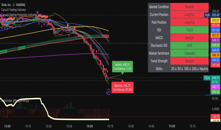
Example: TSLA Across Timeframes
Using live TSLA data (close ~346.46 USD, May 31, 2025), the indicator produces:
30-Minute: Bullish 341.93 (13.3%), Bearish 327.96 (86.7%) – Strong bearish sentiment due to intraday volatility.
1-Hour: Bullish 342.00 (33.9%), Bearish 327.50 (62.3%) – Bearish but less intense, reflecting hourly swings.
4-Hour: Bullish 345.52 (73.4%), Bearish 344.44 (19.0%) – Flat outlook, indicating consolidation.
Daily: Bullish 391.26 (68.8%), Bearish 302.22 (31.2%) – Bullish bias from recent uptrend, bearish tempered by longer lookback.
Weekly: Bullish 414.37 (35.0%), Bearish 279.08 (41.3%) – Wide range, reflecting annual volatility.
Monthly: Bullish 396.70 (54.9%), Bearish 296.93 (10.2%) – Long-term bullish optimism.
These results align with market dynamics: short-term intervals capture volatility, while longer intervals smooth trends, providing balanced outlooks.
Notes
Accuracy: Projections are estimates based on historical data and should be used with other analysis tools. Confidence levels indicate likelihood, not certainty.
Timeframe Sensitivity: Short-term intervals (e.g., 30-minute) show larger price swings and higher confidence due to volatility, while longer intervals (e.g., monthly) are more stable.
Customization: Adjust inputs to match your trading style (e.g., shorter lookback for day trading, longer for swing trading).
Performance: Tested on volatile stocks like TSLA, NVIDIA, and others, ensuring robust performance across markets.
Limitations: May produce conservative bearish projections in strong uptrends due to momentum weighting. Adjust lookback or projection_bars for sensitivity.
Feedback
If you encounter issues (e.g., label overlap, projection mismatches), please share your timeframe, settings, or a screenshot. Suggestions for enhancements (e.g., additional filters, visual tweaks) are welcome!
Disclaimer
The Canuck Trading Projection Indicator is provided for educational and informational purposes only. It is not financial advice. Trading involves significant risks, and past performance is not indicative of future results. Always perform your own due diligence and consult a qualified financial advisor before making trading decisions.
Cari dalam skrip untuk "20日线角度大于0的股票"

Supertrend with Volume Filter AlertSupertrend with Volume Filter Alert - Indicator Overview
What is the Supertrend Indicator?
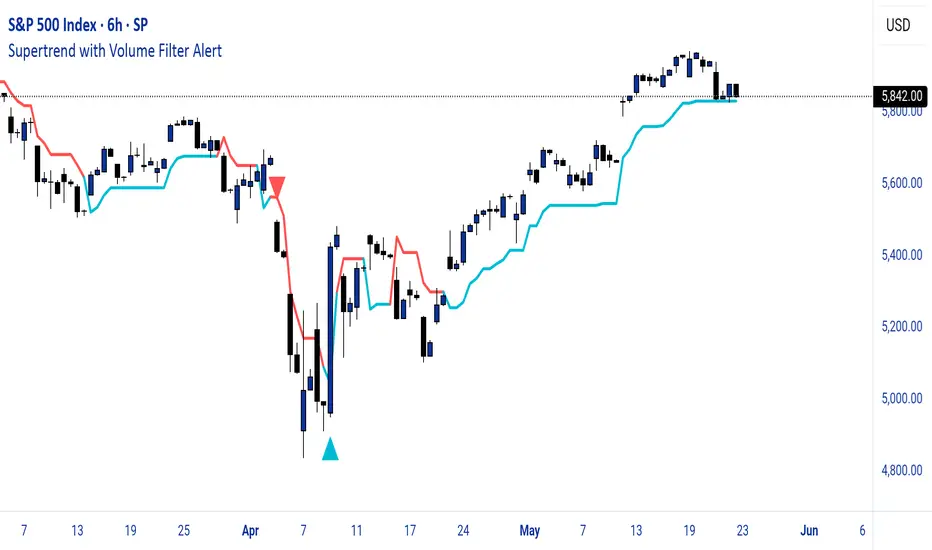
The Supertrend indicator is a popular trend-following tool used by traders to identify the direction of the market and potential entry/exit points. It is based on the Average True Range (ATR), which measures volatility, and plots a line on the chart that acts as a dynamic support or resistance level. When the price is above the Supertrend line, it signals an uptrend (bullish), and when the price is below, it indicates a downtrend (bearish). The indicator is particularly effective in trending markets but can generate false signals during choppy or sideways conditions.
How This Script Works
The "Supertrend with Volume Filter Alert" enhances the classic Supertrend indicator by adding a customizable volume filter to improve signal reliability.
Here's how it functions:
Supertrend Calculation:The Supertrend is calculated using the ATR over a user-defined period (default: 55) and a multiplier (default: 1.85). These parameters control the sensitivity of the indicator:A higher ATR period smooths out volatility, making the indicator less reactive to short-term price fluctuations.The multiplier determines the distance of the Supertrend line from the price, affecting how quickly it responds to trend changes.The script plots the Supertrend line in cyan for uptrends and red for downtrends, making it easy to visualize the market direction.
Volume Filter:A key feature of this script is the volume filter, which helps filter out false signals in choppy markets. The filter compares the current volume to the average volume over a lookback period (default: 20) and only triggers signals if the volume exceeds the average by a specified multiplier (default: 2.0).This ensures that trend changes are accompanied by significant market participation, increasing the likelihood of a genuine trend shift.
Signals and Alerts:
Buy signals (cyan triangle below the bar) are generated when the price crosses above the Supertrend line (indicating an uptrend) and the volume condition is met.Sell signals (red triangle above the bar) are generated when the price crosses below the Supertrend line (indicating a downtrend) and the volume condition is met.Alerts are set up for both buy and sell signals, notifying traders only when the volume filter confirms the trend change.
Customizable Settings for Multiple Markets
The default settings in this script (ATR Period: 55, ATR Multiplier: 1.85, Volume Lookback Period: 20, Volume Multiplier: 2.0) were carefully chosen to provide a balance of sensitivity and reliability across various markets, including stocks, indices (like the S&P 500), forex, and cryptocurrencies.
Here's why these settings work well:
ATR Period (55): A longer ATR period smooths out volatility, making the indicator less prone to whipsaws in volatile markets like crypto or forex, while still being responsive enough for trending markets like indices.
ATR Multiplier (1.85): This multiplier strikes a balance between capturing early trend changes and avoiding noise. A smaller multiplier would make the indicator too sensitive, while a larger one might miss early opportunities.
Volume Lookback Period (20): A 20-bar lookback for volume averaging provides a robust baseline for identifying significant volume spikes, adaptable to both short-term (e.g., daily charts) and longer-term (e.g., weekly charts) timeframes.
Volume Multiplier (2.0): Requiring volume to be at least 2x the average ensures that only high-conviction moves trigger signals, which is crucial for markets with varying liquidity levels.
These parameters are fully customizable, allowing traders to adjust the indicator to their specific market, timeframe, or trading style. For example, you might reduce the ATR period for faster-moving markets or increase the volume multiplier for more conservative signal filtering.
How the Volume Filter Reduces Bad Trades in Choppy Markets
One of the main drawbacks of the Supertrend indicator is its tendency to generate false signals during choppy or ranging markets, where price fluctuates without a clear trend. The volume filter in this script addresses this issue by ensuring that trend changes are backed by significant market activity:
In choppy markets, price movements often lack strong volume, leading to false breakouts or reversals. By requiring volume to be a multiple (default: 2x) of the average volume over the lookback period, the script filters out these low-volume, low-conviction moves.This reduces the likelihood of taking bad trades during sideways markets, as only trend changes with strong volume confirmation will trigger signals. For example, on a daily chart of the S&P 500, a buy signal will only fire if the price crosses above the Supertrend line and the volume on that day is at least twice the 20-day average, indicating genuine buying pressure.
Usage Tips
Markets and Timeframes: This indicator is versatile and can be used on various assets (stocks, indices, forex, crypto) and timeframes (1-minute, 1-hour, daily, etc.). Adjust the settings based on the market's volatility and your trading strategy.
Combine with Other Indicators: While the volume filter improves reliability, consider using additional indicators like RSI or MACD to confirm trends, especially in ranging markets.
Backtesting: Test the indicator on historical data for your chosen market to optimize the settings and ensure they align with your trading goals.
Alerts: Set up alerts for buy and sell signals to stay informed of high-probability trend changes without constantly monitoring the chart.
ConclusionThe "Supertrend with Volume Filter Alert" is a powerful tool for trend-following traders, combining the simplicity of the Supertrend indicator with a volume-based filter to enhance signal accuracy. Its customizable settings make it adaptable to multiple markets, while the volume filter helps reduce false signals in choppy conditions, allowing traders to focus on high-probability trades. Whether you're trading stocks, indices, forex, or crypto, this indicator can help you identify trends with greater confidence.
Levels & Flow📌 Overview
Levels & Flow is a visual trading tool that combines daily pivot levels with a dynamic EMA ribbon to help traders identify structure, momentum, and key decision zones in the market.
This script is designed for discretionary traders who rely on clean visual cues for intraday and swing trading strategies.
⚙️ Key Features
Daily Pivot, Support, and Resistance Lines
Automatically plots the daily pivot level based on the previous day’s OHLC data, along with calculated support and resistance levels.
Fibonacci Retracement Levels
Two dashed lines above and below the pivot represent the retracement of the pivot-resistance and pivot-support range, forming the boundaries of the “no-trade zone.”
No-Trade Zone (Shaded Box)
A gray shaded box between the two Fibonacci levels to visually mark a high-chop/low-conviction zone.
Trend-Based Candle Coloring (Current Day Only)
Candles are colored green if the close is above the pivot, red if below (only on the current trading day).
Bullish/Bearish Trend Label
A small table in the bottom-right corner displays “Bullish” or “Bearish” depending on whether price is above or below the pivot.
20-EMA Gradient Ribbon
A stack of 20 EMAs, each smoothed and color-coded from blue to green to reflect short- to long-term trend alignment.
Cumulative EMA with Adaptive Weighting
An intelligent moving average line that adjusts weight distribution among the 20 EMAs based on recent predictive accuracy using a learning rate and lookback period.
🧠 How It Works
📍 Levels
The script calculates daily pivot, resistance, and support levels using standard formulas:
Pivot = (High + Low + Close) / 3
Resistance = (2 × Pivot) – Low
Support = (2 × Pivot) – High
These levels update each day and extend 143 bars to the right.
📏 Fib Lines
Fib Up = Pivot + (Resistance – Pivot) × 0.382
Fib Down = Pivot – (Pivot – Support) × 0.382
These lines form the “no-trade zone” box.
📈 EMA Ribbon
20 EMAs starting from the user-defined Base Length, each incremented by 1
Each EMA is smoothed using the Smoothing Period
Color-coded from blue to green for intuitive visual flow
Filled between EMAs to visualize trend strength and alignment
🧠 Cumulative EMA Learning
Each EMA’s historical error is calculated over a Lookback Period
Lower-error EMAs receive higher weight; weights are normalized to sum to 1
The result is a cumulative EMA that adapts based on historical predictive power
🔧 User Inputs
Input
Base EMA Length: Sets the period for the shortest EMA (default: 20)
Smoothing Period: Smooths all EMAs and the cumulative EMA
Lookback for Learning: Number of bars to evaluate EMA prediction accuracy
Learning Rate: Adjusts how quickly weights shift in favor of more accurate EMAs
✅ How to Use It
Use the pivot level to define directional bias.
Watch for price breakouts above resistance or breakdowns below support to consider entry.
Avoid trading inside the shaded zone, where direction is less reliable.
Use the EMA ribbon gradient to confirm short/long alignment.
The cumulative EMA helps define trend with noise reduction.
🧪 Best For
Intraday traders who want to blend structure with flow
Swing traders needing clean daily levels with dynamic confirmation
Anyone looking to avoid choppy zones and improve visual clarity
⚠️ Disclaimer
This script is for educational and informational purposes only. It does not constitute financial advice or a trading recommendation. Always test scripts in simulation or on demo accounts before live use. Use at your own risk.
Canuck Trading IndicatorOverview
The Canuck Trading Indicator is a versatile, overlay-based technical analysis tool designed to assist traders in identifying potential trading opportunities across various timeframes and market conditions. By combining multiple technical indicators—such as RSI, Bollinger Bands, EMAs, VWAP, MACD, Stochastic RSI, ADX, HMA, and candlestick patterns—the indicator provides clear visual signals for bullish and bearish entries, breakouts, long-term trends, and options strategies like cash-secured puts, straddles/strangles, iron condors, and short squeezes. It also incorporates 20-day and 200-day SMAs to detect Golden/Death Crosses and price positioning relative to these moving averages. A dynamic table displays key metrics, and customizable alerts help traders stay informed of market conditions.
Key Features
Multi-Timeframe Adaptability: Automatically adjusts parameters (e.g., ATR multiplier, ADX period, HMA length) based on the chart's timeframe (minute, hourly, daily, weekly, monthly) for optimal performance.
Comprehensive Signal Generation: Identifies short-term entries, breakouts, long-term bullish trends, and options strategies using a combination of momentum, trend, volatility, and candlestick patterns.
Candlestick Pattern Detection: Recognizes bullish/bearish engulfing, hammer, shooting star, doji, and strong candles for precise entry/exit signals.
Moving Average Analysis: Plots 20-day and 200-day SMAs, detects Golden/Death Crosses, and evaluates price position relative to these averages.
Dynamic Table: Displays real-time metrics, including zone status (bullish, bearish, neutral), RSI, MACD, Stochastic RSI, short/long-term trends, candlestick patterns, ADX, ROC, VWAP slope, and MA positioning.
Customizable Alerts: Over 20 alert conditions for entries, exits, overbought/oversold warnings, and MA crosses, with actionable messages including ticker, price, and suggested strategies.
Visual Clarity: Uses distinct shapes, colors, and sizes to plot signals (e.g., green triangles for bullish entries, red triangles for bearish entries) and overlays key levels like EMA, VWAP, Bollinger Bands, support/resistance, and HMA.
Options Strategy Signals: Suggests opportunities for selling cash-secured puts, straddles/strangles, iron condors, and capitalizing on short squeezes.
How to Use
Add to Chart: Apply the indicator to any TradingView chart by selecting "Canuck Trading Indicator" from the Pine Script library.
Interpret Signals:
Bullish Signals: Green triangles (short-term entry), lime diamonds (breakout), blue circles (long-term entry).
Bearish Signals: Red triangles (short-term entry), maroon diamonds (breakout).
Options Strategies: Purple squares (cash-secured puts), yellow circles (straddles/strangles), orange crosses (iron condors), white arrows (short squeezes).
Exits: X-cross shapes in corresponding colors indicate exit signals.
Monitor: Gray circles suggest holding cash or monitoring for setups.
Review Table: Check the top-right table for real-time metrics, including zone status, RSI, MACD, trends, and MA positioning.
Set Alerts: Configure alerts for specific signals (e.g., "Short-Term Bullish Entry" or "Golden Cross") to receive notifications via TradingView.
Adjust Inputs: Customize input parameters (e.g., RSI period, EMA length, ATR period) to suit your trading style or market conditions.
Input Parameters
The indicator offers a wide range of customizable inputs to fine-tune its behavior:
RSI Period (default: 14): Length for RSI calculation.
RSI Bullish Low/High (default: 35/70): RSI thresholds for bullish signals.
RSI Bearish High (default: 65): RSI threshold for bearish signals.
EMA Period (default: 15): Main EMA length (15 for day trading, 50 for swing).
Short/Long EMA Length (default: 3/20): For momentum oscillator.
T3 Smoothing Length (default: 5): Smooths momentum signals.
Long-Term EMA/RSI Length (default: 20/15): For long-term trend analysis.
Support/Resistance Lookback (default: 5): Periods for support/resistance levels.
MACD Fast/Slow/Signal (default: 12/26/9): MACD parameters.
Bollinger Bands Period/StdDev (default: 15/2): BB settings.
Stochastic RSI Period/Smoothing (default: 14/3/3): Stochastic RSI settings.
Uptrend/Short-Term/Long-Term Lookback (default: 2/2/5): Candles for trend detection.
ATR Period (default: 14): For volatility and price targets.
VWAP Sensitivity (default: 0.1%): Threshold for VWAP-based signals.
Volume Oscillator Period (default: 14): For volume surge detection.
Pattern Detection Threshold (default: 0.3%): Sensitivity for candlestick patterns.
ROC Period (default: 3): Rate of change for momentum.
VWAP Slope Period (default: 5): For VWAP trend analysis.
TradingView Publishing Compliance
Originality: The Canuck Trading Indicator is an original script, combining multiple technical indicators and custom logic to provide unique trading signals. It does not replicate existing public scripts.
No Guaranteed Profits: This indicator is a tool for technical analysis and does not guarantee profits. Trading involves risks, and users should conduct their own research and risk management.
Clear Instructions: The description and usage guide are detailed and accessible, ensuring users understand how to apply the indicator effectively.
No External Dependencies: The script uses only built-in Pine Script functions (e.g., ta.rsi, ta.ema, ta.vwap) and requires no external libraries or data sources.
Performance: The script is optimized for performance, using efficient calculations and adaptive parameters to minimize lag on various timeframes.
Visual Clarity: Signals are plotted with distinct shapes and colors, and the table provides a concise summary of market conditions, enhancing usability.
Limitations and Risks
Market Conditions: The indicator may generate false signals in choppy or low-liquidity markets. Always confirm signals with additional analysis.
Timeframe Sensitivity: Performance varies by timeframe; test settings on your preferred chart (e.g., 5-minute for day trading, daily for swing trading).
Risk Management: Use stop-losses and position sizing to manage risk, as suggested in alert messages (e.g., "Stop -20%").
Options Trading: Options strategies (e.g., straddles, iron condors) carry unique risks; consult a financial advisor before trading.
Feedback and Support
For questions, suggestions, or bug reports, please leave a comment on the TradingView script page or contact the author via TradingView. Your feedback helps improve the indicator for the community.
Disclaimer
The Canuck Trading Indicator is provided for educational and informational purposes only. It is not financial advice. Trading involves significant risks, and past performance is not indicative of future results. Always perform your own due diligence and consult a qualified financial advisor before making trading decisions.
Enhanced Volume Trend Indicator with BB SqueezeEnhanced Volume Trend Indicator with BB Squeeze: Comprehensive Explanation
The visualization system allows traders to quickly scan multiple securities to identify high-probability setups without detailed analysis of each chart. The progression from squeeze to breakout, supported by volume trend confirmation, offers a systematic approach to identifying trading opportunities.
The script combines multiple technical analysis approaches into a comprehensive dashboard that helps traders make informed decisions by identifying high-probability setups while filtering out noise through its sophisticated confirmation requirements. It combines multiple technical analysis approaches into an integrated visual system that helps traders identify potential trading opportunities while filtering out false signals.
Core Features
1. Volume Analysis Dashboard
The indicator displays various volume-related metrics in customizable tables:
AVOL (After Hours + Pre-Market Volume): Shows extended hours volume as a percentage of the 21-day average volume with color coding for buying/selling pressure. Green indicates buying pressure and red indicates selling pressure.
Volume Metrics: Includes regular volume (VOL), dollar volume ($VOL), relative volume compared to 21-day average (RVOL), and relative volume compared to 90-day average (RVOL90D).
Pre-Market Data: Optional display of pre-market volume (PVOL), pre-market dollar volume (P$VOL), pre-market relative volume (PRVOL), and pre-market price change percentage (PCHG%).
2. Enhanced Volume Trend (VTR) Analysis
The Volume Trend indicator uses adaptive analysis to evaluate buying and selling pressure, combining multiple factors:
MACD (Moving Average Convergence Divergence) components
Volume-to-SMA (Simple Moving Average) ratio
Price direction and market conditions
Volume change rates and momentum
EMA (Exponential Moving Average) alignment and crossovers
Volatility filtering
VTR Visual Indicators
The VTR score ranges from 0-100, with values above 50 indicating bullish conditions and below 50 indicating bearish conditions. This is visually represented by colored circles:
"●" (Filled Circle):
Green: Strong bullish trend (VTR ≥ 80)
Red: Strong bearish trend (VTR ≤ 20)
"◯" (Hollow Circle):
Green: Moderate bullish trend (VTR 65-79)
Red: Moderate bearish trend (VTR 21-35)
"·" (Small Dot):
Green: Weak bullish trend (VTR 55-64)
Red: Weak bearish trend (VTR 36-45)
"○" (Medium Hollow Circle): Neutral conditions (VTR 46-54), shown in gray
In "Both" display mode, the VTR shows both the numerical score (0-100) alongside the appropriate circle symbol.
Enhanced VTR Settings
The Enhanced Volume Trend component offers several advanced customization options:
Adaptive Volume Analysis (volTrendAdaptive):
When enabled, dynamically adjusts volume thresholds based on recent market volatility
Higher volatility periods require proportionally higher volume to generate significant signals
Helps prevent false signals during highly volatile markets
Keep enabled for most trading conditions, especially in volatile markets
Speed of Change Weight (volTrendSpeedWeight, range 0-1):
Controls emphasis on volume acceleration/deceleration rather than absolute levels
Higher values (0.7-1.0): More responsive to new volume trends, better for momentum trading
Lower values (0.2-0.5): Less responsive, better for trend following
Helps identify early volume trends before they fully develop
Momentum Period (volTrendMomentumPeriod, range 2-10):
Defines lookback period for volume change rate calculations
Lower values (2-3): More responsive to recent changes, better for short timeframes
Higher values (7-10): Smoother, better for daily/weekly charts
Directly affects how quickly the indicator responds to new volume patterns
Volatility Filter (volTrendVolatilityFilter):
Adjusts significance of volume by factoring in current price volatility
High volume during high volatility receives less weight
High volume during low volatility receives more weight
Helps distinguish between genuine volume-driven moves and volatility-driven moves
EMA Alignment Weight (volTrendEmaWeight, range 0-1):
Controls importance of EMA alignments in final VTR calculation
Analyzes multiple EMA relationships (5, 10, 21 period)
Higher values (0.7-1.0): Greater emphasis on trend structure
Lower values (0.2-0.5): More focus on pure volume patterns
Display Mode (volTrendDisplayMode):
"Value": Shows only numerical score (0-100)
"Strength": Shows only symbolic representation
"Both": Shows numerical score and symbol together
3. Bollinger Band Squeeze Detection (SQZ)
The BB Squeeze indicator identifies periods of low volatility when Bollinger Bands contract inside Keltner Channels, often preceding significant price movements.
SQZ Visual Indicators
"●" (Filled Circle): Strong squeeze - high probability setup for an impending breakout
Green: Strong squeeze with bullish bias (likely upward breakout)
Red: Strong squeeze with bearish bias (likely downward breakout)
Orange: Strong squeeze with unclear direction
"◯" (Hollow Circle): Moderate squeeze - medium probability setup
Green: With bullish EMA alignment
Red: With bearish EMA alignment
Orange: Without clear directional bias
"-" (Dash): Gray dash indicates no squeeze condition (normal volatility)
The script identifies squeeze conditions through multiple methods:
Bollinger Bands contracting inside Keltner Channels
BB width falling to bottom 20% of recent range (BB width percentile)
Very narrow Keltner Channel (less than 5% of basis price)
Tracking squeeze duration in consecutive bars
Different squeeze strengths are detected:
Strong Squeeze: BB inside KC with tight BB width and narrow KC
Moderate Squeeze: BB inside KC with either tight BB width or narrow KC
No Squeeze: Normal market conditions
4. Breakout Detection System
The script includes two breakout indicators working in sequence:
4.1 Pre-Breakout (PBK) Indicator
Detects potential upcoming breakouts by analyzing multiple factors:
Squeeze conditions lasting 2-3 bars or more
Significant price ranges
Strong volume confirmation
EMA/MACD crossovers
Consistent price direction
PBK Visual Indicators
"●" (Filled Circle): Detected pre-breakout condition
Green: Likely upward breakout (bullish)
Red: Likely downward breakout (bearish)
Orange: Direction not yet clear, but breakout likely
"-" (Dash): Gray dash indicates no pre-breakout condition
The PBK uses sophisticated conditions to reduce false signals including minimum squeeze length, significant price movement, and technical confirmations.
4.2 Breakout (BK) Indicator
Confirms actual breakouts in progress by identifying:
End of squeeze or strong expansion of Bollinger Bands
Volume expansion
Price moving outside Bollinger Bands
EMA crossovers with volume confirmation
MACD crossovers with significant price range
BK Visual Indicators
"●" (Filled Circle): Confirmed breakout in progress
Green: Upward breakout (bullish)
Red: Downward breakout (bearish)
Orange: Unusual breakout pattern without clear direction
"◆" (Diamond): Special breakout conditions (meets some but not all criteria)
"-" (Dash): Gray dash indicates no breakout detected
The BK indicator uses advanced filters for confirmation:
Requires consecutive breakout signals to reduce false positives
Strong volume confirmation requirements (40% above average)
Significant price movement thresholds
Consistency checks between price action and indicators
5. Market Metrics and Analysis
Price Change Percentage (CHG%)
Displays the current percentage change relative to the previous day's close, color-coded green for positive changes and red for negative changes.
Average Daily Range (ADR%)
Calculates the average daily percentage range over a specified period (default 20 days), helping traders gauge volatility and set appropriate price targets.
Average True Range (ATR)
Shows the Average True Range value, a volatility indicator developed by J. Welles Wilder that measures market volatility by decomposing the entire range of an asset price for that period.
Relative Strength Index (RSI)
Displays the standard 14-period RSI, a momentum oscillator that measures the speed and change of price movements on a scale from 0 to 100.
6. External Market Indicators
QQQ Change
Shows the percentage change in the Invesco QQQ Trust (tracking the Nasdaq-100 Index), useful for understanding broader tech market trends.
UVIX Change
Displays the percentage change in UVIX, a volatility index, providing insight into market fear and potential hedging activity.
BTC-USD
Shows the current Bitcoin price from Coinbase, useful for traders monitoring crypto correlation with equities.
Market Breadth (BRD)
Calculates the percentage difference between ATHI.US and ATLO.US (high vs. low securities), indicating overall market direction and strength.
7. Session Analysis and Volume Direction
Session Detection
The script accurately identifies different market sessions:
Pre-market: 4:00 AM to 9:30 AM
Regular market: 9:30 AM to 4:00 PM
After-hours: 4:00 PM to 8:00 PM
Closed: Outside trading hours
This detection works on any timeframe through careful calculation of current time in seconds.
Buy/Sell Volume Direction
The script analyzes buying and selling pressure by:
Counting up volume when close > open
Counting down volume when close < open
Tracking accumulated volume within the day
Calculating intraday pressure (up volume minus down volume)
Enhanced AVOL Calculation
The improved AVOL calculation works in all timeframes by:
Estimating typical pre-market and after-hours volume percentages
Combining yesterday's after-hours with today's pre-market volume
Calculating this as a percentage of the 21-day average volume
Determining buying/selling pressure by analyzing after-hours and pre-market price changes
Color-coding results: green for buying pressure, red for selling pressure
This calculation is particularly valuable because it works consistently across any timeframe.
Customization Options
Display Settings
The dashboard has two customizable tables: Volume Table and Metrics Table, with positions selectable as bottom_left or bottom_right.
All metrics can be individually toggled on/off:
Pre-market data (PVOL, P$VOL, PRVOL, PCHG%)
Volume data (AVOL, RVOL Day, RVOL 90D, Volume, SEED_YASHALGO_NSE_BREADTH:VOLUME )
Price metrics (ADR%, ATR, RSI, Price Change%)
Market indicators (QQQ, UVIX, Breadth, BTC-USD)
Analysis indicators (Volume Trend, BB Squeeze, Pre-Breakout, Breakout)
These toggle options allow traders to customize the dashboard to show only the metrics they find most valuable for their trading style.
Table and Text Customization
The dashboard's appearance can be customized:
Table background color via tableBgColor
Text color (White or Black) via textColorOption
The indicator uses smart formatting for volume and price values, automatically adding appropriate suffixes (K, M, B) for readability.
MACD Configuration for VTR
The Volume Trend calculation incorporates MACD with customizable parameters:
Fast Length: Controls the period for the fast EMA (default 3)
Slow Length: Controls the period for the slow EMA (default 9)
Signal Length: Controls the period for the signal line EMA (default 5)
MACD Weight: Controls how much influence MACD has on the volume trend score (default 0.3)
These settings allow traders to fine-tune how momentum is factored into the volume trend analysis.
Bollinger Bands and Keltner Channel Settings
The Bollinger Bands and Keltner Channels used for squeeze detection have preset (hidden) parameters:
BB Length: 20 periods
BB Multiplier: 2.0 standard deviations
Keltner Length: 20 periods
Keltner Multiplier: 1.5 ATR
These settings follow standard practice for squeeze detection while maintaining simplicity in the user interface.
Practical Trading Applications
Complete Trading Strategies
1. Squeeze Breakout Strategy
This strategy combines multiple components of the indicator:
Wait for a strong squeeze (SQZ showing ●)
Look for pre-breakout confirmation (PBK showing ● in green or red)
Enter when breakout is confirmed (BK showing ● in same direction)
Use VTR to confirm volume supports the move (VTR ≥ 65 for bullish or ≤ 35 for bearish)
Set profit targets based on ADR (Average Daily Range)
Exit when VTR begins to weaken or changes direction
2. Volume Divergence Strategy
This strategy focuses on the volume trend relative to price:
Identify when price makes a new high but VTR fails to confirm (divergence)
Look for VTR to show weakening trend (● changing to ◯ or ·)
Prepare for potential reversal when SQZ begins to form
Enter counter-trend position when PBK confirms reversal direction
Use external indicators (QQQ, BTC, Breadth) to confirm broader market support
3. Pre-Market Edge Strategy
This strategy leverages pre-market data:
Monitor AVOL for unusual pre-market activity (significantly above 100%)
Check pre-market price change direction (PCHG%)
Enter position at market open if VTR confirms direction
Use SQZ to determine if volatility is likely to expand
Exit based on RVOL declining or price reaching +/- ADR for the day
Market Context Integration
The indicator provides valuable context for trading decisions:
QQQ change shows tech market direction
BTC price shows crypto market correlation
UVIX change indicates volatility expectations
Breadth measurement shows market internals
This context helps traders avoid fighting the broader market and align trades with overall market direction.
Timeframe Optimization
The indicator is designed to work across different timeframes:
For day trading: Focus on AVOL, VTR, PBK/BK, and use shorter momentum periods
For swing trading: Focus on SQZ duration, VTR strength, and broader market indicators
For position trading: Focus on larger VTR trends and use EMA alignment weight
Advanced Analytical Components
Enhanced Volume Trend Score Calculation
The VTR score calculation is sophisticated, with the base score starting at 50 and adjusting for:
Price direction (up/down)
Volume relative to average (high/normal/low)
Volume acceleration/deceleration
Market conditions (bull/bear)
Additional factors are then applied, including:
MACD influence weighted by strength and direction
Volume change rate influence (speed)
Price/volume divergence effects
EMA alignment scores
Volatility adjustments
Breakout strength factors
Price action confirmations
The final score is clamped between 0-100, with values above 50 indicating bullish conditions and below 50 indicating bearish conditions.
Anti-False Signal Filters
The indicator employs multiple techniques to reduce false signals:
Requiring significant price range (minimum percentage movement)
Demanding strong volume confirmation (significantly above average)
Checking for consistent direction across multiple indicators
Requiring prior bar consistency (consecutive bars moving in same direction)
Counting consecutive signals to filter out noise
These filters help eliminate noise and focus on high-probability setups.
MACD Enhancement and Integration
The indicator enhances standard MACD analysis:
Calculating MACD relative strength compared to recent history
Normalizing MACD slope relative to volatility
Detecting MACD acceleration for stronger signals
Integrating MACD crossovers with other confirmation factors
EMA Analysis System
The indicator uses a comprehensive EMA analysis system:
Calculating multiple EMAs (5, 10, 21 periods)
Detecting golden cross (10 EMA crosses above 21 EMA)
Detecting death cross (10 EMA crosses below 21 EMA)
Assessing price position relative to EMAs
Measuring EMA separation percentage
Recent Enhancements and Evolution
Version 5.2 includes several improvements:
Enhanced AVOL to show buying/selling direction through color coding
Improved VTR with adaptive analysis based on market conditions
AVOL display now works in all timeframes through sophisticated estimation
Removed animal symbols and streamlined code with bright colors for better visibility
Improved anti-false signal filters throughout the system
Optimizing Indicator Settings
For Different Market Types
Range-Bound Markets:
Lower EMA Alignment Weight (0.2-0.4)
Higher Speed of Change Weight (0.8-1.0)
Focus on SQZ and PBK signals for breakout potential
Trending Markets:
Higher EMA Alignment Weight (0.7-1.0)
Moderate Speed of Change Weight (0.4-0.6)
Focus on VTR strength and BK confirmations
Volatile Markets:
Enable Volatility Filter
Enable Adaptive Volume Analysis
Lower Momentum Period (2-3)
Focus on strong volume confirmation (VTR ≥ 80 or ≤ 20)
For Different Asset Classes
Equities:
Standard settings work well
Pay attention to AVOL for gap potential
Monitor QQQ correlation
Futures:
Consider higher Volume/RVOL weight
Reduce MACD weight slightly
Pay close attention to SQZ duration
Crypto:
Higher volatility thresholds may be needed
Monitor BTC price for correlation
Focus on stronger confirmation signals
Integrated Visual System for Trading Decisions
The colored circle indicators create an intuitive visual system for quick market assessment:
Progression Sequence: SQZ (Squeeze) → PBK (Pre-Breakout) → BK (Breakout)
This sequence often occurs in order, with the squeeze leading to pre-breakout conditions, followed by an actual breakout.
VTR (Volume Trend): Provides context about the volume supporting these movements.
Color Coding: Green for bullish conditions, red for bearish conditions, and orange/gray for neutral or undefined conditions.
ADR Nivele Horizontale dhe EMAThe user provided a Pine Script code for an indicator called "ADR Nivele Horizontale dhe EMA". The task is to explain how this code works. Hmm, first, I need to understand what this indicator does. The title mentions ADR levels and EMA, so it's probably combining horizontal lines based on Average Daily Range and some Exponential Moving Averages.
Looking at the code, the first part is the indicator declaration with version 6. The settings include an ADR period, levels above and below the mid, and line style. Then there's a section for calculations. They request daily high and low to compute the daily range. The ADR is the SMA of the daily range over the specified period. The mid is the average of daily high and low. The adr_val is half of ADR, maybe to create symmetrical levels around the mid.
Next, they create arrays for lines and labels above and below the mid. The loops go from 1 to levels_above/below, calculate each level, draw lines and labels. The mid line is also drawn with a different color. Then, there are several EMAs plotted: 13, 50, 200, 400, 600, 800, each with different colorsWait, but in Pine Script, when you use arrays to store lines and labels, you have to manage them properly to avoid repainting or memory issues. The code uses array.concat to add new lines and labels each bar. However, since this code is running on each bar, the for loops might be creating multiple lines each time, leading to too many objects. Oh right, but they use var to initialize the arrays, so they are only initialized once. Wait, no. The var keyword initializes the variable once, but in each iteration, they are concatenating new lines. Wait, no: the for loops are inside the main script, which runs on each bar. So every time a new bar is processed, the loops will run again, adding new lines and labels. That's a problem because each bar would create new lines, leading to an ever-increasing number of lines, which could hit the maximum limit (max_lines_count is set to 20, but maybe they have more bars). Oh, the indicator has max_lines_count=20, but the code might be creating multiple lines per bar. So maybe the code isn't handling the line management correctly. For example, if levels_above is 2, then each bar would create 2 new lines above and 2 below, plus the mid line. Over 20 bars, that's way over 20 lines. So this could cause the indicator to stop drawing after 20 lines. The user might not have realized that the lines are being recreated every bar, leading to a buildup. But perhaps the original code intended to have the lines update each bar, extending to the current bar. Let's see: in line.new, they use bar_index as the starting x1 and bar_index as x2. So each line is drawn from the previous bar's index to the current one. But since this is done on every bar, each line is only one bar long. Wait, no. Because on each new bar, the code creates a new line from the previous bar's index (bar_index , which is now the bar before the current one) to the current bar_index. So each line is just a segment from the previous bar to the current bar. But when the next bar comes, a new line is created again. So the result is that each level line is a series of one-bar-length segments, which might not be intended. The user probably wants continuous lines that extend from the left to the right, not just per bar. So this approach is incorrect. The correct way would be to have a line that starts at the first bar of the calculation and extends to the right, updating each bar. But the current code creates a new line each bar, leading to multiple short lines instead of one continuous line. That's a mistake.
So the main issue here is that the code is generating a new line segment for each bar, which is not efficient and would quickly hit the line limit. To fix this, instead of creating a new line every bar, they should create the line once and then update its position each bar. But in Pine Script, you can't directly update a line after it's created; instead, you need to track the line ID and use line.set_xy() to extend it. However, the current code uses array.concat to add new lines each bar, which isn't the right approach.
Therefore, the code as written will create multiple short lines instead of continuous horizontal lines. The correct approach for horizontal levels that extend to the right is to create the line once, starting at a certain bar and extending indefinitely, or to update the line's end point each new bar. But in Pine Script, you can't extend lines infinitely; you have to manage them each bar. Alternatively, using the 'line.extend' style might help, but I think the original code's logic is flawed here.
Additionally, the EMA part is straightforward: plotting multiple EMAs with different periods. That part should work as expected.
So the explanation should mention that the ADR levels are calculated based on the daily high and low, then the code attempts to draw horizontal lines above and below the mid-point. However, the way the lines are drawn may lead to multiple short segments instead of continuous lines, potentially causing performance issues or hitting the maximum line count. The EMAs are plotted correctly with various periods..

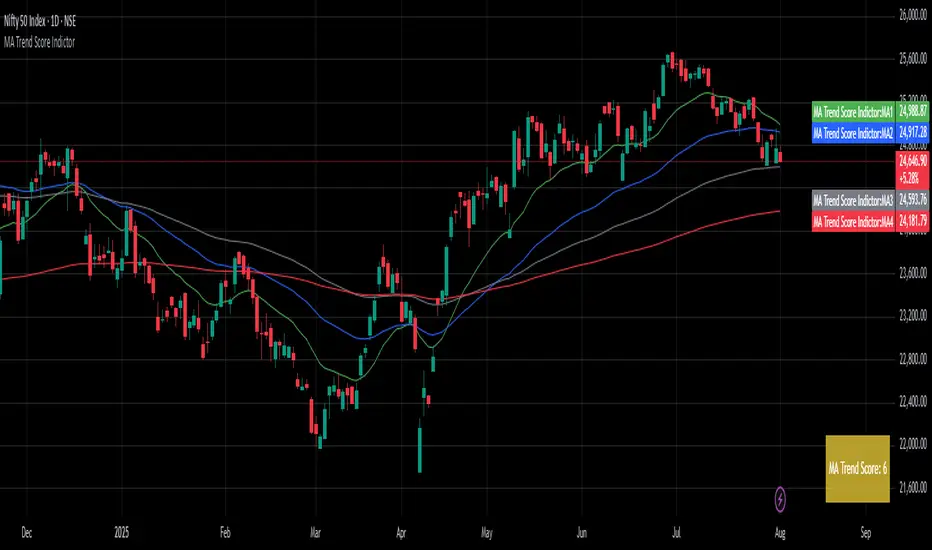
MA Trend ScoreA Trend Score Indicator inspired by an interview by Navy Ramavat, where I liked the idea presented and decided to publish a script for it.
Disclaimer: I am not associated with Navy Ramavat in any manner.
The goal is to objectify the trend of an instrument and calculate a score which represents the trend strength and direction.
The score is calculated as follows:
If price is > EMA 20 add 1 to the score
If price is > EMA 50 add 1 to the score
If price is > EMA 100 add 1 to the score
If EMA 20 is > EMA 50 add 1 to the score
If EMA 20 is > EMA 100 add 1 to the score
If EMA 50 is > EMA 100 add 1 to the score
If EMA 20 is < EMA 50 deduct 1 from the score
If EMA 20 is < EMA 100 deduct 1 from the score
If EMA 50 is < EMA 100 deduct 1 from the score
The highest score can be 6, and lowest score can be -6
The trend score can be used as per your discretion on the long and short side.
An example of using the trend score on the long side for position sizing is:
100% position size if Score greater than 4
75% position size if Score between 2-4
50% position size if Score between 0-2
25% position size if Score between 0 and -2
0% position size if Score is less than -2
Pivot S/R with Volatility Filter## *📌 Indicator Purpose*
This indicator identifies *key support/resistance levels* using pivot points while also:
✅ Detecting *high-volume liquidity traps* (stop hunts)
✅ Filtering insignificant pivots via *ATR (Average True Range) volatility*
✅ Tracking *test counts and breakouts* to measure level strength
---
## *⚙ SETTINGS – Detailed Breakdown*
### *1️⃣ ◆ General Settings*
#### *🔹 Pivot Length*
- *Purpose:* Determines how many bars to analyze when identifying pivots.
- *Usage:*
- *Low values (5-20):* More pivots, better for scalping.
- *High values (50-200):* Fewer but stronger levels for swing trading.
- *Example:*
- Pivot Length = 50 → Only the most significant highs/lows over 50 bars are marked.
#### *🔹 Test Threshold (Max Test Count)*
- *Purpose:* Sets how many times a level can be tested before being invalidated.
- *Example:*
- Test Threshold = 3 → After 3 tests, the level is ignored (likely to break).
#### *🔹 Zone Range*
- *Purpose:* Creates a price buffer around pivots (±0.001 by default).
- *Why?* Markets often respect "zones" rather than exact prices.
---
### *2️⃣ ◆ Volatility Filter (ATR)*
#### *🔹 ATR Period*
- *Purpose:* Smoothing period for Average True Range calculation.
- *Default:* 14 (standard for volatility measurement).
#### *🔹 ATR Multiplier (Min Move)*
- *Purpose:* Requires pivots to show *meaningful price movement*.
- *Formula:* Min Move = ATR × Multiplier
- *Example:*
- ATR = 10 pips, Multiplier = 1.5 → Only pivots with *15+ pip swings* are valid.
#### *🔹 Show ATR Filter Info*
- Displays current ATR and minimum move requirements on the chart.
---
### *3️⃣ ◆ Volume Analysis*
#### *🔹 Volume Change Threshold (%)*
- *Purpose:* Filters for *unusual volume spikes* (institutional activity).
- *Example:*
- Threshold = 1.2 → Requires *120% of average volume* to confirm signals.
#### *🔹 Volume MA Period*
- *Purpose:* Lookback period for "normal" volume calculation.
---
### *4️⃣ ◆ Wick Analysis*
#### *🔹 Wick Length Threshold (Ratio)*
- *Purpose:* Ensures rejection candles have *long wicks* (strong reversals).
- *Formula:* Wick Ratio = (Upper Wick + Lower Wick) / Candle Range
- *Example:*
- Threshold = 0.6 → 60% of the candle must be wicks.
#### *🔹 Min Wick Size (ATR %)*
- *Purpose:* Filters out small wicks in volatile markets.
- *Example:*
- ATR = 20 pips, MinWickSize = 1% → Wicks under *0.2 pips* are ignored.
---
### *5️⃣ ◆ Display Settings*
- *Show Zones:* Toggles support/resistance shaded areas.
- *Show Traps:* Highlights liquidity traps (▲/▼ symbols).
- *Show Tests:* Displays how many times levels were tested.
- *Zone Transparency:* Adjusts opacity of zones.
---
## *🎯 Practical Use Cases*
### *1️⃣ Liquidity Trap Detection*
- *Scenario:* Price spikes *above resistance* then reverses sharply.
- *Requirements:*
- Long wick (Wick Ratio > 0.6)
- High volume (Volume > Threshold)
- *Outcome:* *Short Trap* signal (▼) appears.
### *2️⃣ Strong Support Level*
- *Scenario:* Price bounces *3 times* from the same level.
- *Indicator Action:*
- Labels the level with test count (3/5 = 3 tests out of max 5).
- Turns *red* if broken (Break Count > 0).
Deep Dive: How This Indicator Works*
This indicator combines *four professional trading concepts* into one powerful tool:
1. *Classic Pivot Point Theory*
- Identifies swing highs/lows where price previously reversed
- Unlike basic pivot indicators, ours uses *confirmed pivots only* (filtered by ATR)
2. *Volume-Weighted Validation*
- Requires unusual trading volume to confirm levels
- Filters out "phantom" levels with low participation
3. *ATR Volatility Filtering*
- Eliminates insignificant price swings in choppy markets
- Ensures only meaningful levels are plotted
4. *Liquidity Trap Detection*
- Spots institutional stop hunts where markets fake out traders
- Uses wick analysis + volume spikes for high-probability signals
---
## *📊 Parameter Encyclopedia (Expanded)*
### *1️⃣ Pivot Engine Settings*
#### *Pivot Length (50)*
- *What It Does:*
Determines how many bars to analyze when searching for swing highs/lows.
- *Professional Adjustment Guide:*
| Trading Style | Recommended Value | Why? |
|--------------|------------------|------|
| Scalping | 10-20 | Captures short-term levels |
| Day Trading | 30-50 | Balanced approach |
| Swing Trading| 50-200 | Focuses on major levels |
- *Real Market Example:*
On NASDAQ 5-minute chart:
- Length=20: Identifies levels holding for ~2 hours
- Length=50: Finds levels respected for entire trading day
#### *Test Threshold (5)*
- *Advanced Insight:*
Institutions often test levels 3-5 times before breaking them. This setting mimics the "probe and push" strategy used by smart money.
- *Psychology Behind It:*
Retail traders typically give up after 2-3 tests, while institutions keep testing until stops are run.
---
### *2️⃣ Volatility Filter System*
#### *ATR Multiplier (1.0)*
- *Professional Formula:*
Minimum Valid Swing = ATR(14) × Multiplier
- *Market-Specific Recommendations:*
| Market Type | Optimal Multiplier |
|------------------|--------------------|
| Forex Majors | 0.8-1.2 |
| Crypto (BTC/ETH) | 1.5-2.5 |
| SP500 Stocks | 1.0-1.5 |
- *Why It Matters:*
In EUR/USD (ATR=10 pips):
- Multiplier=1.0 → Requires 10 pip swings
- Multiplier=1.5 → Requires 15 pip swings (fewer but higher quality levels)
---
### *3️⃣ Volume Confirmation System*
#### *Volume Threshold (1.2)*
- *Institutional Benchmark:*
- 1.2x = Moderate institutional interest
- 1.5x+ = Strong smart money activity
- *Volume Spike Case Study:*
*Before Apple Earnings:*
- Normal volume: 2M shares
- Spike threshold (1.2): 2.4M shares
- Actual volume: 3.1M shares → STRONG confirmation
---
### *4️⃣ Liquidity Trap Detection*
#### *Wick Analysis System*
- *Two-Filter Verification:*
1. *Wick Ratio (0.6):*
- Ensures majority of candle shows rejection
- Formula: (UpperWick + LowerWick) / Total Range > 0.6
2. *Min Wick Size (1% ATR):*
- Prevents false signals in flat markets
- Example: ATR=20 pips → Min wick=0.2 pips
- *Trap Identification Flowchart:*
Price Enters Zone →
Spikes Beyond Level →
Shows Long Wick →
Volume > Threshold →
TRAP CONFIRMED
---
## *💡 Master-Level Usage Techniques*
### *Institutional Order Flow Analysis*
1. *Step 1:* Identify pivot levels with ≥3 tests
2. *Step 2:* Watch for volume contraction near levels
3. *Step 3:* Enter when trap signal appears with:
- Wick > 2×ATR
- Volume > 1.5× average
### *Multi-Timeframe Confirmation*
1. *Higher TF:* Find weekly/monthly pivots
2. *Lower TF:* Use this indicator for precise entries
3. *Example:*
- Weekly pivot at $180
- 4H shows liquidity trap → High-probability reversal
---
## *⚠ Critical Mistakes to Avoid*
1. *Using Default Settings Everywhere*
- Crude oil needs higher ATR multiplier than bonds
2. *Ignoring Trap Context*
- Traps work best at:
- All-time highs/lows
- Major psychological numbers (00/50 levels)
3. *Overlooking Cumulative Volume*
- Check if volume is building over multiple tests

ETH/USDT EMA Crossover Strategy - OptimizedStrategy Name: EMA Crossover Strategy for ETH/USDT
Description:
This trading strategy is designed for the ETH/USDT pair and is based on exponential moving average (EMA) crossovers combined with momentum and volatility indicators. The strategy uses multiple filters to identify high-probability signals in both bullish and bearish trends, making it suitable for traders looking to trade in trending markets.
Strategy Components
EMAs (Exponential Moving Averages):
EMA 200: Used to identify the primary trend. If the price is above the EMA 200, it is considered a bullish trend; if below, a bearish trend.
EMA 50: Acts as an additional filter to confirm the trend.
EMA 20 and EMA 50 Short: These short-term EMAs generate entry signals through crossovers. A bullish crossover (EMA 20 crosses above EMA 50 Short) is a buy signal, while a bearish crossover (EMA 20 crosses below EMA 50 Short) is a sell signal.
RSI (Relative Strength Index):
The RSI is used to avoid overbought or oversold conditions. Long trades are only taken when the RSI is above 30, and short trades when the RSI is below 70.
ATR (Average True Range):
The ATR is used as a volatility filter. Trades are only taken when there is sufficient volatility, helping to avoid false signals in quiet markets.
Volume:
A volume filter is used to confirm sufficient market participation in the price movement. Trades are only taken when volume is above average.
Strategy Logic
Long Trades:
The price must be above the EMA 200 (bullish trend).
The EMA 20 must cross above the EMA 50 Short.
The RSI must be above 30.
The ATR must indicate sufficient volatility.
Volume must be above average.
Short Trades:
The price must be below the EMA 200 (bearish trend).
The EMA 20 must cross below the EMA 50 Short.
The RSI must be below 70.
The ATR must indicate sufficient volatility.
Volume must be above average.
How to Use the Strategy
Setup:
Add the script to your ETH/USDT chart on TradingView.
Adjust the parameters according to your preferences (e.g., EMA periods, RSI, ATR, etc.).
Signals:
Buy and sell signals will be displayed directly on the chart.
Long trades are indicated with an upward arrow, and short trades with a downward arrow.
Risk Management:
Use stop-loss and take-profit orders in all trades.
Consider a risk-reward ratio of at least 1:2.
Backtesting:
Test the strategy on historical data to evaluate its performance before using it live.
Advantages of the Strategy
Trend-focused: The strategy is designed to trade in trending markets, increasing the probability of success.
Multiple filters: The use of RSI, ATR, and volume reduces false signals.
Adaptability: It can be adjusted for different timeframes, although it is recommended to test it on 5-minute and 15-minute charts for ETH/USDT.
Warnings
Sideways markets: The strategy may generate false signals in markets without a clear trend. It is recommended to avoid trading in such conditions.
Optimization: Make sure to optimize the parameters according to the market and timeframe you are using.
Risk management: Never trade without stop-loss and take-profit orders.
Author
Jose J. Sanchez Cuevas
Version
v1.0

Enhanced KLSE Banker Flow Oscillator# Enhanced KLSE Banker Flow Oscillator
## Description
The Enhanced KLSE Banker Flow Oscillator is a sophisticated technical analysis tool designed specifically for the Malaysian stock market (KLSE). This indicator analyzes price and volume relationships to identify potential smart money movements, providing early signals for market reversals and continuation patterns.
The oscillator measures the buying and selling pressure in the market with a focus on detecting institutional activity. By combining money flow calculations with volume filters and price action analysis, it helps traders identify high-probability trading opportunities with reduced noise.
## Key Features
- Dual-Timeframe Analysis: Combines long-term money flow trends with short-term momentum shifts for more accurate signals
- Adaptive Volume Filtering: Automatically adjusts volume thresholds based on recent market conditions
- Advanced Divergence Detection: Identifies potential trend reversals through price-flow divergences
- Early Signal Detection: Provides anticipatory signals before major price movements occur
- Multiple Signal Types: Offers both early alerts and strong confirmation signals with clear visual markers
- Volatility Adjustment: Adapts sensitivity based on current market volatility for more reliable signals
- Comprehensive Visual Feedback: Color-coded oscillator, signal markers, and optional text labels
- Customizable Display Options: Toggle momentum histogram, early signals, and zone fills
- Organized Settings Interface: Logically grouped parameters for easier configuration
## Indicator Components
1. Main Oscillator Line: The primary banker flow line that fluctuates above and below zero
2. Early Signal Line: Secondary indicator showing potential emerging signals
3. Momentum Histogram: Visual representation of flow momentum changes
4. Zone Fills: Color-coded background highlighting positive and negative zones
5. Signal Markers: Visual indicators for entry and exit points
6. Reference Lines: Key levels for strong and early signals
7. Signal Labels: Optional text annotations for significant signals
## Signal Types
1. Strong Buy Signal (Green Arrow): Major bullish signal with high probability of success
2. Strong Sell Signal (Red Arrow): Major bearish signal with high probability of success
3. Early Buy Signal (Blue Circle): First indication of potential bullish trend
4. Early Sell Signal (Red Circle): First indication of potential bearish trend
5. Bullish Divergence (Yellow Triangle Up): Price making lower lows while flow makes higher lows
6. Bearish Divergence (Yellow Triangle Down): Price making higher highs while flow makes lower highs
## Parameters Explained
### Core Settings
- MFI Base Length (14): Primary calculation period for money flow index
- Short-term Flow Length (5): Calculation period for early signals
- KLSE Sensitivity (1.8): Multiplier for flow calculations, higher = more sensitive
- Smoothing Length (5): Smoothing period for the main oscillator line
### Volume Filter Settings
- Volume Filter % (65): Minimum volume threshold as percentage of average
- Use Adaptive Volume Filter (true): Dynamically adjusts volume thresholds
### Signal Levels
- Strong Signal Level (15): Threshold for strong buy/sell signals
- Early Signal Level (10): Threshold for early buy/sell signals
- Early Signal Threshold (0.75): Sensitivity factor for early signals
### Advanced Settings
- Divergence Lookback (34): Period for checking price-flow divergences
- Show Signal Labels (true): Toggle text labels for signals
### Visual Settings
- Show Momentum Histogram (true): Toggle the momentum histogram display
- Show Early Signal (true): Toggle the early signal line display
- Show Zone Fills (true): Toggle background color fills
## How to Use This Indicator
### Installation
1. Add the indicator to your TradingView chart
2. Default settings are optimized for KLSE stocks
3. Customize parameters if needed for specific stocks
### Basic Interpretation
- Oscillator Above Zero: Bullish bias, buying pressure dominates
- Oscillator Below Zero: Bearish bias, selling pressure dominates
- Crossing Zero Line: Potential shift in market sentiment
- Extreme Readings: Possible overbought/oversold conditions
### Advanced Interpretation
- Divergences: Early warning of trend exhaustion
- Signal Confluences: Multiple signal types appearing together increase reliability
- Volume Confirmation: Signals with higher volume are more significant
- Momentum Alignment: Histogram should confirm direction of main oscillator
### Trading Strategies
#### Trend Following Strategy
1. Identify market trend direction
2. Wait for pullbacks shown by oscillator moving against trend
3. Enter when oscillator reverses back in trend direction with a Strong signal
4. Place stop loss below/above recent swing low/high
5. Take profit at previous resistance/support levels
#### Counter-Trend Strategy
1. Look for oscillator reaching extreme levels
2. Identify divergence between price and oscillator
3. Wait for oscillator to cross Early signal threshold
4. Enter position against prevailing trend
5. Use tight stop loss (1 ATR from entry)
6. Take profit at first resistance/support level
#### Breakout Confirmation Strategy
1. Identify stock consolidating in a range
2. Wait for price to break out of range
3. Confirm breakout with oscillator crossing zero line in breakout direction
4. Enter position in breakout direction
5. Place stop loss below/above the breakout level
6. Trail stop as price advances
### Signal Hierarchy and Reliability
From highest to lowest reliability:
1. Strong Buy/Sell signals with divergence and high volume
2. Strong Buy/Sell signals with high volume
3. Divergence signals followed by Early signals
4. Strong Buy/Sell signals with normal volume
5. Early Buy/Sell signals with high volume
6. Early Buy/Sell signals with normal volume
## Complete Trading Plan Example
### KLSE Market Trading System
#### Pre-Trading Preparation
1. Review overall market sentiment (bullish, bearish, or neutral)
2. Scan for stocks showing significant banker flow signals
3. Note key support/resistance levels for watchlist stocks
4. Prioritize trade candidates based on signal strength and volume
#### Entry Rules for Long Positions
1. Banker Flow Oscillator above zero line (positive flow environment)
2. One or more of the following signals present:
- Strong Buy signal (green arrow)
- Bullish Divergence signal (yellow triangle up)
- Early Buy signal (blue circle) with confirming price action
3. Entry confirmation requirements:
- Volume above 65% of 20-day average
- Price above short-term moving average (e.g., 20 EMA)
- No immediate resistance within 3% of entry price
4. Entry on the next candle open after signal confirmation
#### Entry Rules for Short Positions
1. Banker Flow Oscillator below zero line (negative flow environment)
2. One or more of the following signals present:
- Strong Sell signal (red arrow)
- Bearish Divergence signal (yellow triangle down)
- Early Sell signal (red circle) with confirming price action
3. Entry confirmation requirements:
- Volume above 65% of 20-day average
- Price below short-term moving average (e.g., 20 EMA)
- No immediate support within 3% of entry price
4. Entry on the next candle open after signal confirmation
#### Position Sizing Rules
1. Base risk per trade: 1% of trading capital
2. Position size calculation: Capital × Risk% ÷ Stop Loss Distance
3. Position size adjustments:
- Increase by 20% for Strong signals with above-average volume
- Decrease by 20% for Early signals without confirming price action
- Standard size for all other valid signals
#### Stop Loss Placement
1. For Long Positions:
- Place stop below the most recent swing low
- Minimum distance: 1.5 × ATR(14)
- Maximum risk: 1% of trading capital
2. For Short Positions:
- Place stop above the most recent swing high
- Minimum distance: 1.5 × ATR(14)
- Maximum risk: 1% of trading capital
#### Take Profit Strategy
1. First Target (33% of position):
- 1.5:1 reward-to-risk ratio
- Move stop to breakeven after reaching first target
2. Second Target (33% of position):
- 2.5:1 reward-to-risk ratio
- Trail stop at previous day's low/high
3. Final Target (34% of position):
- 4:1 reward-to-risk ratio or
- Exit when opposing signal appears (e.g., Strong Sell for long positions)
#### Trade Management Rules
1. After reaching first target:
- Move stop to breakeven
- Consider adding to position if new confirming signal appears
2. After reaching second target:
- Trail stop using banker flow signals
- Exit remaining position when:
- Oscillator crosses zero line in opposite direction
- Opposing signal appears
- Price closes below/above trailing stop level
3. Maximum holding period:
- 20 trading days for trend-following trades
- 10 trading days for counter-trend trades
- Re-evaluate if targets not reached within timeframe
#### Risk Management Safeguards
1. Maximum open positions: 5 trades
2. Maximum sector exposure: 40% of trading capital
3. Maximum daily drawdown limit: 3% of trading capital
4. Mandatory stop trading rules:
- After three consecutive losing trades
- After reaching 5% account drawdown
- Resume after two-day cooling period and strategy review
#### Performance Tracking
1. Track for each trade:
- Signal type that triggered entry
- Oscillator reading at entry and exit
- Volume relative to average
- Price action confirmation patterns
- Holding period
- Reward-to-risk achieved
2. Review performance metrics weekly:
- Win rate by signal type
- Average reward-to-risk ratio
- Profit factor
- Maximum drawdown
3. Adjust strategy parameters based on performance:
- Increase position size for highest performing signals
- Decrease or eliminate trades based on underperforming signals
## Advanced Usage Tips
1. Combine with Support/Resistance:
- Signals are more reliable when they occur at key support/resistance levels
- Look for banker flow divergence at major price levels
2. Multiple Timeframe Analysis:
- Use the oscillator on both daily and weekly timeframes
- Stronger signals when both timeframes align
- Enter on shorter timeframe when confirmed by longer timeframe
3. Sector Rotation Strategy:
- Compare banker flow across different sectors
- Rotate capital to sectors showing strongest positive flow
- Avoid sectors with persistent negative flow
4. Volatility Adjustments:
- During high volatility periods, wait for Strong signals only
- During low volatility periods, Early signals can be more actionable
5. Optimizing Parameters:
- For more volatile stocks: Increase Smoothing Length (6-8)
- For less volatile stocks: Decrease KLSE Sensitivity (1.2-1.5)
- For intraday trading: Reduce all length parameters by 30-50%
## Fine-Tuning for Different Markets
While optimized for KLSE, the indicator can be adapted for other markets:
1. For US Stocks:
- Reduce KLSE Sensitivity to 1.5
- Increase Volume Filter to 75%
- Adjust Strong Signal Level to 18
2. For Forex:
- Increase Smoothing Length to 8
- Reduce Early Signal Threshold to 0.6
- Focus more on divergence signals than crossovers
3. For Cryptocurrencies:
- Increase KLSE Sensitivity to 2.2
- Reduce Signal Levels (Strong: 12, Early: 8)
- Use higher Volume Filter (80%)
By thoroughly understanding and properly implementing the Enhanced KLSE Banker Flow Oscillator, traders can gain a significant edge in identifying institutional money flow and making more informed trading decisions, particularly in the Malaysian stock market.

WIG20 Total Value-Weighted VolumeThis Pine Script creates a custom indicator for TradingView that calculates and visualizes the total "value-weighted volume" of the 20 stocks in the WIG20 index (a major Polish stock market index). Here's a breakdown of what it does:
Functionality:
Stock Selection:
The script allows you to input the ticker symbols for the 20 stocks that make up the WIG20 index (e.g., "PKO" for PKO Bank Polski, "PKN" for PKN Orlen, etc.). These are customizable via input fields, so you can adjust them to match the current WIG20 constituents.
Data Retrieval:
For each of the 20 stocks, it fetches two pieces of data from the current chart timeframe (e.g., daily, hourly):
Volume: The number of shares traded (e.g., v01 for the first stock).
Average Price: The midpoint price of the candle, calculated as (open + close) / 2 (e.g., p01 for the first stock). This represents a typical price for that period.
Value-Weighted Volume Calculation:
For each stock, it multiplies the volume by its average price (e.g., vw01 = v01 * p01). This converts the raw volume (in shares) into a monetary value (e.g., in Polish złoty, PLN, assuming the prices are in PLN).
The result, called "value-weighted volume," reflects the total monetary amount traded for each stock rather than just the number of shares.
Total Value-Weighted Volume:
It sums the value-weighted volumes of all 20 stocks into a single value, totalValueVolume. This represents the combined monetary trading activity across the WIG20 index for each time period (e.g., each candle on the chart).
Statistical Analysis:
The script calculates a rolling mean and standard deviation of the totalValueVolume over a user-defined lookback period (default is 20 bars, adjustable via input).
It then computes a "3-sigma" threshold, which is the mean plus three times the standard deviation. This threshold identifies unusually high trading activity (statistically significant outliers).
Candle Direction:
It checks whether the current candle on the chart (e.g., the WIG20 index itself) is bullish or bearish:
Bullish: If the close price is higher than the open price (close > open).
Bearish: If the close price is lower than the open price (close < open).
Color-Coded Visualization:
The totalValueVolume is plotted as a histogram on the chart with dynamic colors:
Blue: If the value-weighted volume is below the 3-sigma threshold (normal trading activity).
Green: If the value-weighted volume exceeds the 3-sigma threshold and the candle is bullish (indicating unusually high buying activity).
Red: If the value-weighted volume exceeds the 3-sigma threshold and the candle is bearish (indicating unusually high selling activity).
Purpose:
What It Shows: The indicator highlights the total monetary trading volume across the WIG20 stocks, adjusted for each stock’s price, and flags periods of exceptional activity (above 3 sigma) with colors that indicate market direction (bullish or bearish).
Use Case: Traders or analysts might use this to:
Identify significant market events where trading volume spikes (e.g., news-driven moves).
Assess whether those spikes align with bullish (green) or bearish (red) sentiment, based on the WIG20 index’s price movement.
Compare monetary trading activity across different periods, rather than just share volume, which gives more weight to higher-priced stocks.
Key Features:
Customizable: You can tweak the stock symbols and lookback period to fit your needs.
Statistical Insight: The 3-sigma rule helps spot outliers in trading activity.
Visual Clarity: The histogram’s color changes make it easy to see when volume spikes occur and whether they’re tied to upward or downward price moves.
Example Output:
On a daily WIG20 chart, if one day’s total value-weighted volume is exceptionally high (above 3 sigma) and the WIG20 closes higher than it opened, the histogram bar for that day turns green. If it closes lower, it turns red. Otherwise, it stays blue.
In essence, this script transforms raw volume data into a price-adjusted, statistically informed indicator that visually emphasizes significant trading events with directional context!

Sector/Industry Relative StrengthOverview
The Sector/Industry Relative Strength (RS) Indicator is a powerful tool designed to help traders and investors analyze the performance of sectors and industries relative to the broader market (SPY). It provides real-time insights into sector and industry strength, helping you identify leading and lagging areas of the market.
Key Features
Sector and Industry Analysis:
Automatically detects the sector and industry of the current symbol.
Displays the corresponding sector and industry ETF.
Relative Strength (STS) Calculation:
Calculates the Sector/Industry Trend Strength (STS) by comparing the sector or industry ETF to SPY over the past 20 days.
STS is expressed as a percentile (0-100), indicating how strong the sector/industry ETF has been relative to SPY over the past 20 days.
Example: An STS of 70 means that during the past 20 days, the ETF’s relative strength against SPY was stronger than 70% of those days.
Sector Rank:
Ranks the current sector ETF against a predefined list of major sector ETFs.
Highlights whether the sector is outperforming or underperforming SPY (green if outperforming, red if underperforming).
Customizable Display:
Choose which elements to display (e.g., sector, industry, ETFs, STS, sector rank).
Customize table position, size, text alignment, and colors.
Real-Time Performance:
Tracks daily price changes for sector and industry ETFs.
Displays percentage change from open to close.
How to Use
Add the Indicator:
Apply the indicator to any stock or ETF chart.
The script will automatically detect the sector and industry of the selected symbol.
Interpret the Data:
Sector/Industry: Displays the current sector and industry.
ETF: Shows the corresponding sector and industry ETF.
STS (Sector/Industry Trend Strength): A percentile score (0-100) indicating the relative strength of the sector/industry ETF compared to SPY over the past 20 days.
Sector Rank: Ranks the sector ETF against other major sectors (e.g., "3/12" means the sector is ranked 3rd out of 12).
Customize the Display:
Use the input settings to:
Show/hide specific elements (e.g., sector, industry, ETFs, STS, sector rank).
Adjust the table position, size, and text alignment.
Change colors for positive/negative changes.
Make Informed Decisions:
Use the STS score and sector rank to identify potential trading opportunities.
Focus on sectors and industries with high STS scores and strong rankings (green).
Input Parameters
Table Settings:
Table Position: Choose where to display the table (Top Left, Top Right, Bottom Left, Bottom Right).
Table Size: Adjust the size of the table (Tiny, Small, Normal, Large).
Text Color: Customize the text color.
Background Color: Set the table background color.
Display Options:
Show ETFs: Toggle the display of sector and industry ETFs.
Show STS: Toggle the display of the Sector/Industry Trend Strength (STS) score.
Show Sector/Industry: Toggle the display of sector and industry information.
Show Sector Rank: Toggle the display of the sector rank.
Parameters:
Sector Rank Time Length: Set the number of days used for calculating the sector rank (default: 20).
Example Use Cases
Sector Rotation:
Identify sectors with high STS scores and strong rankings (green) to allocate capital.
Avoid sectors with low STS scores and weak rankings (red).
Industry Analysis:
Compare the STS scores of different industries within the same sector.
Use the STS score to gauge relative strength and identify potential opportunities.
Market Timing:
Use the STS score and sector rank to time entries and exits in sector-specific ETFs.
Combine with other technical indicators for confirmation.
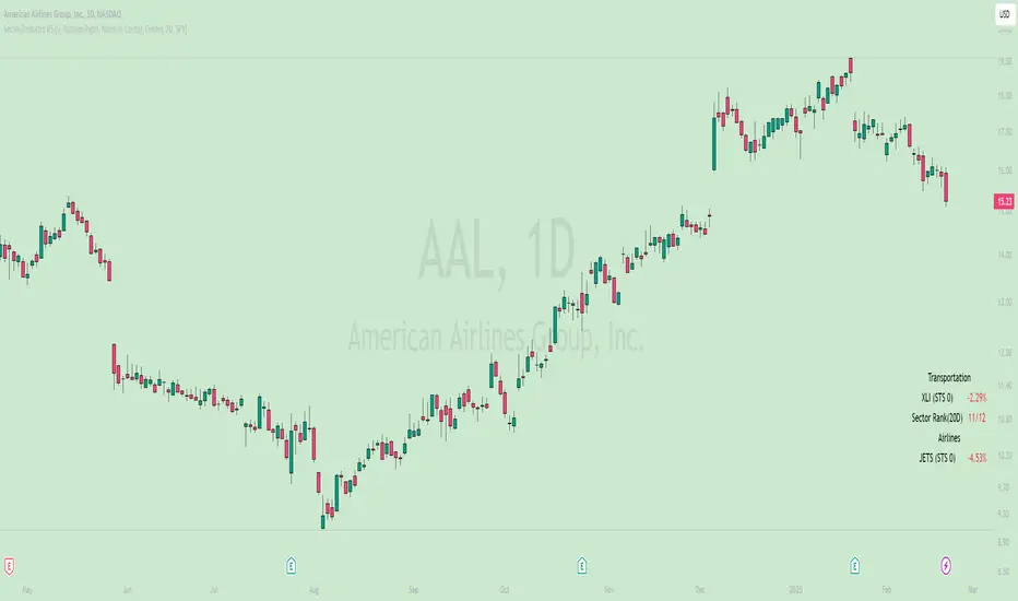
Trend & ADX by Gideon for Indian MarketsThis indicator is designed to help traders **identify strong trends** using the **Kalman Filter** and **ADX** (Average Directional Index). It provides **Buy/Sell signals** based on trend direction and ADX strength. I wanted to create something for Indian markets since there are not much available.
In a nut-shell:
✅ **Buy when the Kalman Filter turns green, and ADX is strong.
❌ **Sell when the Kalman Filter turns red, and ADX is strong.
📌 **Ignore signals if ADX is weak (below threshold).
📊 Use on 5-minute timeframes for intraday trading.
------------------------------------------------------------------------
1. Understanding the Indicator Components**
- **Green Line:** Indicates an **uptrend**.
- **Red Line:** Indicates a **downtrend**.
- The **line color change** signals a potential **trend reversal**.
**ADX Strength Filter**
- The **ADX (orange line)** measures trend strength.
- The **blue horizontal line** marks the **ADX threshold** (default: 20).
- A **Buy/Sell signal is only valid if ADX is above the threshold**, ensuring a strong trend.
**Buy & Sell Signals**
- **Buy Signal (Green Up Arrow)**
- Appears **one candle before** the Kalman line turns green.
- ADX must be **above the threshold** (default: 20).
- Suggests entering a **long position**.
- **Sell Signal (Red Down Arrow)**
- Appears **one candle before** the Kalman line turns red.
- ADX must be **above the threshold** (default: 20).
- Suggests entering a **short position**.
2. Best Settings for 5-Minute Timeframe**
For day trading on the **5-minute chart**, the following settings work best:
- **Kalman Filter Length:** `50`
- **Process Noise (Q):** `0.1`
- **Measurement Noise (R):** `0.01`
- **ADX Length:** `14`
- **ADX Threshold:** `20`
- **(Increase to 25-30 for more reliable signals in volatile markets)**
3. How to Trade with This Indicator**
**Entry Rules**
✅ **Buy Entry**
- Wait for a **green arrow (Buy Signal).
- Kalman Line must **turn green**.
- ADX must be **above the threshold** (strong trend confirmed).
- Enter a **long position** on the next candle.
❌ **Sell Entry**
- Wait for a **red arrow (Sell Signal).
- Kalman Line must **turn red**.
- ADX must be **above the threshold** (strong trend confirmed).
- Enter a **short position** on the next candle.
**Exit & Risk Management**
📌 **Stop Loss**:
- Place stop-loss **below the previous swing low** (for buys) or **above the previous swing high** (for sells).
📌 **Take Profit:
- Use a **Risk:Reward Ratio of 1:2 or 1:3.
- Exit when the **Kalman Filter color changes** (opposite trend signal).
📌 **Avoid Weak Trends**:
- **No trades when ADX is below the threshold** (low trend strength).
4. Additional Tips
- Works best on **liquid assets** like **Bank Nifty, Nifty 50, and large-cap stocks**.
- **Avoid ranging markets** with low ADX values (<20).
- Use alongside **volume analysis and support/resistance levels** for confirmation.
- Experiment with **ADX Threshold (increase for stronger signals, decrease for more trades).**
Best of Luck traders ! 🚀
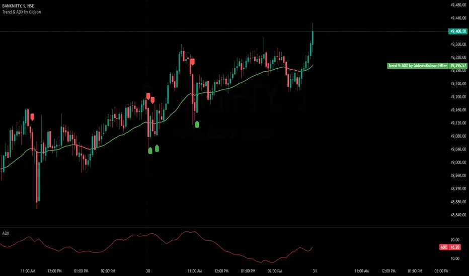
Mean Reversion Pro Strategy [tradeviZion]Mean Reversion Pro Strategy : User Guide
A mean reversion trading strategy for daily timeframe trading.
Introduction
Mean Reversion Pro Strategy is a technical trading system that operates on the daily timeframe. The strategy uses a dual Simple Moving Average (SMA) system combined with price range analysis to identify potential trading opportunities. It can be used on major indices and other markets with sufficient liquidity.
The strategy includes:
Trading System
Fast SMA for entry/exit points (5, 10, 15, 20 periods)
Slow SMA for trend reference (100, 200 periods)
Price range analysis (20% threshold)
Position management rules
Visual Elements
Gradient color indicators
Three themes (Dark/Light/Custom)
ATR-based visuals
Signal zones
Status Table
Current position information
Basic performance metrics
Strategy parameters
Optional messages
📊 Strategy Settings
Main Settings
Trading Mode
Options: Long Only, Short Only, Both
Default: Long Only
Position Size: 10% of equity
Starting Capital: $20,000
Moving Averages
Fast SMA: 5, 10, 15, or 20 periods
Slow SMA: 100 or 200 periods
Default: Fast=5, Slow=100
🎯 Entry and Exit Rules
Long Entry Conditions
All conditions must be met:
Price below Fast SMA
Price below 20% of current bar's range
Price above Slow SMA
No existing position
Short Entry Conditions
All conditions must be met:
Price above Fast SMA
Price above 80% of current bar's range
Price below Slow SMA
No existing position
Exit Rules
Long Positions
Exit when price crosses above Fast SMA
No fixed take-profit levels
No stop-loss (mean reversion approach)
Short Positions
Exit when price crosses below Fast SMA
No fixed take-profit levels
No stop-loss (mean reversion approach)
💼 Risk Management
Position Sizing
Default: 10% of equity per trade
Initial capital: $20,000
Commission: 0.01%
Slippage: 2 points
Maximum one position at a time
Risk Control
Use daily timeframe only
Avoid trading during major news events
Consider market conditions
Monitor overall exposure
📊 Performance Dashboard
The strategy includes a comprehensive status table displaying:
Strategy Parameters
Current SMA settings
Trading direction
Fast/Slow SMA ratio
Current Status
Active position (Flat/Long/Short)
Current price with color coding
Position status indicators
Performance Metrics
Net Profit (USD and %)
Win Rate with color grading
Profit Factor with thresholds
Maximum Drawdown percentage
Average Trade value
📱 Alert Settings
Entry Alerts
Long Entry (Buy Signal)
Short Entry (Sell Signal)
Exit Alerts
Long Exit (Take Profit)
Short Exit (Take Profit)
Alert Message Format
Strategy name
Signal type and direction
Current price
Fast SMA value
Slow SMA value
💡 Usage Tips
Consider starting with Long Only mode
Begin with default settings
Keep track of your trades
Review results regularly
Adjust settings as needed
Follow your trading plan
⚠️ Disclaimer
This strategy is for educational and informational purposes only. It is not financial advice. Always:
Conduct your own research
Test thoroughly before live trading
Use proper risk management
Consider your trading goals
Monitor market conditions
Never risk more than you can afford to lose
📋 Release Notes
14 January 2025
Added New Fast & Slow SMA Options:
Fibonacci-based periods: 8, 13, 21, 144, 233, 377
Additional period: 50
Complete Fast SMA options now: 5, 8, 10, 13, 15, 20, 21, 34, 50
Complete Slow SMA options now: 100, 144, 200, 233, 377
Bug Fixes:
Fixed Maximum Drawdown calculation in the performance table
Now using strategy.max_drawdown_percent for accurate DD reporting
Previous version showed incorrect DD values
Performance metrics now accurately reflect trading results
Performance Note:
Strategy tested with Fast/Slow SMA 13/377
Test conducted with 10% equity risk allocation
Daily Timeframe
For Beginners - How to Modify SMA Levels:
Find this line in the code:
fastLength = input.int(title="Fast SMA Length", defval=5, options= )
To add a new Fast SMA period: Add the number to the options list, e.g.,
To remove a Fast SMA period: Remove the number from the options list
For Slow SMA, find:
slowLength = input.int(title="Slow SMA Length", defval=100, options= )
Modify the options list the same way
⚠️ Note: Keep the periods that make sense for your trading timeframe
💡 Tip: Test any new combinations thoroughly before live trading
"Trade with Discipline, Manage Risk, Stay Consistent" - tradeviZion

Enhanced SMA Signal Box With TargetsEnhanced SMA Signal Box With Targets
The Enhanced SMA Signal Box With Targets indicator is a versatile tool designed to help traders identify buy and sell signals based on various technical analysis methods, including Simple Moving Averages (SMA), Exponential Moving Averages (EMA), and Average True Range (ATR). This indicator provides clear visual signals and target levels to assist traders in making informed decisions.
Key Features
Simple Moving Averages (SMA):
20 SMA: Represents short-term price trends.
50 SMA: Represents long-term price trends.
Exponential Moving Average (EMA):
50 EMA: Adds additional trend confirmation to the SMA.
Signal Visualization:
Buy Signals: Displayed with a green "🚀" emoji below the candle when the closing price crosses above the 20 SMA.
Sell Signals: Displayed with a red "💣" emoji above the candle when the closing price crosses below the 20 SMA.
Yellow Box: Highlights the signal candle, making it easy to identify the most recent and historical signals.
Target Prices:
First Target: Based on the size of the signal candle.
Second and Third Targets: Calculated using the ATR multiplied by a user-defined factor to help set profit-taking levels.
Customizable Filters:
MACD Filter: Users can enable this filter to use MACD line crossings for signal confirmation.
Higher Timeframe SMA Filter: Users can set a higher timeframe SMA to filter signals based on the long-term trend.
Volume Filter: Users can set a minimum volume threshold for signals.
Alerts:
Users can enable alerts for buy and sell signals, ensuring they never miss a trading opportunity.
Customizable Settings:
Line Colors and Thickness: Users can adjust the colors and thickness of the SMAs, EMA, and signal boxes.
Signal Emojis: Users can choose custom emojis for buy and sell signals.
How It Works
Trend Calculation: The indicator calculates short-term and long-term trends using the 20 SMA, 50 SMA, and 50 EMA.
Signal Generation: Buy and sell signals are generated when the price crosses the 20 SMA, with optional confirmation from MACD and volume filters.
Target Calculation: Profit targets are based on the size of the signal candle and ATR, helping traders set realistic profit-taking levels.
Important Notice
This indicator is designed for educational purposes and should not be considered as financial advice. Past performance does not guarantee future results. Users should conduct their own research and analysis before making any trading decisions. Trading involves substantial risk and is not suitable for every investor. Always consider your financial situation, investment objectives, and risk tolerance before trading. Please ensure you comply with all the relevant regulations and TradingView's house rules while using this indicator.

Logarithmic Regression AlternativeLogarithmic regression is typically used to model situations where growth or decay accelerates rapidly at first and then slows over time. Bitcoin is a good example.
𝑦 = 𝑎 + 𝑏 * ln(𝑥)
With this logarithmic regression (log reg) formula 𝑦 (price) is calculated with constants 𝑎 and 𝑏, where 𝑥 is the bar_index .
Instead of using the sum of log x/y values, together with the dot product of log x/y and the sum of the square of log x-values, to calculate a and b, I wanted to see if it was possible to calculate a and b differently.
In this script, the log reg is calculated with several different assumed a & b values, after which the log reg level is compared to each Swing. The log reg, where all swings on average are closest to the level, produces the final 𝑎 & 𝑏 values used to display the levels.
🔶 USAGE
The script shows the calculated logarithmic regression value from historical swings, provided there are enough swings, the price pattern fits the log reg model, and previous swings are close to the calculated Top/Bottom levels.
When the price approaches one of the calculated Top or Bottom levels, these levels could act as potential cycle Top or Bottom.
Since the logarithmic regression depends on swing values, each new value will change the calculation. A well-fitted model could not fit anymore in the future.
Swings are based on Weekly bars. A Top Swing, for example, with Swing setting 30, is the highest value in 60 weeks. Thirty bars at the left and right of the Swing will be lower than the Top Swing. This means that a confirmation is triggered 30 weeks after the Swing. The period will be automatically multiplied by 7 on the daily chart, where 30 becomes 210 bars.
Please note that the goal of this script is not to show swings rapidly; it is meant to show the potential next cycle's Top/Bottom levels.
🔹 Multiple Levels
The script includes the option to display 3 Top/Bottom levels, which uses different values for the swing calculations.
Top: 'high', 'maximum open/close' or 'close'
Bottom: 'low', 'minimum open/close' or 'close'
These levels can be adjusted up/down with a percentage.
Lastly, an "Average" is included for each set, which will only be visible when "AVG" is enabled, together with both Top and Bottom levels.
🔹 Notes
Users have to check the validity of swings; the above example only uses 1 Top Swing for its calculations, making the Top level unreliable.
Here, 1 of the Bottom Swings is pretty far from the bottom level, changing the swing settings can give a more reliable bottom level where all swings are close to that level.
Note the display was set at "Logarithmic", it can just as well be shown as "Regular"
In the example below, the price evolution does not fit the logarithmic regression model, where growth should accelerate rapidly at first and then slows over time.
Please note that this script can only be used on a daily timeframe or higher; using it at a lower timeframe will show a warning. Also, it doesn't work with bar-replay.
🔶 DETAILS
The code gathers data from historical swings. At the last bar, all swings are calculated with different a and b values. The a and b values which results in the smallest difference between all swings and Top/Bottom levels become the final a and b values.
The ranges of a and b are between -20.000 to +20.000, which means a and b will have the values -20.000, -19.999, -19.998, -19.997, -19.996, ... -> +20.000.
As you can imagine, the number of calculations is enormous. Therefore, the calculation is split into parts, first very roughly and then very fine.
The first calculations are done between -20 and +20 (-20, -19, -18, ...), resulting in, for example, 4.
The next set of calculations is performed only around the previous result, in this case between 3 (4-1) and 5 (4+1), resulting in, for example, 3.9. The next set goes even more in detail, for example, between 3.8 (3.9-0.1) and 4.0 (3.9 + 0.1), and so on.
1) -20 -> +20 , then loop with step 1 (result (example): 4 )
2) 4 - 1 -> 4 +1 , then loop with step 0.1 (result (example): 3.9 )
3) 3.9 - 0.1 -> 3.9 +0.1 , then loop with step 0.01 (result (example): 3.93 )
4) 3.93 - 0.01 -> 3.93 +0.01, then loop with step 0.001 (result (example): 3.928)
This ensures complicated calculations with less effort.
These calculations are done at the last bar, where the levels are displayed, which means you can see different results when a new swing is found.
Also, note that this indicator has been developed for a daily (or higher) timeframe chart.
🔶 SETTINGS
Three sets
High/Low
• color setting
• Swing Length settings for 'High' & 'Low'
• % adjustment for 'High' & 'Low'
• AVG: shows average (when both 'High' and 'Low' are enabled)
Max/Min (maximum open/close, minimum open/close)
• color setting
• Swing Length settings for 'Max' & 'Min'
• % adjustment for 'Max' & 'Min'
• AVG: shows average (when both 'Max' and 'Min' are enabled)
Close H/Close L (close Top/Bottom level)
• color setting
• Swing Length settings for 'Close H' & 'Close L'
• % adjustment for 'Close H' & 'Close L'
• AVG: shows average (when both 'Close H' and 'Close L' are enabled)
Show Dashboard, including Top/Bottom levels of the desired source and calculated a and b values.
Show Swings + Dot size

ADX and DI Trend meter and status table IndicatorThis ADX (Average Directional Index) and DI (Directional Indicator) indicator helps identify:
Trend Direction & Strength:
LONG: +DI above -DI with ADX > 20
SHORT: -DI above +DI with ADX > 20
RANGE: ADX < 20 indicates choppy/sideways market
Trading Signals:
Bullish: +DI crosses above -DI (green triangle)
Bearish: -DI crosses below +DI (red triangle)
ADX Strength Levels:
Strong: ADX ≥ 50
Moderate: ADX 30-49
Weak: ADX 20-29
No Trend: ADX < 20
Best Uses:
Trend confirmation before entering trades
Identifying ranging vs trending markets
Exit signal when trend weakens
Works well on multiple timeframes
Most effective in combination with other indicators
The table displays current trend direction and ADX strength in real-time
Arshtiq - Multi-Timeframe Trend StrategyMulti-Timeframe Setup:
The script uses two distinct timeframes: a higher (daily) timeframe for identifying the trend and a lower (hourly) timeframe for making trades. This combination allows the script to follow the larger trend while timing entries and exits with more precision on a shorter timeframe.
Moving Averages Calculation:
higher_ma: The 20-period Simple Moving Average (SMA) calculated based on the daily timeframe. This average gives a sense of the larger trend direction.
lower_ma: The 20-period SMA calculated on the hourly (current) timeframe, providing a dynamic level for detecting entry and exit points within the broader trend.
Trend Identification:
Bullish Trend: The script determines that a bullish trend is present if the current price is above the daily moving average (higher_ma).
Bearish Trend: Similarly, a bearish trend is identified when the current price is below this daily moving average.
Trade Signals:
Buy Signal: A buy signal is generated when the price on the hourly chart crosses above the hourly 20-period MA, but only if the higher (daily) timeframe trend is bullish. This ensures that buy trades align with the larger upward trend.
Sell Signal: A sell signal is generated when the price on the hourly chart crosses below the hourly 20-period MA, but only if the daily trend is bearish. This ensures that sell trades are consistent with the broader downtrend.
Plotting and Visual Cues:
Higher Timeframe MA: The daily 20-period moving average is plotted in red to help visualize the long-term trend.
Buy and Sell Signals: Buy signals appear as green labels below the price bars with the text "BUY," while sell signals appear as red labels above the bars with the text "SELL."
Background Coloring: The background changes color based on the identified trend for easier trend recognition:
Green (with transparency) when the daily trend is bullish.
Red (with transparency) when the daily trend is bearish.

Price Action All In OneThis indicator represents the most advanced level of price action indicators, incorporating six useful features: traditional gaps, shadow gaps, bar counting, moving averages, previous values, and IO pattern matching .
When I refer to price action, I mean the teachings of Dr. Al Brooks.
While you can find these features in other indicators, mine is more advanced. The default settings are designed to work on a 5-minute timeframe, but you can also use this indicator on other time periods if you prefer.
Gaps
Traditional Gaps: Occurs when the lowest price of a bar is higher than the highest price of the previous bar, or the highest price of a bar is lower than the lowest price of the previous bar.
Shadow/Tail Gaps: Occurs when the lowest price of a bar is higher than the highest price of the second last bar, or the highest price of a bar is lower than the lowest price of the second last bar.
Gaps indicate strength, and consecutive gaps in one direction are characteristic of a strong trend. They offer a perspective on the strength of a trend, signifying that limit orders on one side are at a loss with no opportunity to exit at breakeven. Can bulls or bears create gaps? Are the gaps they create filled, or do they remain open?
Traditional Gaps & Shadow/Tail Gaps
Bar Counting
The ability to use different timeframes (e.g., to determine the minute within an hour or the hour within a week).
Consistent display of 1; in other indicators, if you set intervals to 2, you see 2, 4, 6, etc., or 1, 2, 4, 6. In my indicator, you will see 1, 3, 5, etc.
In intraday trading, certain specific times are more important than others. For example, a form of reversal is more likely to occur at the midpoint of the trading day (if there are 80 candles in a day, the midpoint is at the 40th candle).
This doesn't mean you should make reversal trades at the 40th candle. The bar count feature simply reminds you of the current time, helping you gauge how long until the trading day ends. For instance, if there are 80 candles in a day and you're an intraday trader, you probably shouldn't make a swing trade at the 70th candle because there are only 10 candles left until the close—likely not enough time for a swing to develop.
Additionally, if you trade on a 5-minute timeframe, seeing candles numbered 3, 6, 9, etc. indicates the close of a 15-minute candle. This means that in addition to 5-minute timeframe traders, 15-minute timeframe traders will also pay attention to these candles, making them more significant. For the same reason, the 12th candle is crucial, as its close also marks the close of an hourly candle.
Day Time Frame & Week Time Frame
Moving Averages
Provides three EMAs. You can set different timeframes and choose between continuous or discrete modes.
Moving averages are excellent tools for determining trends. The 20 EMA is particularly popular, which increases its significance. Traders using different timeframes, such as 5-minute, 15-minute, and 1-hour, all utilize the 20 EMA. This indicator allows you to see what traders on 15-minute and 1-hour timeframes are observing, even when you're on a 5-minute timeframe.
Once again, the default settings of this indicator assume that the user is trading intraday on a 5-minute timeframe. However, if that's not the case, you can easily adjust the moving average periods. For instance, if you trade on a 1-hour timeframe and want to display the 4-hour and daily moving averages on your chart, this can be done effortlessly.
5m 20, 15m 20 & 1h 20
Previous Values
Features three previous value displays. You can set their sources and timeframes independently and define the range for all previous values.
For intraday trading, marking the previous day's high, low, and close prices can be crucial. While some other indicators provide this feature, mine does it better. You can set different timeframes and choose various sources. For example, you might want to display the average of (O+H+L+C)/4 for the last week.
In addition to setting the timeframe and source, you can also configure the display range:
All: This will show the data in all positions. For example, you can see the high price from two days ago on yesterday's chart.
Today: This will only display the previous day's high price on the current day's chart.
Timeframe: This will display the data based on the specified timeframe you set.
Last Week High, Last Day Close & Low(Timeframe Display)
IO Pattern Matching
More advanced than other IO pattern matching indicators. For adjacent IIs, it merges to display as III, IIII, and so on. The same applies to OO patterns. Additionally, it automatically merges adjacent IOI and II into IOII, and adjacent OO and IOI into IIOI.
II Pattern: This refers to two consecutive inside bar candles. On a lower timeframe, the II pattern forms a converging triangle, which is a breakout pattern. The II pattern could also potentially become a final flag, which is the last flag in a trend.
OO Pattern: This refers to two consecutive outside bar candles. On a lower timeframe, the OO pattern forms an expanding triangle. You can use the OO pattern similarly to how you would use an expanding triangle.
IOI Pattern: This pattern occurs when the first candle is contained within the second candle, and the third candle is also contained within the second candle. This is a breakout pattern and could similarly represent a terminal flag in a trend.
The appearance of II, OO, or IOI patterns does not necessarily mean you should make a reversal trade. These patterns are meant to mark potential moves in a lower timeframe within the current cycle, providing a new perspective on the market and reminding you to stay vigilant.
You shouldn't look for IO patterns in a tight trading range. There are many IO patterns in a tight trading range, but they don't hold much significance.
II, OO & IOI

Overnight Positioning w EMA - Strategy [presentTrading]I've recently started researching Market Timing strategies, and it’s proving to be quite an interesting area of study. The idea of predicting optimal times to enter and exit the market, based on historical data and various indicators, brings a dynamic edge to trading. Additionally, it is integrated with the 3commas bot for automated trade execution.
I'm still working on it. Welcome to share your point of view.
█ Introduction and How it is Different
The "Overnight Positioning with EMA " is designed to capitalize on market inefficiencies during the overnight trading period. This strategy takes a position shortly before the market closes and exits shortly after it opens the following day. What sets this strategy apart is the integration of an optional Exponential Moving Average (EMA) filter, which ensures that trades are aligned with the underlying trend. The strategy provides flexibility by allowing users to select between different global market sessions, such as the US, Asia, and Europe.
It is integrated with the 3commas bot for automated trade execution and has a built-in mechanism to avoid holding positions over the weekend by force-closing positions on Fridays before the market closes.
BTCUSD 20 mins Performance
█ Strategy, How it Works: Detailed Explanation
The core logic of this strategy is simple: enter trades before market close and exit them after market open, taking advantage of potential price movements during the overnight period. Here’s how it works in more detail:
🔶 Market Timing
The strategy determines the local market open and close times based on the selected market (US, Asia, Europe) and adjusts entry and exit points accordingly. The entry is triggered a specific number of minutes before market close, and the exit is triggered a specific number of minutes after market open.
🔶 EMA Filter
The strategy includes an optional EMA filter to help ensure that trades are taken in the direction of the prevailing trend. The EMA is calculated over a user-defined timeframe and length. The entry is only allowed if the closing price is above the EMA (for long positions), which helps to filter out trades that might go against the trend.
The EMA formula:
```
EMA(t) = +
```
Where:
- EMA(t) is the current EMA value
- Close(t) is the current closing price
- n is the length of the EMA
- EMA(t-1) is the previous period's EMA value
🔶 Entry Logic
The strategy monitors the market time in the selected timezone. Once the current time reaches the defined entry period (e.g., 20 minutes before market close), and the EMA condition is satisfied, a long position is entered.
- Entry time calculation:
```
entryTime = marketCloseTime - entryMinutesBeforeClose * 60 * 1000
```
🔶 Exit Logic
Exits are triggered based on a specified time after the market opens. The strategy checks if the current time is within the defined exit period (e.g., 20 minutes after market open) and closes any open long positions.
- Exit time calculation:
exitTime = marketOpenTime + exitMinutesAfterOpen * 60 * 1000
🔶 Force Close on Fridays
To avoid the risk of holding positions over the weekend, the strategy force-closes any open positions 5 minutes before the market close on Fridays.
- Force close logic:
isFriday = (dayofweek(currentTime, marketTimezone) == dayofweek.friday)
█ Trade Direction
This strategy is designed exclusively for long trades. It enters a long position before market close and exits the position after market open. There is no shorting involved in this strategy, and it focuses on capturing upward momentum during the overnight session.
█ Usage
This strategy is suitable for traders who want to take advantage of price movements that occur during the overnight period without holding positions for extended periods. It automates entry and exit times, ensuring that trades are placed at the appropriate times based on the market session selected by the user. The 3commas bot integration also allows for automated execution, making it ideal for traders who wish to set it and forget it. The strategy is flexible enough to work across various global markets, depending on the trader's preference.
█ Default Settings
1. entryMinutesBeforeClose (Default = 20 minutes):
This setting determines how many minutes before the market close the strategy will enter a long position. A shorter duration could mean missing out on potential movements, while a longer duration could expose the position to greater price fluctuations before the market closes.
2. exitMinutesAfterOpen (Default = 20 minutes):
This setting controls how many minutes after the market opens the position will be exited. A shorter exit time minimizes exposure to market volatility at the open, while a longer exit time could capture more of the overnight price movement.
3. emaLength (Default = 100):
The length of the EMA affects how the strategy filters trades. A shorter EMA (e.g., 50) reacts more quickly to price changes, allowing more frequent entries, while a longer EMA (e.g., 200) smooths out price action and only allows entries when there is a stronger underlying trend.
The effect of using a longer EMA (e.g., 200) would be:
```
EMA(t) = +
```
4. emaTimeframe (Default = 240):
This is the timeframe used for calculating the EMA. A higher timeframe (e.g., 360) would base entries on longer-term trends, while a shorter timeframe (e.g., 60) would respond more quickly to price movements, potentially allowing more frequent trades.
5. useEMA (Default = true):
This toggle enables or disables the EMA filter. When enabled, trades are only taken when the price is above the EMA. Disabling the EMA allows the strategy to enter trades without any trend validation, which could increase the number of trades but also increase risk.
6. Market Selection (Default = US):
This setting determines which global market's open and close times the strategy will use. The selection of the market affects the timing of entries and exits and should be chosen based on the user's preference or geographic focus.

MENTFX AVERAGES MULTI TIMEFRAMEThe MENTFX AVERAGES MULTIME TIMEFRAME indicator is designed to provide traders with the ability to visualize multiple moving averages (MAs) from higher timeframes on their current chart, regardless of the chart's timeframe. It combines the power of exponential moving averages (EMAs) to help traders identify trends, spot potential reversal points, and make more informed trading decisions.
Key Features:
Multi-Timeframe Moving Averages: This indicator plots moving averages from daily timeframes directly on your chart, helping you keep track of higher timeframe trends while trading in any timeframe.
Customizable Moving Averages: You can adjust the length and visibility of up to three EMAs (default settings are 5, 10, and 20-period EMAs) to suit your trading style.
Overlay on Price: The indicator is designed to be overlaid on your price chart, seamlessly integrating with your existing analysis.
Simple but Effective: By offering a clear visual guide to where price is trading relative to important higher timeframe levels, this indicator helps traders avoid trading against major trends.
Why It’s Unique:
Validation Timeframe Flexibility: Unlike traditional moving average indicators that only work within the same chart's timeframe, the MENTFX AVERAGES M indicator allows you to pull moving averages from higher timeframes (default: Daily) and overlay them on any chart you're currently viewing, whether it's intraday (minutes) or even weekly. This cross-timeframe visibility is critical in determining the true market trend, adding context to your trades.
Customizability: Although the default settings focus on daily EMAs (5, 10, and 20 periods), traders can modify the parameters, including the type of moving average (Simple, Weighted, etc.), making it adaptable for any strategy. Whether you want shorter-term or longer-term averages, this indicator covers your needs.
Trend Confirmation Tool: The use of multiple EMAs helps traders confirm trend direction and potential price breakouts or reversals. For example, when the shorter-term 5 EMA crosses above the 20 EMA, it can signal a potential bullish trend, while the opposite could indicate bearish pressure.
How This Indicator Helps:
Identify Key Support and Resistance Levels: Higher timeframe moving averages often act as dynamic support and resistance. This indicator helps you stay aware of those critical levels, even when trading lower timeframes.
Trend Identification: Knowing where the market is relative to the 5, 10, and 20 EMAs from a higher timeframe gives you a clearer picture of whether you're trading with or against the prevailing trend.
Improved Decision Making: By aligning your trades with the direction of higher timeframe trends, you can increase your confidence in trade entries and exits, avoiding low-probability setups.
Multi-Market Use: This indicator works well across various asset classes—stocks, forex, crypto, and commodities—making it versatile for any trader.
How to Use:
Intraday Trading: Use the daily EMAs as a guide to see if intraday price movements align with longer-term trends.
Swing Trading: Plot daily EMAs to track the strength of a larger trend, using pullbacks to the moving averages as potential entry points.
Trend Trading: Monitor crossovers between the moving averages to signal potential changes in trend direction.
Default Settings:
5 EMA (Daily) – Blue Line
10 EMA (Daily) – Black Line
20 EMA (Daily) – Red Line
These lines will plot on your chart with a subtle opacity (33%) to ensure they don’t obstruct price action, while still providing crucial visual guidance on market trends.
This indicator is perfect for traders who want to blend technical analysis with multi-timeframe insights, helping you stay in sync with broader market movements while executing trades on any timeframe.
Double BBW OverlayDouble BBW Overlay Indicator
Overview
The Double BBW (Bollinger Band Width) Overlay indicator is a custom script for TradingView that combines two BBW indicators with adjustable settings. It allows traders to compare the volatility of two different periods of Bollinger Bands on the same chart. By default, the first BBW is calculated with a 10-period center line, and the second BBW with a 20-period center line, but these values can be customized.
How It Works
Bollinger Bands consist of an upper band, a lower band, and a middle band (typically a moving average). The Bollinger Band Width (BBW) measures the distance between the upper and lower bands relative to the center line. The width of these bands indicates market volatility:
Narrow Bands: Low volatility, usually preceding a breakout.
Wide Bands: High volatility, often following a strong price movement.
This indicator plots two BBW values on a non-overlay chart, making it easy to visualize and compare different market conditions over different periods.
Indicator Components
BBW 1 (default period: 10)
Calculates the BBW using a center line based on a 10-period moving average.
The width is plotted in blue by default.
BBW 2 (default period: 20)
Calculates the BBW using a center line based on a 20-period moving average.
The width is plotted in red by default.
Zero Line
A gray horizontal line at the value of 0 for reference, helping to understand the scale of BBW values.
Input Parameters
Center Line Period for BBW 1 (length1)
Default: 10
This controls the length of the moving average for the first BBW calculation. It defines how many periods are used to calculate the middle Bollinger Band for BBW 1.
Center Line Period for BBW 2 (length2)
Default: 20
This controls the length of the moving average for the second BBW calculation. It defines how many periods are used to calculate the middle Bollinger Band for BBW 2.
Standard Deviation Multiplier (mult)
Default: 2.0
This controls how far the upper and lower Bollinger Bands are from the center line. The multiplier affects how sensitive the Bollinger Bands are to price changes, with higher values producing wider bands.
How to Use
Adding the Indicator: Once the script is added to your TradingView account, simply apply the indicator to any chart. It will be displayed as a separate pane below the price chart, showing two BBW lines corresponding to the two different periods.
Customizing Periods: Use the settings panel to adjust the center line periods for BBW 1 and BBW 2 to match your desired trading strategy. For instance, you can analyze short-term versus long-term volatility by adjusting the periods.
Volatility Analysis:
When both BBW lines are narrow, it indicates low volatility across both short-term and long-term periods, which could suggest that a breakout is imminent.
If both BBW lines widen simultaneously, it shows that volatility is increasing in both timeframes, possibly indicating a strong trend.
Use Cases
Breakout Strategy: When the BBW lines contract significantly, it may signal that a low-volatility period is about to end, which is often followed by a price breakout in either direction.
Trend Strength: Comparing short-term and long-term BBW values can help determine if recent price movements are supported by broader market volatility or if they are isolated to the short term.
Chart Display
BBW 1: Blue line, representing the Bollinger Band Width calculated with a center line period of 10 (or your customized value).
BBW 2: Red line, representing the Bollinger Band Width calculated with a center line period of 20 (or your customized value).
Zero Line: A gray line at 0 is provided for reference, although BBW values are always positive.
Advantages of Using Double BBW
Comprehensive View of Volatility: By overlaying two BBW indicators with different timeframes, you can gain insights into both short-term and long-term market volatility trends.
Customizable: You can easily adjust the moving average periods and the standard deviation multiplier to match your preferred trading strategy or the characteristics of the asset you are trading.
Easy Visualization: The separate plots of BBW values make it easier to see shifts in market volatility, allowing you to spot potential trading opportunities.
Dysmen signalsDysmen Signals Indicator
The "Dysmen Signals" indicator is designed to provide clear buy and sell signals based on the crossover of various Exponential Moving Averages (EMAs). This indicator employs a combination of short-term and long-term EMA crossovers to identify potential trading opportunities, while also highlighting significant market movements through specific signals such as the Golden Cross and Death Cross.
Indicator Components
1. Exponential Moving Averages (EMAs)
- EMA 14: A short-term EMA calculated over 14 periods.
- EMA 20: Another short-term EMA calculated over 20 periods.
- EMA 50: A mid-term EMA used as a trend filter.
- EMA 200: A long-term EMA representing the overall trend.
2. Buy and Sell Signals
- Buy Signal: This is triggered when the EMA 14 crosses above the EMA 20 and the closing price is above the EMA 50. This suggests a bullish trend in the market.
- Sell Signal: This is triggered when the EMA 14 crosses below the EMA 20 and the closing price is below the EMA 50. This indicates a bearish trend in the market.
3. Golden Cross and Death Cross
- Golden Cross (GC): Occurs when the EMA 50 crosses above the EMA 200. This is a strong bullish signal indicating a potential long-term upward trend.
- Death Cross (DC): Occurs when the EMA 50 crosses below the EMA 200. This is a strong bearish signal suggesting a potential long-term downward trend.
4. Signal Visualization
- Buy and Sell signals are marked on the chart with green and red triangles respectively. These signals help traders identify potential entry and exit points.
- Golden Cross and Death Cross signals are indicated with yellow and purple diamonds respectively, providing insight into major market trend shifts.
5. Candle Coloring
- Candles are colored green if a buy signal is active and red if a sell signal is active. This visual aid helps in quickly identifying the prevailing market sentiment.
6. EMA 200 Plotting
- The EMA 200 is plotted as a white, semi-thick line on the chart. This line serves as a reference for the overall long-term trend.
Detailed Code Explanation
- EMA Calculations: The script calculates the EMA for 14, 20, 50, and 200 periods using the ta.ema function.
- Crossover Conditions: It uses the ta.crossover and ta.crossunder functions to detect when the EMAs cross each other, triggering buy and sell signals.
- Plotting Signals: The plotshape function is utilized to display BUY and SELL signals as well as Golden Cross and Death Cross signals on the chart.
- Candle Coloring Logic: A variable direction is used to store the current market direction based on the latest signal, which then determines the candle colors using the barcolor function.
- EMA 200 Display: The plot function is used to draw the EMA 200 line on the chart with the specified color and thickness.
By employing this indicator, traders can gain valuable insights into potential market trends and make more informed trading decisions based on the crossover of key EMAs.